
Successful Pass Schedule Design in Open-Die Forging Using Double Deep Q-Learning

Institute of Metal Forming, RWTH Aachen University, 52072 Aachen, Germany
*
Author to whom correspondence should be addressed.
Processes 2021, 9(7), 1084; https://0-doi-org.brum.beds.ac.uk/10.3390/pr9071084
Submission received: 25 May 2021
/
Revised: 17 June 2021
/
Accepted: 18 June 2021
/
Published: 22 June 2021
(This article belongs to the Special Issue Modelling, Monitoring, Control and Optimization for Complex Industrial Processes)
Abstract
:In order to not only produce an open-die forged part with the desired final geometry but to also maintain economic production, precise process planning is necessary. However, due to the incremental forming of the billet, often with several hundred strokes, the process design is arbitrarily complicated and, even today, often only based on experience or simple mathematical models describing the geometry development. Hence, in this paper, fast process models were merged with a double deep Q-learning algorithm to enable a pass schedule design including multi-objective optimization. The presented implementation of a double deep Q-learning algorithm was successfully trained on an industrial-scale forging process and converged stably against high reward values. The generated pass schedules reliably produced the desired final ingot geometry, utilized the available press force well without exceeding plant limits, and, at the same time, minimized the number of passes. Finally, a forging experiment was performed at the institute of metal forming to validate the generated results. Overall, a proof of concept for the pass schedule design in open-die forging via double deep Q-learning was achieved which opens various starting points for future work.
1. Introduction
1.1. Process Design in Open-Die Forging
Open-die forging is an incremental forming process to produce predominantly longitudinally oriented components such as turbine shafts. Despite its long history, the open-die forging process has not lost any of its importance to this day. Open-die forging is characterized by the fact that not only a defined final geometry is generated, but excellent mechanical properties are also produced. Due to the incremental forming of the workpiece by commonly hundreds of strokes, the high flexibility and, at the same time, the high complexity of the process design in open-die forging arises.
In order to ensure consistent quality in industrial production, forging processes are usually designed in advance. Important process parameters, such as height reductions and bite ratios, are summed up in a so-called “pass schedule” that serves as a template for the forming process and can also be used directly to pilot the forging plant. Even today, the design of pass schedules is often based on the experience of long-standing employees or on simple mathematical models, e.g., based on volume constancy and the Tomlinson and Stringer [1] spread formulas. Although, processes designed through this approach achieve the final geometry accurately, they do not consider the expected component quality and the efficient utilization of the machine’s limits.
Pass schedule calculation programs can improve on this by including not only the geometry development but also other workpiece and process parameters, such as temperature, deformation resistance, or press force, in the pass schedule design. In this way, the generated pass schedules lead to components with the desired final geometry and, at the same time, comply with restrictions such as a maximum press force or a permissible temperature range. In addition, the consideration of higher-level objectives, such as an efficient production process by minimizing the process time, is possible. Subsequently, some typical approaches for pass schedule design in open-die forging are listed.
In 1978, Mannesmann presented the pass schedule calculation program “MD-Dataforge” [2] without publishing the underlying calculation equations. The program is able to determine the workpiece dimensions depending on the material, the temperature as well as height reduction and manipulator feed. In addition, it is checked whether the forming forces exceed the maximum press force.
Bombač et al. [3] presented the pass schedule calculation program “HFS” that uses the spread equation according to Tomlinson and Stringer (cf. Equations (1)–(3)) and a temperature calculation that is not specified in detail. The comparison of an ad hoc forging of a very experienced press operator and the pass schedule calculation program HFS shows that the pass schedules made by HFS are of at least as good quality.
Kakimoto et al. [4] integrated empirically determined results for the workpiece spread into the “Forging Guidance System (FGS)”, which allows pass schedule calculations from square to octagon and from octagon to round. After the development of an alternative spread equation and the implementation into the pass schedule calculation, the geometry model achieved an accuracy of 2% [5].
The program “ForgeBase®” [6] from SMS group GmbH resulted from the programs MD-Dataforge [2] and “ComForge” [7] and allows for the design of pass schedules under consideration of plant and material restrictions such as a permissible maximum press speed or a maximum height reduction. The user can select between different block cross-sections and forging strategies and defines the boundary conditions to be observed. In addition, pass schedules calculated with ForgeBase can be used directly to control the open-die forging plant during the process, whereby the press operator can select freely between either fully automatic, semi-automatic, or manual mode. Furthermore, previous versions of ForgeBase offered the option to optimize the generated pass schedules regarding, for example, a maximum throughput [8].
Using Tomlinson and Stringer’s expansion equation (cf. Equations (1)–(3)), Yan et al. [9] calculated pass schedules whereby the intermediate geometries for each stroke were simplified as rectangles. The simple functionality of the program implemented in MathWorks MATLAB was expanded by the informative graphical representation of individual strokes.
1.2. Machine Learning for Process Planning and Optimization in Metal Forming
Quality requirements for dimensional accuracy and material properties of forged components are continuously increasing and, therefore, the tools for process design and monitoring need to evolve accordingly. Because methods of artificial intelligence and, in particular, artificial neural networks are able to map highly non-linear interrelations well, in recent years, they have been applied progressively in the field of process design in metal forming technology. For example, Sauer et al. [10] developed deep neural networks that are able to locally predict properties such as the true strain of sheet-bulk metal parts. This locally resolved workpiece information is then integrated into the proprietary program environment SLASSY (self-learning assistance system) that supports product developers in the creation of sheet-bulk metal parts [11]. Addona et al. trained neural networks on the basis of data sets from FE simulations to generate meta models for wear-determining parameters of tools in closed-die forging [12]. These meta models then replace the computationally intensive FE simulations in a sequential optimization of the process design of the closed-die forging process.
Methods of artificial intelligence are also applied in sheet metal forming. Guo et al. as well as Dornheim et al. coupled a deep reinforcement learning algorithm to an FE simulation of a deep drawing process and trained it to regulate the blankholder force during the process. Hereby, the algorithm was trained to control the blankholder force in such a way that the finished deep-drawn part exhibited as little internal stress as possible as well as a sufficient thickness everywhere, while the manufacturing process was as material-efficient as possible [13,14,15]. Furthermore, Störkle et al. used a reinforcement learning algorithm to control the springback of the material in incremental sheet metal forming processes. The algorithm does not directly calculate the tool path but creates a modified geometry from the desired geometry that is then fed into a path planning software. The path generated in this way does not create the modified geometry but rather the desired initial geometry due to the springback [16].
Kim et al. [17] trained separate functional link neural networks (FNNs) with a single layer of neurons each to predict the resistance to forming, the spread, and the forming speed in open-die hammer forging depending on the current ingot height and width, the temperature, the height reduction, and the bite length. The training data was gathered during industrial forging processes, though no information about the individual processes and the quantity of the data was given. Furthermore, besides the results of the spread prediction using an FNN, no training results or validations were presented. Finally, an algorithm for a pass schedule calculation was described that used the FNNs to design forging processes with the greatest possible height reduction while maintaining the given force limit. This algorithm has not been validated though.
In 2018, Meyes et al. [18] described the successful use of reinforcement learning algorithms for pass schedule design in hot rolling. The database used for the training, consisting of information about the workpiece and its changes within a pass, was generated by fast process models developed at the Institute of Metal Forming (IBF). The trained algorithm can design pass schedules for rolling processes that generate a workpiece with the desired final height using as few passes as possible and, at the same time, sets a predefined grain size.
1.3. Reinforcement Learning for Pass Schedule Design in Open-Die Forging
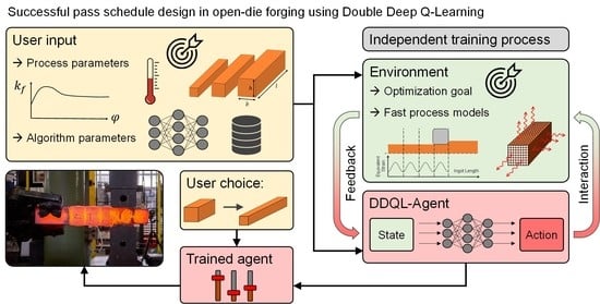
The fast process models for open-die forging presented in Section 2.1 open the possibility to predict the process and workpiece properties that result from a pass schedule quickly and, thus, to include the workpiece properties directly in the pass schedule design. In this paper, this was solved by coupling the fast models with a double deep Q-learning (DDQL) algorithm. During the training phase, the algorithm learned how to design pass schedules that, on the one hand, maintained a maximum process force and, on the other hand, led to the desired geometry as efficiently as possible. After completion of the training process, the user should be able to select any ingot geometry within the selected process window and quickly receive an optimized pass schedule. Here, the optimization goals are closely aligned to the possibilities offered by existing software for the pass schedule design mentioned above, so that comparability is ensured and, furthermore, a successfully trained DDQL algorithm can serve as a proof of concept for optimized pass schedule design in open-die forging using reinforcement learning.
For the here presented implementation of an optimized pass schedule design in open-die forging using a reinforcement learning algorithm, a rather short and simple process with approximately six passes and rectangular ingot cross-sections were selected. This enabled a broad analysis of the complex correlations between the algorithm’s behavior and its effects on the forging process, while the training durations of the required multiple training processes remain acceptable.
In future work, the presented concept will be applied on more complex forging processes featuring for example, octagonal ingot cross-sections or longer processes. Furthermore, this reinforcement learning algorithm can be extended to include, for example, the microstructure evolution into the optimization. At the same time, optimized pass schedules can be calculated very quickly so that further development of the DDQL algorithm towards a process parallel control system regarding the microstructure evolution seems possible.
2. Process, Materials, and Methods
2.1. Fast Process Modeling of Geometry, Temperature, and Equivalent Strain
The ad hoc production of any workpiece geometry with good mechanical properties requires a forging press operator to have great experience gained through a high number of trial-and-error forgings over the course of his work life. For this reason, various possibilities for process design have been established to describe the forging process in advance with regard to its main target variables: geometry, strain, and temperature. A central position is taken by finite element modeling (FEM), which, on the one hand, can calculate these parameters without restrictions for each point in the component. On the other hand, FEM requires a long calculation time, which motivates the development of faster calculation models for open-die forging. These models usually derive their high speed from the fact that compared to other calculation methods simplifying assumptions have been made which are permissible for the examined process and the examined target variables.
2.1.1. Geometry
Due to the use of geometrically simple tools and free workpiece surfaces (cf. Figure 1) the material flow in open-die forging is not predetermined but depends, among other things, on the shape and dimensions of the contact area between the ingot and the tools, the decrease in height, and on the material [19]. As shown in Figure 1, this contact area is defined by the bite length, , which corresponds to the manipulator feed, and on the ingot width, , before the forging stroke was performed. Over the course of a stroke, the initial ingot height, , is reduced to , while the initial ingot width, , increases to due to the spread. Here, the forging press applies the force, , that is required to perform the forging stroke.
To calculate intermediate and final geometries during process design and taking the free material flow in open-die forging into account, various approaches to geometry calculation based on, for example, empirical equations or the upper bound method were established.
Tomlinson and Stringer [1,21] presented simple formulae to calculate the spread and elongation of rectangular blocks, which are nowadays among the most widely used approaches mainly because of their simplicity. Forgings of steel 1.0402 (C22) were carried out by varying temperature, pressed area (initial bite width/initial width ratio ), specific height reduction , and initial width/start height ratio . Afterwards, the measured change in length can be used to determine the mean width, , of the block from Equation (1). The coefficient of expansion, s, is determined according to Equation (2). Due to the small influence of the height decrease, it can be neglected, see Equation (3).
with ; ; for 1.0402.
2.1.2. Temperature
The temperature calculation model presented by Rosenstock et al. [24] is based on the finite difference method (FDM). This approach was chosen since the 3D temperature field in open-die forging cannot be calculated with a simple analytical calculation, and it fulfills the condition of short calculation times. The FDM model considers all relevant phenomena such as convection, conduction, radiation, heat transfer to the surroundings and tools as well as dissipation during forging strokes based on the elementary theory of plasticity, see Equations (4) and (5).
where is the mean resistance to deformation of the stroke, is the yield stress, is the true plastic strain in the height direction of the stroke, is density, is specific heat, is bite length (cf. Figure 1), is height, and is the friction coefficient. The temperature increase by dissipation was modeled following the elementary theory of plasticity, where a mean value for the deformed volume of each stroke was used.
Thermal conduction in the ingot was calculated by using the implicit Crank–Nicolson method, whereas thermal radiation was implemented as an explicit boundary condition of the model with the material parameters seen in Table 2. In addition, an emissivity of = 0.85, a heat transfer to the environment of = 25 W/(m2 × K), and a heat transfer to the tools of = 4500 W/(m2 × K) were assumed.
2.1.3. Equivalent Strain
Fast models for the calculation of strain along the core fiber of a forged workpiece have been investigated on a wide range. First approaches were given by Stenzhorn [26,27] 40 years ago, which allowed for a rough estimation of the strain distribution by a linear interpolation of the values. Siemer [28] extended the model with an approximation of the evolution of the equivalent strain using a sin2 function. Following the approach of Siemer, Franzke et al. [29] adapted a model that calculated the strain of the deformed zone between the forging dies based upon the length change during forging with two empiric parameters for two-dimensional cases. Recker et al. [30] applied this model to the calculation of strain distribution after more than one forging pass.
Since these models were developed for a two-dimensional case only, Recker [20] adapted the strain model towards three-dimensional forging processes by calculating the maximum equivalent strain of a single forging stroke based on the elementary theory, see Equation (6), with as a material constant.
He also enhanced the model to only require one empiric parameter and the bite ratio , cf. Equation (7). The remaining empiric parameter, , shown in Table 3, which is the normalized length of the forming zone, was based on FEM studies and was used for the calculation of the forming zone length of one stroke .
The principle of the calculation is shown in Figure 2. For each individual stroke, a sin2 distribution of equivalent strain, which is defined by and , was imposed on the core fiber. The maximum was placed in the center of the corresponding forming zone, while the equivalent strains for the single strokes were super-imposed for the full forging sequence to obtain the distribution for the whole process or intermediate process steps.
2.2. Reinforcement Learning
Reinforcement learning is a machine learning approach based on, among others, the “trial and error” mechanism of human as well as animal learning [31]. In this learning approach, a so-called agent interacts with its environment in a goal-oriented manner and, thus, in the long term learns to maximize the positive feedback received from the environment and to avoid negative responses.
Such goal oriented and interactive learning processes also take place in the production of open-die forged components. In order to avoid the constant repetition of already known misbehavior, a plant operator strives to adapt his behavior after negative events appear, e.g., the production of scrap. In this tangible example, the plant operator represents the agent that interacts with the forging plant via the selection of process parameters (e.g., the height reduction) in order to produce a defined component as efficiently as possible as shown in Figure 3 (variant A, red). After completion of the forging process, the plant operator receives feedback about the quality of the forged product from his environment. In the industrial everyday life, this feedback could be a visual check for surface cracks or the outcome of a final quality control that classifies whether a good part or, in the worst case, scrap was produced. In this way, the plant operator builds up a broad process knowledge over the years and learns to design the forging process reasonably.
In this publication, the described learning process is realized by an independently learning agent that interacts with a virtual forging environment by selecting various process parameters in exactly the same way as a human plant operator (cf. Figure 3; variant B, green). This virtual environment represents the open-die forging process and always has a defined state that corresponds to the current ingot state (temperature, geometry, strain, etc.). The change in the ingot state, which results directly from the behavior of the agent, is calculated promptly by the fast process models described in Section 2.1 and, thus, enables an interaction between environment and agent. Through the feedback that the agent receives from the environment after each interaction, it is able to adapt its behavior in the course of a training process and, thus, to learn, e.g., how to produce desired open-die forged parts in an optimal way.
After the basic concept of reinforcement learning has been briefly outlined with the help of a practical example, the following sections first explain the most important mathematical and theoretical principles and then present the specific implementation of the generated reinforcement learning algorithm.
2.2.1. Markov Decision Processes
The concept of Markov decision processes (MDPs) offers the possibility to describe and optimize sequential decision problems and, therefore, MDPs form the basis of reinforcement learning. Markov decision processes are characterized by the fact that the probability of a future state depends only on the current state, , and the associated action, , and not on past states and actions [32]. An MDP is defined by 5 tuples that corresponds to:
- , to the set of possible states;
- , to the set of possible actions;
- to the probability of a state change from to if in state the action is chosen;
- to the scalar reward for each change of state from to ;
- , to the discount factor, which devalues any future reward and, thus, defines its value in the current time step.
2.2.2. Optimal Decision Making
During the optimization of an MDP, a selection rule, the so-called optimal policy , is sought, which assigns exactly that action, , to each state, , which maximizes the sum of the devalued rewards, the so-called return (cf. Equation (8)), in the long run [31].
In Equation (9), the Bellman equation of the action values is given, which defines a value for action choice in a state depending on the value of the action choice in the subsequent state . Here the value of an action in state corresponds to the expected return in the case that in state action is chosen and afterwards policy is followed [31].
Consequently, directly describes how good or bad an action choice in a state is with respect to the long-term generated reward in the context of the underlying decision problem. Assuming the optimal action value function is known, it follows that the optimal policy sought is to choose action in each state that maximizes [31]:
This type of policy is called greedy policy, because the decision is only made based on values of the current time step, in this case the action value function [31].
2.2.3. Q-Learning
Q-learning [33] is a widely used reinforcement learning algorithm that is able to approximate the optimal action value function by iterative fitting of a Q-function and, thus, to solve Markov decision problems [34]. The rule for the adaption of the Q-function is based on the Bellman equation (Equation (9)) for the case of an optimal action value function and the results are as follows [31]:
The Q-learning algorithm consists of an agent that interacts with an environment (cf. Figure 4) and in each discrete training time step
- receives a state information from the environment,
- then selects an action
- and finally receives a scalar reward , which describes the quality of the action choice respectively the state change made [31].
This procedure is repeated until after training steps a terminal state is reached, after which the current state is transferred back to an initial state based on defined rules. Afterwards, the training process is continued starting from the new initial state . The entirety of training time steps t, starting from an initial state to the next final state , form a training iteration.
Due to the continuous interaction between agent and environment during the training process, the algorithm independently collects experience data tuples that are used together with Equation (11) to continuously adjust the Q-function and, thus, find an approximation of the optimal action value function . Hence, a separate training data acquisition and preprocessing as needed in, for example, supervised learning algorithms is not necessary, the training data is generated during the training process.
2.2.4. Double Deep Q-Learning
Mnih et al. [35] present the deep Q-learning algorithm (DQL), which approximates the Q-function not, as usual in basic Q-learning, by a lookup table [34], but by a (deep) neural network (DNN) with the set of parameters . Thus, the algorithm is able to map finely discretized and even continuous state spaces. However, the non-linear Q-networks in combination with model-free reinforcement learning, such as Q-learning, often tend to diverge, which is why the training process can be unstable. In order to achieve good convergence properties, nonetheless, a training data memory was introduced, in which the last experience data tuples are stored. In each training step , a minibatch of randomly selected data tuples is compiled from the experience buffer and is then used to adjust the parameters of the Q-network by minimizing the loss function [36]:
The so-called target values result from the sum of the received reward and the estimated maximum Q-value of the subsequent state , which is not directly estimated by the Q-function to be learned but by an additional target Q-function [36]:
The target network corresponds exactly to the function in its structure but uses a different set of parameters . The target- parameter set is adapted to all time steps using the parameters of the current function . Overall, there are several advantages to the described procedure that increases the training stability of the DQL algorithm [35,36]:
- A higher data efficiency, since an experience data tuple is potentially trained more than once;
- Correlations between data sets of consecutive learning steps are dissolved, since the training data sets are randomly selected from the experience data memory ;
- Preventing unintentional “feedback loops”, because the current function no longer correlates directly with the current training data due to the use of the target function for the training data generation and the random compilation of minibatches.
A common problem of Q-learning algorithms is the overestimation of Q-values, which can cause a performance loss [37]. To counteract this, van Hasselt et al. [38] present the double DQL approach (DDQL), which reduces the problem of overestimation by a minor adjustment in the calculation of the target values . Within the calculation of the target values, the Q-value of the subsequent state is still determined as in DQL (cf. Equation (13)) using the target Q-function , but the best action in the subsequent state is now calculated using the maximum of the Q-function :
This decouples the selection of the best action in the subsequent time step from the estimation of the value of this selection and, thus, reduces the tendency to overestimate [37].
2.3. Implementation of the DDQL Algorithm for Pass Schedule Design in Open-Die Forging
Here, a reinforcement learning DDQL algorithm is presented that is supposed to generate optimized pass schedules following defined goals. The DDQL algorithm was chosen since deep Q- and double deep Q-learning are used successfully to solve various engineering problems [39,40,41] including the optimization of the production of multilayered optical thin films [42] whereby, as in the optimization of open-die forging processes, different highly nonlinear physical relations need to be considered. The developed algorithm was implemented in MathWorks MATLAB and consists, as described in Section 2.2 and shown in Figure 4, of two main elements interacting with each other: The agent and the environment.
The state of the environment represents the current state of the forging block and is characterized by five normalized values: The ingot height, , at the start of the current state, , the difference, , between the target height, , and the current height, , the mean equivalent strain in the core fiber, , the mean temperature in the core fiber, and the mean surface temperature, . These values were chosen based on their process information content. The current ingot height, , and the height difference, , carry needed information about the current and the target geometry and, hence, enable an estimation of the remaining process length. Since the press force is used as an optimization criterion (cf. Section 2.6), the temperature (, .) and equivalent strain () information are required, allowing a prediction of the current yield stress and consequently a prediction of forces. In addition, the mean surface temperature and the mean core temperature result in a gradient that usually increases over the course of the forging process and, consequently, allows in combination with the current ingot height, , a rough estimate of the previous process duration and the current temperature field. Based on this state information, , the agent selects the next action, , which consists of the two process parameters: bite ratio, and height reduction, . In contrast to the state information, , which consists of continuous values, the action selection of the agent is limited to discrete steps. In the present algorithm, the bite ratio, , can be varied between 0.3 and 0.9 in steps of 0.05 and the height reduction between 3% and 30% in steps of 1%.
To ensure the accuracy of the calculations from consecutive state transitions within a pass schedule, the spatially resolved information about the temperature and the equivalent strain distribution along the core fiber was stored within the environment. In subsequent passes, this information was used as the point of departure of the state transition calculations using the fast process models. Afterwards, the above-described averaged values were determined and merged together with the current geometry information in the form of the five tuple representing the resulting state .
In addition to the process parameters, such as the current ingot height or the selected height reduction , which can be directly related to the open-die forging process, the algorithm also contained parameters without a direct physical background or reference to the forging process. These included, for example, the model parameters and of the Q-networks, which were first learned during the training process using experience data tuples . Since these learned model parameters cannot be physically interpreted on their own but significantly determine the behavior of the later used algorithm and, thus, the quality of the designed pass schedules, only an indirect connection between model parameters and the forging process was present. On the other hand, the algorithm has so-called hyperparameters that are not learned during training but are predefined by the user and have no direct connection to the forging process either. Since hyperparameters significantly determine the training process of the algorithm, there is nevertheless an influence on the quality of the generated pass schedules, for example, through improved convergence properties or higher average rewards.
To approximate the Q- and target Q-values, the agent used a neural network that had two separate input branches: one for state information and one for action information. The action information was normalized and fed into the neural network by an input layer. This was followed by a fully connected layer with 24 neurons and a subsequent addition layer. This addition layer combined the pre-processed information from the two branches by an element-wise addition. In the state branch, the normalized information was also fed into the net via an input layer. Two fully connected layers followed, which were separated by a ReLu layer. The abbreviation ReLu stands for “rectified linear unit” and corresponds to the mathematical operation , where negative values are set to zero and non-negative values remain unchanged. The output of the second fully connected layer was connected to the addition layer, followed by another ReLu layer. Finally, a fully connected layer with a single neuron formed the output layer which had a value that corresponded to the estimated Q- or target Q-value. The used network architecture was proposed in [43] and shown in Figure 5.
To ensure the algorithm not only relies on its experience during the training process but also sufficiently explores the state space and action space , an ε-greedy-policy was used to maximize the return, , obtained in the long run [31]. Here, a random action, , was chosen with the probability and, otherwise with the probability of , a greedy action with respect to the value according to Equation (10) was selected. For this purpose, the agent needed to calculate the values of each combination of the current state and all possible actions separately. This was necessary because the implemented -network architecture (cf. Figure 5) uses not only the state information but also action information to determine the value of a single state–action pair. The probability ε for a random action choice does not remain constant over the training process. Starting from a value of 1, decreases continuously in every training time step according to the selected epsilon decay rate of 0.0001 to a minimum value (cf. Equation (15)). These hyperparameters are based on literature values [35] that were adapted to the conditions of the DDQL implementation in MathWorks MATLAB.
With the selected action and the present state the environment was able to calculate the change of state of the forging block using the fast process models presented in Section 2.1. A change of state does not correspond to just one pass, but always to two passes, where the forging block is rotated by 90° around the longitudinal axis after each pass. For this purpose, the bite ratio selected by the agent was used in both passes, while the selected height reduction was only used in the first pass. The height reduction in the second pass was determined in such a way that after the pass a square billet cross-section was created, taking the occurring width spread into account (see Equation (1)). This forging strategy with a square ingot cross-section after every second pass is called “square forging” and is widely used in industrial applications. Subsequently, fast process models were used to calculate the development of the temperature field and the equivalent strain distribution during both passes (see Section 2.1). Finally, the values of the state information s’ were put together and transferred to the reward function and the training data memory as shown in Figure 4.
The hyperparameters experience buffer size data sets, and the size of the mini-batch = 64 randomly chosen data sets was taken from the default settings of the DDQL implementation in MathWorks MATLAB [44]. As described in Section 2.2, the mini-batch was used to adjust the parameters and of the Q- and Target Q-networks. The learning rate determines the size of the individual adaptions and had to be lowered from the default value to based on some test trainings that showed unstable training behavior and convergence problems.
The reward function, (cf. Figure 4), is the part of the implementation in which the user defines the goals of the algorithm during the training process. For this purpose, a mathematical formulation must be found that represents the goals in such a way that the algorithm achieves them by maximizing the received return . Hence, the reward corresponds to the quality of an action choice consisting of the bite ratio and height reduction within a defined ingot state , considering the defined optimization goals.
The goals for the present application example of a pass schedule design in open-die forging were aligned to the possibilities offered by comparable pass schedule calculation software without methods of artificial intelligence (see Section 1). The first goal a pass schedule should fulfill is to reach the target geometry, whereby a permissible percentage deviation, , is tolerated. Here, this permissible deviation is one percent and is thus within the usual range for open-die forging [45]. Two further criteria for an optimal pass schedule design are derived from the desire to make the process as fast and efficient as possible. On the one hand, the final geometry should be achieved in as few passes as possible and, on the other hand, the available machine force, , should be used in the best possible way. For this purpose, the desired target force, , was set at 80% of the maximum press force, , to consider a sufficient safety margin.
Through this selection of optimization criteria with a force and a pass number component, the complicated incremental process kinematics and geometry development in open-die forgings were taken into account. If only the press force is evaluated, the algorithm could tend to apply the largest possible bite ratios while using small height reductions, resulting in long forging processes. This effect is intensified by the occurring width spread, since width spread increases with increasing bite ratios and must be forged back in the subsequent pass due to the 90° ingot rotation at the end of each pass.
On the other hand, the pure evaluation of the number of passes can lead to an algorithm selecting the largest possible height reductions combined with small bite ratios, as in this case little width spread occurs and, overall, the fewest passes are required. However, such a forging strategy can cause surface defects in the billet, such as laps, and is therefore not desirable. In addition, small bite ratios result in high numbers of strokes, which increase the process time.
Moreover, the sole evaluation of the process time is not implemented, because the process time is highly individual for each plant, as it strongly depends on the present velocities and accelerations of the manipulator and of the forging press. In addition, discrete events, such as a significant increase in time due to reheating, can hardly be weighted reasonably within the complex process optimization framework.
In Equations (16)–(18), the complete mathematical formulation of the used reward function is summarized. The function is divided into two large subareas, the evaluation of the geometry and the evaluation of the occurring maximum press force:
The reward for the generated geometry, (see Equation (17)), evaluates only the final generated ingot height of a pass schedule and not the intermediate geometry development during the forging process, as the continuous evaluation of the ingot height could cause contradictions with the other optimization goals. If the permissible final height range, , is met, the reward according to Equation (17) corresponds to a symmetrical parabola that reaches its maximum of 10 at and has the value 0 at the edges. If the algorithm generates a final height, , that falls below the minimum permissible height, , the reward corresponds to the resulting difference, . The resulting overall function for the evaluation of the block geometry, , is shown in Figure 6 (right) showing an example target height, .
Equation (17) also shows that the penalty for dropping below the final height has a lower limit of –10. This procedure is derived from the reward clipping recommended in [36] and can significantly improve the convergence properties of an algorithm, since individual rewards with high values can lead to large adjustments in the Q-function and, thus, to instability in the training process.
The evaluation of the maximum force, , occurring in the two passes of the state transition was divided into different scenarios according to its value and according to the block height, , in state (cf. Equation (18)). As long as the generated height is above the allowed end range , the reward is calculated as shown in Figure 6 (left) either by a Gaussian function or a parabola, depending on the calculated force, . If the resulting force, , corresponds exactly to the target force, , the reward reaches its maximum. If the force decreases starting from the maximum , the reward drops to −3, while for forces above , rewards up to −6 are possible. This asymmetry is due to the fact that exceeding the target force is more critical than undercutting it. If the force, , rises above the maximum press force, , reward clipping comes into effect again and limits the reward, , to a minimum of −6.
If a block height is generated that is in the range of the permitted final heights or below, the completed change of state describes the last two passes of a pass schedule. In these passes, the focus is primarily on setting the desired final geometry and not on the optimal use of the press force, which is why the force reward for forces below the target force, , is omitted (cf. Equation (18) and Figure A1 (Appendix A)). However, since the maximum press force, , must be maintained in the last two passes as well, the rest of the force evaluation () remains qualitatively unchanged.
The reward for the generated forces, , is not arbitrarily defined negatively, but it represents the goal of using the smallest possible number of passes. This results from the fact that the algorithm tries to maximize the received return, , in the course of the training and, consequently, shows a tendency to lower the number of passes, because at lower numbers of passes negative force rewards are received less often.
The total reward of an action choice is finally calculated according to Equation (16) from the sum of the geometry reward, , and the force reward, . The total reward of an action choice is also limited by reward clipping to a minimum value of −10. Therefore, the clipped sum of the individual rewards is always in the range [−10, 10] and can be scaled to the required order of [−1, 1] using the divisor 10. The general weighting of the individual parts of the reward function arose from the prioritization of the defined goals. Therefore, the reward for reaching the final geometry was set proportionally higher than the cumulative punishment of the force utilization, respectively, the number of passes. The exact weightings were determined by many test trainings.
In summary, the general characteristic of the reward function is that the focus in each of the last passes of a pass schedule is primarily on reaching the desired final height as accurately as possible and in all preceding passes, mainly on making the best possible use of the press force. To emphasize this characteristic, the discount factor was reduced from the default value = 0.99 to 0.9. Since the geometry reward is achieved only at the end of each training pass schedule, it tends to be discounted more often by the discount factor. As a result, the influence of the geometric reward granted for hitting the target height decreases in preceding passes and using the press force optimally becomes more important. However, the discount factor must not be selected too low either, since in a state , the algorithm can only select discrete actions, , and, thus, the resulting block heights, , are also limited. In addition, the permissible deviation from the target height, = , is small, and the reward received rapidly decreases with increasing distance from the optimal value , even within the permissible deviations (see Figure 6 (right)). Consequently, it may be necessary for the algorithm to adapt its actions over several passes in advance in such a way that the target height is hit as accurately as possible, thereby maximizing the total reward.
2.4. Definition of the Process Characteristics for the Pass Schedule Design in Open-Die Forging
According to [46], the weight of open-die forged parts can range from a few pounds to more than 150 tons. Furthermore, hydraulic open-die forging machines are usually offered with maximum press forces between five and two hundred meganewton [47,48,49]. Hence, the hereafter described chosen process window for the intended optimized pass schedule design using the presented DDQL algorithm with ingot weights of approximately three tons and a forging press with a maximum press force of 25 MN corresponds to a small- to medium-sized open-die forging process. Subsequently, a successfully trained DDQL algorithm can serve as a proof of concept for the pass schedule design in open-die forging via reinforcement learning.
The boundary conditions of the forging processes to be planned in an optimal manner are defined as follows:
- The assumed maximum press force, , is 25 MN. Hence, a target force of = 20 MN results;
- The initial height of the workpiece, , can be selected freely by the user between = 450 mm and = 550 mm;
- The target height of the workpiece can also be selected freely by the user between = 250 mm and = 350 mm;
- The ingot start length = 1500 mm is constant;
- The forging block consists of 42CrMo4 (1.7225), a commonly used steel for open-die forged parts. The corresponding parameters of the fast process models for temperature and equivalent strain are described in the Section 2.1.2 and Section 2.1.3, and the flow curve originates in [25];
- There is no pre-deformation of the ingot and, thus, no equivalent strain at the start of the process ( = 0);
- The ingot temperature at process start corresponds to 1000 °C and is homogeneous in the billet;
- In every second pass a bite shift of is applied. Bite shift corresponds to the offset of the contact areas between the ingot and the dies of a pass in the longitudinal direction in comparison to the contact areas of the subsequent pass;
- Since excessive cooling of the ingot during the forging process can cause damage, such as edge cracks as well as high forming forces, reheating of the forging ingot should be taken into account. This becomes necessary if the minimum temperature, , anywhere in the workpiece, including its edges and vertices, falls below a lower limit of = 650 °C.
The reheating of a hypothermic workpiece is represented by reading out the minimum block temperature, , after each change of state, respectively, for each even-numbered pass and comparing it with the minimum allowed temperature, . If the temperature falls below , the temperature field is reset to the initial state with homogeneously present temperature . Reheating is not directly considered in the reward function, since the chosen optimization criteria should lead to short processes anyway and thereby indirectly prevent mandatory reheating of the ingot.
In order to generate an algorithm that calculates pass schedules that meet the abovementioned goals while maintaining the selected process framework, the algorithm must be trained for a sufficiently long time. Therefore, the number of training iterations in the training process, which corresponds to the number of designed pass schedules, was set to 50,000 and the convergence of the algorithm was monitored (cf. Section 2.6 and Section 3.1).
At the beginning of each training iteration the state, , must be reset to the initial state, . Both the mean temperature in the core fiber, , and the mean surface temperature, , correspond in the initial state to the initial temperature, , and there is no equivalent strain, = 0. The start and target height of the forging block, and , are randomly selected within their limits for each initial state, so that the algorithm learns to generate an optimized pass schedule for all possible combinations of given input parameters.
2.5. Application of the DDQL Algorithm for Pass Schedule Design in Open-Die Forging
In Section 2.3 and Section 2.4, the implementation of the DDQL algorithm for the design of pass schedules is presented and is now completed by a description of the application of the algorithm. Therefore, Figure 7 shows the application cycle of the DDQL algorithm, which is divides into three major steps: setup, training, and usage.
At the beginning, the user (e.g., a plant operator) defines the forging process window (process parameters), while the hyperparameters of the DDQL algorithm can often remain unchanged or can be set by a programmer or a research engineer as shown in Figure 7, “Setup”. Here, together with process parameters, such as permissible geometries or material properties, the optimization goals the algorithm should pursue in the pass schedule design need to be determined, and a corresponding reward function must be formulated. The training process follows (cf. Figure 7, “Training Process”), whereby the process parameters selected by the user are incorporated into the environment and the hyperparameters into the agent as well as the framework of the training process. The environment contains not only the training goal represented by the reward function but also the fast process models (cf. Section 2.1) that calculate the change of state of the forging ingot. A training process of the implemented algorithm takes approximately two days, but once the training is successfully completed, the trained agent is able to quickly generate optimized pass schedules in the selected process window. Now, the user can select a desired initial and target geometry and receives an optimized pass schedule in a few seconds (cf. Figure 7, “Usage”).
If required, the user is able to flexibly influence all sections of the algorithm and the underlying forging process to achieve his desired pass schedule design. At the same time, the user does not need to change all sections of the algorithm at once; for example, it is also possible to change only the process parameters in an existing implementation and restart the training with the same hyperparameters and reward function to obtain an optimized pass schedule design for a different process window. However, in this case, successful training is not guaranteed, which is why the transferability of the implementation described above needs to be reviewed critically. For this purpose, the algorithm was trained on an industrial scaled forging process at first (cf. Section 3.1 and Section 3.2) and was transferred to a smaller experimental scale of the Institute of Metal Forming (IBF) for validation purposes later on (cf. Section 3.3).
2.6. Evaluation of the Algorithm Performance
To evaluate the performance and the convergence of a reinforcing learning (DDQL) algorithm, commonly the generated rewards or the Q-value of the initial state, , are plotted over the iterations of the training process [31,35,36,37,38]. If the training is successful, both values increase during the training and, in the best case, converge towards their optimum.
If an algorithm performs well measured by the generated total reward or Q-values, it is only a reliable indicator for the achievement of the defined training goals as long as the reward function is a sufficiently accurate mathematical representation of these goals. Although this condition is assumed in the present implementation, it must be checked nevertheless in the analysis of the training results. Therefore, the performance and the convergence of the algorithm are measured not only by the collected total rewards of individual iterations or the -value, but additionally by the development of the following process parameters and auxiliary variables, which directly represent the defined goals:
- Difference between the generated final height and target height ;
- ○
- Goal: accurately achieve the desired final height ;
- Number of passes ;
- ○
- Goal: minimize the number of passes;
- Maximum force occurring in the pass schedule ;
- ○
- Goal: stay below the press force limit;
- Force utilization
- ○
- Goal: best possible utilization of the forging press.
The force utilization, , corresponds to the sum of the absolute differences between the maximum generated force, , and the target force, , over all state changes that make up the evaluated pass schedule (see Equation (19)). Since the force of the last pass is not evaluated in the training process, it is also dismissed from the force utilization calculation. This procedure is based on the fact that the forces of the two passes, which are derived from the selection of an action , were not selected independently of each other due to the square forging.
Furthermore, due to the underlying non-continuous problem of pass schedule design in open-die forging, only short training iterations with mostly single-digit training step numbers occur in the present algorithm. At the same time, the structure of the reward function leads to the fact that the negative force reward is received less frequently with lower numbers of passes, which means not every combination of initial and target height can achieve the same maximum total reward. Since the start and target heights of a pass schedule are chosen randomly in the training process, the maximum possible reward is not constant within individual training iterations. For this reason, the convergence and performance of the algorithm is not measured by the characteristics of pass schedules of individual combinations of initial and target heights, but by parameters averaged over the entirety of input parameters.
To generate these mean values for different training states, the algorithm was evaluated every 2500 training iterations. The input parameters initial and target height were both varied in 20 steps, resulting in 400 evenly distributed parameter combinations. With the help of the current agent, a pass schedule was designed for each of these combinations and the abovementioned characteristic process and algorithm parameters were stored. Subsequently, an average value can be calculated for each characteristic variable across all 400 pass schedules of an evaluation step. The pass schedule design using a fully trained algorithm works in the same way as the pass schedule design during the training process, with the difference that instead of the ε greedy policy, a pure greedy policy according to Equation (10) is used.
Machine learning algorithms and especially neural networks represent black boxes which have a learning process and behavior that is very difficult or even impossible to comprehend. Therefore, the characteristics of the evaluated pass schedules are graphically refurbished to provide an insight into the behavior and the learning process of the algorithm. For this purpose, the respective characteristic parameter was plotted over the varied initial and target heights, and the individual areas were colored according to the value of the characteristic parameter. So-called heatmaps (cf. Section 3.2) arose, which enable the user to utilize his process knowledge of open-die forging to analyze the behavior of the algorithm more precisely. For example, the user can examine which training goal is already achieved for which combinations of initial and target heights or the user can analyze which process and algorithm parameters correlate.
Exactly the same algorithm might converge in one training delivering good results and diverge in another seemingly identical training producing no useful training results. This is related to random influences on the training process such as the initialization of the (target) -network and the epsilon-greedy policy. In order to ensure that the convergence of the algorithm and the generated training results are not purely by chance but resilient, the training process was carried out and analyzed 15 times with the same algorithm and process parameters but different random seeds over 50,000 training iterations each.
The training processes lasted approximately two days performed on an Intel CPU of type Xeon E-2286G. This training duration results primarily from the calculation of the environment and not from the adjustment of the network parameters. Since the DDQL algorithm has an experience data memory and consequently learns “off-policy”, the generation of experience data sets can be parallelized in the future, so that the training duration may be reduced significantly.
3. Results and Discussion
3.1. Training Outcome and Convergence
The plot of the evaluation results against the number of training iterations allows assessing the convergence of the algorithm based on the different averaged parameters. In Figure 8, this was done for all 15 trainings in form of box plots.
Figure 8a shows the average total reward, , obtained by a pass schedule. The algorithm converges robustly against the same averaged reward in all 15 trainings. However, it was noticeable that there were single outliers, which are represented by red crosses. These can be traced back to the learning steps of the agent that were taken shortly before the evaluation in which the designed processes have changed significantly. Due to the changed behavior, the algorithm often reaches areas of the state space, , in which it does not have a good approximation of the optimal action value function yet and, therefore, performs poorly. The fact that these outliers were not transferred to the following evaluation steps shows that the algorithm quickly learns to select the right actions even in the new states and, consequently, achieves higher rewards again.
It follows that the agent of the last training iteration was not necessarily the best one. The best agent was the one that has the highest averaged reward compared to all the other evaluations of the training process [38] while always hitting the final height range and respect the maximum press force, . Hence, hereafter, the best agent determined in this way represents the training outcome. The number of training iterations of the best agents ranged between 22,500 and 50,000 iterations and amounted to an average of ~37,500 iterations. In addition to the development of a variable, the box plot of the 15 best agents of all trainings is shown on the right-hand side of each single graphic of Figure 8. The best averaged rewards were very close together except for one value, which receives a slightly lower maximum reward. This accentuates the good convergence of the algorithm.
In Figure A2, the plot of the averaged Q-values of the initial states against the number of training iterations is shown. The graph has qualitatively the same course as the graph of the generated rewards. Since the Q-function does not approximate the summed reward , but the received return, , it ran below the total reward. This also emphasizes the stability of the training process and the good convergence properties of the presented algorithm.
After the general convergence of the algorithm has been demonstrated, it must be checked whether the defined goals for the optimized pass schedule design in open-die forging were achieved over the course of the trainings. Therefore, the development of the force utilization, , the deviation from the target height, , and the number of passes, , throughout all 15 trainings is shown in Figure 8 as well. Figure 8b shows that the force utilization drops to a value of approximately one meganewton during the first 20,000 iterations of the training process and remains constant in this range from then on. The 15 best agents achieved an average force utilization of less than one meganewton. Considering a target force of = 20 MN, this corresponded to a deviation of less than 5%, showing that the goal of optimal press force utilization was reached.
The mean deviation from the target height, , converged significantly faster compared to the mean force utilization, , and already shows deviations of less than 0.4% on average during the first evaluation after 2500 training iterations and, thus, clearly undercuts the targeted maximum permissible deviation of 1% (see Figure 8c). Due to the very early achievement of this goal, the graph does not show the typical convergence curve, but is constant at low values around 0% 0.5% deviation. However, a slight bias towards positive deviations, , or towards exceeding the final height, , was evident. This bias could result from the nature of the training process, since the reward for setting the final height was symmetrical on both sides. If the algorithm exceeds the allowable final height, it only has to accept the negative force reward of an additional pass but can still receive the big positive reward for setting the final height with another pass. This is not possible if the final height is undershot, so the algorithm probably tends to exceed the target height. The box plot of the 15 best agents was very close to a 0% deviation and showed the described bias only very slightly, which confirms the set geometry target had been met.
Figure 8d shows the development of the average number of passes in the 15 training processes carried out. The mean number of passes, , decreased in the course of the training and finally converged after approximately 25,000 iterations in a range of approximately 5.6 passes confirming the achievement of the last goal, the minimization of the number of passes, .
However, it is noticeable that the algorithms did not converge against one, but against several similarly small average numbers of passes = ~6.1, = ~5.6 and = ~5.2. These different numbers of passes do not result in total rewards that differ to the same extend (see Figure 8a), since e.g., a higher reward from lower numbers of passes can be equaled out by lower force and geometry rewards. Consequently, there is probably no clearly defined global maximum in the current reward function.
A comparison of the convergence times of the individual process variables reveals that first the geometry target (approx. 0–2500 iterations), then the force target and finally the target of the lowest possible number of passes is attained. This sequence corresponds to the weightings that the individual reward components take up within the total reward and occurs in all 15 training sessions.
Overall, the analysis of the 15 training processes revealed that the agent trained robustly and converged reliably towards high rewards. At the same time, the development of the characteristic process variables corresponded to the formulated goals for the pass schedule design in open-die forging, which proves the suitability of the reward function.
3.2. Best Agent Results
After Section 3.1 presented the convergence properties of the algorithm and the development of the characteristic parameters in the course of the training, this chapter constitutes the overall best training result throughout all 15 accomplished trainings in more detail. This result arose in the 45,000th iteration of the fifteenth training process and achieved an average total reward of = 0.76 in the evaluation.
As shown in Figure 9a, the deviations from the target height, , were below the limit of in each of the 400 pass schedules, with the maximum deviation being -0.66%. On average, the agent reached a deviation of = 0.22%. The force utilization shown in Figure 9b averaged at = 0.75 MN and was, at most, just over two meganewtons. As seen in Figure A3b, the maximum force of 25 MN was not exceeded in any pass schedule but always undercut by at least 3 MN. Figure 9c shows the number of passes, , via the input parameter space. There were three clearly separated areas of different numbers of passes, starting from four passes at small initial heights and large target heights, over six passes to eight passes at large initial heights and small target heights. The mean number of passes, , was 5.20. Since more passes cause a negative force reward more often and the algorithm was able to approximate this correctly, the heat map of the Q-values in the initial state, , shows the same three distinct ranges as the heat map of the number of passes (see Figure A3a).
On closer examination of the heat maps for the deviation from the target height, , and the force utilization, , patterns were noticeable. In the heatmap of the force utilization (cf. Figure 9b), these slight patterns ran predominantly parallel to the ordinate and were best seen in the four-pass area on the top left. Here, it can be observed that the force utilization, from left to right, repeatedly increased at first and then abruptly dropped. In the four-pass area (top left) of the heatmap of the target height deviation (cf. Figure 9a), a diagonal pattern was present that consisted of a fixed sequence of slightly undershooting the target final height, a good agreement with the final target height and slightly overshooting the target final height. This diagonal pattern changed its orientation in the six and eight pass regions (central and bottom right), although it was not as distinct in the eight as in the six-pass area of the heatmap.
The described patterns were partially caused by direct correlations between different process parameters. For example, at pass number transitions, the press force tended to be used less efficiently and the target height was hit the worst. On the other hand, such patterns can result from the restriction of the discrete action selection. Due to the discrete action selection, , the set of possible geometries in the subsequent state, , was also discrete and dependsed directly on the geometry of the current state, , and the discretization of the actions, .
Starting from an ingot geometry in state, , the algorithm could only realize a discrete quantity of geometries in state due to the limited discrete number of actions, . Including another action choice in state from the discrete set of actions, , the quantity of possible discrete geometries, , increases exponentially, because now the intermediate geometry in state can be adjusted specifically. Consequently, the quantity of possible discrete geometries in a final state of a pass schedule design increases exponentially with the number of action choices (i.e., passes) the algorithm can take into account before reaching the final geometry. With only four passes to reach the final geometry, however, the number of possible actions and realizable discrete geometries, , is significantly limited.
In addition, the reward, , obtained decreases rapidly over the narrow allowed final height range, so that the algorithm is usually not able to obtain the maximum geometry reward only by the action choice of the last pass. In order to be as close as possible to the target geometry and, thus, maximize its reward, the algorithm must also adjust the parameters of the previous passes in such a way that the last intermediate geometry in combination with the allowed discrete action choices can the target height be achieved as accurately as possible. While adjusting the parameters of previous passes, the algorithm accepts reduced force rewards in order to achieve higher geometry rewards, whereby the vertical patterns in the heat map of the force utilization arise (cf. Figure 9b). However, the algorithm cannot always perfectly hit the target height, even when taking previous passes into account, which results in fine patterns in the heatmap of the deviation from the final height. These patterns are significantly more distinct in the four-pass area than in the areas with six or eight passes, since the quantity of possible geometries, , is significantly more limited in this area as described above.
Due to the connection in the form of the reward function, , the described patterns can also be found in an attenuated form and partly overlaid in the heatmap of the collected total reward, . For example, the average reward in the four -pass area was higher than in the six- and eight-pass areas due to the negative force rewards and, also, the patterns from the deviations from the target height as well as the patterns observed in the force utilization were recognizable.
Behavior Analysis Using an Example Pass Schedule
In the two previous chapters, the results of the generated pass schedules were analyzed and evaluated on the basis of different partially averaged parameters. Therefore, in this chapter, a tangible example pass schedule is used to show how the algorithm was choosing the actions consisting of a bite ratio and height reduction in order to generate the optimized pass schedules.
The billet had an initial height and width of of 512.5 mm, which was reduced to a target height and width of = = 267.5 mm over the course of the forging process. The remaining process boundary conditions corresponded to those listed in Section 2.4. Since the implemented pass schedule design was based on the square forging strategy, the forging block was rotated by 90° around the longitudinal axis after each pass. The pass schedule (see Table 4) was generated using the action choices of the best agent (training process 15, iteration 45,000), and it contained all the necessary variables, such as ingot dimensions and process and plant characteristics, which are required to carry out the forging process.
In addition to the maximum force, a mean force was listed to provide the machine operator with a better estimation of the expected forces during the forging process. This was calculated from the individual forces of all strokes except those at the ends of the workpiece, since smaller bite widths can occur in these due to the bite shift or smaller final strokes.
An examination of the selected height reductions and bite ratios, which are representative for the training sessions performed, shows that the algorithm tended to select the largest possible height reductions, , in all but the last passes combined with rather small bite ratios, . Only if the target force is not reached by this strategy, it increases the bite ratio until the desired force is attained. Since the final height is defined in the last two passes and the force must not exceed the force limit, the action selection of the algorithm directly results from this. Bite ratio and height reduction are chosen in a way that the final height is hit as exactly as possible, taking the occurring spread into account and, consequently, maximizing the received reward, . As already described in Section 3.2, due to the discrete action choices, it may be necessary to deviate slightly from the described selection behavior at certain times in order to obtain the maximum geometry and force reward.
Utilizing this procedure, the algorithm hits the desired final geometry, represented by the target height (=target width), excellently and uses the available press force well at the same time. In addition, the tendency towards small bite ratios results in a tendency towards less spread and, thus, a lower number of passes. Furthermore, as soon as the bite ratio is increased to generate the desired target force, the number of strokes per pass decreases, which leads to a reduction in the total process time. Overall, this procedure for the pass schedule design of the algorithm is adequate and reasonable in the context of the selected optimization goals. Nevertheless, in the shown example, the parameter selection of the last pass may be different in an experience-based pass schedule, since the algorithm selected a small bite ratio of 0.3 and, hence, did not utilize the forging press to its capacity. This choice resulted from the fact that in the last pass, the reward of the generated force was omitted and only the deviation from the final height was evaluated. In combination with the discrete action selection, the chosen combination of bite ratio and height reduction presumably maximized the received reward in the last pass. In industrial processes, a larger bite ratio may be more appropriate, because the press force is not yet exhausted, and a higher bite ratio would reduce the process time even further due to the decreasing stroke numbers in the last pass. In this case, the height reduction would also have to increase, as a larger bite ratio is associated with more width spread. Such an increase of bite ratio and height reduction is only possible and useful as long as the increased width spread does not cause higher number of passes.
3.3. Experimental Validation
In order to validate the applicability of the generated optimized pass schedule design via an DDQL algorithm, a forging experiment was carried out on the forging plant of the Institute of Metal Forming of the RWTH Aachen University (IBF). The setup consisted of a 6.3 MN forging press and a 6 axis heavy-duty robot. Since the pass schedule design presented so far was based on an industrial-scale forging process, first, the process parameters in the algorithm implementation were adapted to the conditions at the IBF and, afterwards, the adjusted algorithm was trained again. Therefore, a quadratic ingot cross-section of 150 mm × 150 mm (height × width) was chosen, since these are the biggest ingot dimensions that can be reliably gripped and manipulated. Hence, to ensure a reasonable process design and to match the ingot dimensions the maximum press force, , was reduced from 25 MN to 3.5 MN, resulting in a target force, = 2.8 MN. The permissible initial and target heights of the forging block were set to = 135–165 mm and = 75–105 mm. The initial block length, , corresponded to 500 mm. In addition, the press speed was halved to 50 mm/s and the maximum height reduction was reduced from 30% to 25%. The forging ingot was made of a low-cost low alloyed steel of grade C45. The material-dependent parameters for the temperature and spread calculation as well as the yield stress were changed accordingly [1,25]. Furthermore, the process time calculation was adjusted to the real process conditions at the IBF, e.g., by adding a transport time from the oven to the press of 45 s as well as break times of 15 s between individual passes. This is necessary because full automation was assumed in the so far considered industrial process window, which was not achieved at the IBF forging plant to this degree. All other process and algorithm parameters remain unchanged (cf. Section 2.3 and Section 2.4) and the adapted DDQL algorithm was trained only once.
Even with the new significantly different process window, the algorithm successfully converged after 50,000 training iterations against an average reward of = ~0.63. Due to the changed geometry spectrum, the generated pass schedules contained more passes, which is why the overall reward was lower compared to the industrial process. The best agent occurred after 35,000 training iterations and produced a mean number of passes of = 6.56, a mean force utilization of = 0.2 MN, and a mean deviation from the target end height of = 0.22%. Consequently, the formulated optimization goals for the pass schedule design were also achieved for this modified process window. The associated heat maps of the characteristic process and algorithm parameters of the best agent are appended to this publication (see Figure A4).
The pass schedule used in the experiment was generated in advance using the best agent of the successfully trained adapted DDQL algorithm and is listed in Table 5.
In the forging experiment at the IBF (cf. Figure 10), the positioning of the ingot before the first stroke of each pass was done manually. Consequently, the bite length and the press force of the strokes at the ingot ends could fluctuate. For this reason, the maximum press force of each pass, which occurred at one of the block’s ends due to the stronger cooling, could not be used as a reliable benchmark. Instead of this, the averaged forces of the middle strokes, which were not affected by bite length fluctuation due to the manual handling, were compared. Hence, the compared mean forces (see Figure 11) were lower than the maximum predicted forces within a pass (cf. Table 5).
During the experiment, the process time and the occurring press forces were measured and, subsequently, the abovementioned averaged measured force, , as well as the averaged predicted force, , were evaluated for every pass (see Figure 11). In addition, Table 6 gives an overview of the strokes taken into account and the standard deviations that occurred for each pass.
Figure 11 shows that the created DDQL algorithm was able to predict the real press forces both qualitatively and quantitatively. The mean measured forces, , deviated from the mean predicted forces, , by an average of 9.7% and a maximum of 19.9%, which emphasizes the estimated target force of for the algorithm. Over the process, the measured force increased continuously compared to the predicted force, , and exceeded it from the fifth pass. The continuous increase could have resulted from the delay between the timeline of the experiment and the timeline of the designed pass schedule that increased from −13.6 s at the end of pass one to 93 s at the end of pass six (cf. Table 6 and Figure 11). This delay appeared despite the abovementioned adapted time calculation, since the break time in between different passes, needed for manual handling of the forging ingot, was slightly underestimated. The longer process duration can cause a stronger cooling of the forging ingot compared to the prediction of the algorithm, thus, to higher yield stresses and ultimately to higher press forces.
Moreover, deviating flow curves, model inaccuracies of the force and temperature calculation as well as real process conditions, such as fluctuating initial ingot temperatures or slight deviations in the chemical composition of the material, can lead to deviating press forces.
In combination with the results of the optimized pass schedule generation already presented (cf. Section 3.1 and Section 3.2), the findings of the forging experiment accentuate the capability of the generated DDQL algorithm to produce optimized pass schedules for real open-die forging processes. Here, the press forces were predicted with sufficient accuracy and the generated pass schedules efficiently used the available press force. In addition, the final height was reliably reached, and the number of passes was reduced to a minimum within the given conditions.
4. Conclusions and Outlook
In this paper, a DDQL algorithm was presented that learned to design optimized pass schedules autonomously with the help of fast process models. The training process was stable and independent of the selected process window (industrial-scale forging/test forging at institute), the selected material (42CrMo4/C45), and the random seed. Moreover, the algorithm converged reliably in all training scenarios. This shows that the selected algorithm and its hyperparameters are well suited for the introduced problem of pass schedule design in open-die forging and, at the same time, emphasizes the transferability of the presented approach. The algorithm can be flexibly transmitted to other square forging processes by changing the process boundary conditions as well as the geometry, while the retraining does not require an adjustment of the hyperparameters. After the training process that takes about two days, the algorithm was able to design optimized pass schedules in two to four seconds, which makes the concept of pass schedule design in open-die forging using a DDQL algorithm altogether well suited for industrial use.
The pass schedules generated by the trained algorithms fulfilled the formulated goals. They created the desired final geometry while maintaining the permissible target height deviation of one percent. At the same time, with an average deviation of less than 5%, a very good utilization of the available press force was realized (cf. Section 3). In addition, the maximum press force was never surpassed in all 6000 pass schedules of the 15 training outcomes, and the average number of passes was reduced to a minimum = 5.6 within the given conditions. This also shows the developed reward function was a good mathematical formulation of the defined optimization goals, since all set goals could be achieved in the course of the trainings.
During the development of the DDQL algorithm, the important role of the reward function became clear, because the reward function first had to be extended by reward clipping (see Section 2.3) and the weightings of the individual reward parts had to be varied before a stable training process with useful results could be achieved. Consequently, the reward function not only determines the quality of the generated pass schedules but also contributes significantly to the success of the training process. In addition, the average number of passes, , over the training process (see Figure 8d) showed a slight scatter in the convergence limits. This could be an indication that the global maximum of the reward function was not clearly defined and an improvement in this could lead to even better convergence properties. Overall, the development of a good reward function is a crucial factor in the application of reinforcement learning, which is why a more detailed investigation and optimization of the reward function is desirable.
Despite the good results and the finely discretized evaluation with 400 sampled schedules each, the utilized neural networks represent black boxes which display behavior that cannot be predicted for each individual case. For this reason, a pass schedule designed via machine learning should not go unchecked before it is used in the production process. To assure this, for example, the calculated maximum press force and the final geometry can be output, and the observance of the strict limits can be checked beforehand either automatically or by a forging press operator.
Furthermore, the usage of heat maps to visualize evaluation results can help to gain deeper insights into the normally opaque training process of neural networks. The training results of an input parameter space can be clearly displayed and, thus, interpreted by the user. This facilitates, for example, the creation of practicable reward functions, because it is possible to comprehend which process parameters are changed in what way and at what time during the training. In addition, the use of heat maps also enables the user to find correlations between different process and algorithm parameters, such as the influence of the discrete action selection on the target height deviation and the force utilization, which caused patterns in the corresponding heat maps (cf. Section 3.2).
Due to the reliable convergence of the algorithm and the good achievements of the optimization goals, it can be concluded that the presented DDQL algorithm offers the same possibilities for optimized pass schedule design as conventional pass schedule calculation tools (see Section 1). Therefore, the presented algorithm serves as proof of concept for the optimized pass schedule design in open-die forging via double deep Q-learning and, furthermore, as a starting point for further work.
Since the presented implementation of the DDQL algorithm was based on rather simple forging processes an extension to longer or more complex forging processes with different ingot cross-sections, for example, octagonal seems useful. The required fast process models for octagonal cross-sections are available [23].
Furthermore, the presented algorithm used neural networks that can map highly non-linear relationships; hence, the chosen approach is ideally suited to include other important process and material parameters in the pass schedule design. In the future, the environment could be extended by an already existing semi-empirical fast model for microstructure calculation [50], so that, for example, the generation of a defined grain size may be included in the goals for the optimized pass schedule generation. In addition, an extension of the action selection of the agent by a variable bite shift is conceivable; hence, the agent has the possibility to create homogeneous equivalent strain distributions. With such additions, the functional range of the DDQL algorithm would exceed that of the conventional pass schedule calculation approaches and could therefore contribute to continuous quality improvement of open-die forgings.
The successful offline design of optimized pass schedules using a DDQL algorithm also opens up the opportunity for an online process optimization, since an online process control can be understood as a process design starting from an intermediate process state. Furthermore, the calculation times of the pass schedule design are sufficiently short, and the neural networks used in the reinforcement learning algorithm may be able to depict the more complex correlation in an online process control. Hence, in combination with an existing microstructure model [50] even the online control of the microstructure seems possible.
Author Contributions
Investigation, N.R.; Conceptualization; N.R., F.R., S.G., D.B., and G.H.; writing—original draft preparation, N.R. and F.R.; writing—review and editing, N.R., F.R.; S.G., D.B., and G.H.; supervision, S.G., D.B., and G.H. All authors have read and agreed to the published version of the manuscript.
Funding
This work was funded by the Deutsche Forschungsgemeinschaft (DFG, German Research Foundation)—452539735.
Data Availability Statement
The program code of the fast process models (Section 2.1) and of the described DDQL algorithm (Section 2.3) is not publicly available.
Conflicts of Interest
The authors declare no conflict of interest.
Appendix A
Figure A1.
Plot of the Force reward, , over the ratio of the produced force, , and the maximum allowed Force, , in case the current height, , is equal or lower than the maximum final height , and thus the related state, , is a terminal state, .
Figure A1.
Plot of the Force reward, , over the ratio of the produced force, , and the maximum allowed Force, , in case the current height, , is equal or lower than the maximum final height , and thus the related state, , is a terminal state, .

Figure A2.
Boxplots of the mean Q-value of the initial state, , of all 15 trainings over the course of the training process.
Figure A2.
Boxplots of the mean Q-value of the initial state, , of all 15 trainings over the course of the training process.

Figure A3.
Heatmaps of the training results of the overall best agent (training 15, iteration 45,000): (a) initial Q-value and (b) the maximum occurred force in a single pass schedule, .
Figure A3.
Heatmaps of the training results of the overall best agent (training 15, iteration 45,000): (a) initial Q-value and (b) the maximum occurred force in a single pass schedule, .

Figure A4.
Heatmaps of the training results (best agent) of the forging experiment: (a) the target height deviation, , (b) the mean force utilization, , (c) the mean number of passes, , (d) the total reward , (e) initial Q-value and (f) the maximum occurred force in a single pass schedule, .
Figure A4.
Heatmaps of the training results (best agent) of the forging experiment: (a) the target height deviation, , (b) the mean force utilization, , (c) the mean number of passes, , (d) the total reward , (e) initial Q-value and (f) the maximum occurred force in a single pass schedule, .

References
- Tomlinson, A.; Stringer, J.D. Spread and elongation in flat tool forging. J. Iron Steel Inst. 1959, 193, 157–162. [Google Scholar]
- Mannesmann Demag Hüttentechnik. MD-Dataforge—The Program Control System for MD-Open Die Forge Plants; Mannesmann Demag Hüttentechnik: Mönchengladbach, Germany, 1990. [Google Scholar]
- Bombač, D.; Fazarinc, M.; Kugler, G.; Turk, R. Tool for programmed open-die forging–case study. RMZ-Mater. Geoenviron. 2008, 55, 19–29. [Google Scholar]
- Kakimoto, H.; Choda, T.; Takamori, H.; Takahashi, Y.; Takahara, H.; Takahashi, I. Renewal of Oil Hydraulic Press and Optimization of Forging Pass Design to Improve Productivity. In Proceedings of the 16th Internationl Forgemasters Meeting, Sheffield, UK, 15–19 October 2006; pp. 231–240. [Google Scholar]
- Kakimoto, H.; Takashi, Y.; Takamori, H.; Tanaka, T.; Imaida, Y. Process Design of Extend Forging Process Using Numerical Simulation Development of Process Design Method for the Finish Forging Process. Mater. Trans. 2009, 50, 1998–2004. [Google Scholar] [CrossRef]
- SMS Group GmbH. Open-Die Forging Plants: Tailormade Solutions; SMS Group GmbH: Mönchengladbach, Germany, 2021; Available online: https://www.sms-group.com/press-media/media/downloads/download-detail/download/17560 (accessed on 26 February 2021).
- Nieschwitz, P.; Ecken, F.-P.; Siemer, E. COMFORGE Program for pass-schedule calculation in open-die forging. In Verein Deutscher Eisenhüttenleute VDEh; Stahl und Eisen, No. 12; Association of Steel and Ironworks: Düsseldorf, Germany, 1988; pp. 55–60. [Google Scholar]
- Schmitz, W. ForgeBase—A Tool for Optimization of the Open-Die Forging Process. In Proceedings of the 15th International Forgemasters Meeting, Kobe, Japan, 26–29 October 2003. [Google Scholar]
- Yan, C.; Gao, F. Simulation of programmed incremental open-die forging processes based on spread coefficient and geometric transformation. Proc. Inst. Mech. Eng. Part E J. Process Mech. Eng. 2010, 224, 129–135. [Google Scholar] [CrossRef]
- Sauer, C.; Küstner, C.; Schleich, B.; Wartzack, S. Einsatz von Deep Learning zur ortsaufgelösten Beschreibung von Bauteileigenschaften. Des. X-Beiträge Zum 2017, 28, 49–60. [Google Scholar]
- Sauer, C.; Schleich, B.; Wartzack, S. Deep learning in sheet-bulk metal forming part design. In Proceedings of the DESIGN 2018 15th International Design Conference, Dubrovnik, Croatia, 21–24 May 2018; Faculty of Mechanical Engineering and Naval Architecture, University of Zagreb: Zagreb, Croatia; The Design Society: Glasgow, UK, 2018; pp. 2999–3010. [Google Scholar]
- D’Addona, D.M.; Antonelli, D. Neural Network Multiobjective Optimization of Hot Forging. Procedia CIRP 2018, 67, 498–503. [Google Scholar] [CrossRef]
- Guo, P.; Yu, J. Optimal Control of Blank Holder Force Based on Deep Reinforcement Learning. In Proceedings of the 2019 IEEE International Conference on Industrial Engineering and Engineering Management (IEEM), Macao, China, 15–18 December 2019; IEEE: Piscataway, NJ, USA, 2019; pp. 1466–1470, ISBN 978-1-7281-3804-6. [Google Scholar]
- Dornheim, J.; Link, N. Multiobjective Reinforcement Learning for Reconfigurable Adaptive Optimal Control of Manufacturing Processes. In Proceedings of the 2018 International Symposium on Electronics and Telecommunications (ISETC), Timisoara, Romania, 8–9 November 2018; Available online: https://arxiv.org/pdf/1809.06750 (accessed on 17 June 2021).
- Dornheim, J.; Link, N.; Gumbsch, P. Model-Free Adaptive Optimal Control of Episodic Fixed-Horizon Manufacturing Processes using Reinforcement Learning. Int. J. Control Autom. Syst. 2019, 18, 1593–1604. [Google Scholar] [CrossRef] [Green Version]
- Stoerkle, D.D.; Seim, P.; Thyssen, L.; Kuhlenkoetter, B. Machine Learning In Incremental Sheet Forming. In Proceedings of the ISR 2016: 47st International Symposium on Robotics, Munich, Germany, 21–22 June 2016; VDE: Berlin, Germany; IEEE: Piscataway, NJ, USA, 2016. [Google Scholar]
- Kim, P.H.; Chun, M.S.; Yi, J.J.; Moon, Y.H. Pass schedule algorithms for hot open die forging. J. Mater. Process. Technol. 2002, 130-131, 516–523. [Google Scholar] [CrossRef]
- Meyes, R.; Tercan, H.; Thiele, T.; Krämer, A.; Heinisch, J.; Liebenberg, M.; Hirt, G.; Hopmann, C.; Lakemeyer, G.; Meisen, T.; et al. Interdisciplinary Data Driven Production Process Analysis for the Internet of Production. Procedia Manuf. 2018, 26, 1065–1076. [Google Scholar] [CrossRef]
- Pahnke, H.J. Grundlagen des programmierten Schmiedens. In Verein Deutscher Eisenhüttenleute VDEh; Stahl und Eisen; Association of Steel and Ironworks: Düsseldorf, Germany, 1983; Volume 103, pp. 547–552. [Google Scholar]
- Recker, D. Entwicklung von Schnellen Prozessmodellen und Optimierungsmöglichkeiten für das Freiformschmieden; Shaker: Aachen, Germany, 2014; ISBN 9783844028478. [Google Scholar]
- Tomlinson, A.; Stringer, J.D. The Closing of Internal Cavities in Forgings by Upsetting. J. Iron Steel Inst. 1958, 196, 209–217. [Google Scholar]
- Nieschwitz, P. Wege zur Qualitätssteigerung beim Freiformschmieden; Stahleisen: Düsseldorf, Germany, 1988; ISBN 9783514004092. [Google Scholar]
- Rosenstock, D. Schnelle Prozessmodellierung, Online-Visualisierung und Optimierung beim Freiformschmieden; Verlagshaus Mainz GmbH: Aachen, Germany, 2017; ISBN 9783958862043. [Google Scholar]
- Rosenstock, D.; Recker, D.; Hirt, G. Online Analysis of Cogging Processes–Evaluation of the Equivalent Strain, Temperature and Grain Size Distribution. In Proceedings of the 19th International Forgemasters Meeting, Tokyo Bay Area, Japan, 29 September–3 October 2014; pp. 507–512. [Google Scholar]
- Spittel, M.; Spittel, T..; Warlimont, H. (Eds.) Steel symbol/number: 42CrMo4/1.7225, Landolt-Börnstein–Group VIII Advanced Materials and Technologies 2C2 (Metal Forming Data of Ferrous Alloys—Deformation Behaviour); Springer: Berlin/Heidelberg, Germany, 2009. [Google Scholar] [CrossRef]
- Stenzhorn, F. Beitrag zur Empirsch-Theoretischen Vorausplanung des Freiformschmiedens Großer Blöcke mit Hohlräumen. Ph.D. Dissertation, RWTH Aachen, Aachen, Germany, 1982. [Google Scholar]
- Kopp, R.; Stenzhorn, F. Zum Problem des Schließens von Hohlräumen beim Freiformschmieden-Ergebnisse aus Labor-und Betriebsversuchen. In Verein Deutscher Eisenhüttenleute VDEh; Stahl und Eisen; Association of Steel and Ironworks: Düsseldorf, Germany, 1983; Volume 103, pp. 377–382. [Google Scholar]
- Siemer, E. Qualitätsoptimierende Prozesssteuerung des Reckschmiedens; Stahleisen: Düsseldorf, Germany, 1987; ISBN 3514003920. [Google Scholar]
- Franzke, M.; Schneider, S.; Li, X.; Recker, D. Online Analysis of Grain Size Evolution for Open Die Forging Processes. Int. Meet. 2008, 370–375. [Google Scholar]
- Recker, D.; Franzke, M.; Hirt, G. Fast models for online-optimization during open die forging. CIRP Ann. Manuf. Technol. 2011, 295–298. [Google Scholar] [CrossRef]
- Sutton, R.S.; Barto, A.G. Reinforcement Learning: An Introduction, 2nd ed.; in progress; The MIT Press: Cambridge, MA, USA, 2014. [Google Scholar]
- White, C.C.; White, D.J. Markov decision processes. Eur. J. Oper. Res. 1989, 39, 1–16. [Google Scholar] [CrossRef]
- Watkins, C. Learning from Delayed Rewards. Ph.D. Dissertation, King’s College, London, UK, 1989. [Google Scholar]
- Watkins, C.; Dayan, P. Q-learning. Mach. Learn. 1992, 8, 279–292. [Google Scholar] [CrossRef]
- Mnih, V.; Kavukcuoglu, K.; Silver, D.; Graves, A.; Antonoglou, I.; Wierstra, D.; Riedmiller, M. Playing Atari with Deep Reinforcement Learning. arXiv 2013, arXiv:1312.5602. [Google Scholar]
- Mnih, V.; Kavukcuoglu, K.; Silver, D.; Rusu, A.A.; Veness, J.; Bellemare, M.G.; Graves, A.; Riedmiller, M.; Fidjeland, A.K.; Ostrovski, G.; et al. Human-level Control Through Deep Reinforcement Learning. Nature 2015, 518. [Google Scholar] [CrossRef]
- van Hasselt, H. Double Q-learning. In NIPS’10: Proceedings of the 23rd International Conference on Neural Information Processing Systems—Volume 2; Curran Associates Inc.: Red Hook, NY, USA, 2010; pp. 2613–2621. [Google Scholar]
- van Hasselt, H.; Guez, A.; Silver, D. Deep Reinforcement Learning with Double Q-Learning. arXiv 2015, arXiv:1509.06461. [Google Scholar]
- Okuyama, T.; Gonsalves, T.; Upadhay, J. Autonomous Driving System based on Deep Q Learnig. In Proceedings of the 2018 International Conference on Intelligent Autonomous Systems (ICoIAS’2018), Singapore, 1–3 March 2018; Institute of Electrical and Electronics Engineering Inc.: Piscataway, NJ, USA, 2018; pp. 201–205, ISBN 978-1-5386-6329-5. [Google Scholar]
- Han, X.; He, H.; Wu, J.; Peng, J.; Li, Y. Energy management based on reinforcement learning with double deep Q-learning for a hybrid electric tracked vehicle. Appl. Energy 2019, 254, 113708. [Google Scholar] [CrossRef]
- Xia, K.; Sacco, C.; Kirkpatrick, M.; Saidy, C.; Nguyen, L.; Kircaliali, A.; Harik, R. A digital twin to train deep reinforcement learning agent for smart manufacturing plants: Environment, interfaces and intelligence. J. Manuf. Syst. 2021, 58, 210–230. [Google Scholar] [CrossRef]
- Jiang, A.; Osamu, Y.; Chen, L. Multilayer optical thin film design with deep Q learning. Sci. Rep. 2020, 10, 12780. [Google Scholar] [CrossRef]
- Mathworks. Create Policy and Value Function Representations—MATLAB & Simulink. Available online: https://www.mathworks.com/help/reinforcement-learning/ug/create-policy-and-value-function-representations.html (accessed on 9 November 2020).
- Mathworks. Options for DQN Agent—MATLAB. Available online: https://www.mathworks.com/help/reinforcement-learning/ref/rldqnagentoptions.html (accessed on 9 November 2020).
- Deutsches Institut für Normung. Schmiedestücke aus Stahl: Bearbeitungszugaben und zulässige Abweichungen; DIN 7527-6:1975-02; Beuth Verlag GmbH: Berlin, Germany, 1975. [Google Scholar] [CrossRef]
- Forging Industry Association. Open Die—Articles: Forging Solutions—Design Engineering Information From FIA; Forging Industry Association: Cleveland, OH, USA, 2007; Available online: https://www.forging.org/uploaded/content/members/field_document/OpenDieArticles.pdf (accessed on 10 June 2021).
- Kojima Iron Works Co., Ltd. Hydraulic Forging Press. Available online: https://kojimatekko.co.jp/en/product/press02.html (accessed on 10 June 2021).
- SMS Group GmbH. Open-Die Forging Presses. Available online: https://www.sms-group.com/plants/all-plants/open-die-forging-presses (accessed on 10 June 2021).
- Macrodyne Technologies Inc. Forging Presses. Available online: https://macrodynepress.com/hydraulic-presses/forging-presses/ (accessed on 10 June 2021).
- Karhausen, K.; Kopp, R. Model for integrated process and microstructure simulation in hot forming. Steel Res. 1992, 63, 247–256. [Google Scholar] [CrossRef]
Figure 1.
Outline sketch of an open-die forging process (left) including the most important geometric parameters (right) [20].
Figure 1.
Outline sketch of an open-die forging process (left) including the most important geometric parameters (right) [20].

Figure 2.
Calculation of the equivalent strain along the core fiber.

Figure 3.
Schematic diagram of learning through interaction and feedback. Variant A, red: learning process in an industrial forging plant; variant B, green: reinforcement learning in a virtual forging environment.
Figure 3.
Schematic diagram of learning through interaction and feedback. Variant A, red: learning process in an industrial forging plant; variant B, green: reinforcement learning in a virtual forging environment.

Figure 4.
Schematic simplified representation of the implemented DDQL algorithm.

Figure 5.
Graphic representation of the used (Target-)Q-Network.

Figure 6.
Left: Plot of the force reward, , over the ratio of the produced force, , and the maximum allowed force, , in case the current height, , is greater than the maximum final height, , and, thus, the related state, , is no terminal state, . Right: Graphic representation of the geometry reward, , based on one specific target final height, . The plot ranges from zero to the maximum initial height = 500 mm, thus representing all possible height values. The maximum reward of 10 is located in = 350 mm.

Figure 7.
Application cycle of the implemented DDQL algorithm.

Figure 8.
Boxplots of the results of all 15 Trainings over the course of the training process representing: (a) the mean total reward , (b) the mean force utilization , (c) the mean target height deviation and (d) the mean number of passes .
Figure 8.
Boxplots of the results of all 15 Trainings over the course of the training process representing: (a) the mean total reward , (b) the mean force utilization , (c) the mean target height deviation and (d) the mean number of passes .

Figure 9.
Heatmaps of the training results of the overall best agent: (a) the target height deviation, , (b) the mean force utilization, (c) the mean number of passes, , and (d) the total reward, .
Figure 9.
Heatmaps of the training results of the overall best agent: (a) the target height deviation, , (b) the mean force utilization, (c) the mean number of passes, , and (d) the total reward, .

Figure 10.
Photo from the forging experiment at the beginning of the first stroke of pass two.

Figure 11.
Plot of the expected and measured averaged forces and the measured time delay.


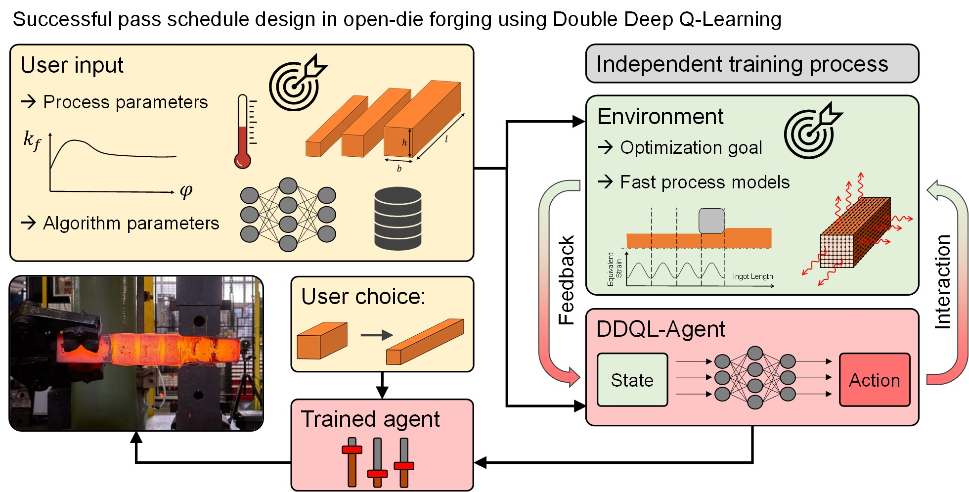
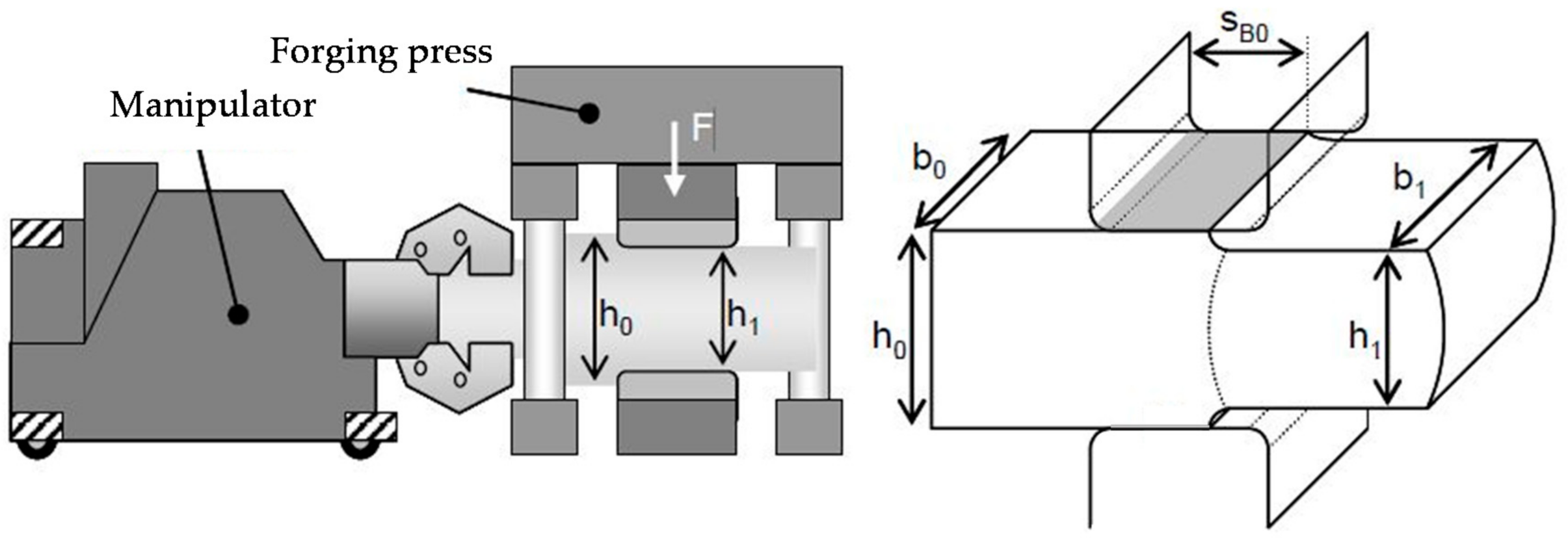
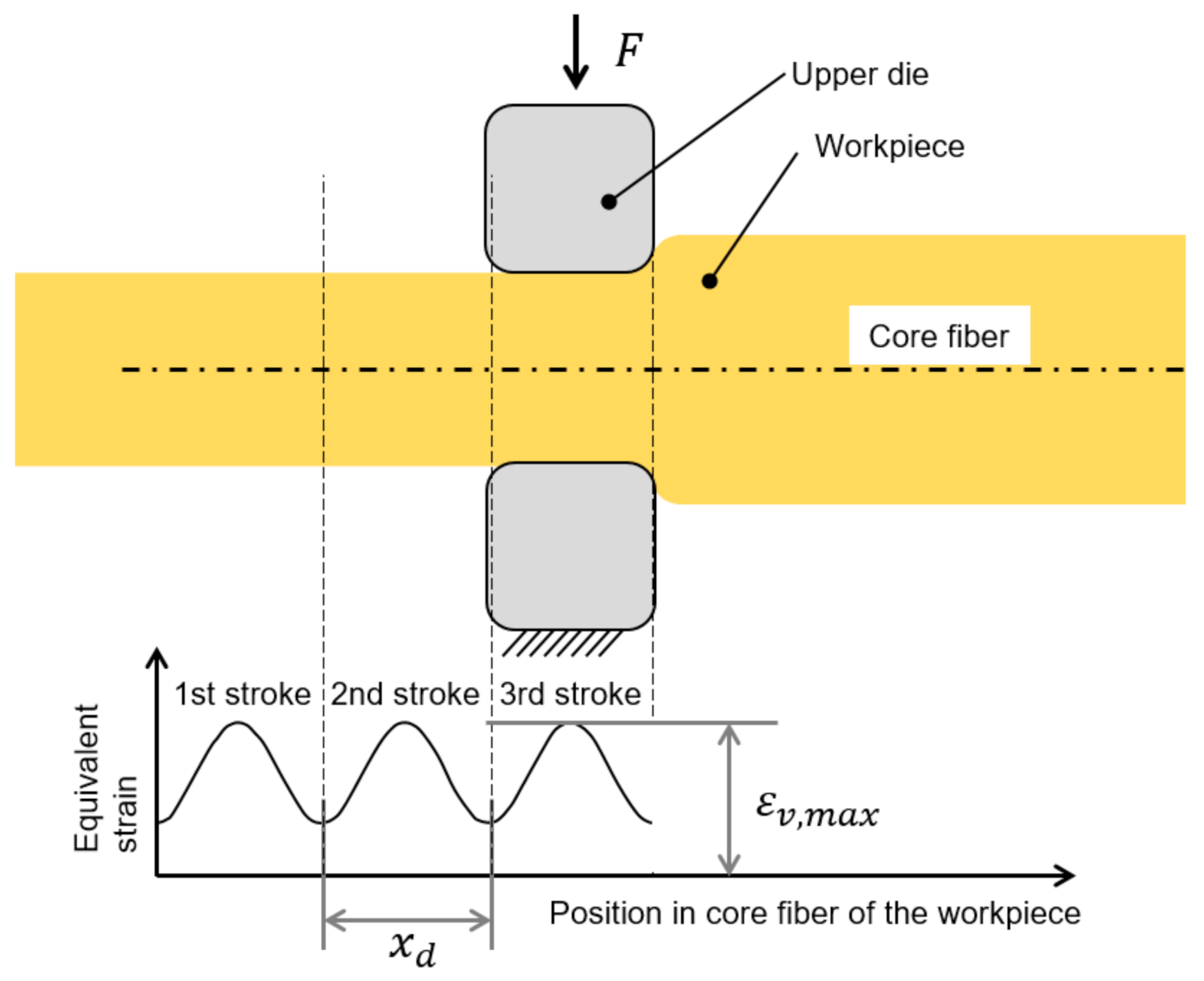
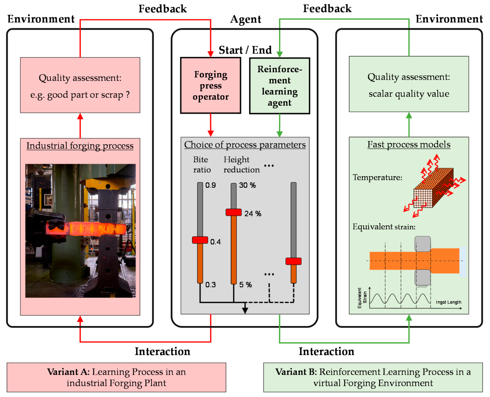
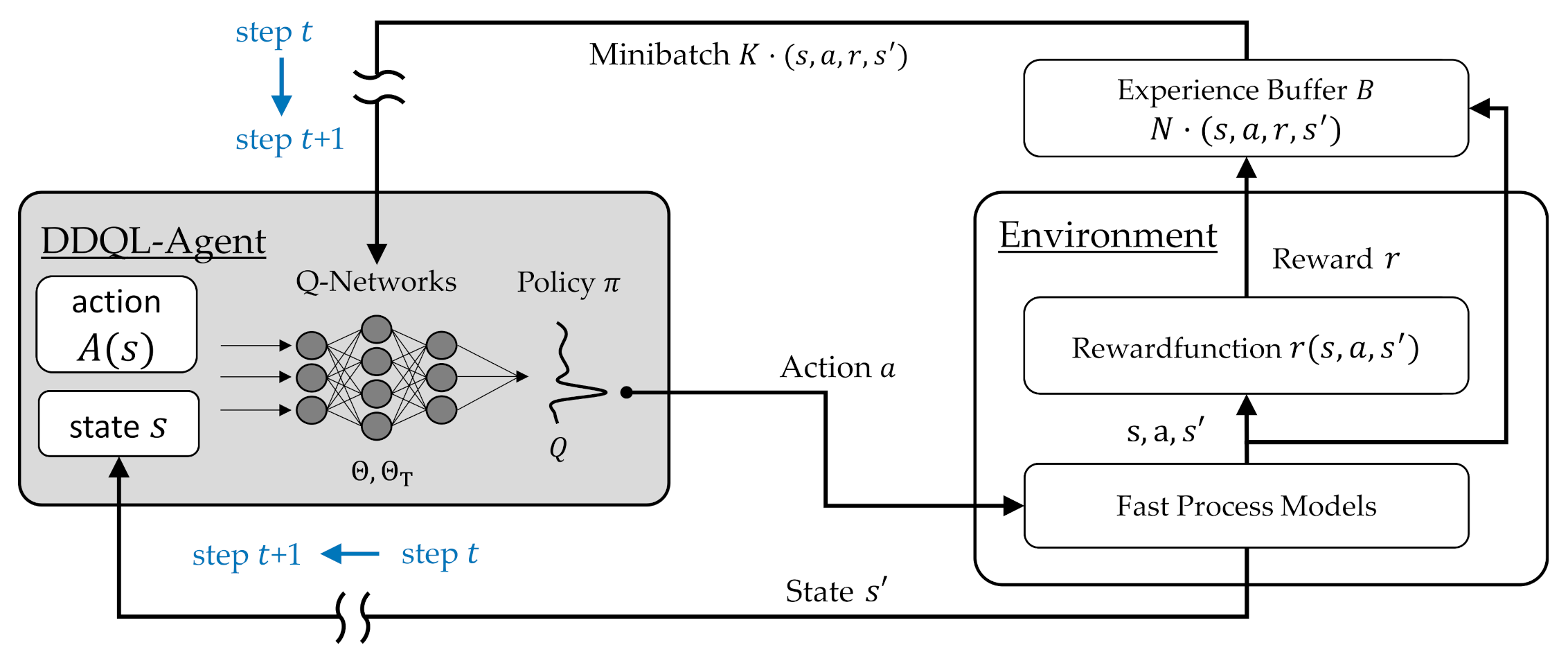
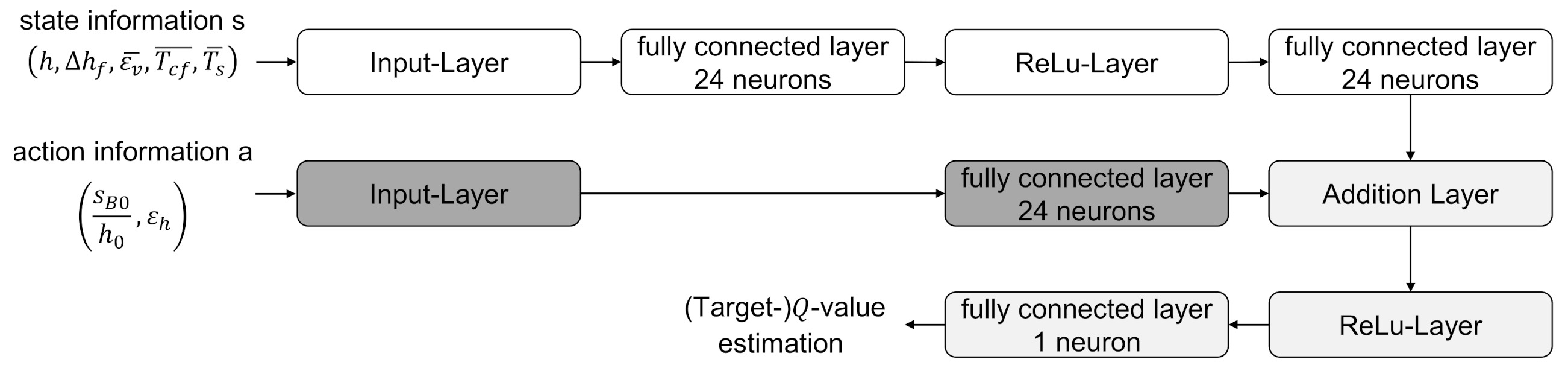
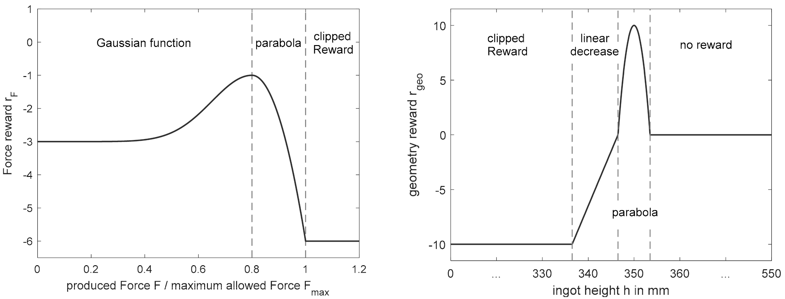
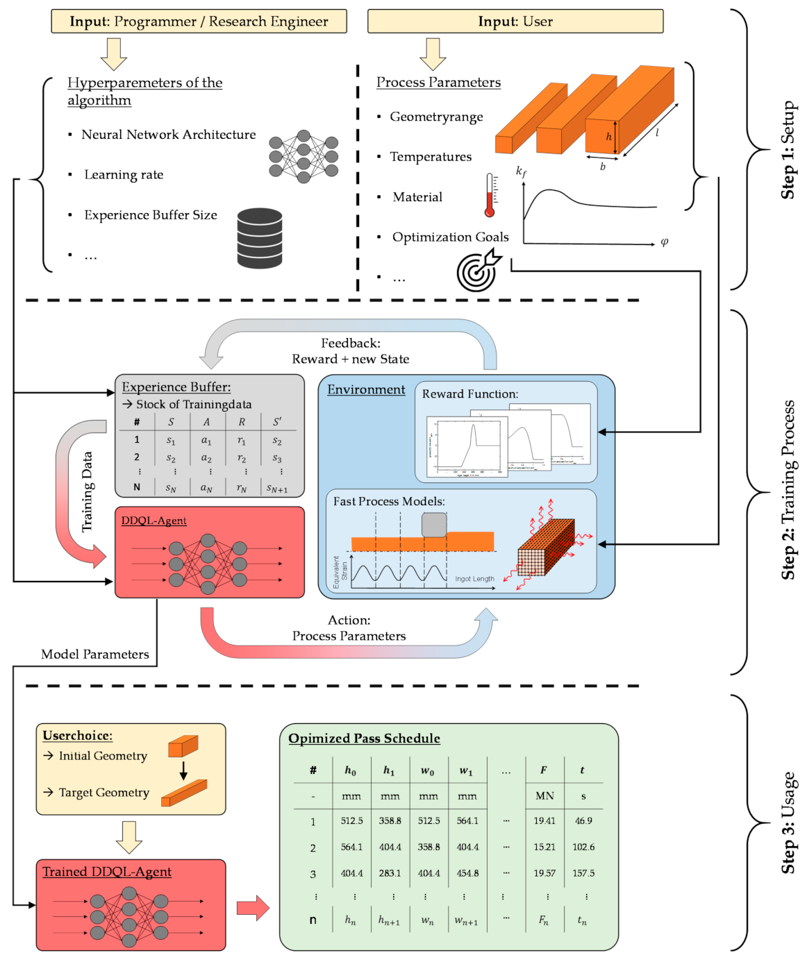
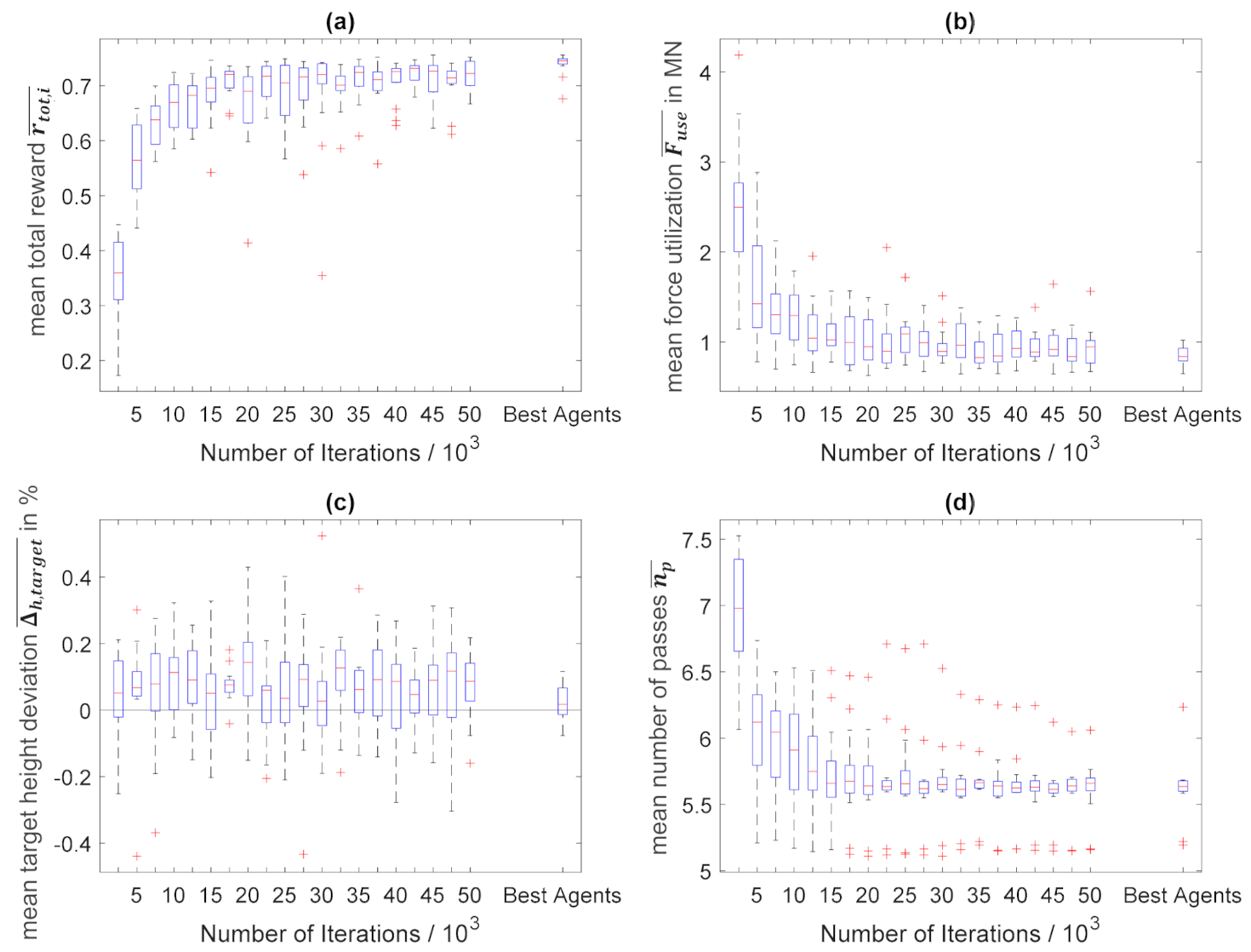
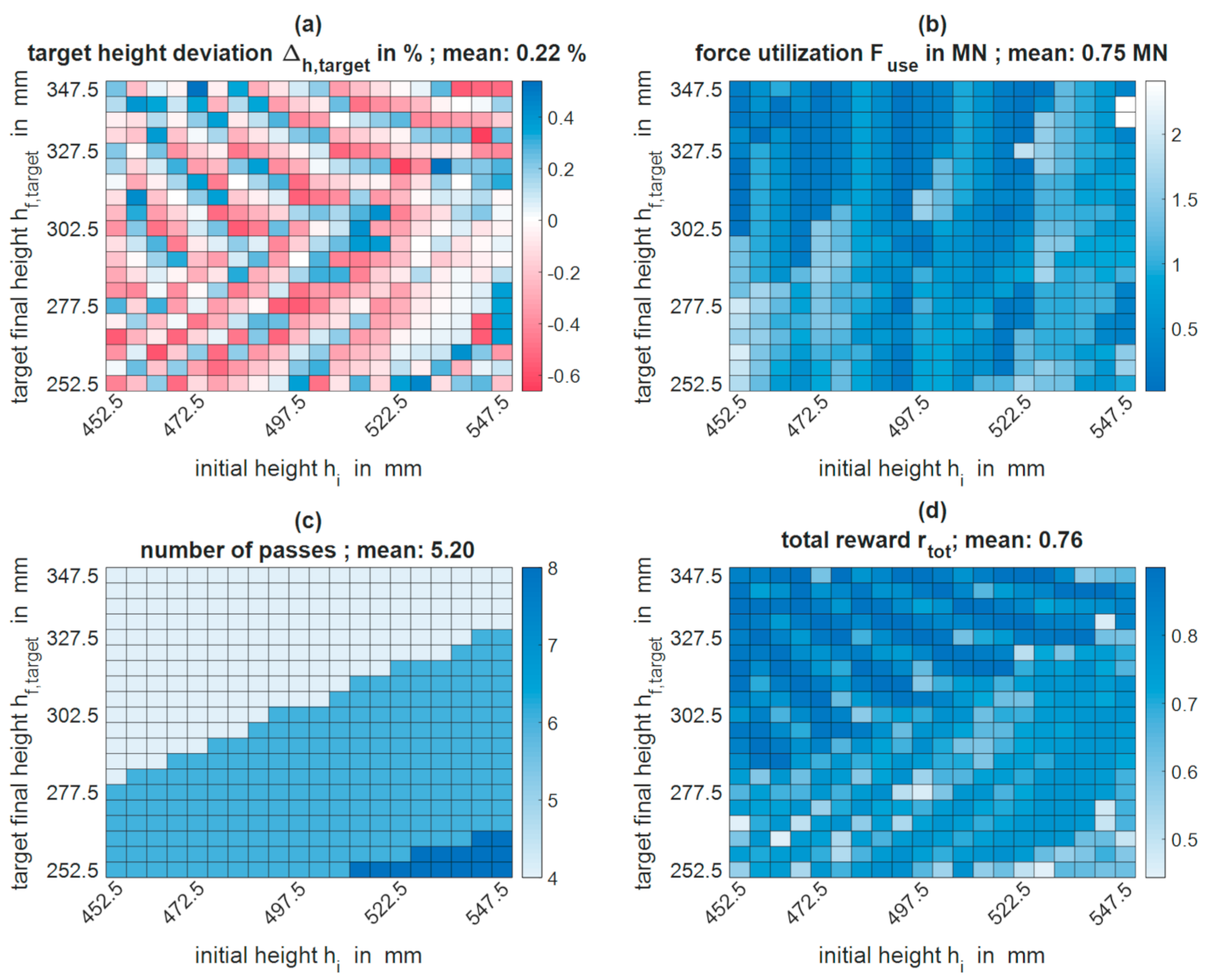
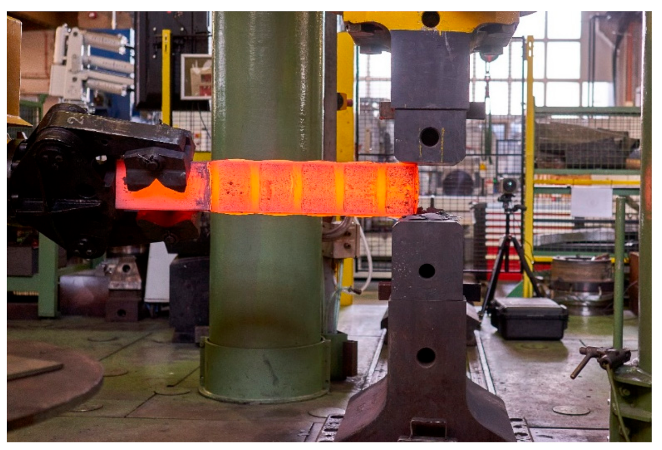
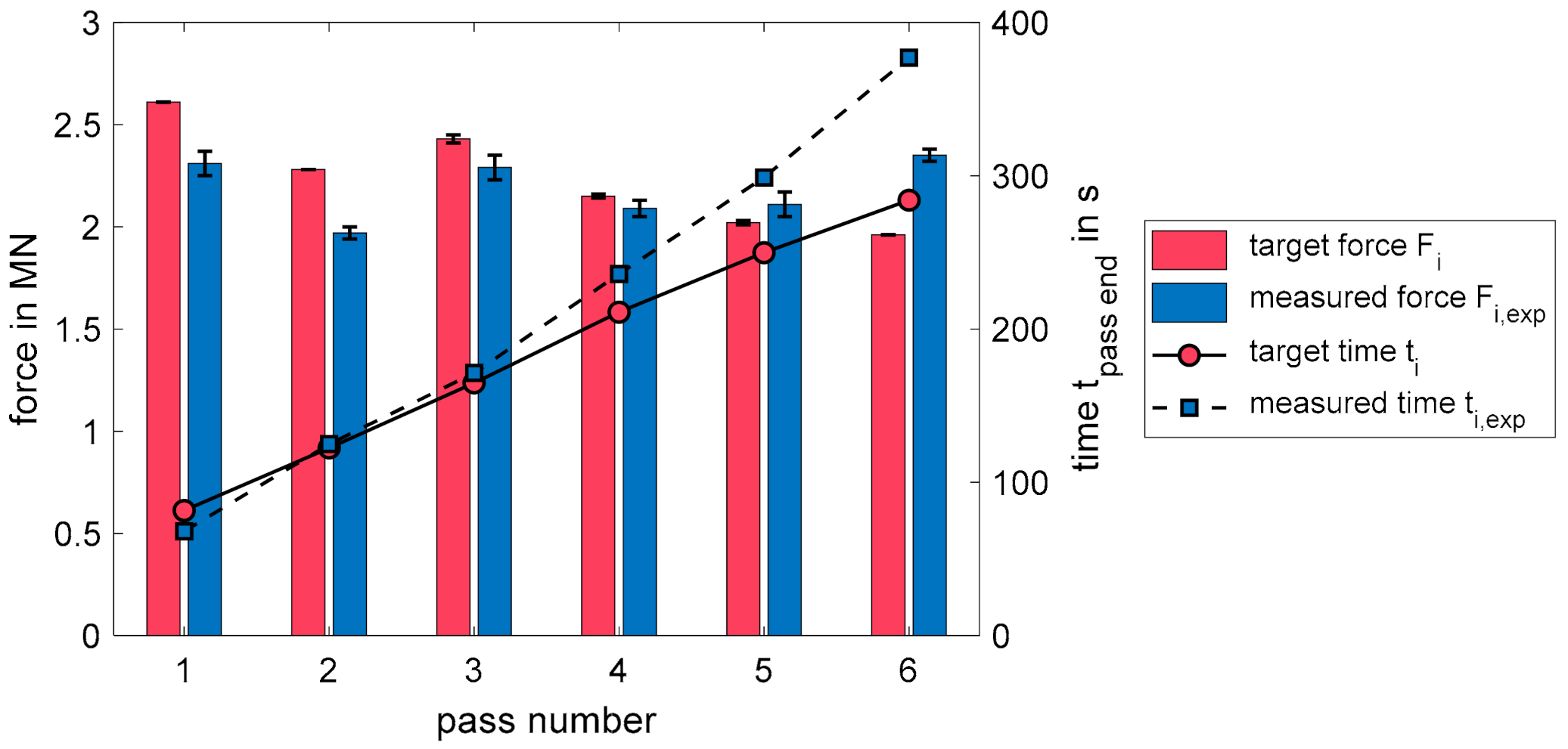
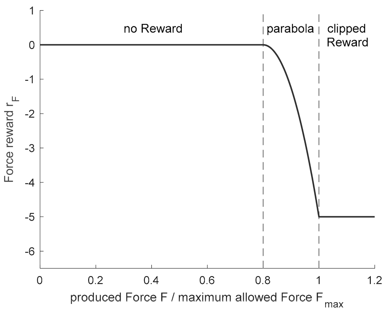
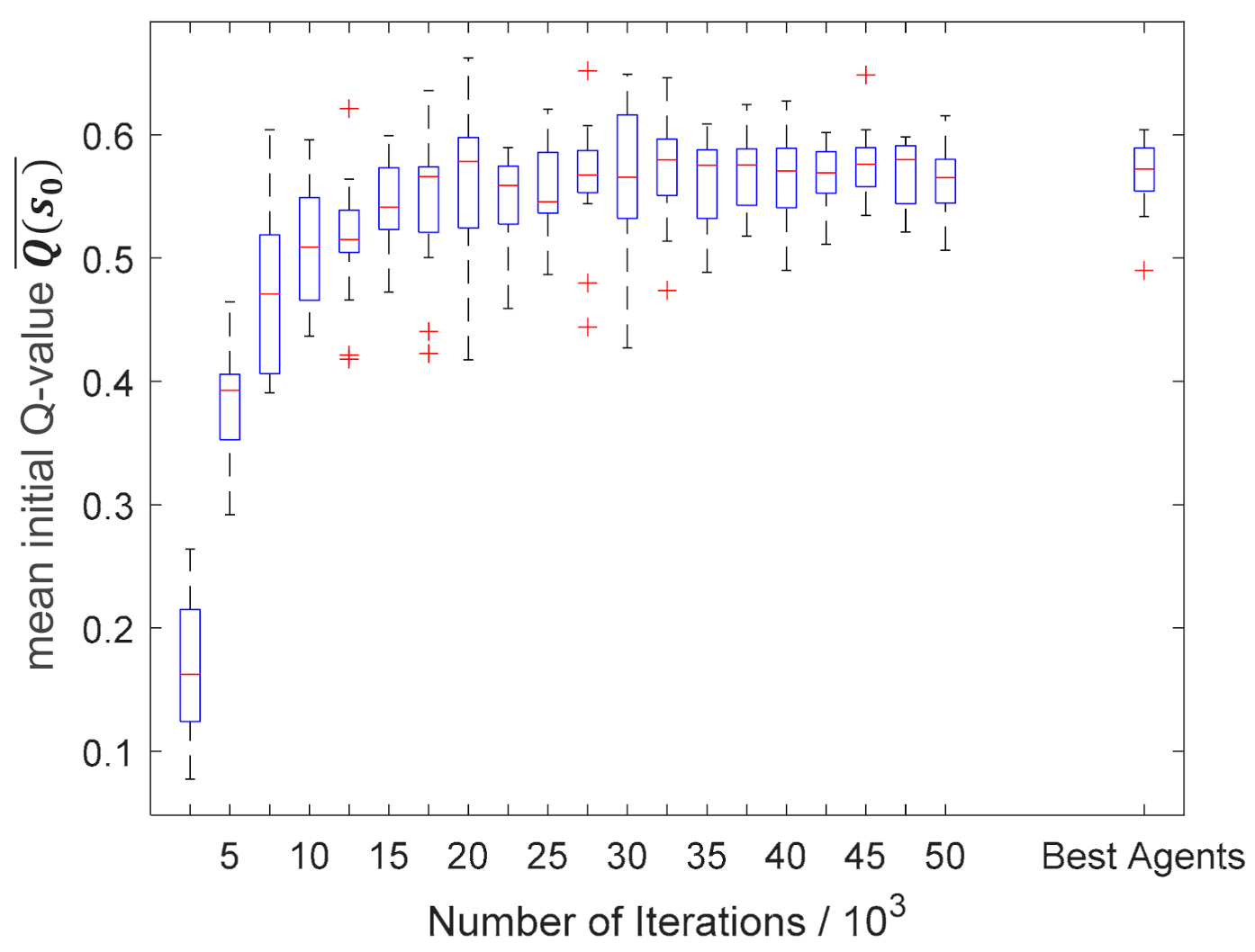
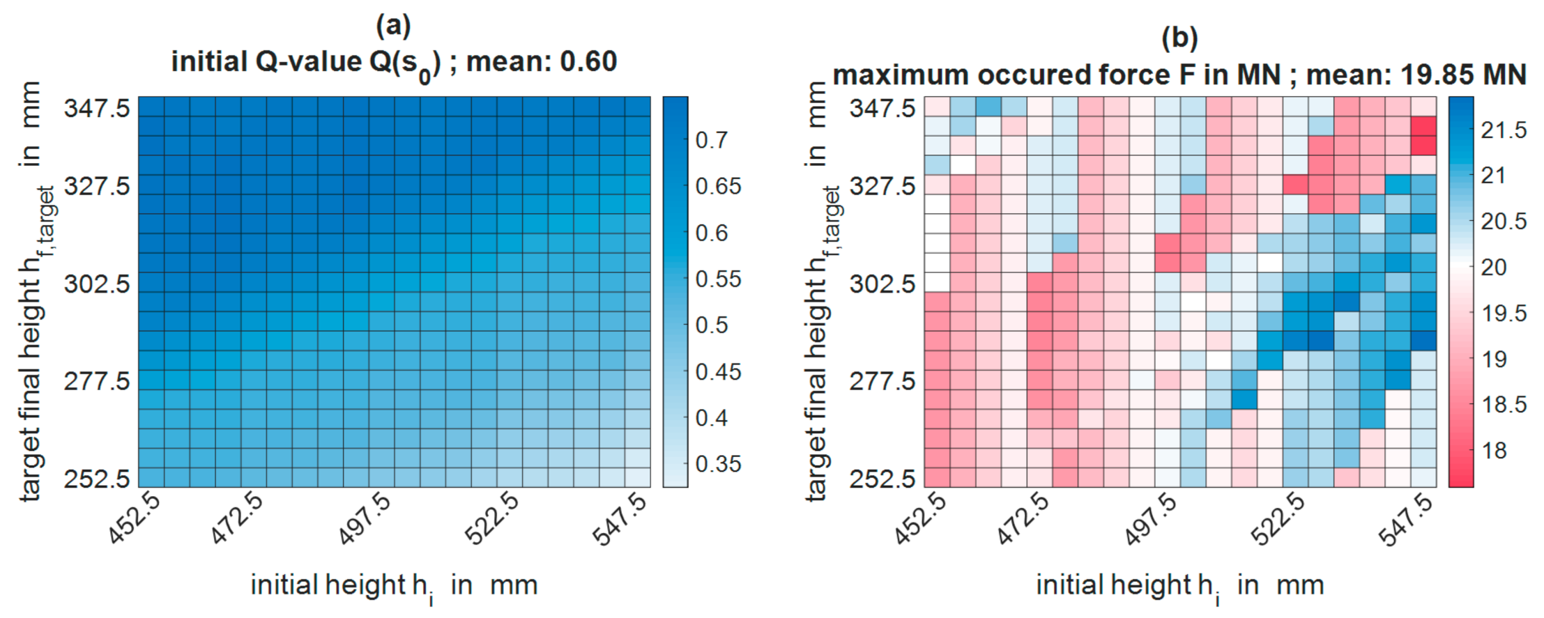
Table 1.
Tomlinson and Stringer parameters for 42CrMo4 [23].
Table 1.
Tomlinson and Stringer parameters for 42CrMo4 [23].
| Model | ||||
|---|---|---|---|---|
| Tomlinson Stringer, 2 parameters | 0.160 | 0.260 | 0 | 3.9% |
| Tomlinson Stringer, 3 parameters | 0.130 | 0.377 | −0.075 | 2.0% |
Table 2.
Material parameters used in temperature model for 1.7725 [25].
Table 2.
Material parameters used in temperature model for 1.7725 [25].
| °C | W/(m × K) | J/(kg*K) | kg/m3 |
| 800 | 23.44 | 697.1 | 7570.5 |
| 900 | 26.14 | 694.6 | 7517.4 |
| 1000 | 27.87 | 692.1 | 7461.9 |
| 1100 | 29.21 | 689.6 | 7404.2 |
| 1200 | 30.60 | 687.2 | 7344.4 |
1 thermal conductivity.
Table 3.
Empiric parameter for 1.7225 [23].
Table 3.
Empiric parameter for 1.7225 [23].
| 0.2 | 0.3 | 0.4 | 0.6 | 0.6 | 0.95 | 1.1 | 1.3 | 1.6 | |
| 1.294 | 1.030 | 0.730 | 0.452 | 0.325 | 0.344 | 0.303 | 0.234 | 0.174 |
Table 4.
The pass schedule example generated using the overall best agent (training 15, iteration 45,000).
Table 4.
The pass schedule example generated using the overall best agent (training 15, iteration 45,000).
| Pass Number | Initial Height | Final Height | Initial Width | Final Width | Initial Length | Final Length | Height Reduction | Bite Ratio | Bite Length |
|---|---|---|---|---|---|---|---|---|---|
| - | mm | mm | mm | mm | mm | mm | % | - | mm |
| Total | 512.5 | 267.5 | 512.5 | 267.5 | 1500 | 5505.9 | 3–30 | 0.3–0.9 | - |
| 1 | 512.5 | 358.8 | 512.5 | 564.1 | 1500 | 1946.7 | 30 | 0.4 | 205.0 |
| 2 | 564.1 | 404.4 | 358.8 | 404.4 | 1946.7 | 2409.0 | 28.3 | 0.4 | 225.7 |
| 3 | 404.4 | 283.1 | 404.4 | 454.8 | 2409.0 | 3059.8 | 30 | 0.6 | 242.6 |
| 4 | 454.8 | 327.8 | 283.1 | 327.8 | 3059.8 | 3667.7 | 27.9 | 0.6 | 272.9 |
| 5 | 327.8 | 245.8 | 327.8 | 350.8 | 3667.7 | 4568.4 | 25 | 0.3 | 98.3 |
| 6 | 350.8 | 266.6 | 245.8 | 266.6 | 4568.4 | 5542.0 | 24 | 0.3 | 105.3 |
| Time Stamp 1 | Rotation Angle 1 | Number of Strokes | Forging Direction | Tool Speed | Mean Temperature 1 | Min. Temperature 1 | Reheat 1 | Maximum Force | Mean Force |
| s | ° | - | - | mm/s | °C | °C | - | MN | MN |
| 470.3 | - | - | feed | - | 1000 | 1000 | - | - | - |
| 46.9 | 90 | 8 | feed | 100 | 993.7 | - | - | 19.41 | 19.11 |
| 102.6 | 90 | 9 | feed | 100 | 986.6 | 732.0 | no | 15.21 | 14.31 |
| 157.5 | 90 | 10 | feed | 100 | 979.2 | - | - | 19.57 | 18.52 |
| 226.4 | 90 | 12 | feed | 100 | 968.3 | 661.5 | no | 14.41 | 14.31 |
| 346.1 | 90 | 37 | feed | 100 | 946.2 | - | - | 9.16 | 7.05 |
| 470.3 | 90 | 44 | feed | 100 | 922.0 | 598.3 | yes | 8.32 | 6.10 |
1 At the end of the pass.
Table 5.
Pass schedule of the experiment, generated with the adapted and retrained algorithm.
| Pass Number | Initial Height | Final Height | Initial Width | Final Width | Initial Length | Final Length | Height Reduction | Bite Ratio | Bite Length |
|---|---|---|---|---|---|---|---|---|---|
| - | mm | mm | mm | mm | mm | mm | % | - | mm |
| Total | 150 | 100 | 150 | 100 | 500 | 1125 | 3–25 | 0.3–0.9 | - |
| 1 | 150 | 112.5 | 150 | 165.6 | 500 | 603.9 | 25 | 0.65 | 97.5 |
| 2 | 165.6 | 126.6 | 112.5 | 126.6 | 603.9 | 701.4 | 23.5 | 0.65 | 107.6 |
| 3 | 126.6 | 96.3 | 126.6 | 139.7 | 701.4 | 836.6 | 24 | 0.7 | 88.7 |
| 4 | 139.7 | 108.1 | 96.3 | 108.1 | 836.6 | 961.9 | 22.6 | 0.7 | 97.8 |
| 5 | 108.1 | 94.1 | 108.1 | 114.3 | 961.9 | 1046.3 | 13 | 0.85 | 91.9 |
| 6 | 114.3 | 99.9 | 94.1 | 99.9 | 1046.3 | 1126.3 | 12.5 | 0.85 | 97.1 |
| Time Stamp 1 | Rotation Angle 1 | Number of Strokes | Forging Direction | Tool Speed | Mean Temperature 1 | Minimum Temperature 1 | Reheat 1 | Maximum Force | Mean Force |
| s | ° | - | - | mm/s | °C | °C | - | MN | MN |
| 284 | - | - | feed | - | 1050 | 1000 | - | - | - |
| 81.6 | 90 | 5 | feed | 50 | 972.7 | - | - | 2.79 | 2.61 |
| 122.4 | 90 | 6 | feed | 50 | 935.5 | 710.7 | no | 2.51 | 2.28 |
| 164.8 | 90 | 8 | feed | 50 | 900.4 | - | - | 2.72 | 2.43 |
| 211 | 90 | 9 | feed | 50 | 864.7 | 658.6 | no | 2.53 | 2.15 |
| 249.8 | 90 | 11 | feed | 50 | 832.9 | - | - | 2.33 | 2.02 |
| 284 | 90 | 11 | feed | 50 | 805.7 | 622.1 | yes | 2.31 | 1.96 |
1 At the end of the pass.
Table 6.
Overview of the expected and measured averaged forces and their standard deviations.
| Pass Number | Evaluated Strokes | Time Difference 1 | ||||
|---|---|---|---|---|---|---|
| - | - | MN | MN | MN | MN | s |
| 1 | 2–4 | 2.61 | 0.00 | 2.31 | 0.06 | −13.6 |
| 2 | 2–5 | 2.28 | 0.00 | 1.97 | 0.03 | 2.5 |
| 3 | 2–7 | 2.43 | 0.02 | 2.29 | 0.06 | 6.5 |
| 4 | 2–8 | 2.15 | 0.01 | 2.09 | 0.04 | 24.9 |
| 5 | 2–9 | 2.02 | 0.01 | 2.11 | 0.06 | 49.1 |
| 6 | 3–9 | 1.96 | 0.00 | 2.35 | 0.03 | 93 |
1 Between the generated pass schedule and real experiment at the end of each pass.
Publisher’s Note: MDPI stays neutral with regard to jurisdictional claims in published maps and institutional affiliations. |
© 2021 by the authors. Licensee MDPI, Basel, Switzerland. This article is an open access article distributed under the terms and conditions of the Creative Commons Attribution (CC BY) license (https://creativecommons.org/licenses/by/4.0/).
Share and Cite
MDPI and ACS Style
Reinisch, N.; Rudolph, F.; Günther, S.; Bailly, D.; Hirt, G. Successful Pass Schedule Design in Open-Die Forging Using Double Deep Q-Learning. Processes 2021, 9, 1084. https://0-doi-org.brum.beds.ac.uk/10.3390/pr9071084
AMA Style
Reinisch N, Rudolph F, Günther S, Bailly D, Hirt G. Successful Pass Schedule Design in Open-Die Forging Using Double Deep Q-Learning. Processes. 2021; 9(7):1084. https://0-doi-org.brum.beds.ac.uk/10.3390/pr9071084
Chicago/Turabian StyleReinisch, Niklas, Fridtjof Rudolph, Stefan Günther, David Bailly, and Gerhard Hirt. 2021. "Successful Pass Schedule Design in Open-Die Forging Using Double Deep Q-Learning" Processes 9, no. 7: 1084. https://0-doi-org.brum.beds.ac.uk/10.3390/pr9071084
Note that from the first issue of 2016, this journal uses article numbers instead of page numbers. See further details here.