Demand Forecasting for Multichannel Fashion Retailers by Integrating Clustering and Machine Learning Algorithms

Abstract

In today’s rapidly changing and highly competitive industrial environment, a new and emerging business model—fast fashion—has started a revolution in the apparel industry. Due to the lack of historical data, constantly changing fashion trends, and product demand uncertainty, accurate demand forecasting is an important and challenging task in the fashion industry. This study integrates k-means clustering (KM), extreme learning machines (ELMs), and support vector regression (SVR) to construct cluster-based KM-ELM and KM-SVR models for demand forecasting in the fashion industry using empirical demand data of physical and virtual channels of a case company to examine the applicability of proposed forecasting models. The research results showed that both the KM-ELM and KM-SVR models are superior to the simple ELM and SVR models. They have higher prediction accuracy, indicating that the integration of clustering analysis can help improve predictions. In addition, the KM-ELM model produces satisfactory results when performing demand forecasting on retailers both with and without physical stores. Compared with other prediction models, it can be the most suitable demand forecasting method for the fashion industry.

1. Introduction

The fashion industry has evolved and greatly transformed in the past two decades [1,2]. The current developing trend is to vertically integrate the supply chain to shorten the response time and quickly respond to customer needs. The fashion industry supply chain has also changed from the traditional push production to pull production, and product inventory has dropped considerably. The fast-changing and highly competitive industrial environment has made fast fashion an important business model, setting off an affordable fashion trend around the world.

In the fast fashion industry, accurate demand forecasting is an important and challenging task due to uncertain product demand and extremely short product life cycles. In the past, many models have already been proposed to solve the forecasting problem of the fashion industry. The methods generally used to construct demand forecasting models include traditional statistical and machine learning methods [3]. Among them, traditional statistical methods such as the autoregressive integrated moving average model (ARIMA) or the grey method (GM) have shown good predictive performances in many studies [4,5]. However, as pointed out in previous studies [6], the fashion industry has highly complex data patterns, which makes it difficult for traditional statistical methods to produce good prediction results. Compared with traditional statistical methods, machine learning methods such as support vector regression (SVR) and extreme learning machines (ELMs) have been successfully applied to many sales and demand forecasting studies without the need for model assumptions [7,8,9,10,11].

In the past, a common way to construct prediction models was to put all training data into the model construction stage at once. However, putting data with different characteristics into the model can likely produce inaccurate prediction results, so the cluster-based hybrid prediction model is often used to improve predictions. As clustering can reduce the degree of data heterogeneity, it helps improve the accuracy of predictions [11,12,13]. The usage of ELM and SVR further shortens the time needed to process highly complex demand data for the fashion industry and model construction. Therefore, this research proposes two fast fashion industry demand forecasting models based on clustering analysis: the prediction model that integrates k-means (KM) and ELM (the KM-ELM prediction model) and the prediction model that integrates KM and SVR (the KM-SVR prediction model) to meet the fast fashion industry needs of demand forecasting.

There are very few cluster-based machine learning prediction models that are applied to demand forecasting of the fast fashion industry in the past. The framework proposed in this study not only uses the historical sales data commonly used in forecasting related literature as a predictor variable [9,14] but also adds meteorological data as a predictor variable to improve the accuracy of forecasting in the fashion industry. To verify the effectiveness of the KM-ELM and KM-SVR forecasting models proposed in this study, we compared the performances of the simple ELM, simple SVR, proposed KM-ELM, and proposed KM-SVR models when predicting the demand of fashion retailers with and without physical stores.

This paper is organized as follows. The first section is the introduction. Section 2 analyzes existing literature. Furthermore, we discuss and analyze techniques used in this study, including KM, ELM, and SVR. Section 3 provides details on the research method, explaining the research framework, process of data collection and processing, and construction process of each model. Section 4 is empirical analysis, going through the analytical data of the models using the process discussed in Section 3. Finally, we conclude this study in Section 5.

2. Literature Review

2.1. Demand Forecasting in the Fashion Industry

Accurate demand forecasting can increase the profitability of retailers by improving the operational efficiency of the supply chain and minimizing waste; inaccurate forecasting will lead to excessive or insufficient inventory, which will affect the retailer’s profitability and competitive position [15]. The main concept of the fast fashion industry is to continuously provide fashionable products to the market, reflect the latest fashion trends, and grasp the most popular designs currently on the market [6]. As a result, the fast fashion industry has some unique characteristics, including the lack of historical data, demand uncertainty, and short-term sales seasons [2].

Many studies in the past are dedicated to solving the problem of demand forecasting. Traditional statistical models have short computation times; for instance, the ARIMA model can build hundreds of historical data points in a few seconds to complete a time series forecast [16]. However, statistical methods may not perform well when the data patterns are highly complex. Previous studies [17] have pointed out that many artificial intelligence algorithms can be used to estimate nonlinear relationships. As an example, artificial neural networks (ANN) are often used in sales forecasting [3]. In the related research of fast moving consumer goods, a previous study [18] used ANN to predict the sales of women’s clothing. Another previous study [19] applied ENN to the sales forecast of the fashion retail industry. Although ANN and ENN models are widely used in forecasting, they require a lengthy model-building process.

In [3], a new model called the intelligence fast sales forecasting model was proposed, which used an ELM and traditional statistical methods such as polynomial regression. It suggested to use the extended extreme learning machine (ELM) when the time cost does not exceed the limit, and use the statistical prediction model when it does.

Integration of GM and extended ELM method (EELM) was performed in [6] to form the 3F algorithm. The study concluded that, in a limited time, the conversion of the 3F algorithm to GM can provide fast forecast results; if the time limit is not exceeded, then the GM-EELM model is used to perform the task of predicting.

2.2. K-Means Clustering

The main goal of clustering is to divide the collected sample data into several clusters. Data in the same cluster exhibit higher similarity, while the similarity between data in different clusters is low. KM clustering, a partitioning method, was proposed in [20], and it has been widely used in clustering operations [21,22] for cluster analysis because of its simple concept, easy operation, and fast computation time. In addition, KM applied to forecasting also yields good performance. In [12], KM and a greedy algorithm were combined to propose a KGA model for finding the optimal number of nodes in the hidden layer of a back-propagating neural network. Studies have confirmed that the model has good prediction accuracy. In [13], a new hybrid method that combined KM and a nonlinear autoregressive (NAR) neural network to predict the total amount of solar radiation per hour was proposed. Studies have confirmed that this method has better prediction performance than the autoregressive moving average (ARMA) model.

2.3. Extreme Learning Machines

ELMs were proposed in [23], which is a machine learning method [24,25,26,27]. It is noted that ELM is a single-hidden layer feedforward neural network, and its learning speed is faster than traditional gradient learning methods [6]. The study in [28] further explains that the construction of the network is through an acyclic feedforward connection that connects three-layer units, where the hidden layer is used to capture the relationship between the nonlinear input and output. Traditional learning methods need to adjust the input weight and the deviation of the hidden layer, but the input weight and hidden layer deviation in ELM can be randomly generated, which helps avoid the difficulties faced when using gradient learning algorithms such as poor learning rate, local minimums, and overfitting [3,28,29]. ELM has successfully solved prediction problems in many fields. The study [7] used ELMs to forecast sales in the fashion retail industry and indicated that ELMs outperformed other forecasting methods and back-propagation neural networks in this empirical context. Similar to fast fashion retailing demand, accurate price forecasting for electricity and crude oil is an arduous task owing to high volatility of the real-life data. ELM-based methods have been successfully applied in the cases where their advantages of faster learning speed with a higher generalization were taken and then highlighted. For example, in [30], wavelet transform and an ELM were combined to develop a hybrid wavelet based ELM (WELM) model that can be employed to electricity price forecasting. Empirical results confirmed that wavelet-ELM has good forecasting performance in price forecasting. The study in [10] used an ensemble empirical mode decomposition combined with extended ELM to predict the highly volatile price of crude oil. This model is better than simply using EELM or other ensemble learning models, and significantly improves prediction performance.

2.4. Support Vector Regression

SVR is a machine learning technique developed based on the principle of structural risk minimization [31]. In [32], SVR is used to forecast the sales of newspapers and magazines, as well as obtaining an accurate forecast result.

Support vector machines (SVMs) are a machine learning method that was developed based on structural risk minimization in statistical learning theory [31]. The study in [33] mentions that SVMs are linear learning machines, implying that a linear function is always used to solve regression problems. When dealing with nonlinear regression problems, the input vector is transformed into a high-dimensional feature space using a nonlinear mapping function, and a linear regression is constructed on the feature space. A previous study [34] lists many kernel functions of a support vector machine. The radial type (RBF) kernel function should be the priority choice for the core function because the RBF kernel function has many great characteristics. First, it can classify nonlinear and high-dimensional data; second, it only needs to adjust C and two parameters, reducing the operational difficulty. The final output data range between 0 and 1, and the reduction of the range of data can reduce the computation time [35]. However, there are some cases where the RBF kernel function is not applicable. In particular, when the number of features is very large, only linear kernel functions can be used [35].

In [33], fuzzy theory was combined with SVM to predict the demand for perishable agricultural products. The research results show that the prediction accuracy of an SVM is better than that of the radial basis function neural network. The study in [36] combined the invasive weed optimization (IWO) algorithm and SVR to develop the IWO-SVR model and applied it to the prediction of oxygen supply. The results show that IWO-SVR has higher prediction accuracy than SVR.

According to the above-mentioned studies, an effective supply strategy of short-lived and quickly exhausted products is highly relied on accurate demand forecasting. SVMs can find the global minima of structural risks in given training data and perform well due to great generalizability in forecasting demand for agriculture perishable goods as well as oxygen supply, and thus they are believed to be suitable for fast-fading fashion products.

3. Proposed Clustering-Based Demand Forecasting Model

3.1. Proposed Scheme

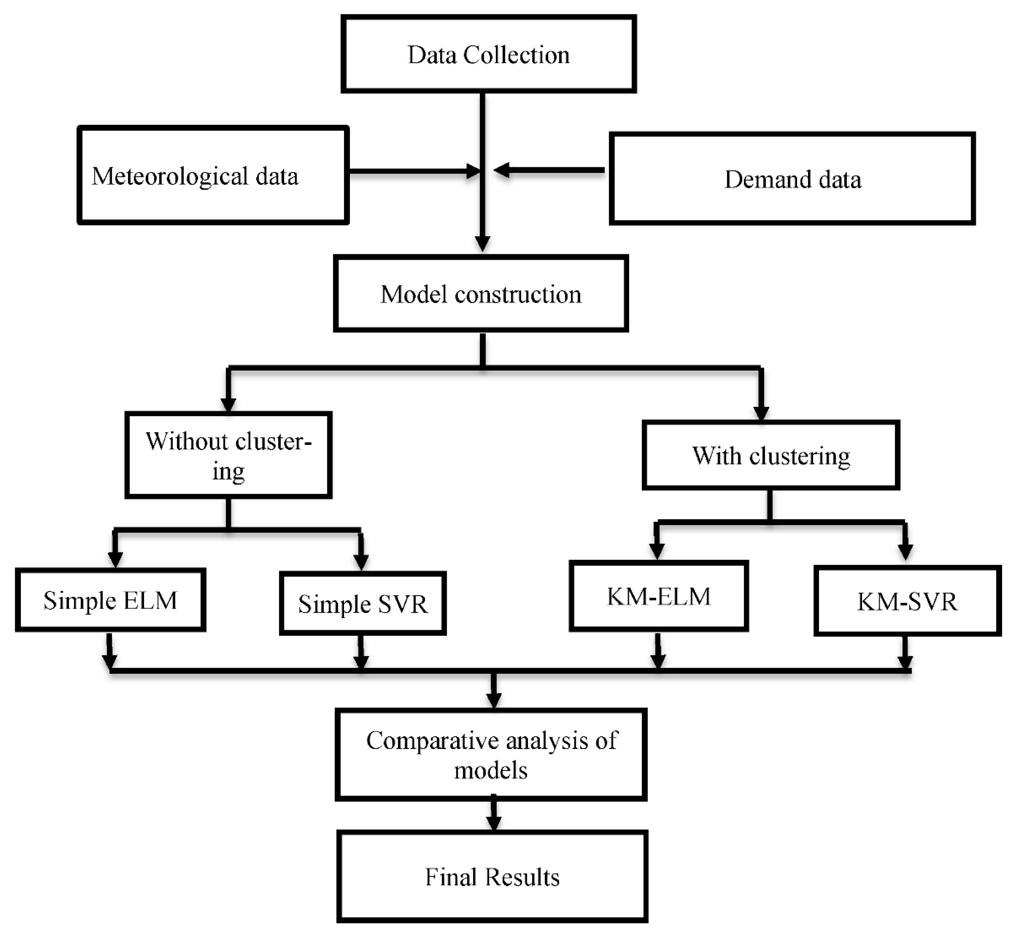
This study integrates clustering algorithm and machine-learning technique to propose a clustering-based forecasting model for fast fashion retailers to forecast the demand of physical store and non-store channel, respectively. The procedure is shown in Figure 1. According to the sales reviews on the FAST RETAILING website (https://www.fastretailing.com), past historical demand data and weather data, such as temperature and rainfall, are all important factors that affect the current demand particularly for physical stores. Therefore, this study collects two time series data of demand for physical and non-store channel.

However, most of the existing studies that focused on fashion demand forecasting have directly used all training data to construct models without considering the extent of the relevance between the training data and the data to be forecasted (test data) [6]. In such cases, forecasting accuracy may be reduced because the training data possibly contain excessive data irrelevant to the test data, thereby increasing training errors. To reduce computational time and obtain promising forecasting performance, several recent studies have proposed using clustering algorithms to divide the whole forecasting data into multiple clusters having consistent data characteristics before constructing forecasting models of time series data [9,11,14].

While constructing this proposed clustering-based demand forecasting model, the main aim in the training phase is to divide the overall training data by predictor variables into multiple small training data partitions, each of which has its own peculiar consistent data characteristics, and then to train individual forecasting models for different clusters. That is, for N clusters, N forecasting models are trained. In the testing phase, the average linkage method based on Euclidean distance is applied to measure the similarity between the test data and every given cluster. The membership of an observation of test dataset to the specified cluster is determined by the minimal distance. The predicted value of the test data is obtained using the trained forecasting model corresponding to the cluster it belongs to. To put it in a nutshell, the five steps of modelling procedure are summarized as follows:

(1)

Data collection: Collect raw data and divide those data into training and testing data sets with a ratio of approximately 9:1.

(2)

Data clustering: Group the training data through the KM algorithm.

(3)

Cluster assignment: Calculate the Euclidean distance between each point of the test data and each training data cluster center and determine the training data cluster corresponding to each test datum by finding the shortest distance to make predictions.

(4)

Model building, assessment, and assignment: Combine the machine learning method ELM or SVR to establish a prediction model for each cluster. Determine the best forecasting technology for each group according to performance indicators.

(5)

Explainability: Propose an explanation based on the results of the KM-ELM and KM-SVR prediction models.

3.2. Collecting and Processing Data

This study uses data from UNIQLO, a leading brand in fast fashion, for empirical analysis. The demand data are taken from UNIQLO’s monthly sales report, and the sales data can also reflect the quantity of customer demand at the same period. In principle, physical stores are classified into two types when a retailer assesses the company’s financial performance: same-stores, which have been run for a full business year at least, and new stores, which are newly running under 1 business year. Our research defines same-store net demand as the net demand volume generated by the same-store; physical stores net demand is the sum of the net demand of same-stores and new stores; non-store net demand refers to the sum of direct mail and internet demand. In the 2019 business year, for example, the same-store net demand is the demand generated by the same-store in the previous business year (i.e., 1 September 2018–31 August 2019); the net demand of directly-operated stores is the sum of the same-stores’ net demand and the demand of new stores operating for less than one year (1 September 2018–31 August 2019). The demand data shown in the report are the monthly percentage change over the previous year, so this study defines the same-store net demand percentage as the same-store net demand change rate over the same period last year; non-store net demand percentage is the rate of change of non-store net demand compared to the same period last year. We will refer to these data as the rate of change of same-store net demand and non-store net demand, respectively. The definitions of the focal variables are expressed in following equations:

$$\mathrm{Total} \mathrm{number} \mathrm{of} \mathrm{physical} \mathrm{stores}=Q\left(S\right)+W(N)$$

(1)

where Q(S) indicates the number of stores that have been run more than 1 year (at the time being recruited in this study), referred to as same-stores and denoted as S; W(N) indicates the number of stores that have been run less than 1 year, referred to as new-stores and denoted as N.

$$\mathrm{Physical} \mathrm{channel} \mathrm{net} \mathrm{demand}={{\displaystyle \sum }}_{i=1}^q{S}_{it}+{{\displaystyle \sum }}_{j=1}^w{N}_{jt}$$

(2)

where $S_{it}$ represents the net demand in business year t generated by the i^th same-store, $i=1\dots q$; $N_{jt}$ represents the net demand in business year t generated by the j^th new-store $j=1\dots w.$

$$\mathrm{Non}-\mathrm{store} \mathrm{channel} \mathrm{net} \mathrm{demand}=I_t+M_t$$

(3)

where $I_t$ represents the net demand in business year t generated by the Internet and $M_t$ represents the net demand in business year t generated by direct mail.

The source of the temperature and rainfall data for this study is the Japan Meteorological Agency. The prefectures with the largest number of physical stores of the case fashion company in the six regions of Japan are summarized in

Table 1. The top six number of physical stores in the corresponding six Japanese regions.

Number of Physical Stores	Prefecture	Region	City
108	Tokyo	Kantō	Tokyo
73	Osaka	Kansai	Osaka
48	Aichi	Chūbu	Nagoya
33	Fukuoka	Kyūshū·Okinawa	Fukuoka
29	Hokkaido	Hokkaidō·Tōhoku	Sapporo
19	Hiroshima	Shikoku·Chūgoku	Hiroshima

Source: Japan Meteorological Agency.

. Since temperature or rainfall varies with different regions and even is inconsistent in a very small geographical area, the main city of region is considered as the representative weather observatory due to the detailed temperature and rainfall figures unavailable for a specific area where a physical store is located.

3.3. Performance Evaluation Metrics

A good prediction method must have good accuracy. In this study, mean absolute percentage error (MAPE) and root mean squared error (RMSE), the two of most widely used measures of forecast accuracy [37,38], are used as the performance metrics. With merits of scale-independence and interpretability, MAPE can be comparable across different models or research for various magnitudes. With merits of scale-independence and interpretability, MAPE can be comparable across different models or research for various magnitudes. MAPE is classified into four levels [39]. When MAPE is less than 10%, it implies that the error between the actual and predicted values is considerably small and the model has excellent predictive ability.

Rather, RMSE penalizes larger errors by giving heavier weights since errors are squared before being averaged. RMSE is deemed to lay more stress on cost of undesirable deviations. The smaller the values of MAPE and RMSE, the more accurate the prediction model [37,38,39]. The performance evaluation formulas are as follows:

(1)

MAPE:

$$\mathrm{MAPE}=\frac{1}{n}\times {\displaystyle \sum _{\mathrm{i}=1}^{\mathrm{n}}\left|\frac{{\mathrm{T}}_{\mathrm{i}}-{\mathrm{F}}_{\mathrm{i}}}{{\mathrm{T}}_{\mathrm{i}}}\right|}\times 100\%$$

(4)

(2)

RMSE:

$$\mathrm{RMSE}=\sqrt{\frac{1}{\mathrm{n}}\times {\displaystyle \sum _{\mathrm{i}=1}^{\mathrm{n}}{\left({\mathrm{T}}_{\mathrm{i}}-{\mathrm{F}}_{\mathrm{i}}\right)}^2}}$$

(5)

where T_i is the actual value, and F_i is the predicted value.

A comparative analysis of resulting performances of all forecasting models in this study is accordingly conducted on these two criteria to alleviate the prejudice of either of metrics likely suffering.

4. Empirical Analysis

4.1. Empirical Data

The research data comprise two time series: monthly demand datasets of physical store channel and non-store channel separately, retrieved from annual financial statements of the case company for 12 years from September 2006 to August 2019 and then respectively computed by their definitions in Section 3.2. There are 156 observations in each retailing channel. In addition to the endogenous monthly demand data, the exogenous meteorological data are temperature and rainfall of the six regions taken as well on the monthly basis. Every region also has 156 points in either of temperature or rainfall datasets. To examine the applicability and generalization of the proposed clustering-based machine learning forecasting models, KM-SVR and KM-ELM, for demand of fast fashion retailers, the first 144 data points are used as the training sample, while the remaining 12 data points (the last year of sampled period) are holdout and are used as the testing sample for out-of-sample forecasting. The results of the proposed forecasting models on testing sample are compared with those of benchmarking models based on a single machine learning algorithm such as simple SVR and simple ELM. A model with the smallest RMSE/MAPE of the testing sample is chosen as the one more suitable for the case of the fast fashion industry than others for demand forecasting applied in this paper.

This study uses KM clustering in the IBM SPSS Statistics 22 software package to construct a cluster-based model. Subsequently, the program packages elmNN and e1071 in version 3.2.3 of R software (R core team, Vienna, Austria) are used to establish the ELM and SVR prediction models for each cluster.

4.2. Predictor Variables

This empirical study aims to propose clustering-based demand forecasting algorithms for fast fashion industry, which is expected to be characterized by short-lived products, insufficient historical data of newly launched merchandise, and uncertain demand over different phases of product life cycle. To alleviate the insufficiency of short-term data, decisions on what predictor variables should be included in forecasting model is very crucial to the accuracy of prediction results.

The predictor variables employed in this study have been extensively examined and their advantageous outcomes have been shown in the related literature [9,11,14,16,18,19]. In other words, this research is enlightened to include not merely 10 endogenous variables of monthly demand but also exogenous weather variables such as the temperature and rainfall of the region a retailer store is located in. It is also worth noting that the BIAS indicators, which have been verified to increase predicting accuracy in related studies [9,14,40], are served as the 3-of-10 endogenous variables with attempts to improve the forecasting performance.

Here, four issues can be addressed by the manipulation of whether; 10 endogenous variables of the two different time series, physical store and non-store channels’ demand datasets, can be incorporated well with the 14 weather variables in the simple ELM, simple SVR, KM-SVR, and KM-ELM models. Through such different combinations of predictor variables selected as inputs or not, an effective forecasting model for a given channel demand can be identified by its better resulting accuracy than those of the other models. In brief, Issue 1 is designated to forecast physical channel demand using 10 variables (X1_P to X10_P), compared with 24 variables (X1_P to X24) in Issue 2. In the same vein, issue 3 is for the non-store channel using 10 variables (X1_N to X10_N) while issue 4 involves 24 variables (X1_N to X24).

Table 2. Predictor variables.

	Issue	Issue 1	Issue 2	Issue 3	Issue 4
Variables		Physical Stores Demand	Physical Stores Demand with Meteorological Data	Non-store Demand	Non-Store Demand with Meteorological Data
Endogenous variables	(X1) Rate of change in the last month (t-1)	X1_P	X1_P	X1_N	X1_N
	(X2) Rate of change in the last two months (t-2)	X2_P	X2_P	X2_N	X2_N
	(X3) Rate of change in the last six months (t-6)	X3_ P	X3_ P	X3_N	X3_N
	(X4) Rate of change of the same month of last year (t-12)	X4_ P	X4_ P	X4_N	X4_N
	(X5) Moving average of the rate of change in the past two months (MA2)	X5_p	X5_ P	X5_N	X5_N
	(X6) Moving average of the rate of change in the past three months (MA3)	X6_P	X6_P	X6_N	X6_N
	(X7) Moving average of the rate of change in the past six months (MA6)	X7_P	X7_P	X7_N	X7_N
	(X8) BIAS of the last two months (BIAS2)	X8_P	X8_P	X8_N	X8_N
	(X9) BIAS of the rate of change of the last three months (BIAS3)	X9_P	X9_P	X9_N	X9_N
	(X10) BIAS of the rate of change of the same store of the last six months (BIAS6)	X10_P	X10_P	X10_N	X10_N
Exogenous variable	(X11) Average temperature of Sapporo		X11		X11
	(X12) Average temperature of Nagoya		X12		X12
	(X13) Average temperature of Tokyo		X13		X13
	(X14) Average temperature of Osaka		X14		X14
	(X15) Average temperature of Hiroshima		X15		X15
	(X16) Average temperature of Fukuoka		X16		X16
	(X17) Average temperate of all six regions (average of X11 to X16)		X17		X17
	(X18) Average rainfall of Sapporo		X18		X18
	(X19) Average rainfall of Nagoya		X19		X19
	(X20) Average rainfall of Tokyo		X20		X20
	(X21) Average rainfall of Osaka		X21		X21
	(X22) Average rainfall of Hiroshima		X22		X22
	(X23) Average rainfall of Fukuoka		X23		X23
	(X24) Average rainfall of all six regions (average of X18 to X23)		X24		X24

Note: $\mathrm{MA}2=\frac{{{\displaystyle \sum }}_{i=1}^2\mathrm{change} \mathrm{rate} \mathrm{of} \mathrm{demand} \mathrm{in} \mathrm{month} \left(\mathrm{t}-\mathrm{i}\right) }{2}; \mathrm{MA}3=\frac{{{\displaystyle \sum }}_{i=1}^3 \mathrm{change} \mathrm{rate} \mathrm{of} \mathrm{demand} \mathrm{in} \mathrm{month} \left(\mathrm{t}-\mathrm{i}\right) }{3};$ $\mathrm{MA}6=\frac{{{\displaystyle \sum }}_{i=1}^6\mathrm{change} \mathrm{rate} \mathrm{of} \mathrm{demand} \mathrm{in} \mathrm{month} \left(\mathrm{t}-\mathrm{i}\right)}{6} ; \mathrm{BIAS}2=\frac{\mathrm{demand} \mathrm{of} \mathrm{month} \mathrm{t}-\mathrm{MA}2}{\mathrm{MA}2}$; $\mathrm{BIAS}3=\frac{\mathrm{demand} \mathrm{of} \mathrm{month} \mathrm{t}-\mathrm{MA}3}{\mathrm{MA}3}$; $\mathrm{BIAS}6=\frac{\mathrm{demand} \mathrm{of} \mathrm{month} \mathrm{t}-\mathrm{MA}6}{\mathrm{MA}6}$, where t is the current month.

summarizes predictor variables utilized for the four issues.

4.3. Results

This study uses ELM, SVR, KM-ELM, and KM-SVR models for demand forecasting to find the best prediction models between them. The former two models are served as the benchmarking for the latter two to examine the effectiveness of clustering-based machine learning algorithms we proposed. This study uses three activation functions—linear, sigmoid, and radial basis—in simple ELM and KM-ELM, and it uses radial and linear kernel functions in simple SVR and KM-SVR. The prediction results on physical stores and non-store channels are shown below.

The authors of [23] indicated that the most important ELM parameter is the number of hidden nodes, and ELM tends to be unstable in single run forecasting. Following the instructions of [11,40], the ELM models with different numbers of hidden nodes varying from 1 to 30 are constructed. For each number of nodes, an ELM model is repeated 10 times and the average RMSE and MAPE of each node is calculated. With an example of using simple ELM for Issue 1, through automation process of model computation, the best 6 results from the respective 6 amounts of hidden nodes are selected to emphasize in

Table 3. The number of hidden nodes and activation functions of ELMs and results for Issue 1.

Activation Function	Number of Hidden Nodes	MAPE	RMSE
Linear Transfer Function	10	0.44%	0.62
	18	0.44%	0.62
	19	0.44%	0.62
	20	0.44%	0.62
	21	0.44%	0.62
	22	0.44%	0.62
Sigmoid Transfer Function	10	9.11%	11.21
	18	7.60%	9.96
	19	7.96%	10.53
	20	8.27%	11.01
	21	9.02%	11.32
	22	7.29%	9.52
Radial Basis Transfer Function	10	57.20%	73.39
	18	99.99%	106.75
	19	91.97%	102.20
	20	85.82%	96.05
	21	77.47%	89.30
	22	88.61%	100.04

Note: boldface indicates the best result.

, for the sake of limited length. Table 3 compares 6 different number of nodes of ELM with 3 different activation functions using 10 predictor variables of physical channel. We find that simple ELM achieves its best performance when activation function is linear, and 10 hidden nodes are applied (MAPE = 0.44%, RMSE = 0.62) for Issue 1. The same procedure is used for all simple ELM and KM-ELM models for all four issues.

For modelling SVR, the grid search proposed by Hsu et al. [35] is a common and straightforward method using exponentially growing sequences of C (a correction coefficient) and ε (a loss function) to identify good parameters. Taking simple SVR for Issue 1 as example, this study tested 17 different combinations of parameters to find the best SVR model. When radial is used for the kernel function, the best-performing parameter combination incorporates a correction coefficient of 1.05, a loss function of 0.05, and a gamma of 0.6; when linear is used for the kernel function, the superior parameter combination has a correction coefficient of 1.05, a loss function of 0.03, and a gamma of 1.3. The results show that simple SVR predicts better when using a linear kernel function, with MAPE = 0.42% and RMSE = 0.59 for issue 1. The above procedure of finding best parameter set for simple SVR and KM-SVR models is used for all four issues.

4.3.1. Clustering-Based Prediction Model

Determining the number of clusters beforehand is a challenging task for analysts. While no perfect mathematical criterion exists, the many heuristics available appear to rely on the field where it is applied [41,42]. Prediction accuracy is one of common criteria to determine the optimal cluster number (here, the parameter K for K-means algorithm). For a retailing demand time series, K from 2 to 5 can obtain desirable clustering results [11,40,41].

Furthermore, by virtue of seasonal variation in demand for fashion products, the number of clusters is supposed to lie in 4 (seasons) or somewhere between 2 to 5 as well. Since prediction accuracy is a common criteria to determine the optimal cluster number [42], a clustering-based model that generates the highest accuracy is defined as the best forecasting model, suggesting the optimal number of clusters for this empirical case (Issue 2 and the later Issue 4). Hence, we take the experiment on the range of clusters between 2 and 5 using the 10 endogenous variables as the clustering variables.

Our study integrated KM with ELM as KM-ELM where different parameters were tweaked, such as the activation function, the number of nodes, and the number of clusters. We obtained 24 clustering-based models, as shown in

Table 4. Using different activation functions in KM-ELM and the results for physical channel (Issue 1).

	MAPE			RMSE
Activation Function/Number of Clusters	Linear	Sigmoid	Radial Basis	Linear	Sigmoid	Radial Basis
2	0.31%	6.72%	58.10%	0.38	9.02	73.80
3	0.25%	6.57%	60.55%	0.30	9.19	74.90
4	0.22%	5.73%	34.42%	0.27	7.5	46.80
5	0.13%	4.79%	42.68%	0.14	5.82	50.58

Note: boldface indicates the best result.

. The prediction accuracy of KM-ELM is highest when there are five clusters and linear activation function used in ELM (MAPE = 0.13%, RMSE = 0.14).

Table 5. Clustering results of the best KM-ELM (K = 5) for physical channel (Issue 1).

	Cluster 1	Cluster 2	Cluster3	Cluster 4	Cluster 5	Total
Training data	24	66	35	11	8	144
Testing data	2	5	3	1	1	12
Total	26	71	38	12	9	156

uncovers the data distributed across the 5 clusters of the best KM-ELM (K = 5).

Likewise, from

Table 6. Using different kernel functions in KM-SVR and the results for physical channel (Issue 1).

	MAPE		RMSE
Kernel Function/Number of Clusters	Radial	Linear	Radial	Linear
2	4.13%	0.33%	5.3	0.42
3	5.47%	0.21%	7.38	0.29
4	5.20%	0.24%	6.13	0.30
5	5.69%	0.23%	6.70	0.26

Note: boldface indicates the best result.

, we can see that when we apply SVR after KM clustering, using a linear kernel function yields better accuracy than using a radial kernel function for physical channel (Issue 1). The prediction accuracy is highest when there are three clusters for KM-SVR.

Table 7. Clustering results of best KM-SVR (K = 3) for physical channel (Issue 1).

	Cluster 1	Cluster 2	Cluster 3	Total
Training data	61	54	29	144
Testing data	5	5	2	12
Total	66	59	31	156

uncovers the data distributed across the 3 clusters of the best KM-SVR (K = 3).

4.3.2. Comparison of Prediction Models

The prediction results for physical channel (Issue 1 and 2) are summarized in

Table 8. Physical channel results with 10 and 24 predictor variables.

		ELM	SVR	KM-ELM	KM-SVR
10-predictor forecasting model (Issue 1)	MAPE	0.44%	0.42%	0.13%↓	0.21%↓
	RMSE	0.62	0.59	0.14↓	0.29↓
24-predictor forecasting model (Issue 2)	MAPE	0.70%	0.68%	0.50%↓	0.57%↓
	RMSE	0.80	0.73	0.64↓	0.68↓

Note: boldface indicates the best results and ↓ denotes the decreases compared with the benchmark models.

. In a mere comparison of pure algorithms, which are served as the benchmarking models, simple SVR produced lower MAPE and RMSE than those of simple ELM. More importantly, the proposed KM-ELM and KM-SVR achieved better prediction accuracy than simple ELM, and simple SVR. KM-ELM was the best model (MAPE = 0.13%↓, RMSE = 0.14↓) when performing demand forecasting for Issue 1 and Issue 2 of the physical channel. Similarly, when constructing non-store demand forecasting models for Issue 3 and Issue 4, KM-ELM still performed the best, though by a low margin. Although RMSE of KM-ELM in Issue 4 is higher than that of KM-SVR by 0.01, it still has the lowest MAPE, as shown in

Table 9. Non-store channel results with 10 and 24 predictor variables.

		ELM	SVR	KM-ELM	KM-SVR
10-predictor forecasting model (Issue 3)	MAPE	0.32%	0.42%	0.14%↓	0.26%↓
	RMSE	0.41	0.40	0.15↓	0.21↓
24-predictor forecasting model (Issue 4)	MAPE	0.31%	0.36%	0.25%↓	0.27%↓
	RMSE	0.40	0.40	0.23↓	0.22↓

Note: boldface indicates the best results and ↓ denotes the decreases compared with the benchmark models.

.

It implies that the proposed KM-ELM and KM-SVR methods are applicable and more effective for fast-fashion demand forecasting, regardless of retailing channels. Since fashion retailers periodically launch new products or remodel the existing merchandise on the markets to keep pace with the customer’s craze and sensation, they accordingly have to orchestrate their marketing campaigns in a timely manner for implementation of annual sales plans over different seasons. As a result, the demand of fashion products exhibits similar data patterns or features at different time periods. Aligned with the inference above, KM-ELM and KM-SVR can obtain promising forecasting performances by means of clustering the data in several groups to reduce the likelihood that a model learns the patterns irrelevant to the testing data in the training phase.

However, the accuracy declined slightly when the number of predictor variables increased in a model. This could be attributable to the curse of dimensionality, which is an interesting topic for future studies.

5. Conclusions

The effective operation of a retailer relies on demand forecasting more than other strategic and planning decisions. An accurate demand forecast can directly affect the company’s profitability and competitive advantage in the market. This study uses the demand data of fashion retailer’s physical and non-store channels as empirical data and constructs demand forecasting models through KM clustering combined with ELMs or SVR. The results show that KM-ELM and KM-SVR have higher prediction accuracy than the simple ELM and SVR prediction models. This verifies the position that, once data are sorted through clustering, the pre-processing of data homogenization can shorten the computational time needed to construct a model and help alleviate high complexity of demand data specific to the fashion industry. As a whole, clustering-based machine learning forecasting models can improve predictions under time pressure.

The fast fashion industry has uncertain product demand, extremely short product life cycles, and insufficient or incomplete historical data. However, constructing a forecasting model using machine learning requires high quality and sufficient data during the training process. Therefore, this study uses BIAS indicators, which are commonly used in time series measurement models, as predictor variables, and incorporates meteorological data as an attempt to compensate for the scarcity of data. It might be counterintuitive that the empirical results show the forecast results using 10 demand predictor variables to be more accurate than the forecast results using 24 demand predictor variables. We speculate that there are a few possible reasons for this. The empirical data used in this study are the rate of change in demand rather than the net demand and are the overall national demand rather than a local demand, which implies that they might not be affected by the climate of each specific region. Therefore, it is recommended that future researchers consider other external predictor variables such as holidays (school and business), commercially relevant events (Easter, Christmas), extraordinary events (e.g., a pandemic), and economic conditions when predicting demand for a more specific region or different sales channels. In addition, for the sake of obtaining more detailed managerial implications, interpretable machine learning algorithms can be the alterative methodology in future studies.

The results of this study show that the KM-ELM model is most suitable for demand forecasting in the fashion industry, and its superior forecasting ability makes it helpful for the operation and management of production and sales. Fast fashion companies can use the KM-ELM model even with limited data and under tight time constraints to obtain an accurate prediction result that is conducive to improving company performance management. This also enables fashion companies to achieve efficient and timely inventory management, which reduces inventory costs for retailers by lowering the probability of under- or overstocking.

References

- Frings, G.S. Fashion: From Concept to Consumer; Prentice-Hall: Englewood Cliffs, NJ, USA, 1982; p. 305. [Google Scholar]
- Nenni, M.E.; Giustiniano, L.; Pirolo, L. Demand Forecasting in the Fashion Industry: A Review. Int. J. Eng. Bus. Manag. 2013, 5, 37. [Google Scholar] [CrossRef] [Green Version]
- Yu, Y.; Choi, T.-M.; Hui, C.-L. An intelligent fast sales forecasting model for fashion products. Expert Syst. Appl. 2010, 38, 7373–7379. [Google Scholar] [CrossRef]
- Hossain, M.M.; Abdulla, F. Forecasting the garlic production in Bangladesh by ARIMA Model. Asian J. Crop Sci. 2015, 7, 147. [Google Scholar]
- Hsu, C.-C.; Chen, C.-Y. Applications of improved grey prediction model for power demand forecasting. Energy Convers. Manag. 2003, 44, 2241–2249. [Google Scholar] [CrossRef]
- Choi, T.-M.; Hui, C.-L.; Liu, N.; Ng, S.-F.; Yu, Y. Fast fashion sales forecasting with limited data and time. Decis. Support Syst. 2014, 59, 84–92. [Google Scholar] [CrossRef]
- Sun, Z.L.; Choi, T.M.; Au, K.F.; Yu, Y. Sales forecasting using extreme learning machine with applications in fashion re-tailing. Decis. Support Syst. 2008, 46, 411–419. [Google Scholar] [CrossRef]
- Lu, C.J.; Shao, Y.E. Forecasting computer products sales by integrating ensemble empirical mode decomposition and extreme learning machine. Math. Probl. Eng. 2012, 2012, 831201. [Google Scholar] [CrossRef]
- Lu, C.-J. Sales forecasting of computer products based on variable selection scheme and support vector regression. Neurocomputing 2014, 128, 491–499. [Google Scholar] [CrossRef]
- Yu, L.; Dai, W.; Tang, L. A novel decomposition ensemble model with extended extreme learning machine for crude oil price forecasting. Eng. Appl. Artif. Intell. 2016, 47, 110–121. [Google Scholar] [CrossRef]
- Chen, I.-F.; Lu, C.-J. Sales forecasting by combining clustering and machine-learning techniques for computer retailing. Neural Comput. Appl. 2016, 28, 2633–2647. [Google Scholar] [CrossRef]
- Tan, J.Y.B.; Bong, D.B.L.; Rigit, A.R.H. Time series prediction using backpropagation network optimized by Hybrid K-means-Greedy Algorithm. Eng. Lett. 2012, 20, 203–210. [Google Scholar]
- Benmouiza, K.; Cheknane, A. Forecasting hourly global solar radiation using hybrid K-means and nonlinear autoregressive neural network models. Energy Convers. Manag. 2013, 75, 561–569. [Google Scholar] [CrossRef]
- Lu, C.J.; Lee, T.S.; Lian, C.M. Sales forecasting for computer wholesalers: A comparison of multivariate adaptive regression splines and artificial neural networks. Decis. Support Syst. 2012, 54, 584–596. [Google Scholar] [CrossRef]
- Ramos, P.; Santos, N.; Rebelo, R. Performance of state space and ARIMA models for consumer retail sales forecasting. Robot. Comput. Manuf. 2015, 34, 151–163. [Google Scholar] [CrossRef] [Green Version]
- Murat, M.; Malinowska, I.; Gos, M.; Krzyszczak, J. Forecasting daily meteorological time series using ARIMA and regression models. Int. Agrophysics 2018, 32, 253–264. [Google Scholar] [CrossRef]
- Chen, S.; Chen, J. Forecasting container throughput at ports using genetic programming. Expert Syst. Appl. 2010, 37, 2054–2058. [Google Scholar] [CrossRef]
- Frank, C.; Garg, A.; Sztandera, L.; Raheja, A. Forecasting women’s apparel sales using mathematical modeling. Int. J. Cloth. Sci. Technol. 2003, 15, 107–125. [Google Scholar] [CrossRef] [Green Version]
- Au, K.-F.; Choi, T.-M.; Yu, Y. Fashion retail forecasting by evolutionary neural networks. Int. J. Prod. Econ. 2008, 114, 615–630. [Google Scholar] [CrossRef]
- MacQueen, J. Some methods for classification and analysis of multivariate observations. In Proceedings of the Fifth Berkeley Symposium on Mathematical Statistics and Probability, Berkeley, CA, USA, 21 June–18 July 1965; Volume 1, pp. 281–297. [Google Scholar]
- Guftar, M.; Ali, S.H.; Raja, A.A.; Qamar, U. A novel framework for classification of syncope disease using K-means clustering algorithm. In Proceedings of the 2015 SAI Intelligent Systems Conference (IntelliSys), London, UK, 10–11 November 2015; pp. 127–132. [Google Scholar]
- Xue, W.; Feijia, L.; Wenxia, X.; Kun, G.; Guodong, L. Based on K-Means Clustering and CNN Algorithm Research in Hail Cloud Determination. In Proceedings of the 2015 Seventh International Conference on Measuring Technology and Mechatronics Automation, Nanchang, China, 13–14 June 2015; pp. 232–235. [Google Scholar]
- Huang, G.-B.; Chen, L.; Siew, C.-K. Universal Approximation Using Incremental Constructive Feedforward Networks With Random Hidden Nodes. IEEE Trans. Neural Netw. 2006, 17, 879–892. [Google Scholar] [CrossRef] [Green Version]
- Benoît, F.; van Heeswijk, M.; Miche, Y.; Verleysen, M.; Lendasse, A. Feature selection for nonlinear models with extreme learning machines. Neurocomputing 2013, 102, 111–124. [Google Scholar] [CrossRef]
- Huang, G.; Song, S.; Gupta, J.N.D.; Wu, C. Semi-Supervised and Unsupervised Extreme Learning Machines. IEEE Trans. Cybern. 2014, 44, 2405–2417. [Google Scholar] [CrossRef]
- Kasun, L.L.C.; Zhou, H.; Huang, G.B.; Vong, C.M. Representational learning with extreme learning machine for big data. IEEE Intell. Syst. 2013, 28, 31–34. [Google Scholar]
- Huang, G.; Huang, G.B.; Song, S.; You, K. Trends in extreme learning machines: A review. Neural Netw. 2015, 61, 32–48. [Google Scholar] [CrossRef] [PubMed]
- Xia, M.; Lu, W.; Yang, J.; Ma, Y.; Yao, W.; Zheng, Z. A hybrid method based on extreme learning machine and k-nearest neighbor for cloud classification of ground-based visible cloud image. Neurocomputing 2015, 160, 238–249. [Google Scholar] [CrossRef]
- Huang, G.-B.; Zhu, Q.-Y.; Siew, C.-K. Extreme learning machine: Theory and applications. Neurocomputing 2006, 70, 489–501. [Google Scholar] [CrossRef]
- Shrivastava, N.A.; Panigrahi, B.K. A hybrid wavelet-ELM based short term price forecasting for electricity markets. Int. J. Electr. Power Energy Syst. 2014, 55, 41–50. [Google Scholar] [CrossRef]
- Vapnik, V.N. The Nature of Statistical Learning Theory; Springer, Inc.: New York, NY, USA, 1995. [Google Scholar]
- Yu, X.; Qi, Z.; Zhao, Y. Support Vector Regression for Newspaper/Magazine Sales Forecasting. Procedia Comput. Sci. 2013, 17, 1055–1062. [Google Scholar] [CrossRef] [Green Version]
- Du, X.F.; Leung, S.C.; Zhang, J.L.; Lai, K.K. Demand forecasting of perishable farm products using support vector machine. Int. J. Syst. Sci. 2013, 44, 556–567. [Google Scholar] [CrossRef]
- Gunn, S.R. Support vector machines for classification and regression. ISIS Tech. Rep. 1998, 14, 5–16. [Google Scholar]
- Hsu, C.W.; Chang, C.C.; Lin, C.J. A Practical Guide to Support Vector Classification; National Taiwan University: Taipei, Taiwan, 2003; pp. 1–16. [Google Scholar]
- Cai, X.; Nan, X.Y.; Gao, B.P. Oxygen supply prediction model based on IWO-SVR in bio-oxidation pretreatment. Eng. Lett. 2015, 23, 173–179. [Google Scholar]
- Kim, S.; Kim, H. A new metric of absolute percentage error for intermittent demand forecasts. Int. J. Forecast. 2016, 32, 669–679. [Google Scholar] [CrossRef]
- Willmott, C.; Matsuura, K. Advantages of the mean absolute error (MAE) over the root mean square error (RMSE) in assessing average model performance. Clim. Res. 2005, 30, 79–82. [Google Scholar] [CrossRef]
- Lewis, E.B. Control of body segment differentiation in drosophila by the bithorax gene complex. Prog. Clin. Biol. Res. 1982, 1, 269–288. [Google Scholar]
- Lu, C.J.; Chen, I.F. Identifying important predictors for computer server sales using an effective hybrid forecasting technique. Int. J. Inf. Manag. Sci. 2017, 28, 213–232. [Google Scholar]
- Lu, C.J.; Kao, L.J. A clustering-based sales forecasting scheme by using extreme learning machine and ensembling link-age methods with applications to computer server. Eng. Appl. Artif. Intell. 2016, 55, 231–238. [Google Scholar] [CrossRef]
- Jain, A.K. Data clustering: 50 years beyond K-means. Pattern Recognit. Lett. 2010, 31, 651–666. [Google Scholar] [CrossRef]