Turbulent Bubble-Laden Channel Flow of Power-Law Fluids: A Direct Numerical Simulation Study


1
Institute of Applied Mathematics and Scientific Computing, Bundeswehr University Munich, Werner-Heisenberg-Weg 39, 85577 Neubiberg, Germany
2
Multiscale Modeling and Simulation, Faculty EEMCS, University of Twente, P.O Box 217, 7500 AE Enschede, The Netherlands
*
Author to whom correspondence should be addressed.
Fluids 2021, 6(1), 40; https://0-doi-org.brum.beds.ac.uk/10.3390/fluids6010040
Submission received: 25 November 2020
/
Revised: 16 December 2020
/
Accepted: 18 December 2020
/
Published: 12 January 2021
(This article belongs to the Special Issue Modelling of Reactive and Non-reactive Multiphase Flows)
Abstract
:The influence of non-Newtonian fluid behavior on the flow statistics of turbulent bubble-laden downflow in a vertical channel is investigated. A Direct Numerical Simulation (DNS) study is conducted for power-law fluids with power-law indexes of 0.7 (shear-thinning), 1 (Newtonian) and 1.3 (shear-thickening) in the liquid phase at a gas volume fraction of 6%. The flow is driven downward by a constant volumetric flow rate corresponding to a friction Reynolds number of . The Eötvös number is varied between and in order to investigate the influence of quasi-spherical as well as wobbling bubbles and thus the interplay of the bubble deformability with the power-law behavior of the liquid bulk. The resulting first- and second-order fluid statistics, i.e., the gas fraction, mean velocity and velocity fluctuation profiles across the channel, show clear trends in reply to varying power-law indexes. In addition, it was observed that the bubble oscillations increase with decreasing power-law index. In the channel core, the bubbles significantly increase the dissipation rate, which, in contrast to its behavior at the wall, shows similar orders of magnitude for all power-law indexes.
1. Introduction
Turbulent bubble-laden channel flow plays an important role in a wide range of industrial applications, such as chemical reactors in the process industry, heat exchangers in power plants or boiling water reactors in the nuclear industry. Although many processes of practical interest can be considered as two-phase flows with Newtonian behavior in both phases, there is a large number of relevant applications where the continuous liquid phase exhibits non-Newtonian flow characteristics. Numerous examples can be found in the biomedical and biochemical, the metallurgical as well as the food-processing industries [1]. Common applications with bubbles moving in a non-Newtonian continuous phase are the degassing and devolatilization of polymer melts [2], the gas-assisted displacement of liquids in channels [3,4,5,6] as well as the utilization of bubble columns [7,8,9,10]. An extensive list of examples and previous investigations is provided by Chhabra [1], including some analytical, experimental and numerical studies of rise velocities and detailed velocity profiles for single bubbles and bubble chains in power-law fluids [11,12]. Many applications, such as the operation of bubble column reactors and purification processes using purge gases, are based on the heat and mass exchange between both phases. For these processes, it is beneficial if the bubbles make the maximum possible contact with the surrounding liquid. The bubble distribution and interface area are therefore key factors influencing the process efficiency. However, turbulence and the flow velocities also have a significant impact on the contact duration during which both phases can react or exchange mass and heat. Moreover, in processes with unwanted bubble generation, such as oil production, an accurate prediction of bubbly flow can help to improve the efficiency. It is therefore of great interest to analyze the dependency of the flow characteristics on the rheological behavior of the continuous liquid phase.
Since experimental investigations of bubbly flows remain challenging [13] and are often limited to dilute void fractions [14], DNS plays a major role in improving the fundamental understanding of the interaction between the continuous liquid phase and the dispersed bubbles. Due to the increased amount of computational resources available by now, DNS has become feasible for reduced-complexity two-phase flows at moderate Reynolds numbers. The pioneering numerical studies of Lu and Tryggvason [15,16,17] investigated the influence of different parameters on flows with up to 72 bubbles in the so-called minimum channel (see Section 3.2). While the computational cost and limited scalability restricted the applicability of DNS to rather simple setups for many years, recently developed massively parallel bubbly-flow solvers, such as the one used for this study [18,19], can efficiently handle up to fully deformable bubbles, while resolving all scales in DNS detail. Highly scalable DNS solvers for bubbly flow, which can simulate a large number of bubbles embedded in full-scale channels, offer the possibility to perform advanced evaluations, such as detailed investigations of flow topologies in dispersed bubbly flows [20,21].
Compared to the large number of studies investigating single-phase channel flow of Newtonian fluids, the effects of power-law based viscosity have rarely been investigated in this setup. Ohta and Miyashita [22] performed both single-phase DNS and Large Eddy Simulation (LES) to investigate wall turbulence for a channel setup similar to the one used in this study. To mimic the viscosity of general polymer solutions, both power-law as well as Casson fluids were used. The power-law indexes used in this study were 0.85 for the shear-thinning, and 1.15 for the shear-thickening fluid. The LES sub-grid scale stress was predicted by applying an extended Smagorinsky model.
This study extends the numerical investigation of turbulent channel flow of power-law fluids to two-phase downflow scenarios by including either quasi-spherical () or wobbling () bubbles. The number of bubbles is chosen such that the total gas fraction is at a technically relevant level of 6%. The shear-thinning and shear-thickening fluids are mimicked using power-law indexes of 0.7 and 1.3, respectively. The results are compared to those of single-phase simulations with identical power-law indexes as well as corresponding bubbly flow setups with a Newtonian liquid phase. This allows for studying both the effect the presence of a second phase exerts on the flow characteristics of the non-Newtonian continuous phase, as well as the influence of the rheological behavior in the continuous phase on the bubbles. For this purpose, the resulting viscosity profiles, average wall shear stresses, and first and second order fluid statistics are compared in the statistically steady state. In addition, the wall-normal profiles of the dissipation rate are provided for all investigated cases. Finally, the bubble deformation is quantified by investigating the average bubble surface area and its fluctuation.
The mathematical formulation of the power-law model determining the viscosity in the non-Newtonian continuous phase is provided in Section 2, the numerical method and the flow configuration are described in Section 3, and the results are presented and discussed in Section 4. Section 5 summarizes the findings and draws conclusions.
2. Mathematical Description of the Power-Law Model
In this study, the non-Newtonian continuous liquid phase obeys a power-law model for viscosity. The viscous stress tensor is defined as [23]
with the apparent viscosity , the consistency index K, the shear rate , the rate of strain tensor and the power-law index n. The apparent viscosity of the liquid phase, which is used to implement the power-law model in the solver, can therefore be expressed as
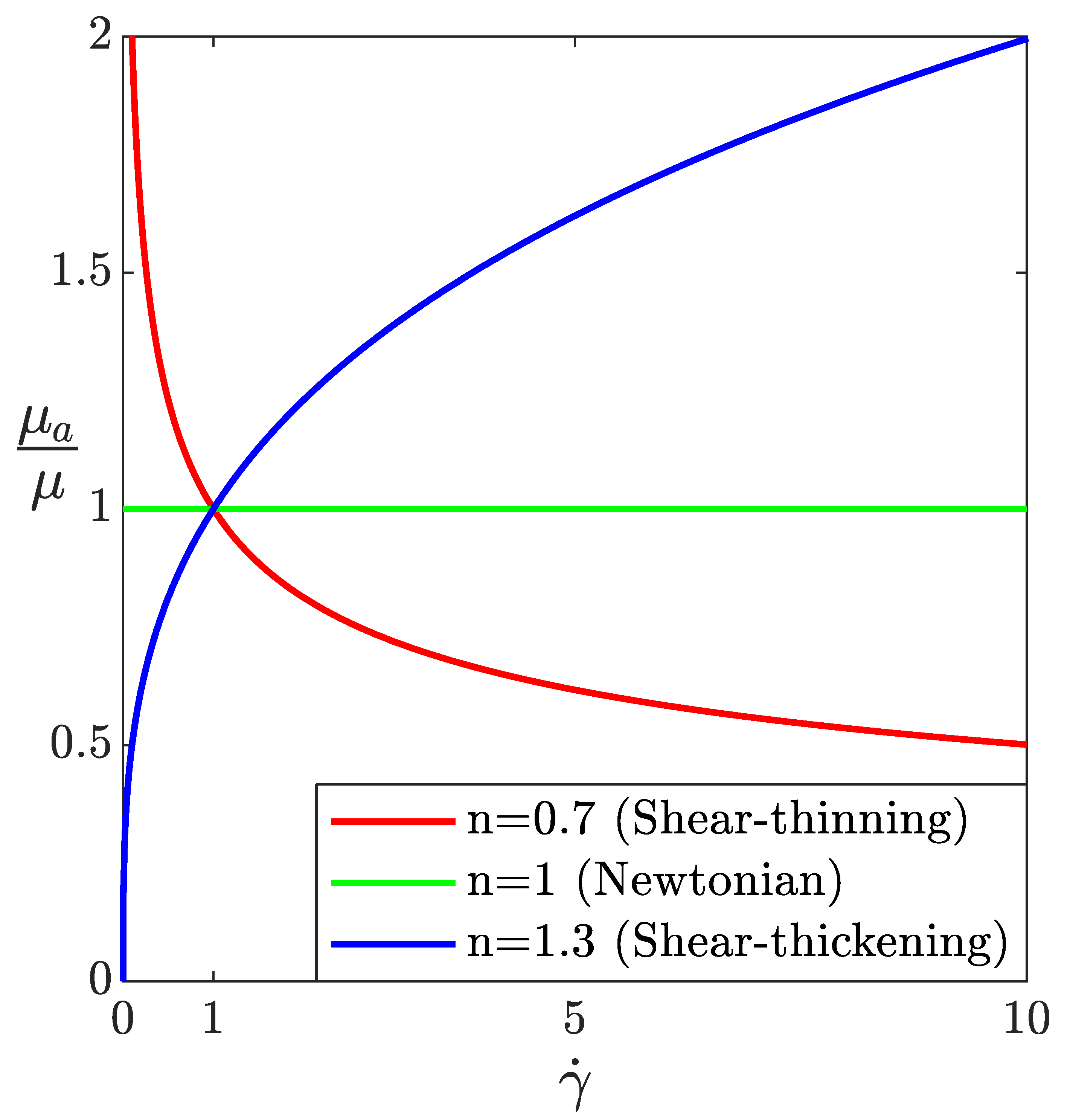
For shear-thinning fluids (), the apparent viscosity decreases with increasing shear rate, while the opposite effect occurs for shear-thickening fluids (). In this study, is not limited by a minimum or a maximum value. For Newtonian fluids (), the shear rate does not influence the apparent viscosity, which leads to . Figure 1 illustrates the dependency of the normalized apparent viscosity on the shear rate for the power-law indexes 0.7, 1, and 1.3, which are used in this study.
With only one free parameter, the power-law model provides the simplest possible relation between shear stress and shear rate for non-Newtonian fluids. Although the model has some limitations and does not represent all effects present in many real-world non-Newtonian fluids perfectly [1], its simplicity allows a straightforward analysis regarding the influence of shear rate dependent viscosity on the flow characteristics. The model implementation has been validated by comparing the wall-normal profile of the stream-wise velocity component resulting from a laminar single-phase test case to an analytical solution [24] for laminar two-dimensional channel flow of power-law fluids.
3. Numerical Method and Flow Configuration
3.1. Governing Equations and Numerical Framework
The mathematical model implemented in the highly scalable (hybrid openMP-MPI) open-source code “TBFsolver” [18] uses the one-fluid formulation [25] of the governing equations. It describes the entire flow field with a single set of equations and uses a marker function to account for interfacial terms and differences in material properties, namely density and viscosity. Using the usual notation (velocity components , pressure p, density , dynamic viscosity , components of the gravitational acceleration ), the incompressible Navier–Stokes and continuity equation are given as
The weight of the gas-liquid mixture is balanced by adding the additional force , with the average density of the domain volume . The surface tension force is computed by the Continuous-Surface-Force (CSF) approach [26], using the surface tension coefficient , the interface normal and the interface curvature . The latter is accurately calculated with the Generalized Height Function method [27]. While the surface tension force is singular in theory, the interface indicator function is numerically approximated as , where f is the marker function determining the local volume fraction of the gas phase in the context of the geometrical Volume of Fluid (VOF) method [28]. The local density and dynamic viscosity are derived from the value of the marker function:
The subscripts l and g denote the liquid and gas phase, respectively. For the cases with a non-Newtonian liquid phase, in Equation (6) is calculated using the power-law model, see Equation (2).
In order to handle collisions between the bubbles and avoid the unphysical merging of bubbles in grid cells containing a part of multiple bubbles, a phenomenon referred to as numerical coalescence, the so-called multiple-marker formulation [29] is used. For each bubble present in the domain, a respective individual marker function is advected:
A geometrical reconstruction algorithm [30] performing the transport of fb ensures the sharpness of the volume fraction field, and its value on the global grid is computed from the single markers as . In addition, the total surface tension contribution of multiple interface segments present in one computational cell is determined as the sum of the individual surface tension terms [18].
The Poisson equation for pressure in the framework of the projection method is transformed into a constant–coefficient Poisson equation, which allows the utilization of fast Poisson solvers, as originally shown by Dodd and Ferrante [31]. In particular, an improved projection method, designed to retain accurate numerical solutions at high density ratios, is used as detailed in [32].
Time integration is performed with a fully-explicit second-order Adams–Bashforth (AB2) method. The convective term in the momentum equation is discretized with the third-order “Quadratic Upstream Interpolation for Convective Kinematics” (QUICK) scheme, and central finite differences are used for the diffusive terms. The velocity components are arranged on a staggered grid, while the pressure and the volume fraction, as well as the density and viscosity resulting from it, are computed in the cell centers in the framework of the finite-volume method.
3.2. Case Definition
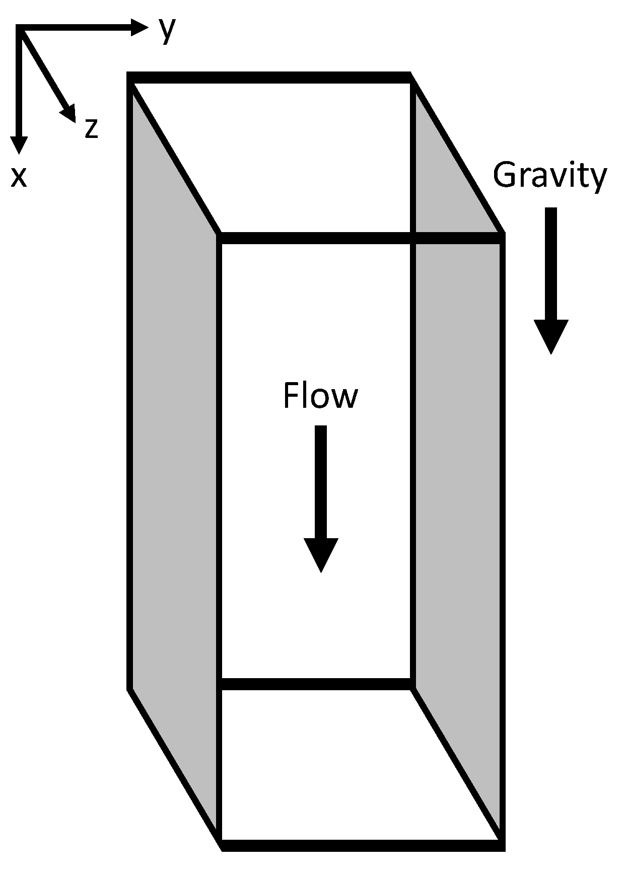
The setup investigated in this study, shown in Figure 2, is the so-called minimum channel [33], a vertical channel of size , and . The channel half-width H is taken to be unity, and x, y, z are the stream-wise, the wall normal and the span-wise direction, respectively. A downflow configuration is investigated, with the bubbles rising relative to the surrounding liquid. In main flow direction x as well as in the second homogeneous direction z, periodic boundary conditions are imposed, whereas the domain is bounded by no-slip walls in y-direction. The flow is driven downward by a constant volumetric flow rate , which is identical for all setups investigated in this study. The prescribed constant flow rate is the average steady-state flow rate of a single-phase channel flow simulation with a Newtonian fluid at a friction Reynolds number of , where is the average wall shear stress and is the kinematic viscosity of the liquid phase.
The density of the liquid phase is taken to be unity, and the density ratio of both phases is . For the Newtonian fluid ( and thus ), the dynamic viscosity ratio is specified as . This choice of the dynamic viscosity ratio is mainly made to avoid further complexity in addition to the variable viscosity of the liquid phase. The bulk Reynolds number, based on the total channel width , is .
While the three single-phase setups, one for each power-law index, are primarily considered for comparison purposes, the main interest lies in the six two-phase setups. These are investigated at a total gas volume fraction of 6%, which is achieved by including 72 bubbles with an identical initial diameter of . The simulation is initialized by inserting them into the velocity field of a fully developed single-phase channel flow using a uniformly distributed (x,y,z)-array of (6 × 3 × 4). To study the interplay of bubble deformability and power-law behavior of the liquid bulk, two different Eötvös numbers, , are considered. For the three setups with quasi-spherical bubbles, the surface tension coefficient is set in a way that the Eötvös number is . Furthermore, the gravitational acceleration g is chosen such that, for the two-phase setups with the Newtonian fluid, the Galilei number has a value of . This completes the set of material properties, which is selected to make the setup comparable to the pioneering study of Lu and Tryggvason [15]. Apart from the fact that the setups in their work are controlled by a constant pressure gradient instead of a constant volumetric flow rate, their case with the highest gas fraction is identical to one of the cases presented in this work ( and ). The higher Eötvös number of is achieved by decreasing the surface tension coefficient. Together with the other dimensionless numbers provided, this fully defines the investigated setup. For completeness, the values of the single parameters are given in Table A1 (Appendix A).
A joint analysis of and the bubble Reynolds number allows an estimation of the bubble deformation. The well-known Grace diagram [34], shown in Figure 3, divides the --space into different regimes representing a multitude of bubble shapes ranging from simple spheres to complex, skirted geometries. In this context, is defined as
For the characterization of the bubble dynamics, the phase-conditional averaging is limited to the bulk part of the channel . The wall boundary layers are excluded, as it is observed that the bubbles stay away from the walls (see Figure 6). To account for the variable viscosity of the non-Newtonian fluids and ensure consistency between the definitions of the relative velocity in stream-wise direction and the power-law based viscosity, the average apparent kinematic viscosity of the liquid phase is used in Equation (8). However, as will be shown later, the differences in are mainly due to the different relative velocities for this setup, while has a negligible influence on this parameter. The resulting values of are provided in Table 1, which gives an overview of all nine cases investigated in this study. All other conditions remaining identical, increases for the shear-thinning setup while the opposite effect occurs for the shear-thickening case. As just deviates slightly from the Newtonian case for and , only the two setups assuming are marked in Figure 3.
All setups investigated in this study are computed using a uniform grid of cells. Lu and Tryggvason [15] used computational points, uniformly spaced in the homogeneous directions, but unevenly spaced and clustered near the wall in the wall-normal direction. Moreover, it was reported that a finer grid of produced essentially the same statistical properties as the coarser grid. One of the setups simulated in this study (“tph10_loEo”) is identical to the setup investigated in [15], apart from the fact that the flow is driven downward by a constant volumetric flow rate instead of a constant pressure gradient. There are several reasons why a higher resolution of cells is convenient for the cases investigated here. First of all, as can be expected from Figure 3, the bubble deformations increase significantly for . A finer mesh more accurately captures bubbles exhibiting more complex shapes and oscillations, i.e., ellipsoidal or wobbling instead of quasi-spherical. In [17,35], a mesh of was used to simulate turbulent bubbly upflow for different Eötvös numbers, including . Moreover, the constant volumetric flow rate for the two-phase setups is taken to be that of the corresponding statistically converged single-phase flow at . As shown in [15], the volumetric flow rate decreases with increasing gas fraction when a constant pressure gradient is prescribed. Since the flow rate for the two-phase setups is determined using the initial conditions resulting from a single-phase setup, and kept constant, the observed flow rate is approximately 35% higher as the one reported in [15], which results from prescribing a constant pressure gradient. As a consequence, the bulk Reynolds number defined above also holds true for the two-phase setups in this study. Finally, as will be shown later, the wall-normal profile of the stream-wise velocity component close to the walls is steepest for the shear-thinning fluid, i.e., at the walls is, on average, observed to be the highest for and the lowest for . In order to accurately resolve the boundary layers at the walls in the shear-thinning case, it is therefore also advisable to increase the number of grid points from to . Using the latter resolution, the bubbles are resolved with approximately 20 cells in x- and z-directions, and 26 cells in the y-direction. The values of the first cell center at the wall, determined from with the apparent kinematic viscosity of the liquid phase, can be found in Table 1. For all investigated setups, the values are close to one. They are determined using the viscosity in the first cell at the wall. For this purpose, the viscosity fields have been averaged over the time as well as over the homogeneous directions x and z, see Section 4.1. The variable time step is controlled by setting for all setups.
4. Results and Discussion
This study aims to investigate both the effect the bubbles exert on the flow characteristics of the surrounding flow, as well as the influence the power-law behavior in the continuous phase has on the dispersed phase. To gain the respective insights, a number of quantities is evaluated after reaching the statistically steady state. Statistics are collected for a period corresponding to approximately 180 flow-through times () of the selected channel, starting after approximately 20 flow-through times () to exclude the initial transient. In this context, the reference time T is defined as , with the friction velocity of the initialization setup.
All statistics are computed using the definitions introduced in [18,19]. This allows for either collecting statistics for the whole domain, or for the liquid and the gas phase separately. The respective definitions are
where q is the quantity of interest, its fluctuation and denotes averaging over the time and the homogeneous directions x and z. Depending on which phase the statistics are conditioned on, c is either 1 (whole domain), f (only gas phase) or (only liquid phase). Unless indicated otherwise, the statistics are calculated for the whole domain (thus ) and averaged over the two halves of the channel. However, some statistics are not yet perfectly symmetric after the large number of flow-through times simulated. Averaging these statistics over the two channel halves could be misleading, since the lack of convergence can be confused with physical effects that are not really present. Therefore, these specific profiles have not been averaged with respect to the symmetry of the channel. Consequently, all wall-normal profiles, including the symmetric ones, are consistently shown for .
4.1. Average Wall Shear Stress and Viscosity Profiles
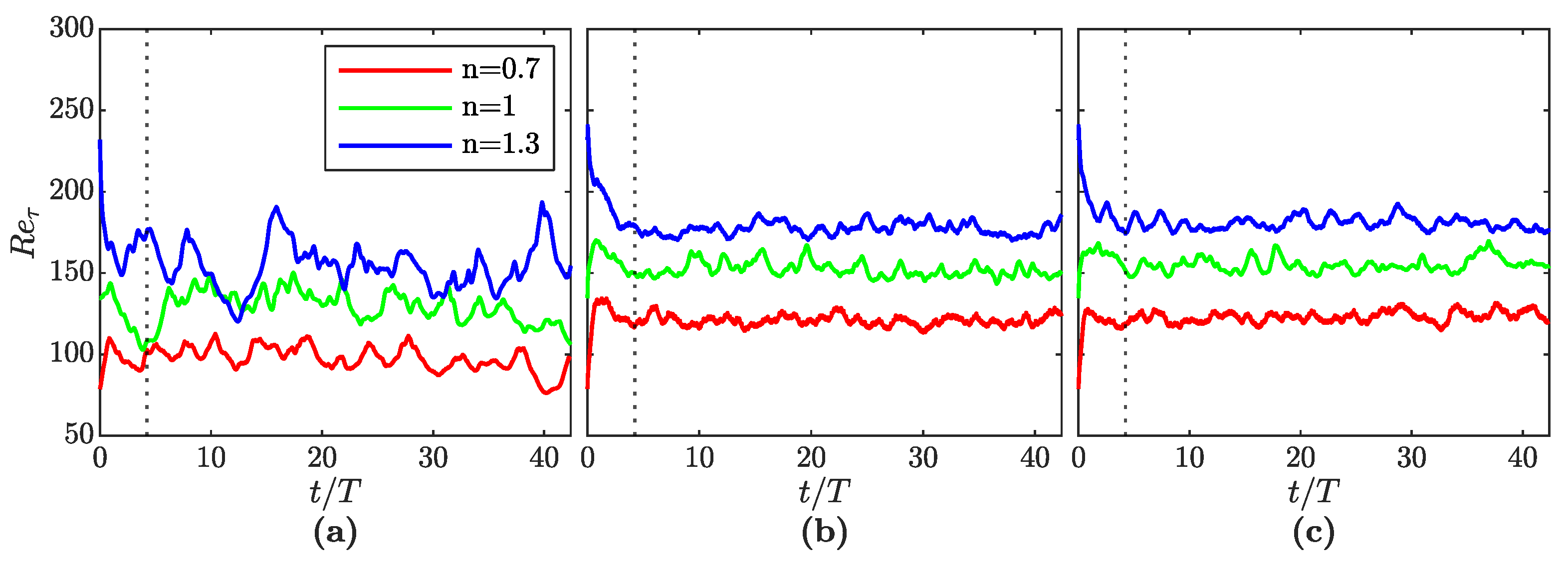
Typically, the convergence of bubble-laden channel flows towards a statistically steady state is measured using the average wall shear stress [15,19]. By normalizing it with , can be expressed in terms of the friction Reynolds number . Figure 4 shows , based on the wall-averaged shear stress , for all setups as a function of the time. The starting time of statistical averaging is illustrated by the dotted line at . As explained in Section 3.2, all cases are initialized from a single-phase channel flow of a Newtonian fluid controlled by a constant pressure gradient corresponding to . This value can be observed at for the three cases corresponding to . While of the single-phase case continues to fluctuate around this theoretical value when the flow control is changed to a constant volumetric flow rate, the presence of the dispersed gas fraction increases the average wall shear stress by approximately 20%. This effect was already reported in [19], where the authors attributed it to the stirring of the bubbles, which affects the near wall region above a certain gas fraction. The observed increase is 19.5% for and 21.7% for . Although the time-averaged wall shear stress of the single-phase setup for deviates from the theoretical value by less than 2%, the respective fluctuations are found to be stronger compared to the two-phase cases. The presence of the bubbles has a clearly visible dampening effect on the fluctuations of , irrespective of the power-law index.
As Figure 4 shows, the wall shear stress increases when the continuous liquid phase exhibits shear-thickening behavior (), while the opposite effect can be observed for the shear-thinning scenario (). This behavior is dominated by the viscosity values close to the walls. Due to the high shear rates in the near-wall region, the viscosity of the shear-thickening fluid exceeds the viscosity of the Newtonian fluid, while the viscosity of the shear-thinning fluid follows an opposite trend, see Figure 5. Although the mean velocity gradient at the wall is slightly higher (lower) for the shear-thinning (shear-thickening) fluid (see Figure 7), the wall shear stress still reveals the lowest (highest) values due to the viscosity behavior. The findings observed for the Newtonian fluid, i.e., smoother curves of with fluctuations around an increased average value for two-phase setups, also hold true for the non-Newtonian fluids.
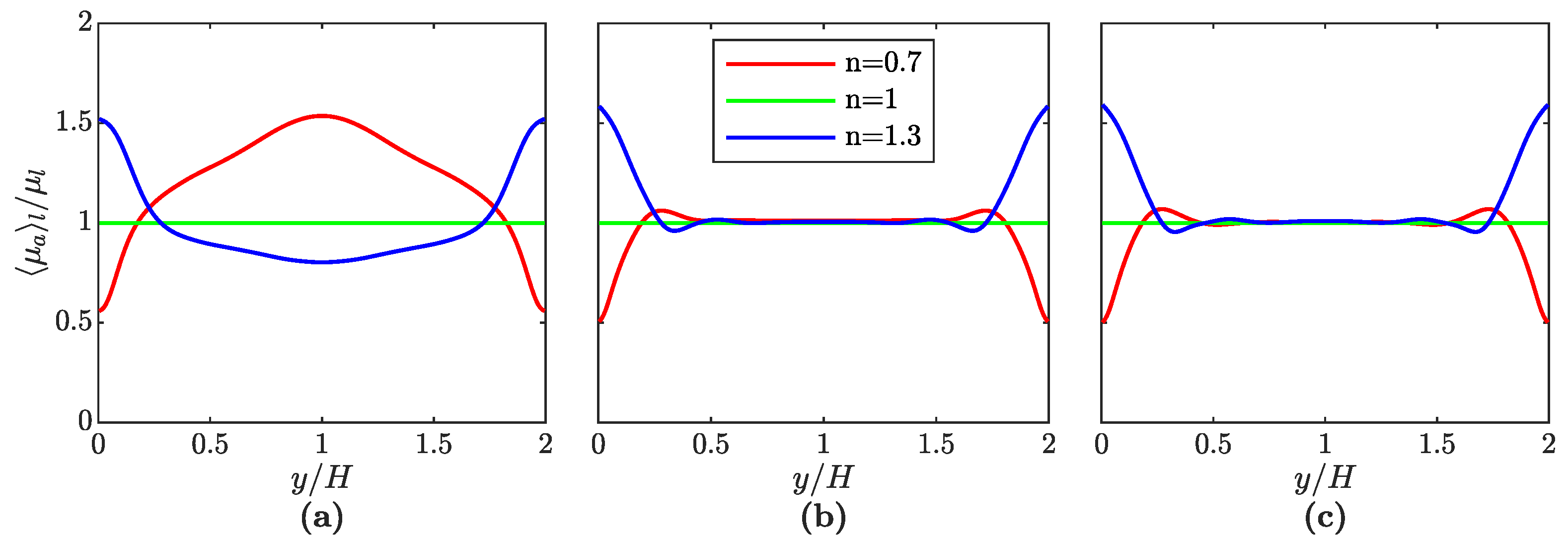
Since the three cases in each setup category, i.e., single-phase or two-phase with either quasi-spherical or deformable bubbles, are identical apart from the different power-law indexes, it is expedient to initially investigate the viscosity statistics of each case. The viscosity values do not only explain the above-mentioned observations regarding the average wall shear stress, but they are also responsible for all other differences occurring in the results of one setup category. Figure 5 shows the average apparent dynamic viscosity of the liquid phase , normalized with the viscosity for , as a function of the wall-normal coordinate y.
For the single-phase cases with a non-Newtonian continuous phase, the dynamic liquid viscosity obeys a monotonic trend from the wall to channel center. As the shear rate is high close to the walls and low in the channel center, the shear-thinning fluid produces the minimum viscosity at the walls, while the maximum can be found in the center. The opposite behavior can be observed for the shear-thickening fluid. While the profiles for the two-phase cases are relatively similar to those of the respective single-phase setups close to the walls, they clearly show the range where the bubbles are present, which spans from to (see Section 4.2). Due to the bubbles accumulating in this part of the domain, there are elevated local velocity differences causing the shear rate to exceed the values from the single-phase setups. As a consequence, the viscosity increases (decreases) for the shear-thickening (shear-thinning) fluid and the profiles for different power-law indexes are very close to each other in the section around the channel center. Moreover, due to the homogeneous bubbly flow in the core part of the channel (see Figures 7 and 9), , the average shear rate (see Section 2) as well as the average apparent viscosity are almost independent of y and constant in this region. It is also interesting to note that the Eötvös-number, and therefore the bubble deformability, seem to have a negligible influence on the viscosity profiles. Table 2 provides the normalized average viscosities of the liquid phase, which result from averaging over all spatial directions and over the time.
When investigating the average viscosity profiles for the bubble-laden flows, the quasi-identical values in the channel center lead to the question of whether there is some underlying physical cause for this behavior. As discussed in Section 2, the apparent liquid viscosity for the power-law fluids is determined as . In order to observe identical average liquid viscosities across all investigated power-law indexes in the channel center, the average shear rate in this region would have to be equal to one. Since there is no obvious reason why this should generally be the case, it is assumed that this is just a characteristic of this specific setup and not a general observation. To verify this, a set of additional simulations has been performed at an increased void fraction of 10%. Indeed, the results support this assumption. For 120 instead of 72 bubbles, the average shear rate in the channel center increases further. This leads to a situation where, in contrast to the results illustrated in Figure 5, the viscosity profiles, including the peaks, for the shear-thinning fluid fall below the constant viscosity of the Newtonian fluid for all values of y. The same effect, yet in the opposite direction, holds for the shear-thickening fluid: the minima are still larger than . While, in principle, the shape of the profiles remains very similar, this shows that increased shear rates in the channel center due to higher gas fractions shift the viscosity profiles in the center towards the values at the wall. The single-phase setups in Figure 5 demonstrate this observation for the opposite extreme case. Another change to the setup that should, in principle, evoke similar consequences on the viscosity profiles would be to choose the power-law indexes for the shear-thinning and thickening fluid to be further away from 1. However, additionally verifying this assumption was beyond the scope of this work, as, with regard to Figure 5, it should only be clarified that the quasi-identical values in the channel center are indeed a characteristic of this specific setup and not a general observation.
4.2. First- and Second-Order Fluid Statistics
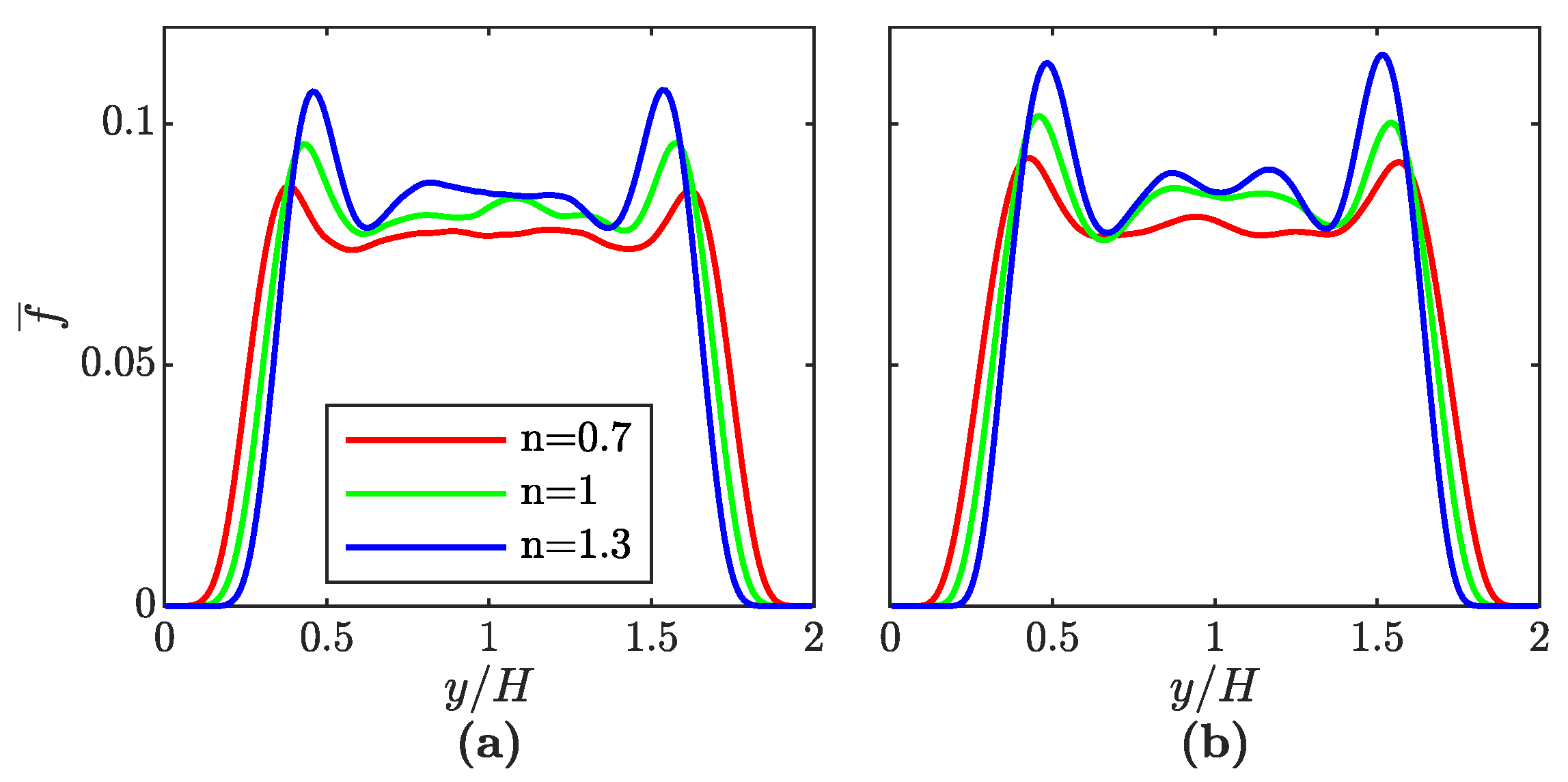
As was already reported in earlier studies investigating bubble-laden downflow channels [15,16,19], the bubbles show a clear tendency to accumulate in the channel center, see Figure 6. According to Lu and Tryggvason [15], this can be explained by the lift force acting on the bubbles. While all profiles exhibit the characteristics known from earlier studies, namely a relatively constant distribution in the channel center together with peaks in the transition to the bubble-free regions near the walls, there are clear tendencies arising for the shear-thinning and the shear-thickening fluid. It is important to note that the profiles shown in Figure 6 have not been averaged over the two channel halves. As can be recognized, the profiles are not perfectly symmetric. This indicates that the volume fraction field tends to converge slower than the other statistics provided in the following sections, which achieved a high degree of symmetry. Nevertheless, the profiles illustrated in Figure 6 are very similar to what is known from literature, with only one exception: the distribution is less uniform in the channel center. In order to make sure that this behavior only occurs due to a lack of convergence, identical setups have been simulated for a void fraction of 10%. As was observed in [19], statistics collected for dense cases tend to converge faster than those gathered at dilute gas fractions. For the increased gas fraction, it was possible to observe profiles that exhibit a high degree of symmetry together with flat profiles in the bubble-rich core. Consequently, it can be estimated that the profiles presented in Figure 6 would only flatten in the center for significantly longer simulation periods, while otherwise retaining their characteristics. Since the gathered statistics have already been computed over 180 flow-through times it is likely that, in order to reach void fraction profiles exhibiting perfect symmetry, a significantly longer simulation is required. As this study primarily aims to show tendencies arising for a non-Newtonian continuous liquid phase, it was decided to not continue the simulations.
When comparing the void fraction profiles for the cases with to the profiles with a non-Newtonian liquid phase, clear tendencies can be observed. First of all, the bubble-free zone near the walls is wider for the shear-thickening and narrower for the shear-thinning setup. As a consequence, the profiles for are shifted towards the channel center. Since the overall gas fraction is identical for all cases, this results in a stronger accumulation of bubbles in the core of the channel. Therefore, both the peaks in the transition between core and walls as well as the plateau-like section in the center are shifted to higher values. The opposite holds for , where the bubbles are distributed more uniformly along the wall-normal direction. The shear lift force occurs due to the mean flow gradient near the wall. As the boundary layer becomes thinner (thicker) for shear-thinning (shear-thickening) fluids (see Figure 7), the bubbles move closer to (stay away further from) the wall compared to the Newtonian case. However, the peaks do not only increase for higher values of n. A comparison of the profiles for and reveals that, independent of the power-law index, the profiles are also shifted towards the channel center for increased . This impacts the peaks in the same way as described for increased values of n.
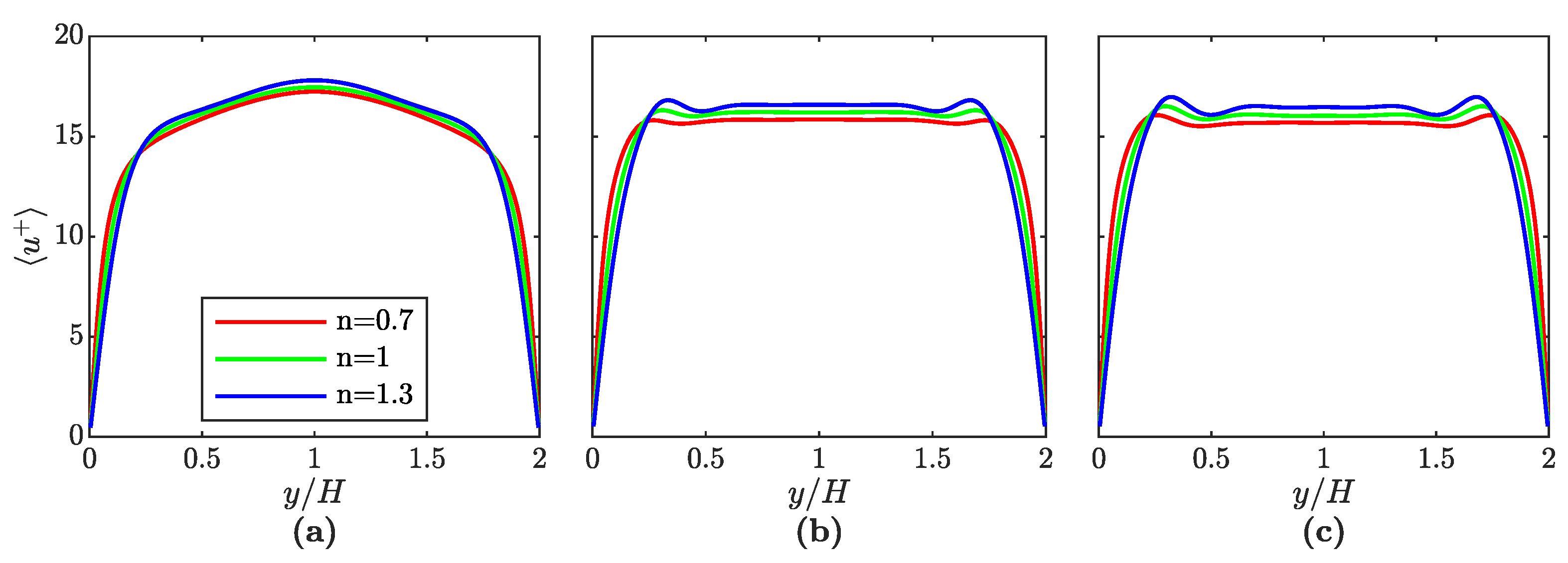
The profiles for the average stream-wise velocity , normalized with the friction velocity to yield , are shown in Figure 7. Since the actual friction velocity is different for each of the nine setups (see Figure 4), the value is taken from the initialization setup. The theoretical value for the respective case is provided in [15]. All profiles are similar to the ones shown in the literature, i.e., the single-phase setups show a monotonous increase towards their maximum value in the channel center, while the two-phase setups exhibit an almost uniform profile in the region of the bubble-rich core. In principle, the effect of increasing or decreasing n is the same as shown for the void fraction profiles in Figure 6. Once again, the profiles for the shear-thickening setups are shifted towards the channel core and, due to the constant volumetric flow rate, exhibit higher average velocities there. On the other hand, the profiles for the cases considering the shear-thinning fluid are wider and reach lower maximum flow velocities. The thickness of the wall boundary layer increases with n. This observation is consistent with the viscosity profiles illustrated in Figure 5, which demonstrate that the viscosity in the near-wall region is high for the shear-thickening fluid and low for the shear-thinning fluid. It is also interesting to note that a plateau-like section is formed in the middle of the two-phase velocity profiles, between the locations of the volume fraction peaks. In this regard, the profiles resemble the one shown in [18], although the plateaus are more pronounced in the present study, especially for . This can be partly attributed to the fact that, instead of excluding the velocities of the gas phase, the velocities of both phases are taken into consideration here. Since the bubbles rise relative to the continuous liquid phase, including the gas-phase velocity would result in lower flow velocities in the bubble-rich channel core. For the two-phase setups, the velocity profiles exhibit only minor differences between and . As can be seen, the peaks and plateau-like sections of the profiles are slightly more pronounced for the higher Eötvös number.
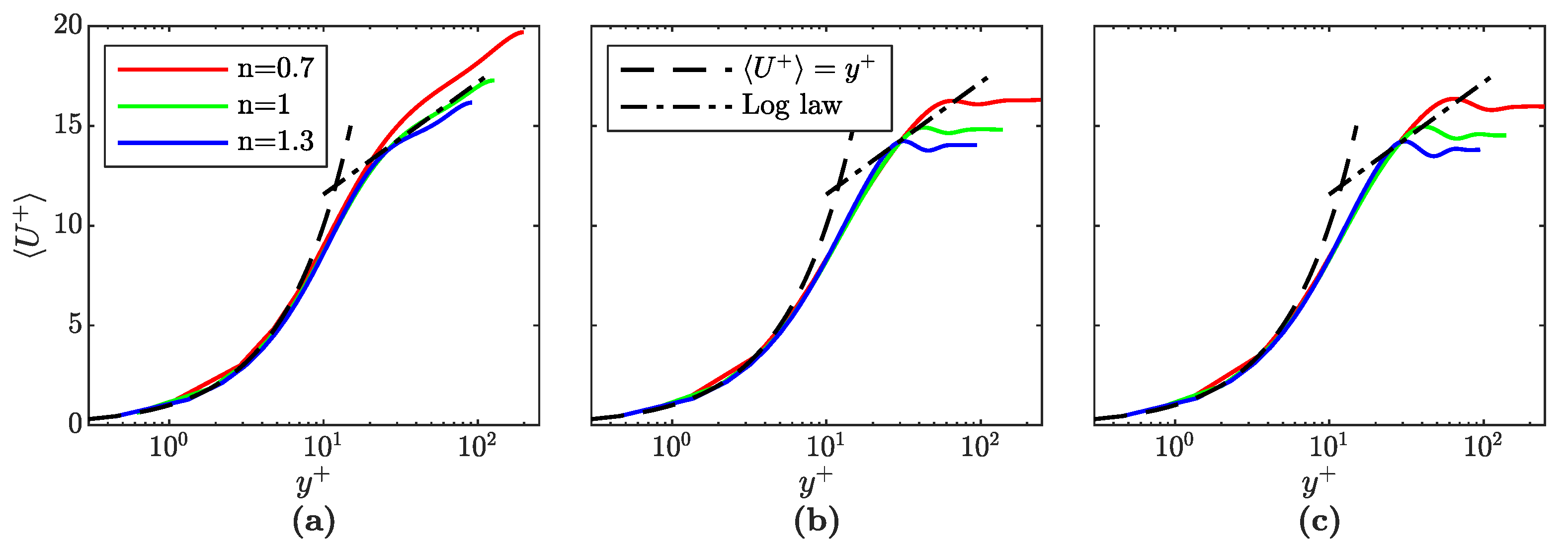
Figure 8 shows a semilogarithmic plot of the stream-wise velocity , normalized by the friction velocity to yield the dimensionless velocity , over the the dimensionless wall distance . It is important to note that, in this context, is determined using the actual value of the wall shear stress for each setup (see Figure 4) instead of the theoretical value corresponding to the initialization setup, which was used for the profiles in Figure 7. This is indicated by using instead of in the following. For the calculation of the friction velocity, is averaged over the same time span as all other statistics. The dimensionless wall distance is defined as . However, the kinematic viscosity is not constant for the non-Newtonian fluids. Since the aim is to investigate the flow behavior close to the wall, the viscosity values for the power-law fluids are taken from the first cells at the wall, i.e., corresponds to the average apparent viscosity values of the liquid phase at and , see profiles shown in Figure 5. Since the near-wall region is free of bubbles, the kinematic viscosity of the gas phase does not play a role for the determination of . The resulting profiles are compared to the theoretical approximations suggested in the literature. For the viscous sublayer (), the predicted behavior is . In the logarithmic layer (), the figure compares the normalized velocity to the logarithmic “law of the wall”, or “log law”, which is defined as . Here, is the von Karman constant and B is taken to be 5.95 [15].
As Figure 8 shows, all nine profiles agree very well with in the viscous sublayer. While the velocity of the single-phase flow at also matches the “log law” very accurately, the profiles are shifted to higher values for the shear-thinning and to lower values for the shear-thickening fluid. Due to the absence of bubbles close to the walls, the two-phase profiles are relatively similar to those of the single-phase flow up to the position where the velocity peaks are formed. At larger distances from the wall, the stream-wise velocity profiles for the bubble-laden flows increasingly deviate and flatten towards the bubble-rich core region. As has also been reported in [15,18], the thickness of the wall boundary layer is reduced due to the presence of the bubbles and the formation of a logarithmic layer can therefore not be observed.
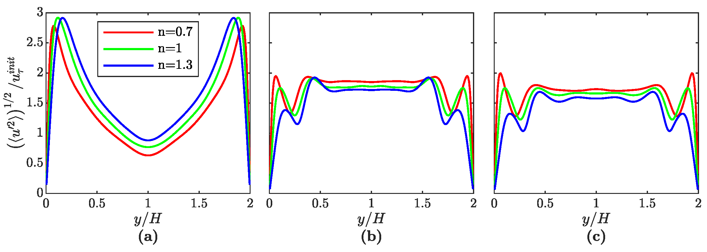
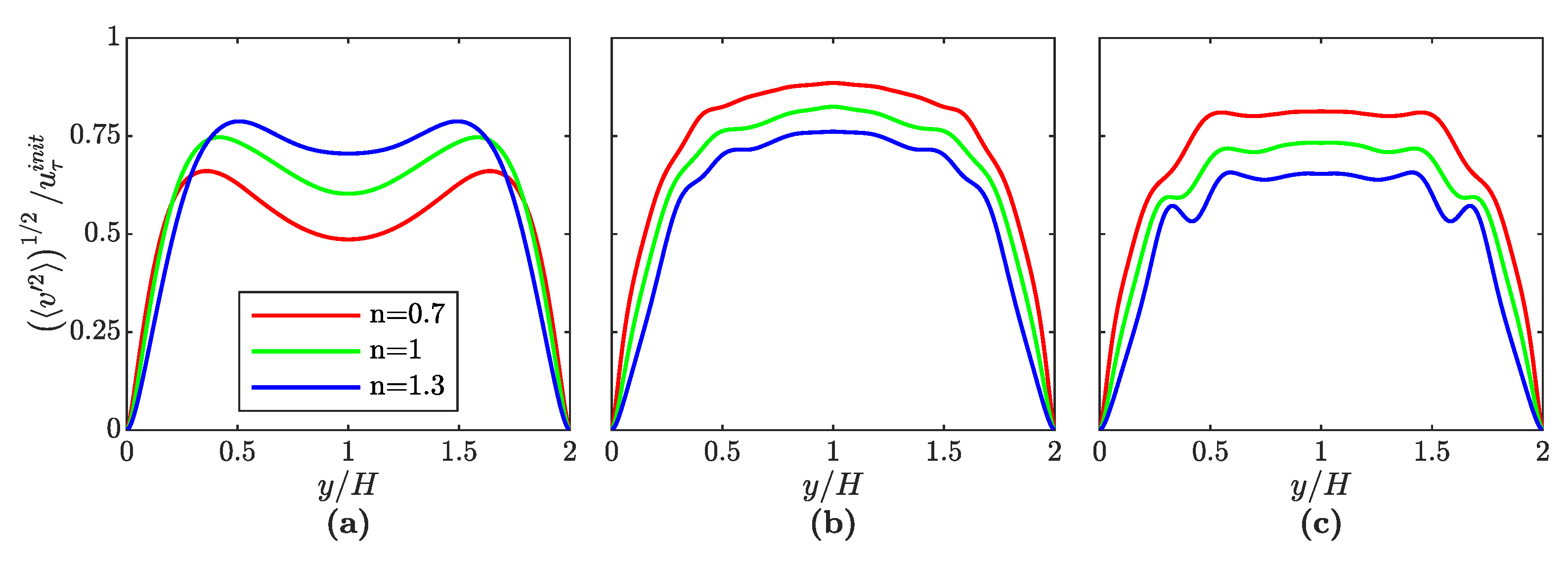
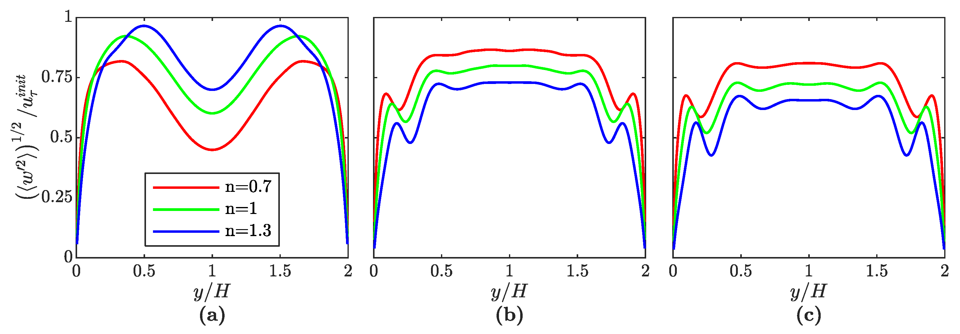
Figure 9, Figure 10 and Figure 11 show the root mean square of the stream-wise, the wall-normal and the span-wise velocity fluctuations, normalized by the friction velocity of the initialization case . Overall, the fluctuations for strongly resemble the profiles reported in the literature [15,18,19]. The introduction of a dispersed phase at a significant void fraction leads to clear deviations of all profiles from their single-phase counterparts. The stream-wise velocity fluctuations for the single-phase setups, illustrated in Figure 9, reach their maximum close to the wall, followed by a decrease towards the channel center. Independent of the power-law index, the opposite behavior can be observed for the two-phase setups. Figure 9 shows that, although the first peaks of the bubble-laden flows are located at the same values of y, they are significantly lower. This indicates a strong turbulent intensity reduction in the near-wall region. As discussed in [18], the reason for this observation might be that, due to their lower velocity compared to the liquid bulk, the bubbles act as obstacles and intermit the otherwise present turbulence structures. On the other hand, compared to the single-phase setups, the two-phase flows reveal increasing fluctuations of the stream-wise velocity component in the channel core, which are generated by the high number of bubbles present in this region [15]. As can be seen, the stream-wise fluctuations are virtually independent of y in the bubble-rich core, where the bubbles are distributed evenly (see Figure 6).
The latter observation also holds true for the velocity fluctuations in the other spatial directions. While the two-phase profiles for the wall-normal fluctuations, illustrated in Figure 10, show a slight increase from the locations of the void fraction peaks towards the channel center for , the profiles for and those for the span-wise velocity fluctuations, shown in Figure 11, are relatively independent of y in the middle section. As shown in [18,19], all fluctuation profiles generally tend to flatten completely in the core region, if the void fraction is increased to values of 10% or more.
In the next step, the influence of the power-law index on the velocity fluctuations is investigated. For the single-phase setups, the difference in the velocity fluctuations close to the wall is insignificant. However, this changes towards the channel center, where the highest fluctuations can be observed for , while the single-phase flow at reveals the lowest fluctuations. These findings hold true for the stream-wise, the wall-normal and the span-wise direction. The observed profiles can be explained by the differences in the shear rate. For the single-phase channel, the shear rates are high in the near-wall region and low in the channel center. As a consequence, the shear-thinning (shear-thickening) fluid exhibits a low (high) dynamic viscosity close to the wall and a high (low) dynamic viscosity in the channel center, see Figure 5. As the strength of the fluctuations is expected to increase with decreasing dynamic viscosity, this explains the trends observed for the single-phase setups. However, this effect is partially countered by the increasing gradients close to the wall for decreasing power-law indexes, such that the peaks of the stream-wise velocity fluctuations remain more or less comparable for all cases.
As shown in Figure 9, Figure 10 and Figure 11, the two-phase profiles for the fluctuations of all three velocity components reveal remarkable differences compared to their single-phase counterparts. It is especially interesting to note that the order regarding the fluctuation strength is reversed in the bubble-rich core once a significant amount of bubbles is present. The two-phase setups with a shear-thinning continuous phase not only exhibit the strongest fluctuations close to the walls, but also in the bubble-rich core and for almost all values of in the transition between these regions. While the three profiles of the stream-wise fluctuations overlap marginally for some small sections of , the wall-normal and span-wise velocity fluctuations for are higher than those for independent of the wall-normal coordinate. The profiles for are generally located between those of the non-Newtonian fluids apart from small overlaps on each side. The introduction of a significant number of bubbles leads to higher local velocity differences and increasing shear rates in the bubble-rich core. As a result, the apparent viscosity of the shear-thinning fluid decreases compared to the single-phase setup, while the opposite effect holds for the shear-thickening fluid. However, as shown in Figure 5, the profiles of the average apparent viscosities are quasi identical in the channel core and therefore cannot fully explain the results observed for the fluctuations. The findings can, however, be reasoned by the different viscosities in the vicinity of the phase interface, where the velocity fluctuations are generated. For the single-phase setups, the fluctuations for -positions very close to the walls are strongest (weakest) for (), as the shear rate is high close to the walls. As an additional analysis revealed, high shear rates occur in the vicinity of the phase interface as well. This can also be recognized in Figure 15, where strong velocity gradients are clearly visible around the bubbles. As a consequence, the apparent liquid viscosity for the shear-thinning (shear-thickening) fluid is significantly lower (higher) than the one of the Newtonian fluid in the vicinity of the phase interface. Although, partly due to the migration of the bubbles, this effect is not visible in the averaged profiles (see Figure 5), it is responsible for the stronger (weaker) velocity fluctuations (compared to ) observed for the shear-thinning (shear-thickening) fluid in the core region. Moreover, the fluctuations in the core occur mainly due to the vortex shedding in the bubble wake and the velocity differences between the bubbles and the surrounding liquid. As discussed in Section 3.2, all other conditions remaining identical, the relative velocity of the bubbles, and therefore also the bubble Reynolds number, increases with decreasing power-law index. This also explains the trends observed for the velocity fluctuations in the channel core.
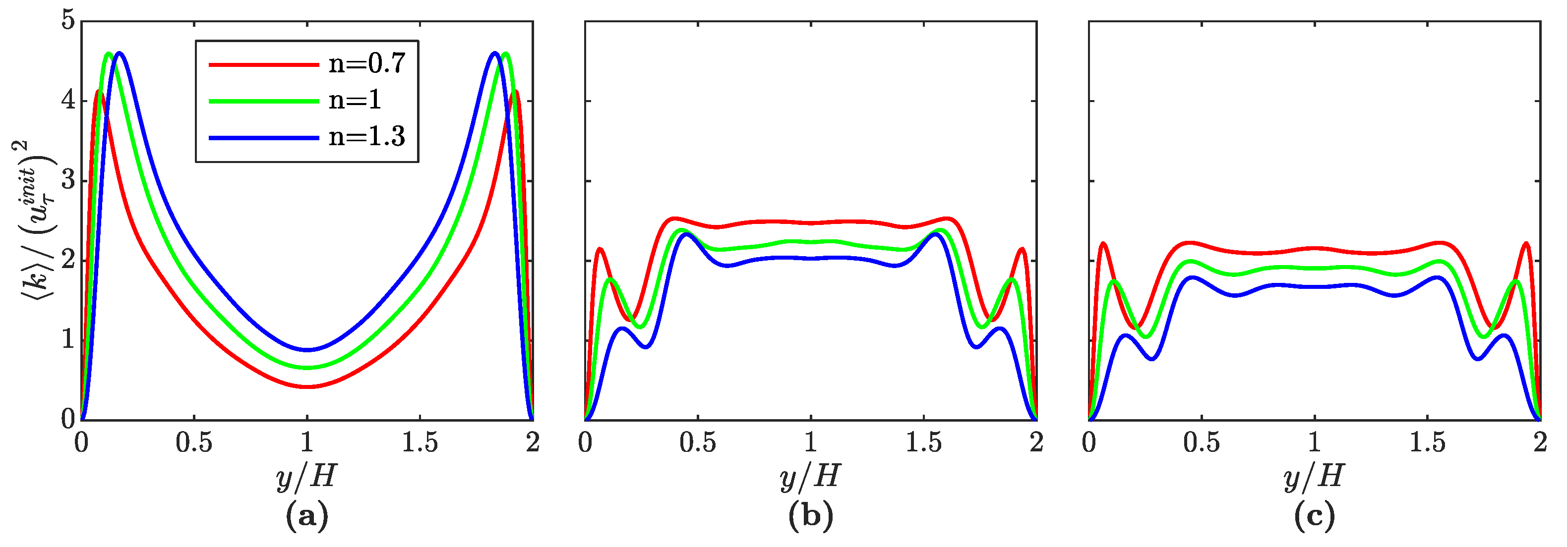
Compared to the strong influence of the power-law index, the changes observed when increasing the Eötvös number from 0.3125 to 3.75 are relatively small. For the stream-wise velocity fluctuations (see Figure 9), the peaks in the near-wall region are slightly more pronounced. Moreover, a minimal displacement of the profiles away from each other in the transition to the bubble-rich core can be observed. The same applies to the span-wise (Figure 11) and the wall-normal (Figure 10) fluctuations. For the latter, additionally leads to a flattening in the center. However, it is interesting to note that the fluctuation of all velocity components is generally stronger for the lower Eötvös number. Although the differences are small when comparing the velocity fluctuation profiles, this effect is clearly visible when investigating the turbulent kinetic energy k, see Figure 13. Further analysis regarding this observation, as well as the impact on the dissipation rate , can be found in Section 4.3.
4.3. Dissipation Rates
In this section, the dissipation rate of the turbulent kinetic energy is investigated. It can be defined as
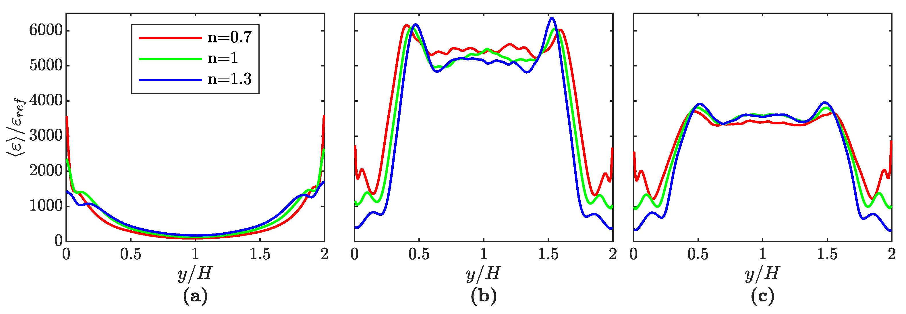
with the apparent kinematic viscosity and the velocity fluctuations . The averaging over time and the homogeneous directions are consistent with the procedure used for the first and second order fluid statistics (see Section 4.2). The apparent kinematic viscosity is . Figure 12 shows the dissipation rate, normalized with the reference value for and evaluated without phase-dependent conditioning, as a function of the wall-normal coordinate. The profiles have not been averaged over the two channel halves.
For the three single-phase setups, the dissipation rate reaches its maximum at the walls, while the minimum is located in the channel center. In the near-wall region, the dissipation rate decreases with increasing power-law index. However, the order reverses at a distance of approximately from the walls. This behavior can be deduced from the fluctuations of the three velocity components (see Figure 9, Figure 10 and Figure 11), where similar trends can be observed. It is worth noting that viscosity plays a role as well, but the velocity fluctuation gradients have a quadratic contribution to the dissipation rate. The two-phase setups are dominated by the presence of the bubbles in the core of the channel. Since (see Section 3.2), the kinematic viscosity of the gas phase is significantly higher than the apparent kinematic viscosity of the liquid phase. For the Newtonian fluid, is 10. As a consequence, there is a direct relation between the void fraction (see Figure 6) and the dissipation rate profiles (see Figure 12) and the corresponding profiles exhibit a very similar shape. The two-phase profiles do not only deviate from their single-phase counterparts in the center of the channel, but also close to the walls. This reflects the significant deviations of the two-phase velocity fluctuation profiles from their single-phase counterparts, occurring for practically all values of y (see Figure 9, Figure 10 and Figure 11).
The Eötvös number has a negligible influence on the dissipation rate in the near-wall region. In the channel center, however, the dissipation rates for are significantly higher than those for . This can be reasoned by the behavior of the average turbulent kinetic energy , illustrated in Figure 13, and the integral turbulent length scale ℓ. The relation between the dissipation rate and the turbulent kinetic energy is . As shown, the profiles of k for the setups at are shifted to higher values compared to their counterparts at . As the difference in k is less pronounced than the difference in , the behavior of ℓ must also be considered. As will also be discussed in Section 4.4, the bubbles are deformed to an ellipsoidal shape for , while they remain quasi-spherical for . For spherical bubbles, it is possible to assume . For the ellipsoidal bubbles, on the other hand, the integral length scale approximately corresponds to the lateral expansion of the ellipsoid perpendicular to the main flow direction. Therefore, it is reasonable to assume that for the setups at . Combined, the differences in k and ℓ explain the observations for the dissipation rate. It is, however, not trivial to identify the reason for the dependency of k on the the bubble deformability. As discussed in Section 3.2, the bubble Reynolds numbers are higher for the setups at (see Table 1), which is indicative of stronger velocity fluctuations in the bubble wake. These higher values of are caused by higher stream-wise velocity differences between the bubbles and the liquid phase. Nearly spherical bubbles encounter less resistance while rising through the liquid, which allows them to rise faster than the deformable bubbles. Moreover, it is worth noting that there is a constant interplay between interfacial surface energy and turbulent kinetic energy, as discussed by Dodd and Ferrante [36].
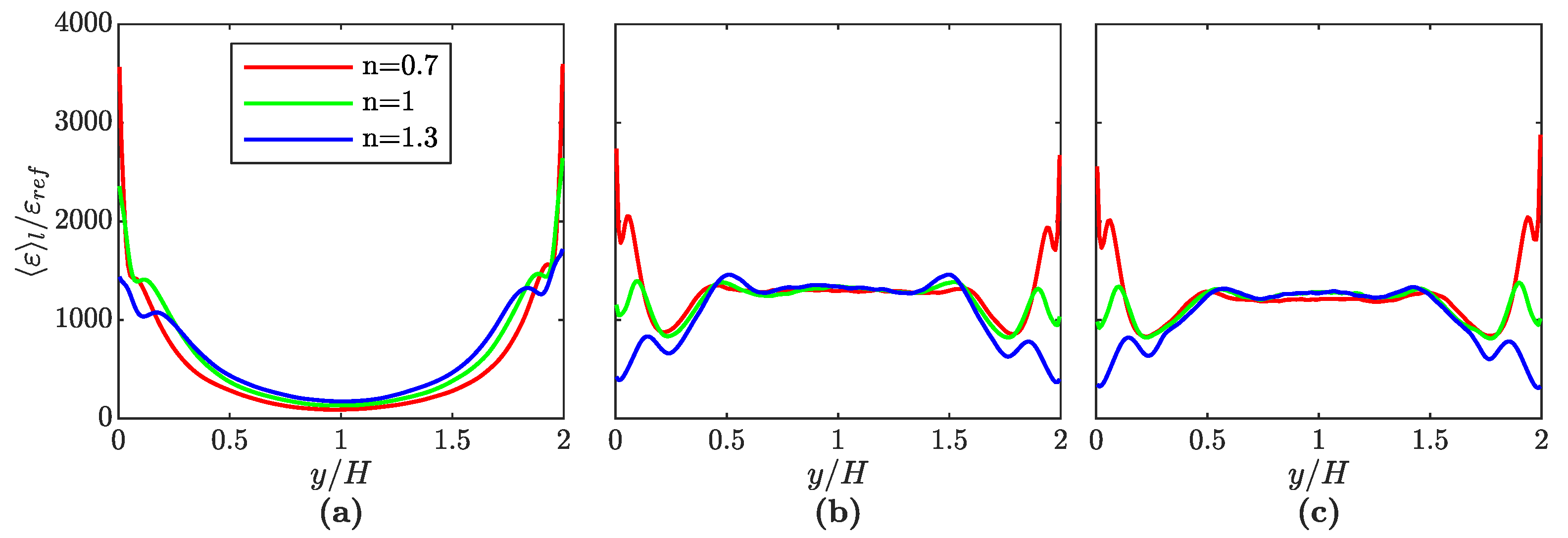
In order to exclude the effect the high kinematic viscosity of the bubbles has on the dissipation rate, Figure 14 provides the average normalized dissipation rate conditioned on the liquid phase . The profiles have not been averaged over the two channel halves. The single-phase profiles, given for comparison, are identical to those shown in Figure 12. As observed for , the presence of the bubbles completely changes the profiles for all power-law indexes. In the near-wall region, the two-phase cases for and exhibit significantly lower dissipation rates compared to the single-phase flow. For , this observation only holds true directly at the wall. At larger distances from the wall and especially in the core of the channel, the bubbles significantly increase the liquid phase dissipation rate irrespective of the power-law index. For , the dissipation rate in the channel center is approximately as high as its peak value in the near-wall region. It is especially interesting to note that, for the shear-thickening fluid, the presence of the bubbles completely reverses the trends resulting for the single-phase setups. The minimum dissipation rate can be observed at the walls. The highest dissipation rates occur from to in the form of a plateau-like section. This behavior can partly be attributed to the apparent viscosity in the channel core, which, compared to the corresponding single-phase flow, reaches higher values for the bubbly flow setups at (see Figure 5). Moreover, we refer to the relation between k and explained above. Compared to the single-phase flows, including the bubbles significantly lowers the values of k close to the walls (see Figure 13), in particular for . Together with the higher turbulent kinetic energy in the channel core, which can be observed irrespective of n, this explains the two-phase profiles of the dissipation rate at , shown in Figure 14.
4.4. Bubble Deformation
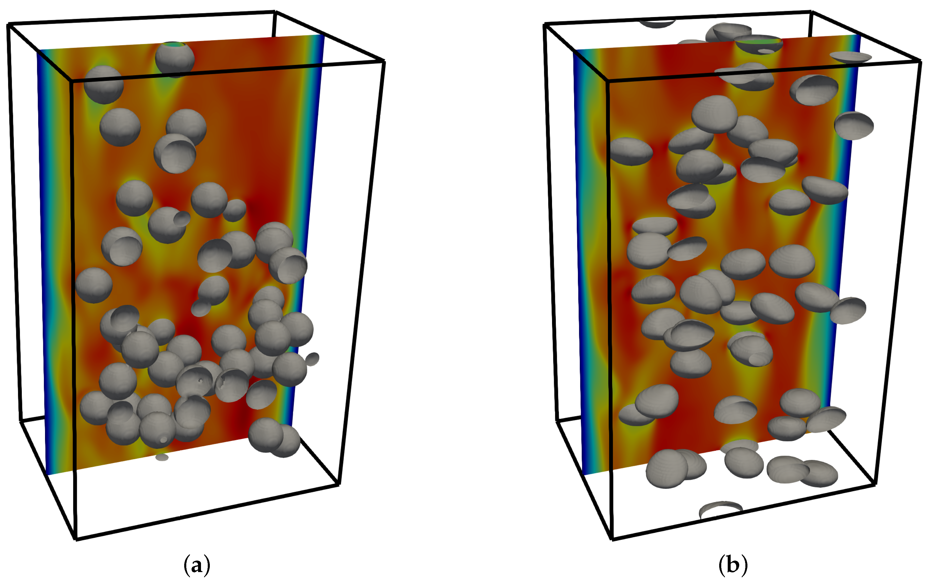
As explained in Section 3.2, the dynamic bubble behavior can be estimated from the Eötvös number and the bubble Reynolds number using the Grace diagram, see Figure 3. A straightforward way to investigate the bubble shapes occurring for the different setups is to visualize the isocontours corresponding to , i.e., the interface between gas and liquid phase. Snapshots for the bubbly-flow cases with a Newtonian fluid in the continuous phase are shown in Figure 15. Since there are hardly any visible differences for the non-Newtonian fluids, the respective plots are omitted. The isosurfaces confirm the prediction of the Grace diagram. As expected, the bubbles are quasi-spherical for . However, when is increased to , the bubbles are wobbling and assume an ellipsoidal shape.
While this allows a first qualitative assessment of the bubble deformations, snapshots at a single time step do not yield further insights into the transient deformation behavior as well as the effects of different power-law indexes. In order to provide a meaningful quantitative measure for the bubble deformation, it is expedient to analyze the temporal behavior of the interface area for the single bubbles. For this purpose, the interface area of a bubble b is numerically approximated as the volume integral of , which can be interpreted as the surface density, over all cells belonging to the bubble’s individual VOF marker field. It is necessary to perform this analysis for all bubbles separately. Otherwise, the oscillations of the individual bubbles would annihilate each other due to the different instantaneous deformation behavior. In the following, denotes the the surface area of bubble b at the time t, normalized by the surface area of a sphere of the same volume V. The time-averaged, normalized surface area is given as
with the start and end times and for gathering statistics. The fluctuation of the normalized surface area around this value is then evaluated using the root mean square:
Finally, the time-averaged, normalized surface areas and the fluctuations are averaged over all 72 bubbles. The results are presented in Table 3.
Table 3 shows that the normalized surface area averaged over time and all bubbles grows by 6.40% for the shear-thinning, by 5.84% for the Newtonian and by 5.08% for the shear-thickening fluid when the Eötvös number is increased from 0.3125 to 3.75. Moreover, it is clearly visible that the bubbles are not only deformed to ellipsoids for . Measured in terms of their surface area fluctuations, they are also subject to much stronger oscillations. Compared to , the values of increase by a factor of 40.42 for , by a factor of 48.25 for and by a factor of 55.73 for . Finally, and show clear tendencies across the investigated power-law indexes. Both quantities increase for decreasing values of n. This behavior can be explained by the values of the bubble Reynolds number given in Table 1, which also increase with decreasing power-law index. As shown in the Grace diagram (see Figure 3), the bubble deformability is governed by the combination of and . At identical , higher values of are indicative of stronger deformations and oscillations. It was found that the differences in the values of are almost exclusively caused by the different relative stream-wise velocities of both phases, see Equation (8). On the other hand, the apparent liquid dynamic viscosities in the center part of the channel () seem to only have a negligible influence, as can be seen in Figure 5.
5. Conclusions
In this paper, turbulent bubble-laden channel flow of power-law fluids at a bulk Reynolds number equal to 3790 was studied by means of Direct Numerical Simulation (DNS). The power-law index n was varied between 0.7 (shear-thinning), 1 (Newtonian) and 1.3 (shear-thickening). The downflow channel was loaded with 72 either quasi-spherical () or ellipsoidal/wobbling () bubbles, which resulted in a total gas fraction of 6%. In addition, corresponding single-phase setups were investigated for comparison. The results demonstrate the intricate interaction of non-Newtonian and bubbly flows:
For the single-phase flow at (), the apparent viscosity of the liquid phase reaches its maximum (minimum) directly in the center of the channel, due to the low shear rates away from the walls. It was observed that the presence of the dispersed phase significantly increases the shear rate in the channel core, where the bubbles accumulate. Therefore, compared to the single-phase flow at identical power-law index, the apparent viscosity of the liquid phase in this region decreases (increases) for the shear-thinning (shear-thickening) fluid. In comparison to the single-phase flow, a flattening of the viscosity profiles, irrespective of , can be observed in the channel core due to the homogeneous bubbly flow in this region. In the bubble-free near-wall region, the behavior of the viscosity remains nearly unchanged when including the bubbles. The bubble-free zone near the walls is wider for , which leads to a stronger accumulation of bubbles in the core. The opposite effect is observed for , i.e., the bubbles, on average, move closer to the walls. The profiles of the average stream-wise velocity demonstrate that the thickness of the wall boundary layer increases with n. In the near-wall region, the shear-thickening fluid exhibits the lowest flow velocities, while the highest velocities are observed for the shear-thinning fluid. Since the constant volumetric flow rate is identical for all setups, this order reverses in the core of the channel. As reported in other studies, the velocity profiles of the two-phase setups flatten and form a plateau-like section in the bubble-rich ore.
The presence of the bubbles significantly changes the fluctuation profiles of all three velocity components. For the single-phase flows, the strength of the fluctuations in the channel core increases with n. For the two-phase setups, this order is reversed. It is interesting to note that, overall, the velocity fluctuations and therefore the turbulent kinetic energy for are higher compared to . For the less deformed bubbles at , this difference, together with the lower integral turbulent length scale due to the quasi-spherical bubble shape, leads to a higher turbulence dissipation rate in the channel core. It was additionally shown that, compared to the single-phase setups, the presence of the dispersed phase significantly increases the dissipation rate in the region where the bubbles accumulate. For , the trend observed for the single-phase setup reverses entirely, i.e., the dissipation rate of the liquid phase reaches its maximum in the bubble-rich core, while the minimum was found to be located directly at the walls.
Finally, an analysis of the mean value and the fluctuation of the bubble surface areas revealed that, irrespective of the Eötvös number, the average deformation and oscillation strength increases with decreasing power-law index. As expected, the average deformation and oscillation strength were observed to be more pronounced for .
The present analysis has been carried out with the power-law model. To take into account additional effects present in real-world non-Newtonian fluids, more sophisticated models, such as the Bird–Carreau or Cross-Power-Law model, can be considered for further investigations.
Author Contributions
Conceptualization, M.K. and J.H.; formal analysis, F.B. and E.T.; Investigation, F.B.; Software, F.B., E.T., and P.C.; Supervision, M.K., E.T., and J.H.; Visualization, E.T.; writing—original draft, E.T.; writing—review and editing, M.K., J.H., and P.C. All authors have read and agreed to the published version of the manuscript.
Funding
Support by the German Research Foundation (Deutsche Forschungsgemeinschaft (DFG), GS: KL1456/4-1) is gratefully acknowledged.
Conflicts of Interest
The authors declare no conflict of interest.
Appendix A. Parameters for the Case Definition
To allow a simple reproduction of the investigated setup, Table A1 provides the parameters used for the case definition. These are selected to make the setup comparable to the study presented in [15]. The dimensionless numbers given in Section 3.2 fully define the case.

Table A1.
Parameters for the case definition.
| Symbol | Parameter | Value |
|---|---|---|
| H | Channel half width | 1 |
| Density of the liquid phase | 1 | |
| Density of the gas phase | ||
| Dynamic viscosity of the liquid phase for | ||
| Dynamic viscosity of the gas phase | ||
| K | Consistency index | |
| Bubble diameter | ||
| g | Gravitational acceleration | |
| Surface tension coefficient | (), () | |
| N | Number of bubbles | 72 |
| Constant volumetric flow rate | () | |
| Friction velocity of the initialization setup |
References
- Chhabra, R.P. Bubbles, Drops, and Particles in Non-Newtonian Fluids, 2nd ed.; CRC Press: Boca Raton, FL, USA, 2006. [Google Scholar]
- Gestring, I.; Mewes, D. Degassing of molten polymers. Chem. Eng. Sci. 2002, 57, 3415–3426. [Google Scholar] [CrossRef]
- Kamisli, F.; Ryan, M.E. Perturbation method in gas-assisted power-law fluid displacement in a circular tube and a rectangular channel. Chem. Eng. J. 1999, 75, 167–176. [Google Scholar] [CrossRef]
- Kamisli, F.; Ryan, M.E. Gas-assisted non-newtonian fluid displacement in circular tubes and non-circular channels. Chem. Eng. Sci. 2001, 56, 4913–4928. [Google Scholar] [CrossRef]
- Yamamoto, T.; Suga, T.; Nakamura, K.; Mori, N. The Gas Penetration Through Viscoelastic Fluids With Shear-Thinning Viscosity in a Tube. J. Fluids Eng. 2004, 126, 148–152. [Google Scholar] [CrossRef]
- Delgado, M.A.; Franco, J.M.; Partal, P.; Gallegos, C. Experimental study of grease flow in pipelines: Wall slip and air entrainment effects. Chem. Eng. Process. 2005, 44, 805–817. [Google Scholar] [CrossRef]
- Hecht, V.; Voigt, J.; Schugerl, K. Absorption of oxygen in countercurrent multistage bubble columns—III Viscoelastic liquids. Comparison of systems with high viscosity. Chem. Eng. Sci. 1980, 35, 1325–1330. [Google Scholar] [CrossRef]
- Sada, E.; Kumazawa, H.; Lee, C.H. Chemical absorption in a bubble column loading concentrated slurry. Chem. Eng. Sci. 1983, 38, 2047–2051. [Google Scholar] [CrossRef]
- Chhabra, R.P. Wall effects on terminal velocity of non-spherical particles in non-Newtonian polymer solutions. Powder Technol. 1996, 1, 39–44. [Google Scholar] [CrossRef]
- Vandu, C.O.; Koop, K.; Krishna, R. Large Bubble Sizes and Rise Velocities in a Bubble Column Slurry Reactor. Chem. Eng. Technol. 2004, 27, 1195–1199. [Google Scholar] [CrossRef]
- Frank, X.; Li, H.Z.; Funfschilling, D.; Burdin, F.; Ma, Y. Bubble Motion in Non-Newtonian Fluids and Suspensions. Can. J. Chem. Eng. 2003, 81, 483–490. [Google Scholar] [CrossRef]
- Frank, X.; Li, H.Z.; Funfschilling, D. Bubble Motion in Non-Newtonian Fluids and Suspensions. Eur. Phys. J. E 2005, 16, 29–35. [Google Scholar] [CrossRef]
- Lau, Y.M.; Deen, N.G.; Kuipers, J.A.M. Development of an image measurement technique for size distribution in dense bubbly flows. Chem. Eng. Sci. 2013, 94, 20–29. [Google Scholar] [CrossRef]
- Mercado, J.M.; Gomez, D.C.; Van Gils, D.; Sun, C.; Lohse, D. On bubble-clustering and energy spectra in pseudo-turbulence. J. Fluid Mech. 2010, 650, 287–306. [Google Scholar] [CrossRef] [Green Version]
- Lu, J.; Tryggvason, G. Numerical study of turbulent bubbly downflows in a vertical channel. Phys. Fluids 2006, 18, 103302. [Google Scholar] [CrossRef]
- Lu, J.; Tryggvason, G. Effect of bubble size in turbulent bubbly downflow in a vertical channel. Chem. Eng. Sci. 2007, 62, 3008–3018. [Google Scholar] [CrossRef]
- Lu, J.; Tryggvason, G. Effect of bubble deformability in turbulent bubbly upflow in a vertical channel. Phys. Fluids 2008, 20, 040701. [Google Scholar] [CrossRef] [Green Version]
- Cifani, P.; Kuerten, J.G.M.; Geurts, B.J. Highly scalable DNS solver for turbulent bubble-laden channel flow. Comput. Fluids 2018, 172, 67–83. [Google Scholar] [CrossRef] [Green Version]
- Cifani, P.; Kuerten, J.G.M.; Geurts, B.J. Flow and bubble statistics of turbulent bubble-laden downflow channel. Int. J. Multiph. Flow 2020, 126, 103244. [Google Scholar] [CrossRef]
- Chu, X.; Liu, Y.; Wang, W.; Yang, G.; Weigand, B.; Nemati, H. Turbulence, pseudo-turbulence, and local flow topology in dispersed bubbly flow. Phys. Fluids 2020, 32, 083310. [Google Scholar] [CrossRef]
- Hasslberger, J.; Cifani, P.; Chakraborty, N.; Klein, M. A direct numerical simulation analysis of coherent structures in bubble-laden channel flows. J. Fluid Mech. 2020, 905, A37. [Google Scholar] [CrossRef]
- Ohta, T.; Miyashita, M. DNS and LES with an extended Smagorinsky model for wall turbulence in non-Newtonian viscous fluids. J. Nonnewton. Fluid Mech. 2014, 206, 29–39. [Google Scholar] [CrossRef]
- Ozoe, H.; Churchill, S.W. Hydrodynamic stability and natural convection in Ostwald-de Waele and Ellis fluids: The development of a numerical solution. AIChE J. 1972, 18, 1196–1207. [Google Scholar] [CrossRef]
- Bird, R.B.; Stewart, W.E.; Lightfoot, E.N. Transport Phenomena, 2nd ed.; John Wiley & Sons: New York, NY, USA, 2007. [Google Scholar]
- Prosperetti, A.; Tryggvason, G. Computational Methods for Multiphase Flow; Cambridge University Press: Cambridge, UK, 2007. [Google Scholar]
- Brackbill, J.U.; Kothe, D.B.; Zemach, C. A continuum method for modeling surface tension. J. Comput. Phys. 1992, 100, 335–354. [Google Scholar] [CrossRef]
- Popinet, S. An accurate adaptive solver for surface-tension driven interfacial flows. J. Comput. Phys. 2009, 228, 5838–5866. [Google Scholar] [CrossRef] [Green Version]
- Hirt, C.W.; Nichols, B.D. Volume of Fluid (VOF) method for the dynamics of free boundaries. J. Comput. Phys. 1981, 39, 201–225. [Google Scholar] [CrossRef]
- Coyajee, E.; Boersma, B.J. Numerical simulation of drop impact on a liquid-liquid interface with a multiple marker front-capturing method. J. Comput. Phys. 2009, 228, 4444–4467. [Google Scholar] [CrossRef]
- Cifani, P.; Michalek, W.R.; Priems, G.J.M.; Kuerten, J.G.M.; van der Geld, C.W.M.; Geurts, B.J. A comparison between the surface compression method and an interface reconstruction method for the VOF approach. Comput. Fluids 2016, 136, 421–435. [Google Scholar] [CrossRef] [Green Version]
- Dodd, M.S.; Ferrante, A. A fast pressure-correction method for incompressible two-fluid flows. J. Comput. Phys. 2014, 273, 416–434. [Google Scholar] [CrossRef]
- Cifani, P. Analysis of a constant-coefficient pressure equation method for fast computations of two-phase flows at high density ratios. J. Comput. Phys. 2019, 398, 108904. [Google Scholar] [CrossRef]
- Jiménez, J.; Moin, P. The minimal flow unit in near-wall turbulence. J. Fluid Mech. 1991, 225, 213–240. [Google Scholar] [CrossRef] [Green Version]
- Grace, J.R.; Wairegi, T.; Nguyen, T.H. Shapes and Velocities of Single Drops and Bubbles Moving Freely through Immiscible Liquids. Trans. Inst. Chem. Eng. 1976, 54, 167–173. [Google Scholar]
- Dabiri, S.; Lu, J.; Tryggvason, G. Transition between regimes of a vertical channel bubbly upflow due to bubble deformability. Phys. Fluids 2013, 25, 102110. [Google Scholar] [CrossRef]
- Dodd, M.S.; Ferrante, A. On the interaction of Taylor length scale size droplets and isotropic turbulence. J. Fluid Mech. 2016, 806, 356–412. [Google Scholar] [CrossRef] [Green Version]
Figure 1.
Apparent dynamic viscosity , normalized with the viscosity of the Newtonian fluid , as a function of the shear rate .
Figure 1.
Apparent dynamic viscosity , normalized with the viscosity of the Newtonian fluid , as a function of the shear rate .

Figure 2.
Downflow channel configuration. The gray areas represent the no-slip walls, the x- and z-direction are treated with periodic boundaries.
Figure 2.
Downflow channel configuration. The gray areas represent the no-slip walls, the x- and z-direction are treated with periodic boundaries.

Figure 3.
Grace diagram for bubble shapes [34]. Purple point and lines specify case “tph10_loEo”, blue point and lines specify case “tph10_hiEo”.
Figure 3.
Grace diagram for bubble shapes [34]. Purple point and lines specify case “tph10_loEo”, blue point and lines specify case “tph10_hiEo”.

Figure 4.
Total instantaneous wall-averaged shear stress , normalized by to yield , as a function of the dimensionless time for the single-phase (a) and the two-phase setups with (b) and (c). Statistics are collected starting at , which is indicated by the vertical dotted line.
Figure 4.
Total instantaneous wall-averaged shear stress , normalized by to yield , as a function of the dimensionless time for the single-phase (a) and the two-phase setups with (b) and (c). Statistics are collected starting at , which is indicated by the vertical dotted line.

Figure 5.
Average apparent dynamic viscosity of the liquid phase , normalized by the dynamic viscosity of the Newtonian fluid , as a function of the wall-normal coordinate for the single-phase (a) and the two-phase setups with (b) and (c).
Figure 5.
Average apparent dynamic viscosity of the liquid phase , normalized by the dynamic viscosity of the Newtonian fluid , as a function of the wall-normal coordinate for the single-phase (a) and the two-phase setups with (b) and (c).

Figure 6.
Average gas volume fraction field as a function of the wall-normal coordinate for the two-phase setups with (a) and (b).
Figure 6.
Average gas volume fraction field as a function of the wall-normal coordinate for the two-phase setups with (a) and (b).

Figure 7.
Average stream-wise velocity, normalized by the friction velocity of the initialization setup to yield , as a function of the wall-normal coordinate for the single-phase (a) and the two-phase setups with (b) and (c).
Figure 7.
Average stream-wise velocity, normalized by the friction velocity of the initialization setup to yield , as a function of the wall-normal coordinate for the single-phase (a) and the two-phase setups with (b) and (c).

Figure 8.
Semilogarithmic plot of the average stream-wise velocity, normalized by the actual friction velocity to yield , as a function of the dimensionless distance from the wall for the single-phase (a) and the two-phase setups with (b) and (c).
Figure 8.
Semilogarithmic plot of the average stream-wise velocity, normalized by the actual friction velocity to yield , as a function of the dimensionless distance from the wall for the single-phase (a) and the two-phase setups with (b) and (c).

Figure 9.
Root mean square of the stream-wise velocity fluctuations , normalized by the friction velocity of the initialization setup, as a function of the wall-normal coordinate for the single-phase (a) and the two-phase setups with (b) and (c).
Figure 9.
Root mean square of the stream-wise velocity fluctuations , normalized by the friction velocity of the initialization setup, as a function of the wall-normal coordinate for the single-phase (a) and the two-phase setups with (b) and (c).

Figure 10.
Root mean square of the wall-normal velocity fluctuations , normalized by the friction velocity of the initialization setup, as a function of the wall-normal coordinate for the single-phase (a) and the two-phase setups with (b) and (c).
Figure 10.
Root mean square of the wall-normal velocity fluctuations , normalized by the friction velocity of the initialization setup, as a function of the wall-normal coordinate for the single-phase (a) and the two-phase setups with (b) and (c).

Figure 11.
Root mean square of the span-wise velocity fluctuations , normalized by the friction velocity of the initialization setup, as a function of the wall-normal coordinate for the single-phase (a) and the two-phase setups with (b) and (c).
Figure 11.
Root mean square of the span-wise velocity fluctuations , normalized by the friction velocity of the initialization setup, as a function of the wall-normal coordinate for the single-phase (a) and the two-phase setups with (b) and (c).

Figure 12.
Average dissipation rate , normalized by , as a function of the wall-normal coordinate for the single-phase (a) and the two-phase setups with (b) and (c).
Figure 12.
Average dissipation rate , normalized by , as a function of the wall-normal coordinate for the single-phase (a) and the two-phase setups with (b) and (c).

Figure 13.
Average turbulent kinetic energy , normalized by , as a function of the wall-normal coordinate for the single-phase (a) and the two-phase setups with (b) and (c).
Figure 13.
Average turbulent kinetic energy , normalized by , as a function of the wall-normal coordinate for the single-phase (a) and the two-phase setups with (b) and (c).

Figure 14.
Average dissipation rate of the liquid phase , normalized by , as a function of the wall-normal coordinate for the single-phase (a) and the two-phase setups with (b) and (c).
Figure 14.
Average dissipation rate of the liquid phase , normalized by , as a function of the wall-normal coordinate for the single-phase (a) and the two-phase setups with (b) and (c).

Figure 15.
Isosurfaces for volume fraction (gray) and wall-normal slice of the velocity magnitude on the mid-plane. (a) setup with and ; (b) setup with and . It is worth noting that some bubbles intersect with the periodic boundaries, which should not be confused with a concave surface topology.
Figure 15.
Isosurfaces for volume fraction (gray) and wall-normal slice of the velocity magnitude on the mid-plane. (a) setup with and ; (b) setup with and . It is worth noting that some bubbles intersect with the periodic boundaries, which should not be confused with a concave surface topology.

Table 1.
DNS case overview in terms of power-law index n, bubble count , Eötvös number , bubble Reynolds number , and dimensionless distance from the wall .
Table 1.
DNS case overview in terms of power-law index n, bubble count , Eötvös number , bubble Reynolds number , and dimensionless distance from the wall .
| Case | n | ||||
|---|---|---|---|---|---|
| sph07 | 0.7 | 0 | - | - | 0.9574 |
| sph10 | 1 | 0 | - | - | 0.6178 |
| sph13 | 1.3 | 0 | - | - | 0.4428 |
| tph07_loEo | 0.7 | 72 | 0.3125 | 132.30 | 1.1743 |
| tph10_loEo | 1 | 72 | 0.3125 | 123.35 | 0.6687 |
| tph13_loEo | 1.3 | 72 | 0.3125 | 117.58 | 0.4559 |
| tph07_hiEo | 0.7 | 72 | 3.75 | 109.12 | 1.1860 |
| tph10_hiEo | 1 | 72 | 3.75 | 105.85 | 0.6750 |
| tph13_hiEo | 1.3 | 72 | 3.75 | 100.51 | 0.4582 |
Table 2.
Average normalized liquid dynamic viscosities for all nine setups. The viscosity fields have been averaged over all spatial directions and over time, which is indicated by .
Table 2.
Average normalized liquid dynamic viscosities for all nine setups. The viscosity fields have been averaged over all spatial directions and over time, which is indicated by .
| Single Phase | |||
|---|---|---|---|
| n = 0.7 | 1.23 | 0.97 | 0.97 |
| n = 1 | 1 | 1 | 1 |
| n = 1.3 | 0.99 | 1.08 | 1.09 |
Table 3.
Mean and fluctuation of the normalized surface area, averaged over all bubbles.
Publisher’s Note: MDPI stays neutral with regard to jurisdictional claims in published maps and institutional affiliations. |
© 2021 by the authors. Licensee MDPI, Basel, Switzerland. This article is an open access article distributed under the terms and conditions of the Creative Commons Attribution (CC BY) license (http://creativecommons.org/licenses/by/4.0/).
Share and Cite
MDPI and ACS Style
Bräuer, F.; Trautner, E.; Hasslberger, J.; Cifani, P.; Klein, M. Turbulent Bubble-Laden Channel Flow of Power-Law Fluids: A Direct Numerical Simulation Study. Fluids 2021, 6, 40. https://0-doi-org.brum.beds.ac.uk/10.3390/fluids6010040
AMA Style
Bräuer F, Trautner E, Hasslberger J, Cifani P, Klein M. Turbulent Bubble-Laden Channel Flow of Power-Law Fluids: A Direct Numerical Simulation Study. Fluids. 2021; 6(1):40. https://0-doi-org.brum.beds.ac.uk/10.3390/fluids6010040
Chicago/Turabian StyleBräuer, Felix, Elias Trautner, Josef Hasslberger, Paolo Cifani, and Markus Klein. 2021. "Turbulent Bubble-Laden Channel Flow of Power-Law Fluids: A Direct Numerical Simulation Study" Fluids 6, no. 1: 40. https://0-doi-org.brum.beds.ac.uk/10.3390/fluids6010040