Article

Numerical Prediction of Turbulent Spray Flame Characteristics Using the Filtered Eulerian Stochastic Field Approach Coupled to Tabulated Chemistry

by
Louis Dressler
1,2,*,
Fernando Luiz Sacomano Filho
3,
Florian Ries
1,2,
Hendrik Nicolai
1,2,
Johannes Janicka
1,2 and
Amsini Sadiki
1,2
1
Institute of Reactive Flows and Diagnostics, Technical University of Darmstadt, 64287 Darmstadt, Germany
2
Institute of Energy and Power Plant Technology, Technical University of Darmstadt, 64287 Darmstadt, Germany
3
Laboratory of Environmental and Thermal Engineering, University of São Paulo, São Paulo 05508-030, Brazil
*
Author to whom correspondence should be addressed.
Submission received: 30 November 2020 / Revised: 7 January 2021 / Accepted: 19 January 2021 / Published: 22 January 2021
(This article belongs to the Special Issue Modelling of Reactive and Non-reactive Multiphase Flows)

Abstract

:
The Eulerian stochastic fields (ESF) method, which is based on the transport equation of the joint subgrid scalar probability density function, is applied to Large Eddy Simulation of a turbulent dilute spray flame. The approach is coupled with a tabulated chemistry approach to represent the subgrid turbulence–chemistry interaction. Following a two-way coupled Eulerian–Lagrangian procedure, the spray is treated as a multitude of computational parcels described in a Lagrangian manner, each representing a heap of real spray droplets. The present contribution has two objectives: First, the predictive capabilities of the modeling framework are evaluated by comparing simulation results using 8, 16, and 32 stochastic fields with available experimental data. At the same time, the results are compared to previous studies, where the artificially thickened flame (ATF) model was applied to the investigated configuration. The results suggest that the ESF method can reproduce the experimental measurements reasonably well. Comparisons with the ATF approach indicate that the ESF results better describe the flame entrainment into the cold spray core of the flame. Secondly, the dynamics of the subgrid scalar contributions are investigated and the reconstructed probability density distributions are compared to common presumed shapes qualitatively and quantitatively in the context of spray combustion. It is demonstrated that the ESF method can be a valuable tool to evaluate approaches relying on a pre-integration of the thermochemical lookup-table.

1. Introduction

Probably the strongest argument in favor of liquid fuels compared to gaseous fuels or electrical batteries is their high energy density at ambient conditions. This aspect has contributed to the strong attention dedicated to combustion devices fueled with liquids in recent decades. Presently, liquid fuels are still the primary choice for transport and storage issues but, in the context of climate protection, the acceptance of combustion-based technologies decreased. To design not only highly efficient combustion systems but also to minimize their environmental impact, the trend has turned towards alternative fuels such as biofuels and e-fuels. As outlined by Jenny et al. [1], the high number of interdependent phenomena makes the simulation of spray combustion a difficult task. Besides the challenges related to turbulence modeling and the detailed representation of the chemistry, the modeling of their mutual interaction at unresolved scales still constitutes a central aspect of combustion simulation research. It is, therefore, indispensable on one hand to solidify the understanding of combustion and spray combustion but also to find the accurate modeling tools to reliably predict the combustion of alternative fuels on the other.
With respect to simulations of thermo-fluid systems in engineering applications, large eddy simulation (LES) has become a popular method due to its well-balanced trade-off between computational costs and great predictive power [2,3]. In comparison to the computationally prohibitive direct numerical simulation (DNS), which resolves all scales, the LES requires the usage of models to describe the various effects taking place at scales smaller than the resolving filter size. This motivates the evaluation and comparison of models to represent the underlying physics as accurately as possible.
Regarding turbulent combustion simulations, it is essential to connect the fuel chemistry and the feasible computational costs of the LES. In fact, the combustion of already simple fuels yields the production and consumption of numerous species O ( 100 ) which are described by an even larger set of reactions O ( 1000 ) . The solution of transport equations for each of these species is unfeasible for large scale application due to the stiff coupling of the equations being solved. To avoid the expensive consideration of the detailed kinetics, various chemical reduction mechanisms [4] and chemistry tabulation approaches have been suggested and successfully applied [5,6,7,8,9]. In this regard, various methods, including the intrinsic low-dimensional manifold (ILDM) by Maas and Pope [10], the reaction-diffusion manifold (REDIM) [11], the flamelet progress variable approach (FPV) [12], the flame prolongation of ILDM (FPI) [13,14] or the flamelet generated manifold (FGM) [15], among others, have been proposed. Flamelet-based methods allow for an efficient inclusion of detailed kinetics in LES at feasible computational costs [2,3]. Due to the representation of a turbulent flame by an ensemble of one-dimensional flames, chemistry can be preprocessed and stored in a thermochemical lookup table. These approaches map the thermochemical state onto a reduced number of scalars, for which respective transport equations are solved. For a n-dimensional tabulation strategy, this allows the retrieval of the thermochemical state for any given combination of the n scalars used to access this state.
In the context of LES of turbulent combustion, the challenge of the proper representation of the effect of turbulent scales on the chemical reaction at the subgrid level emerges. This results in additional unclosed terms in the transport equations of scalars and requires additional modeling. In this context, many approaches exist to represent the turbulence–chemistry interaction within the LES context, which are well summarized in the review paper by Pitsch [3]. Among these are flame front tracking methods [16,17], flame front thickening approaches [18,19], and statistical approaches that are probability density function (PDF)-based methods [20]. These so-called PDF methods can be subdivided into either presumed or transported PDF approaches [20]. Although in the former, the shape of the subgrid PDF is presumed (a priori) [21] and reconstructed through transport (or algebraic) equations for lower order moments of the PDF, the latter consists of approximating the transport of the (joint) PDF at runtime using either a Lagrangian particle-based monte carlo approach [20,22], a quadrature-based moment method (QMOM, see for instance [23]) or the Eulerian Stochastic Field-also known as Eulerian monte carlo (EMC)-method [24,25]. The Eulerian stochastic fields (ESF) method has been originally proposed by Valiño [24] and later improved in [25] based on an Ito-interpretation of the stochastic integral. An alternative formulation has been derived and successfully applied by Sabel’nikov and Soulard [26] based on a Stratonovich interpretation of the stochastic term. A comprehensive comparison of both approaches may be found in [27,28]. The ESF approach has been applied to a multitude of reactive flow problems, for instance, for the Sandia flames D-F [29,30], to stratified premixed combustion [31], to a partially premixed swirled flame [32], to oxy-fuel combustion [30], to a mix mode flame [33] and was recently extended in [34] to include effects of differential diffusion, thus demonstrating the good prediction ability of the method.
In regard of the application of the ESF approach to LES of multiphase combustion, first promising results have been attained. More specifically, the approach has been validated for multiphase combustion in a gas turbine combustor [35], a methanol spray flame [36], as well as for spray auto-ignition under exhaust gas recirculation (EGR) conditions [37], and moderate or intense low-oxygen dilution (MILD) spray combustion [38]. However, all approaches relied on a reduced kinetic mechanism to take into account combustion chemistry. In contrast, the present contribution profits from the recent progress made in tabulated chemistry approaches for spray combustion and combines it with the advanced subgrid closure for the turbulence–chemistry interaction provided by the ESF method.
The simulations are performed for the configuration EtF6 of the Sydney Diluted Spray Burner [39,40,41]. Many different groups have investigated the burner as it provides an extensive database for model validation as well as a reduced modeling effort due to the dilute nature of the spray. Herein, most of the investigations based on LES either opted for a flame thickening strategy [7,9,42,43], a presumed PDF approach [8,42], or a combination of these methods [44]. In the context of transported PDF methods applied to this burner, only a few contributions can be found in the literature. To mention are two publications by Heye et al. [45,46]. In [45], a particle-based transported PDF approach is coupled to LES and the approach is validated for the spray flame EtF1. The second contribution stands out as it compares simulation results of four different research groups. Therefore, the simulations feature—besides various numerical treatments and codes—different spray injection strategies, turbulence modeling, evaporation modeling, chemistry treatment, and turbulence combustion interaction. More precisely, the approach introduced in [45] is compared with a presumed PDF approach for the flame EtF6 and set aside the ESF method coupled to a reduced chemistry approach for the flame EtF2. Recently, the EtF6 flame has been investigated by Dressler et al. [7] in the context of the artificially thickened flame (ATF) approach.
The detailed objectives of this work are first to demonstrate the prediction ability of the ESF-tabulated chemistry approach in the context of LES of spray combustion. Secondly, given the additional droplet-thickened-flame-interaction treatment that arises when using the flame thickening approaches in the presence of a Lagrangian dispersed phase [7], we compare the ESF approach with a well-established ATF-based framework and demonstrate that the ESF approach can evenly represent the process of spray combustion. This is noteworthy since, in contrast to ATF, the ESF framework does not necessitate any particular modification of the droplet heat and mass transfer, as no thickening is applied. Subsequently, the ESF simulations are used to evaluate the scalar subgrid dynamics and to compare the obtained scalar distributions with common shapes used in the context of presumed PDF methods.
The structure of this manuscript is as follows: The modeling framework is first introduced in Section 2.1 and Section 2.2. Next, the numerical setup and the investigated configuration are described in Section 2.3 and Section 2.4. Thereafter, the previously mentioned aspects are discussed in the results part (Section 3). Finally, Section 4 summarizes the manuscript and its main outcomes. For the sake of completeness, an estimation of the sampling errors, a brief description of presumed PDF approaches and of the Hellinger distance as measure to compared two PDFs are provided in Appendix A, Appendix B and Appendix C, respectively.

2. Numerical Treatment and Description of the Test Case

This section first introduces the modeling strategies applied. It is subdivided into a part dedicated to the gaseous phase modeling followed by one subsection describing the liquid-phase treatment. Subsequently, the numerical setup and the investigated experimental configuration are presented.

2.1. Gas Phase Modeling

In the context of Euler–Lagrange methods for turbulent two-phase flow systems, the evolution of the turbulent carrier phase in LES is expressed by the filtered mass and momentum transport equations given as
ρ ¯ t + x i ( ρ ¯ u ˜ i ) = S ¯ m , l
ρ ¯ u ˜ i t + x j ( ρ ¯ u ˜ i u ˜ j ) = x j μ ¯ u ˜ i x j + u ˜ j x i 2 3 u ˜ k x k δ i j p ¯ x i x j ( ρ ¯ τ i j s g s ) + ρ ¯ g i + S ¯ u i , l .
Here, filtered and Favre-filtered quantities (in the LES context) are respectively denoted by ( · ) ¯ and ( · ) ˜ , ρ corresponds to the density, u i the Cartesian velocity component in the i-th direction, μ the dynamic viscosity, g the gravitational acceleration, and p the hydrodynamic pressure. Additionally, the liquid-phase contributions in the gaseous phase are represented by the source terms S ¯ m , l and S ¯ u i , l following a two-way coupled approach. The unresolved momentum transport is taken into account through the subgrid-scale stress tensor τ i j s g s , which is modeled using the Sigma eddy-viscosity model [47]. To track the filtered scalar quantities of species mass fractions, a tabulated chemistry approach is applied. Following the FGM methodology introduced in [15], the thermochemical state (e.g., temperature, chemical source term, density and species mass fractions) is mapped onto a reduced set of table controlling variables ϕ for which additional transport equations are solved. In this regard, a two-dimensional table is used, which has been generated from freely propagating flamelets assuming unity Lewis numbers. The flamelets have been computed using the chemical mechanism by Marinov [48] and a piecewise cubic hermite polynomial is employed to interpolate between the flammability limits and the pure streams of oxidant and fuels. The thermochemical state is accessed at runtime through the mixture fraction Z and a reaction-progress variables P V , defined as
P V = Y CO 2 W CO 2 + Y CO 2 W CO + Y H 2 O 2 W H 2 O .
In the context of LES, a detailed description of the unknown interaction between subgrid turbulent motions and the reaction zone can be taken into account if the joint scalar subgrid distribution is known at any given time [20]. To this end, the Eulerian Stochastic Fields method is adopted, which is based on the transport equation of the Favre-filtered joint scalar probability density function P ˜ ( ϕ ) subsequently abbreviated as FDF. Within LES of two-phase flows, the transport equation for the Favre-filtered probability density function reads [35,37]
ρ ¯ P ˜ ( ϕ ) t + ρ ¯ u ˜ j P ˜ ( ϕ ) x j = α = 1 N α ϕ α ρ ¯ ω ˙ α ( ϕ ) P ˜ ( ϕ ) + α = 1 N α ϕ α ρ ¯ m ˙ α ( ϕ ) m ˙ ( ϕ ) ϕ α ρ ( ϕ ) P ˜ ( ϕ ) x i ρ u ¯ i ρ ¯ u ˜ i | ϕ = ϕ P ˜ ( ϕ ) α = 1 N α β = 1 N α 2 ϕ α ϕ β μ ¯ S c ϕ α x i ϕ β x i | ϕ = ϕ ¯ ) P ˜ ( ϕ ) .
The evolution of the joint scalar FDF is determined by convective transport and other terms on the right-hand side, namely chemical reaction, scalar source terms due to the presence of the liquid phase and two additional terms, which represent the transporting velocity diffusion in physical space and diffusion in scalar space. These last two terms describe processes occurring at scales smaller than the resolving scales of the LES and therefore necessitate modeling. Based on the Reynolds analogy, the effect of unresolved turbulent fluxes is modeled similarly to the momentum transport equation using a turbulent Schmidt number S c s g s = 0.7 . For the diffusion in scalar space, the linear mean square estimation closure (LMSE) [49,50,51], also known as interaction by exchange with the mean (IEM) [52] micro-mixing model, is employed. The terms m ˙ and m ˙ α denote the total mass flux and mass flux of ϕ α caused by evaporation of the liquid phase. In our work, these mass fluxes are equivalent to volume-integrated quantities of the Lagrangian source terms (e.g., m ˙ = V S m , l ). The ESF approach, as proposed by Valiño [24,25], is applied to solve Equation (4). For this purpose, the FDF is represented as an ensemble of N s Eulerian stochastic fields for each of the table controlling variables ϕ , for which additional stochastic differential equations are solved. Following the Ito-interpretation of the stochastic integral [24], the stochastic fields evolve according to [24,25,35]
d ( ρ ¯ ξ α n ) = x j ( ρ ¯ ξ α n u j ) d t + x i μ ¯ S c + μ s g s S c s g s ξ α n x i d t + ρ ¯ ω ˙ α n ( ϕ n ) d t + m ˙ α ( ϕ ) m ˙ ( ϕ ) ξ α n d t + ρ ¯ τ t ξ α n ϕ ˜ α d t + ρ ¯ 2 ρ ¯ μ s g s S c s g s ξ α n x j d W j , α n α = { Z , P V } ; n = ( 1 , 2 , . . . , N s ) .
The last term on the right-hand side is the stochastic contribution, which represents the random advection caused by the unresolved turbulence in the presence of scalar gradients for the individual fields. In the FDF context, this term induces diffusion in scalar space at the subgrid level. In this context, d W α n = η α n Δ t denotes an increment-vector of a stochastic Wiener process, which is constant in space but different for each field. Accordingly, d W j , α n represents its jth component. Please note that the quantities μ ¯ , μ s g s and S c denote the filtered viscosity, subgrid-scale viscosity and Schmidt number, respectively. From the solution of the stochastic fields, it is then possible to obtain the moments of the respective marginal subgrid FDF, shown exemplarily for its mean ϕ ¯ α and variance σ α 2 :
ϕ ˜ α = 1 N s n = 1 N s ξ α n
σ α 2 = 1 N s n = 1 N s ξ α n ϕ ¯ α 2 .
In difference to the original formulation [24], to previous works [36,37,38] and in agreement with [25], only the subgrid eddy diffusivity is taken into account for the stochastic contribution. This is important as it ensures that the stochastic term vanishes in the absence of subgrid contributions (i.e., μ s g s = 0 ). The Wiener process is a random walk, normally distributed with a mean value of zero and a variance equal the time step size Δ t . However, for a low number of stochastic fields, sampling the components of the vector increments η α n of a normal distribution will rarely match these constraints. Therefore, a weak first-order approximation is applied where the increments are sampled from a dichotomic distribution { 1 , 1 } [53]. The correct mean and variance are ensured by introducing a complementary increment η α i + N s / 2 = η α i for the first half of the stochastic increments before randomly shuffling the set to avoid any correlation between η α i and η α i + N s / 2 [54]. Therefore, an even number of stochastic fields is used. More details on the solution procedure employed can be found in Section 2.3.

2.2. Liquid-Phase Description

The liquid phase is described as a multitude of spherical parcels tracked in a Lagrangian manner, each parcel representing a heap of real droplets sharing the same properties. The parcels evolution is determined by a set of coupled ordinary differential equations for its position x p , velocity u p , mass m p and temperature T p :
d x p d t = u p ,
d u p d t = 1 m p i F i ,
d m p d t = 3 S h S c m p τ p H M ,
d T p d t = f 2 N u 3 P r c p , r c p , l τ p ( T T p ) + L v c p , l m ˙ p m p .
Herein i F i denotes the forces acting on the parcels considered in the present investigations, which is drag [55,56] and gravity. S h , S c , P r and N u are the Sherwood, Schmidt, Prandtl and Nusselt number, respectively, all of which evaluated at representative conditions around the droplet. τ p = ρ d d d 2 / 18 μ r represents the particle relaxation time. The parcel mass and temperature equations correspond to the formulation of Miller et al. [57], where a heat transfer correction parameter due to evaporation, here denoted with f 2 , is introduced. H M corresponds to the mass transfer driving potential. The quantities L v , c p , r and c p , l stand for the latent heat of vaporization of the liquid, the heat capacity at reference conditions, and the liquid heat capacity, respectively. In this work, the infinite conductivity Model M7 from Miller et al. [57] is used, which has been adopted extensively in spray combustion studies [7,43,58]. To derive the introduced equations for droplet heat and mass transfer, constant thermodynamic properties across the droplet boundary layer are assumed [59] and it is, therefore, crucial to estimate these quantities as accurately as possible. In view of this, the well-established “1/3”- rule ( θ r = θ s ( θ s θ ) , θ = ( T , Y i ) ) [57,60,61] proposed by Yuen and Chen [56] is applied here. Once the composition and temperature at the reference state ( · ) r are known, the Wilke rule [62] is used to obtain the dynamic viscosity μ and thermal conductivity λ while the heat capacity is mass averaged. Please note that in this work, no dispersion or additional subgrid effects are taken into account in the droplet evolution equations. A comprehensive description of how these unresolved turbulence effects can be considered is presented in [38] and will be subject of future works.
In the context of tabulated chemistry, the procedure can be summarized as follows: First, the composition and temperature are retrieved from the thermochemical lookup table. Secondly, reference conditions are determined according to Yuen and Chen [56]. Subsequently, all properties of interest are evaluated through NASA polynomials [63]. Finally, the mixing rules are applied, and mass and heat exchange computed. The validation is presented in [7].

2.3. Numerical Setup

All investigations are performed using the finite volume open-source C++ code OpenFOAM [64]. Herein a low-Mach formulation described in Ries et al. [65] is adopted and solved using a merged PISO-SIMPLE algorithm [66,67]. Regarding the numerical schemes applied, a second-order implicit time-stepping scheme has been applied to all fields with exception of the stochastic field equations, for which a first-order scheme is employed due to the stochastic nature of the equation. For the convective momentum fluxes, a second-order scheme with filtering of the high frequency modes has been applied. For the convective scalar fluxes, a second-order total variation diminishing (TVD) scheme using the Minmod flux-limiter is employed [68].
Currently, the solution procedure for coupled partial differential equation systems involving stochastic components is still a big challenge. The main problem is related to the tight coupling of the solved equations, more precisely to the density derivatives found in the equation for the pressure, which directly impacts the momentum transport. In fact, the stochastic fluctuations of the density and its derivative make the solution procedure prone to numerical instabilities [69], especially for a low number of stochastic fields. Therefore, stabilization procedures have been developed and successfully applied to bypass this issue. In the context of particle-based methods, this is usually treated through an additional Eulerian enthalpy equation, for which the source term is obtained from the Lagrangian particles [70,71,72].
In the context of ESF, similar approaches are used, and so-called auxiliary moments are introduced, which are less susceptible to stochastic fluctuations [31,54,73]. In this work, the procedure proposed by Prasad [73] is adopted, which has been modified to fit the tabulated chemistry framework employed. Therefore, additional auxiliary moments are solved, for which the source terms are recovered from the transported FDF. This yields the following transport equation for the Favre-filtered auxiliary first moment of the mixture fraction Z ˜ and progress variable P V ˜ :
ρ ¯ Z ˜ t + x j ρ ¯ Z ˜ u ˜ j = x j μ ¯ S c + μ s g s S c s g s Z ˜ x j + S ¯ Z , l ,
ρ ¯ P V ˜ t + x j ρ ¯ P V ˜ u ˜ j = x j μ ¯ S c + μ s g s S c s g s P V ˜ x j + S ¯ P V , l + 1 N s n = 1 N s ω ˙ P V n .
Hereby, the chemical source term in the progress variable equation is obtained by averaging the source terms of the individual stochastic fields, and is therefore in its closed form. These auxiliary control variables are then employed to obtain the filtered density ρ ¯ and viscosity μ ¯ , which are used consistently in all equations solved.
The solution procedure is as follows: Each time step starts by evolving the Lagrangian particles and computing the source terms for the Eulerian transport equations. This implies an explicit treatment for all source terms in the mass, momentum, and all scalar transport equations. Subsequently, an initial predictor step for the density is performed. Thereafter, within the SIMPLE-loop, an initial momentum predictor is computed before solving the equation of the stochastic fields. It is important to notice that at this stage, only the drift term, i.e., the deterministic part, of the stochastic fields is computed. From this solution of the stochastic fields, one also obtains the closed-form source terms needed to calculate the evolution of the auxiliary moments. Next, these moments are solved, i.e., Z ˜ and P V ˜ and the density and viscosity updated. Finally, the pressure equation is solved within the PISO-loop and the velocity corrected. Herein, as proposed by Garmory [28], the stochastic fields are first solved without the stochastic contribution and, once all fields have reached convergence, the respective stochastic terms are added.

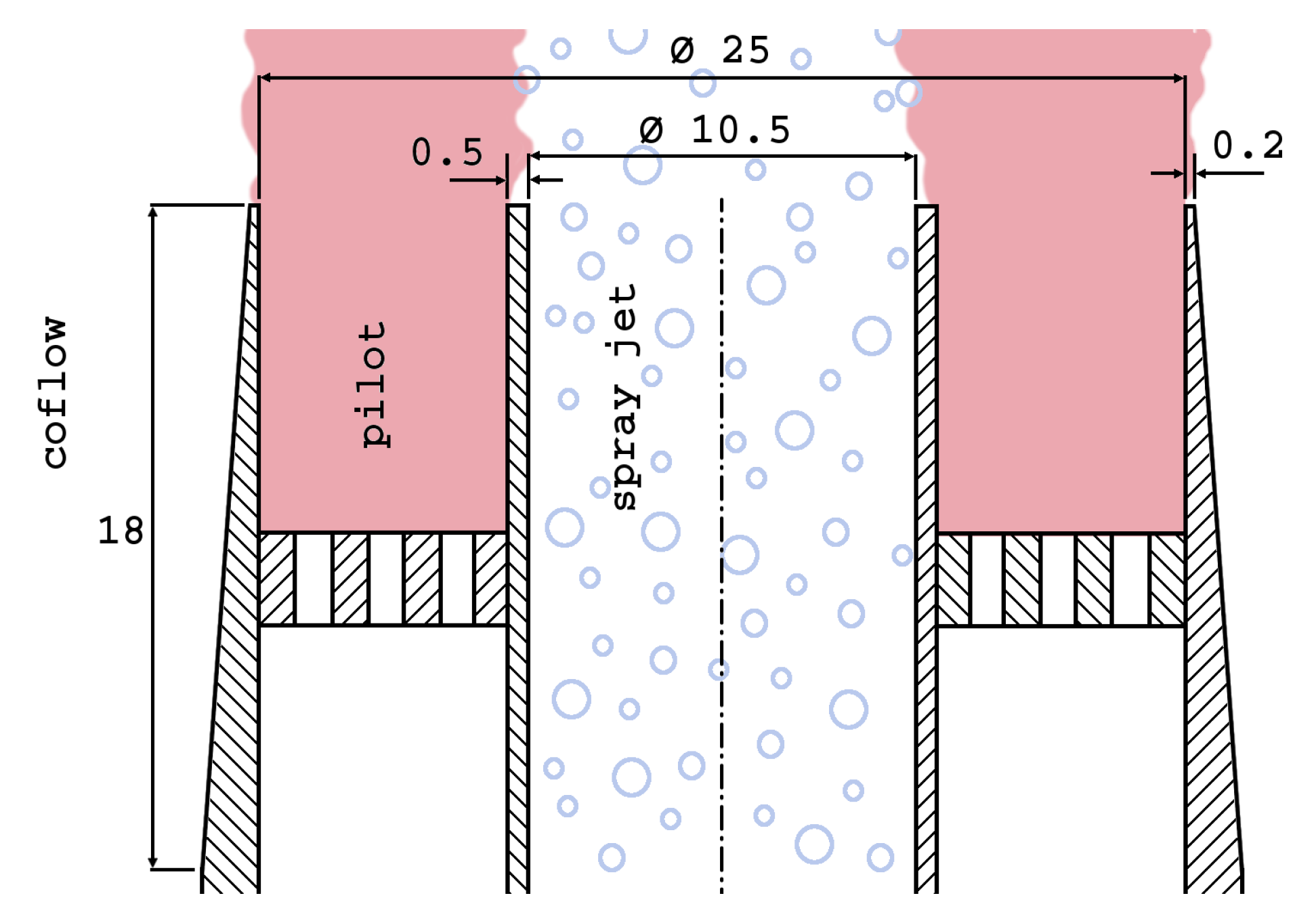
2.4. Experimental Configuration

The present investigations are performed for the flame EtF6 of the Sydney Dilute Spray Burner [39]. The burner consists of three concentrically arranged streams, namely a central jet, a pilot, and a primary coflow stream (see Figure 1). The spray is generated using an ultrasonic nebulizer placed approximately 21 central jet pipe diameters upstream of the burner exit. The droplets are then transported downstream in the central pipe with diameter D = 10.5   mm . The central jet is surrounded by an annular pilot consisting of burnt products resulting from a stoichiometric mixture of acetylene, hydrogen and air reaction. Jet and pilot are centered in a primary coflow consisting of pure air. The primary coflow has a diameter of 103   m m . The coflow is composed of pure air with an exit bulk velocity of 4.5 m · s 1 . The burner and coflow are placed in a wind tunnel with a cross-section of 290 mm × 290 mm with the same composition and velocity as the primary coflow.
To note is that two experimental data sets for the operating condition investigated are available, namely exp. A and B (see Table 1). Even though both sets delivered similar results, some deviations can be observed, thus providing an initial estimate of the experimental uncertainties. In particular, radial velocity measurements are only available for experimental set B [39,74].
The computational domain employed in this work is the same as the one described in [7] to allow for a consistent comparison of the simulations. Please note that the spatial resolution has been shown to be sufficient in [7]. The cylindrical mesh ranges 75 D downstream in axial and 10.5 D in radial direction and consists of 4.3 million hexahedral control volumes. This implies that the secondary coflow, i.e., the wind tunnel coflow, is only partially included in the computational domain. A section of 6 D upstream of the burner exit is included for the central jet to generate valuable flow conditions at the burner exit plane. Therefore, a fully developed turbulent flow has been assumed. The flow conditions have been achieved by using a recycling method, namely by mapping the velocity profile at the burner exit onto the inflow plane. As described in [7], the central jet bulk velocity has been modified to fit the mean profiles measured in the experiments. The pilot and wind tunnel streams have been assumed laminar while synthetic turbulence has been applied to the primary air coflow. Unlike in the experiment, the pilot flame composition is simplified to a burnt stoichiometric ethanol-air mixture, which is similar to the approach used in [7,8,9,42,75]. For the near wall region, the wall function formulation by Spalding [76] has been applied. All further boundaries are employing a constant total pressure formulation, which mimics the entrainment effect of the spray jet flame onto the surrounding wind tunnel coflow.
The liquid phase is injected 0.3 D downstream of the burner exit, which corresponds to the first plane where the droplet sizes have been experimentally determined. In this work, a radially conditioned size distribution is adopted, which has been obtained from experimental set A [74]. The dispersed phase velocity at injection is assumed as the carrier velocity interpolated at the droplet position. The employed injection strategy assumes an equal mass for all injected parcels. This results in a number of real droplets represented by computational parcels varying from parcel to parcel. The parcel mass at injection was estimated a priori to obtain a computationally affordable number of simultaneously tracked parcels (≈2.3 million). By using this strategy, it is also possible to inject parcels representing less than one real droplet. This is the case for droplets with larger diameters.

3. Results

In this section, the LES results obtained for the flame EtF6 using the ESF method with 8, 16 and 32 stochastic fields are investigated. The ESF simulations are subsequently abbreviated as ESF(8), ESF(16) and ESF(32), respectively. Herein, the results are first provided in terms of instantaneous contour plots before comparing the simulation results with experimental data for the gaseous and liquid phase. In this context, the ESF simulations are also compared with previous LES results presented in [7], which were performed using the Artificially Thickened Flame model. Next, time series of the table controlling variables are presented for the LES performed with 32 stochastic fields and the shape of the reconstructed marginal subgrid scalar distributions are compared with common presumed PDF shapes. Thereafter, the differences between the presumed PDF and the actual reconstructed PDF are evaluated quantitatively by comparing the PDF-integrated progress variable source term and the Hellinger distance.

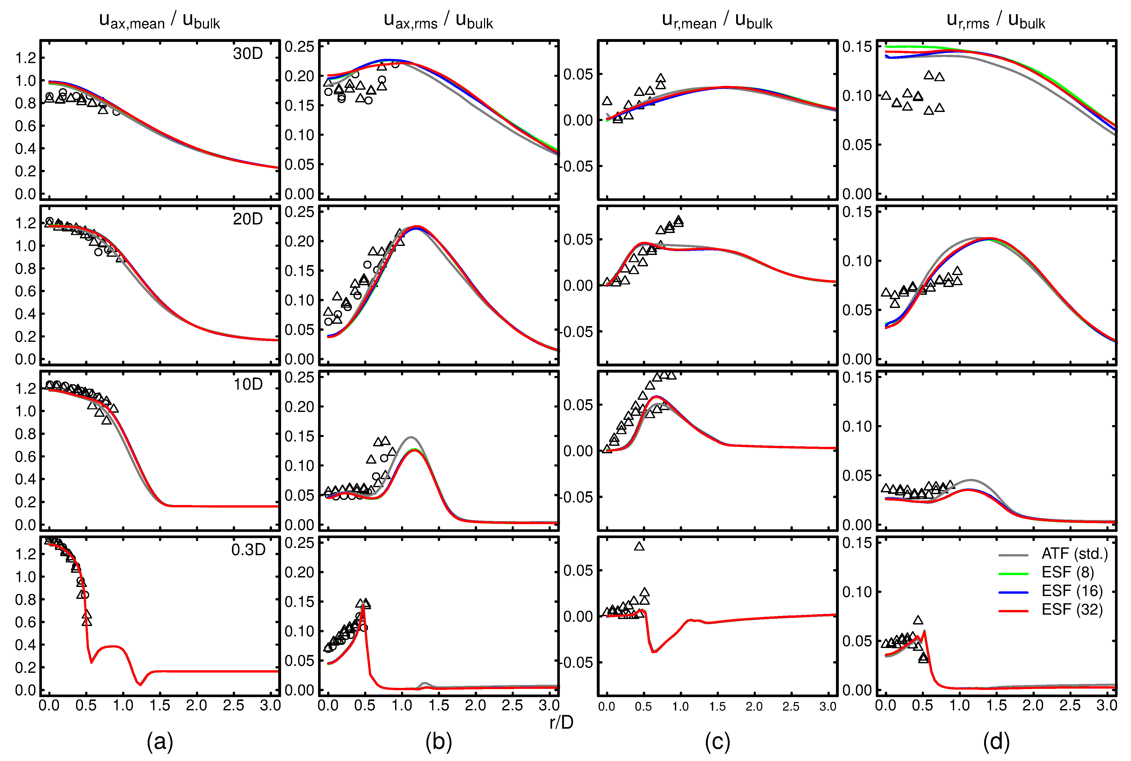
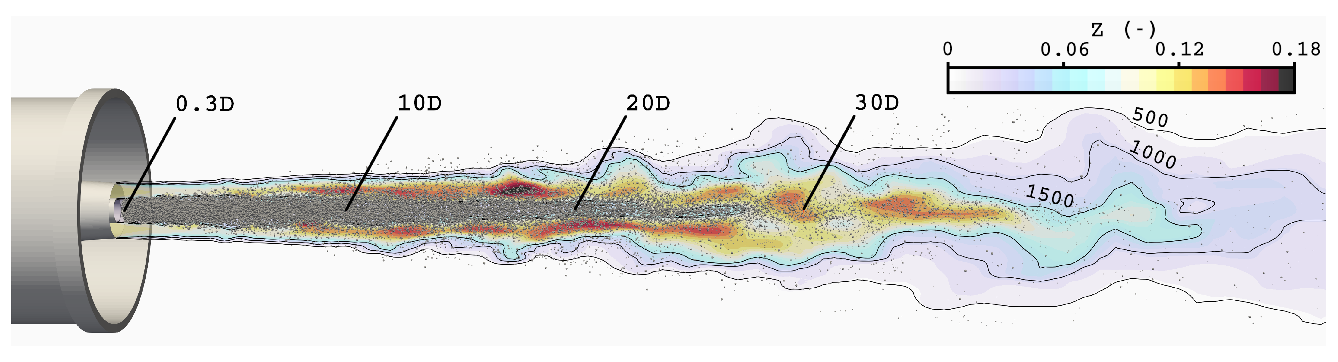
3.1. Flame Characteristics and Carrier Phase Analysis

In this part, the main features of the flame are first discussed based on instantaneous and averaged contour plots obtained from the ESF solution before going over to a comparison of the simulation results with experimentally available data. Additionally, the LES-ESF results are set aside previous results shown in [7], which were obtained using the ATF model. Since the ATF model accounts for the turbulence–chemistry interaction in the context of LES, it is also used together with experiments to appraise the ESF-based approach.
Figure 2 depicts contour plots of the FDF-integrated temperature (top) as well as the mixture fraction field (bottom) for the LES with 16 stochastic fields. Each subfigure is subdivided in its temporal average and instantaneous field, respectively, shown in the upper and lower parts. At lower axial positions, the central spray jet core and the pilot flame are concentrically arranged and the boundaries between both streams are very distinct. In this region, the cold jet core has not reached flammability and therefore hinders the pilot flame from propagating towards the center. Also to mention is the minor wrinkling effect of the shear layer on the flame. As axial distance from the burner exit increases, the flame wrinkling becomes more intense and large structures can propagate towards the centerline. This process seems to be dominated by advection as the mixture around the centerline is still below flammability. The significant increase in mixture fraction between x / D = 10 and x / D = 20 , which can be observed for mean and instantaneous contours, indicates strong evaporation of droplets. Both the higher interaction of turbulence with the flame front and a mixture evolving towards flammability promote the propagation of the reaction zone towards the centerline. This results in a cold spray core which disappears for axial distances x > 25 D . A comparison of the instantaneous contours of temperature with Figures 9–11 of [7] already suggests a stronger turbulence flame interaction for the transported PDF approach than for the ATF-based simulations. This is not unexpected as the ATF-induced flame thickening generally reduces the flame distortion caused by the turbulent eddies, yielding less spatial displacement of the flame for this approach. This impression will be confirmed later in this section by quantitatively comparing temporal rms values of temperature at various positions for the ATF and ESF-based approaches.
Next, radial profiles of carrier velocity and scalar temporal statistics are evaluated at the axial positions x / D = 0.3 , 10 , 20 , 30 , marked with green vertical lines in Figure 2. To quantify the averaging error of the temporal statistics shown, an error estimation has been performed and is presented in Appendix A. The results of the ESF simulations using 8, 16 and 32 stochastic fields are set aside experimental measurements. The simulation results are also plotted alongside results obtained using the ATF method with standard correction of heat and mass transfer of the droplet (referred to as std. correction in [7]). Since the ATF-based simulations were performed using the same framework as their ESF pendant, a comparison of the approaches makes an estimation of the impact of the flame-turbulence-interaction treatment for this flame possible. The simulation results are compared with available measurements for experimental sets A and B. It is worth noticing that the experimentally determined velocity statistics are based on droplet velocities with diameters <10 μm assuming a Stokes number well below unity. First, taking a look at the time-averaged velocity statistics of the carrier phase shown in Figure 3, at the lowest axial plane, the three distinct streams corresponding to spray jet, pilot flame, and coflow are visible in the axial velocity profile (Figure 3a). As distance from the burner exit increases, these peaks rapidly merge into each other to form one uniform profile which can then be observed at all further axial positions. The simulation results agree well with the experimental data except for the most downstream plane, where the axial velocity is overpredicted. A possible reason for this effect is the adiabatic tabulation strategy employed. Since a two-dimensional lookup table is used, any cooling effects or heat losses due to the evaporation of the spray are inherently neglected, which is likely to induce higher temperatures than in the experiment. This causes a higher thermal expansion of the carrier phase, which in turn yields higher velocities. Additionally, as will be shown next by means of the scalar statistics shown in Figure 4, the simulations tend to overestimate the length of the cold spray core. This is likely to shift the combustion reaction and the associated thermal expansion to higher axial positions. The overestimation of the length of the cold spray core will be the subject of discussion later in this section. Even though underestimating the centerline fluctuations at the lowest axial position, the standard deviation of the axial velocity seems to reproduce the experimental trends well. This behaves similarly for the radial velocity statistics with exception of radial velocity rms at the most downstream position.
Comparing the different approaches, it is possible to conclude that the flow-field is not strongly affected by the combustion model employed. Both approaches, the ATF model and the ESF-based framework are reproducing the measured velocity statistics. It is also interesting to note that the presented simulation results are not sensitive to the number of stochastic fields used. This indicates that the results reached convergence with respect to at least 8 stochastic fields used.
Figure 4 presents radial profiles of different scalar quantities at the axial positions highlighted in Figure 2. Please note that for the rms quantities, the time-averaged subgrid contributions obtained from the ESF simulations are also displayed (dashed lines in Figure 4b,d). At the lowest axial position, the distinct temperature peak corresponding to the hot flue gas of the pilot flame and the differences in mixture fraction between jet, pilot and coflow are clearly visible. Additionally, small peaks are perceivable for temperature and mixture fraction rms, resulting from the interaction with the shear layers. At this position, all approaches perform similarly. Going over to higher axial positions, the flame progresses towards the centerline, as shown by the time-averaged temperature in Figure 4a. At the same time, this temperature increase induces strong evaporation of liquid droplets, yielding an increase of the mixture fraction, which can be observed in Figure 4c. The uniform profiles of mixture fraction and temperature at the most downstream position confirm that the cold core has disappeared. Going back to the temporal averages of the excess temperature in the very left column of Figure 4, large discrepancies between the simulations and the experiments are visible at all measurement planes. First, it can be observed that the peak temperatures are overestimated at all axial positions. Nevertheless, this is consistent with the employed two-dimensional lookup table, as has been previously outlined in the discussion of the velocity profiles. The impact of the evaporative cooling on the carrier temperature has been investigated by Sacomano Filho et al. [43] for the flame EtF5 of the Sydney Spray Burner. Thereby, it has been shown that the peak carrier temperature is better matched when evaporative cooling is considered. A consideration of the evaporative cooling could be included by either using a third table dimension as the enthalpy [43,77] or through linearization of a transported energy variable [78]. The second point is related to the lower centerline temperatures perceived for all simulations when compared with experimental data. This can be observed in Figure 4a at the axial positions x = 10 D and x = 20 D . The results suggest that all simulations are underpredicting the flame propagation towards the jet center, a matter that was observed in our previous work for the ATF model [7] and in the LES shown by Heye et al. [46] for the two spray flames EtF2 and EtF6. The possible reasons for this behavior can be divided into two categories: (1) Deviations related to the modeling strategy and (2) uncertainty in boundary conditions (or a combination of both). Regarding the modeling framework, the main shortcomings related to this issue are the neglect of radiative heat transfer and the absence of differential diffusion effects. The former reduces heat diffusion in the central jet, which in turn yields lower evaporation rates of the spray. This retards the evolution of a burnable mixture and the flame propagation towards the center. The Lewis number of unity assumption is also contributing to a slower flame propagation in the central jet by omitting the forward diffusion of small species as hydrogen. The uncertainties in the boundary conditions are mainly related to the mixture composition at the burner exit. In this work as well as in previous simulations of various configurations of the Sydney Spray Burner [7,9,42,44,45,46,77], a homogeneous distribution of fuel within the spray pipe is assumed. However, depending on the flow characteristics inside the central jet, the spray dynamics may change, yielding different spatial distributions of the fuel at the burner exit (for instance, due to the development of a liquid film at the pipe walls [41]). As pointed out in the conclusions presented in [46], non-homogeneous mixtures at the burner exit may significantly impact the development and propagation of the flame front.
First disparities between the ATF and the ESF approaches arise around x = 10 D and reach their maximum at x = 20 D . At the latter position, differences are noticed for all scalar quantities shown. The results suggest that the LES-ESF predicts an earlier flame propagation of the flame towards the centerline, which is expected since these simulations move across the lower flammability limit at lower axial positions, as the averaged mixture fraction profiles suggest. The differences between the approaches are even more pronounced when considering the scalar rms profiles shown in Figure 4b,d and Figure 5. Compared to the ATF-based framework, the transported PDF-based method does predict higher rms values at all axial positions for both temperature and mixture fraction field. However, it is challenging to evaluate the differences due to the unavailability of measurements with respect to the scalar rms values. The results suggest significantly stronger variations across the possible range of values for the ESF simulations, which confirms the initial impression based on the instantaneous scalar contours shown in Figure 2 of a stronger sensitivity of the flame to turbulent motion. For instance, the centerline rms of temperature and mixture fraction for the LES-ESF approach are approximately twice as high as the LES-ATF-based modeling strategy. This indicates a higher probability of extreme events, i.e., events far away from the temporal means of the respective fields, for the ESF approach. The lower rms values perceived for the ATF approach are also consistent with the observations made in a stratified flame [31]. Regarding the rms values for the mixture fraction, both approaches do not only differ with respect to the intensity of the scalar fluctuations, but also in the shape of the profiles. This can be observed at the two axial positions x = 10 D and x = 20 D , where the ESF approach predicts a double peak structure similar to the temperature rms profile. In difference, the ATF approach produces a triple-peak-like profile, which is on one hand resulting from a reduced sensitivity of the flame to turbulent motion (or flow perturbations in general) and to the correction of heat and mass transfer of liquid droplets due to the flame thickening on the other. Additionally, one important feature of transported PDF methods is their ability to include subgrid contributions in the scalar fluctuations, shown as dashed lines in Figure 4b,d. As expected for LES, the subgrid contributions to the scalar fluctuations are much smaller than their resolved counterpart. In difference to the carrier velocity statistics, the results suggest a minor dependency of the ESF simulations regarding the number of stochastic fields used. This is most pronounced around x = 20 D at the centerline, where the ESF(8) simulation predicts the highest centerline temperatures and slightly higher temperature and mixture fraction rms. Considering the corresponding subgrid statistics, the number of stochastic fields appears not to have a strong influence. These findings are confirmed by the axial centerline profiles shown in Figure 5.

3.2. Dispersed Phase Analysis

A first qualitative impression of the liquid phase is provided in Figure 6, which presents instantaneous contours of the mixture fraction superimposed with the Lagrangian parcels representing the liquid phase. Isolines of temperature have been added to get a better notion of the hot gases. As shown in the figure and previously outlined in Section 2.4, the parcels are injected 0.3 D downstream of the burner exit plane. The parcels are then mainly traveling within the cold central core, which indicates a stronger liquid flux in this region. However, as the axial distance increases, more parcels can exit the cold core and interact with the hot pilot gases. This causes the droplets to quickly evaporate, yielding the observed gradual increase in mixture fraction. Downstream of x = 30 D , significantly less parcels can be perceived as even more droplets have evaporated.
Going over to time-averaged droplet statistics, Figure 7 presents the mean diameter D 10 , Sauter mean diameter D 32 , and liquid volumetric flux. At the most upstream plane, all fields agree well with the experimental measurements. Considering Figure 7a,b, a first observation is that as the axial distance from the burner exit increases, the representative diameters tend to be underestimated. The reason for these deviations in the characteristic diameters are two-fold: First, since the flame entrance into the spray jet occurs at higher axial distances (see Section 3.1), small droplets are more likely to be present at higher axial positions. Secondly, by simplifying the injection velocity of the parcels to the gas phase velocity [45], a low Stokes numbers for all droplets injected is being presumed. This yields higher velocities for the large particles than experimentally determined. These higher velocities eventually favor the exit of large droplets from the central jet due to their high inertia. Both effects are contributing to the lower characteristic diameters observed in the LES. Moreover, the longer cold spray core is also responsible for the overprediction of the volumetric flux at x = 20 D (Figure 7c). The differences between ATF and ESF are only visible in the liquid volumetric flux profiles at higher axial positions. These are consistent with previous findings. As can be observed in Figure 4a and Figure 5, the flame enters the central region of the spray jet at lower axial positions for the ESF method. This earlier flame propagation yields stronger evaporation rates of the spray, which become apparent in the lower liquid volumetric fluxes for this approach. As for the carrier phase analysis, only marginal differences between the stochastic field simulations can be perceived.
To sum up, considering the simplifications made in this work and the uncertainties in the boundary conditions, the observed deviations with the experimental measurements appear reasonable.

3.3. Temporal Evolution of the Subgrid Scalar PDF and Comparison with Presumed Shapes

Following the discussion and interpretation of the previous results, an in-depth analysis of the subgrid statistics is performed in the present section. The evaluations are performed for the most detailed simulation, i.e., the LES-ESF with 32 stochastic fields. The most common simplification to bypass the extensive computational costs linked to the transported PDF method is to presume the PDF shape prior to the simulation. The shape function has then to be parametrized by the moments of the distribution and it is commonly assumed that the PDF can be represented by its first two moments. It is then possible to pre-integrate the thermochemical lookup-table with the moments (usually the first one or two) of the distribution, which in turn become additional table controlling variables (thus increasing the dimensionality of the lookup-table). Herein, depending on the presumed subgrid PDF shape, additional transport equations or closures are required. However, solving one or two scalar transport equations in contrast to 8, 16 or 32 seems appealing, especially in the context of expensive spray combustion simulations. This motivates the subsequent analysis of the ESF simulations and its comparison with various presumed PDF shapes. This investigation is done based on time series of the table controlling variables at position A (see Figure 2), which is located at the centerline 20 jet diameters downstream of the burner exit plane. This position has been chosen based on the high scalar fluctuations observed for temperature and mixture fraction shown in Figure 4 and Figure 5. Please note that the following investigation is performed at a representative position (similar behavior has been observed at other positions), where a significant contribution of the subgrid terms is expected.
Before going over to a detailed analysis of the PDF shapes, a first impression of the dynamics of the subgrid fluctuations is presented in Figure 8, which depicts the time series of the mixture fraction and progress variable stochastic fields alongside their respective first moment (red line). Both fields are shown in their normalized form, which implies a normalization of each progress variable stochastic field P V i with its respective mixture fraction field Z i , yielding
c i = P V i P V m i n ( Z i ) P V m a x ( Z i ) P V m i n ( Z i ) .
A first observation is that both mixture fraction and reaction progress are subject to strong variations, which is consistent with the high temporal fluctuations of temperature and mixture fraction at the centerline shown in previous figures. In particular, the high fluctuations of the normalized progress variable exhibited in the bottom part of Figure 8 indicate rapid changes between unburned (time instant ➊) and burnt states (time instant ➋). Additionally, the paths of the stochastic fields attest strong variations of the width and shape of the subgrid PDF for both mixture fraction and normalized progress variable. Herein, it is also important to note that the mixture fraction stochastic fields extend over a significantly narrower range than the normalized reaction-progress variable. Another remarkable aspect is the apparent strong correlation of mixture fraction and reaction-progress variable, as can be deduced from the similar shape of the profiles and which is further attested by a Pearson correlation coefficient [79] for the stochastic fields of 0.87. It seems that the relative contributions of convection and diffusion, which are acting on both progress variable and mixture fraction, play a major role at this position.
The transported stochastic fields can be used to evaluate the shape of the one-time (and one-point) marginal subgrid PDFs, which is done for the time instants ➊, ➋, and ➌ displayed in Figure 8. Please note that the PDF shape is approximated by a kernel density estimation (KDE) based on the distribution of the stochastic fields. The KDE of the PDF P ^ ( x ) is created by superimposing Gaussian density kernels and satisfies the same condition as the real PDF, i.e., P ^ ( x ) 0 and 0 1 P ^ ( x ) d x = 1 . The KDEs are plotted alongside three widely used presumed PDF shapes in Figure 9. The presumed PDF shapes investigated are (1) the δ -shape, (2) a top-hat profile and (3) a β -shape (see Appendix B). Please note that the presumed shapes are all reconstructed using the first and second moments of the runtime-computed PDF obtained directly from the ESF simulations via Equations (6) and (7). The upper row of Figure 9 depicts the mixture fraction subgrid PDFs, while the lower is showing the normalized progress variable. Starting with instant ➊ shown in the left column of Figure 9, one can clearly see differences between the KDE and the presumed shapes. At this time, the mixture is below the lower flammability limit and both PDFs are narrow. Although the β -shape resembles the KDE most suitably, all presumed shapes present deviations from the KDE. This cannot be postulated for time instant ➋, where the rich mixture is almost fully burnt, as can be deduced from a mean normalized progress variable close to unity. Here, the β -shape is not too far off the real PDF KDE for both scalars and seems to perform better than the top-hat approximation. Going over to the time instant ➌ shown in the right column of Figure 9, one can observe that the KDE extends over a broader range of values for mixture fraction and normalized progress variable. For the mixture fraction, the ESF simulation predicts a subgrid distribution approximately ranging from the lower flammability limit to stoichiometry, which can be represented by a β -shape. Regarding the normalized progress variable, the distribution of the stochastic fields in Figure 8 at that time instant suggest a multi-modal shape, which is confirmed by the KDE shown in Figure 9. In this case, all presumed approaches have difficulties to approximate the ESF-based solution.
So far, only a qualitative comparison of the presumed PDFs shapes with the stochastic field simulation results has been provided. This analysis is subsequently complemented by a quantitative investigation shown in Figure 10. The figure is divided into three parts, where the first one compares the PDF-integrated source term 0 1 0 1 ω ˙ P V P ( Z , c ) d c d Z obtained from the ESF simulation with 32 stochastic fields with its pre-integrated equivalent resulting from various presumed shapes (see Appendix B). The comparison is performed over the same time period shown in Figure 8. The second part exhibits the absolute difference | Δ ω ˙ ¯ P V | between the simulation results and the a posteriori evaluated integrated source terms. Finally, the Hellinger distance H 2 (see Appendix C), which is a measure for the distance between two probability density functions, is evaluated for the marginal scalar PDFs using β and top-hat presumed shapes.
First, considering the first row of Figure 10, the non-zero values in the profile of the reaction-progress variable source term indicate regions of chemical reactions which are caused by the flame front approaching and/or crossing the probe location. In between those regions are zones where the source term is zero, which is consistent with the previously discussed temporal profiles of the stochastic fields. More precisely, the zones are mostly characterized by mixture fraction values below the lower flammability limit. The various PDF-integrated source terms resulting from the presumed shapes are plotted alongside the closed source term obtained from the stochastic fields simulation. Thereby, statistical independence of Z and c has been implicitly assumed for the presumed PDF method and the same shape function has been set for progress variable and mixture fraction. This yields three presumed joint PDF representations: (1) a double δ -, (2) a double top-hat- and (3) a double β -distribution.
As shown in the upper two rows of Figure 10, the value of the progress variable source term may vary considerably depending on which shape of the scalar subgrid PDF is assumed. Moreover, the results suggest that neglecting subgrid-scale interactions, as performed by assuming a double δ -shape, yields at most times considerably higher values of the source term compared with the ESF. The two other presumed approaches, i.e., the top-hat- and β -shape, deliver considerably lower deviations and are at some points able to reproduce the results from the stochastic fields reasonably well (see for instance the source term peak around 5 m s ). From these profiles, it is also possible to infer that the double top-hat- and double β -function presumed shapes perform almost evenly. This is especially noteworthy since the top-hat-function considerably facilitates the storage and the retrieval of the thermochemical state in the lookup table compared to its β -counterpart (see for instance [44]). Nonetheless, the integrated source term profiles corresponding to these presumed shapes also reveal substantial deviations from the ESF solution, as can be noticed exemplarily around time instant ➌, where both approaches are approximately 50% off the ESF results.
Finally, the temporal evolution of the Hellinger distance (see Appendix C) is shown in the bottom row of Figure 10 to quantify the differences between the presumed PDF shapes and the ESF results. In this context, a value of zero denotes identical functions and one indicates the maximum distance between both probability density functions compared. The Hellinger distance is computed by comparing the marginal PDFs obtained from the ESF simulation with their respective presumed shape. A first observation is that the top-hat shape produces higher distances over the whole time range considered for both Z and c, which is expected considering the qualitative comparison shown in Figure 9. A second finding is that the subgrid probability density function of mixture fraction appears to be approximated more accurately than its normalized progress variable equivalent. This can be deduced from the higher distances obtained for the normalized progress variable. Going back to the actual source term differences shown in the plot above (Figure 10, center row), one can see a correlation with the Hellinger norm. For instance, the rise in | Δ ω ˙ P V | around 3 m s and at time instant ➌ clearly have their corresponding peaks in the H 2 -profiles for the presumed PDFs of c. This finding, combined with a lower Hellinger distance for the mixture fraction presumed PDFs, confirms that the mismatch of the source terms is mainly caused by a deviation in the normalized progress variable presumed PDF shapes. Moreover, a comparison of the two lower plots of Figure 10 also reveals regions where the Hellinger distance attests high deviations in the PDF shape for both scalars, but no deviations between the presumed and transported PDF-integrated source term are found. The most striking examples for such a scenario can be found in the time range from 6 m s to 8 m s and at time instant ➊. As previously outlined, in these ranges, the mixture fraction is below the lower flammability limit and the thermochemical state does not vary strongly across the table controlling variables. In these regions, predicting the correct shape of the subgrid PDF has no impact on the closure of the reaction source term. This leads to the conclusion that deviations in PDF shapes cannot be exclusively used to evaluate the prediction ability of a presumed PDF approach. On the other side, the sole comparison of certain PDF-integrated quantities also appears reductionistic due to the neglect of error compensation effects and due to the fact that each quantity varies differently across the thermochemical lookup table. In this context, it is important to mention that in difference to the analysis presented in this work, presumed PDF approaches usually rely on closures to obtain the required moments of the marginal PDFs, which may introduce additional uncertainties. It seems that only a combination of both previously mentioned approaches, i.e., comparing the subgrid PDF integrated values and a direct comparison of the PDFs themselves with a suitable norm, can reveal the whole picture, thus helping to evaluate the prediction ability of presumed PDF shapes.

4. Conclusions

A novel strategy to perform simulations of turbulent spray combustion has been proposed in this work. The modeling framework is based on the Eulerian Stochastic Fields method coupled to the FGM tabulation strategy, while the multiphase flow is treated using a two-way coupled Euler-Lagrangian approach. The predictive capability has been demonstrated in a complex configuration, i.e., the ethanol spray flame EtF6 of the Sydney spray burner. The results have been compared with experimental measurements and previous simulations obtained using the Artificially Thickened Flame model with standard correction of droplet heat and mass transfer, as shown in [7]. It has been demonstrated that the approach is able to reproduce the temporal statistics of the flow-field reasonably well. Regarding the scalar statistics of the carrier phase, an underestimation of the flame propagation towards the jet centerline has been revealed, which is similar to the previous observations of [7,46]. Nonetheless, as can be seen from the centerline evolution of the carrier scalars shown in Figure 5, the LES-ESF simulations predict an earlier propagation of the flame towards the center of the spray jet, which comes closer to the experiments than the ATF results shown. The temporal scalar fluctuations indicate a much stronger flame-turbulence interaction for the ESF-based approach. The liquid-phase statistics are in excellent agreement with the experimental measurements at lower axial positions but differ at higher distances from the burner exit, which is consistent with the evolution of the carrier temperature. Moreover, it has been shown that the ESF results are not strongly influenced by the number of stochastic fields employed in the range investigated, which confirms previous investigations performed in purely gaseous combustion [33,80].
In a next step, the ESF simulation with 32 stochastic fields has been used to characterize the evolution of the subgrid contributions at a representative position. Thereby, the time series shown for the two table controlling variables of mixture fraction and progress variable (in its normalized form) revealed strong variations of the subgrid PDF width and shape, which has been confirmed by reconstructing the marginal subgrid PDFs at various time instants. Additionally, these one-time, one-point PDFs obtained from the ESF simulations have been compared qualitatively with common presumed density function shapes. Thereafter, this analysis has been complemented by a comparison of the PDF-integrated source term of the progress variable. It has been shown that the closed reaction-progress variable source term value is strongly connected to the presumed PDF shape. The highest deviations between source term obtained from the transported and presumed PDF have been observed for a double δ distribution and the smallest deviations for a double β -shaped PDF. Next, the temporal evolution of the Hellinger distance revealed a clear correlation with | Δ ω ˙ ¯ P V | , which is the absolute difference between computed and presumed PDF-integrated source term. The profiles also suggest that the difference in source term value is mainly caused by a deviation in the normalized progress variable presumed PDF shapes. The analysis also unveiled regions where the Hellinger distance attests high deviations in the PDF shape for both scalars, but no deviations between the presumed and transported PDF-integrated source term are found. This leads to the conclusion that quantifying the similarity of presumed and transported PDF shape is not sufficient to evaluate the prediction ability of a presumed PDF shape. On the other side, a quantification solely based on integral values for certain quantities also appears incomplete. For instance, comparing a different quantity than the progress variable source term may favor one or another presumed shape, depending on the operating condition and the respective subgrid fluctuations. The analysis demonstrates that a combination of both evaluation methods improves its informative quintessence. Nevertheless, a complete evaluation of the presumed PDF function performance and accuracy should include results obtained from simulations conducted with this approach. Furthermore, while the considered position unveiled various possible subgrid PDF shapes, many more scenarios exist. To make the present investigations more general, it remains to be shown whether the results can be transferred to other operating conditions or configurations. These aspects and the incorporation of subgrid effects on the disperse phase will be subject of future works.

Author Contributions

Conceptualization, L.D., F.L.S.F. and H.N.; Formal analysis, L.D., F.L.S.F., F.R. and H.N.; Funding acquisition, A.S.; Methodology, L.D., F.L.S.F. and F.R.; Resources, J.J. and A.S.; Software, L.D.; Supervision, J.J. and A.S.; Validation, F.R. and H.N.; Visualization, L.D., F.R. and H.N.; Writing—original draft, L.D. and F.R.; Writing—review & editing, L.D., F.L.S.F., F.R., H.N. and A.S. All authors have read and agreed to the published version of the manuscript.

Funding

This research was funded by the German Research Foundation DFG in the framework of the SFB-TRR 150 (DFG project number 237267381).

Acknowledgments

We kindly acknowledge the Darmstadt Graduate School of Energy Science and Engineering (DFG project number 194657927) as well as the Open Access Publishing Fund of the Technical University Darmstadt for the financial support. All computations were performed on the Lichtenberg High Performance Computer (HHLR) of the Technische Universität Darmstadt. We would also like to thank the group of Professor Assaad Masri, University of Sydney, for providing the validation data for all results presented.

Conflicts of Interest

The authors declare no conflict of interest.

Abbreviations

The following abbreviations are used in this manuscript:
LESLarge Eddy Simulation
DNSDirect Numerical Simulation
FGMFlamelet Generated Manifold
ATFArtificially Thickened Flame
ESFEulerian Stochastic Fields
PDFProbability Density Function
FDFFiltered Density Function
KDEKernel Density Estimation
THtop-hat

Appendix A. Estimation of Sampling Errors

In the present LES study, statistical moments (e.g., mean and rms velocities) are used to assess the performance of the proposed ESF approach in the turbulent spray flame EtF6 test case [39]. Herein, statistical moments are estimated by a finite number of sample averages over a finite time period. They consequently contain sampling errors that must be quantified to ensure estimates with a sufficient degree of accuracy.
Following the procedure described in [81,82], the sampling error of basic estimates in LES can be calculated a posteriori by means of the local mean magnitude velocity | U | , the local turbulent length scale L t and the record length t a v . In the case of the rms velocity, which can be seen as a representative statistic quantity in turbulent flows, the error measure reads
e r m s = L t | U | · t a v ,
in which the local turbulent length scale is defined as L t = k 3 / 2 / ϵ k [83]. To close Equation (A1), expressions for the total turbulent kinetic energy k and its dissipation rate ϵ k are required. In the context of LES, these quantities can be approximated as
k 1 2 u ˜ i u ˜ i + k s g s and ϵ k = τ ¯ i j u ˜ i x i + ϵ k s g s
where denotes spatial or temporal averaging. By using the inertial subrange theory, the total turbulent kinetic energy and its dissipation rate can be calculated as k s g s = ν s g s 2 / Δ 2 C K 2 and ϵ k s g s = ν s g s 3 / ( Δ 4 C S 4 ) , respectively, with C K = 0.094 and C S = 0.17 (see [82,84]).
Figure A1 presents (top) the turbulent length scale L t and (bottom) the resulting sampling error in the turbulent spray flame EtF6 test case for an averaging time of t a v = 0.25 s . LES results are exclusively shown for the simulation with eight stochastic fields ESF(8) and for the region of interest ( 0 x / D 30 , r / D 3 ). Similar results are obtained for the other cases and therefore not shown here.
As it might be expected, the turbulent length scale is small close to the injection region ( L t D ) and it increases gradually downstream (see Figure A1(top)). In line with this observation, the sampling error in Figure A1(bottom) appears small close to the injection and increases with increasing axial and radial distance. Thereby, the sampling error is smaller than 10 % in almost the entire region of interest. This error is further reduced by a factor of π · r L t + 1 for each radial position by means of spatial averaging in the azimuthal direction [81]. As a result, from the present averaging time of t a v = 0.25   s and by means of spatial averaging in the azimuthal direction, a sampling error less than 5 % for second-order statistics is likely expected in the present LES study of turbulent spray flame EtF6 test case.

Appendix B. Presumed PDF Approaches

In contrast to the ESF method, presumed PDF approaches rely on the prior assumption of a shape function for the scalar probability density distribution. The shape function has then to be parametrized by the moments of the distribution and it is often assumed that the PDF can be represented by its first two moments. However, in the case of a multidimensional probability distributions P ( ϕ ) , prescribing a feasible presumed shape turns out to be a difficult endeavor. This problem leads to the simplified assumption of statistical independence between the scalar dimensions of the PDF, thus substantially facilitating its description to the product of its marginal PDFs P ( ϕ ) P ( ϕ i ) . Therefore, if the moments of the marginal PDFs are known, it is possible to evaluate any quantity under consideration of the subgrid influence. In the case of a two-dimensional PDF of mixture fraction and reaction-progress variable, one obtains the closed progress variable source term
ω ˙ ¯ P V = ω ˙ P V ( Z , P V ) P ( Z , Z ¯ , σ Z 2 ) P ( P V , P V ¯ , σ P V 2 ) d Z d P V .
With respect to the application of the presumed PDF approach for reactive flow problems, the β -, top-hat-, and δ -shape are most widely spread. The β -shape [21] is a combination of Γ functions
P ( x , x ˜ , σ x 2 ) = Γ ( a + b ) Γ ( a ) Γ ( b ) x a 1 ( 1 x ) b 1
for which the parameter a and b are computed from the first two moments of the probability density function as
a = x ˜ x ˜ ( 1 x ˜ ) σ x 2 1 ; b = 1 x ˜ x ˜ x ˜ ( 1 x ˜ ) σ x 2 1 .
Similarly, the top-hat-shape relies on the first two moments of the PDF [85]:
P ( x , x ˜ , σ x 2 ) = x 0 if   ( x a x x b ) 0 else
with the parameters
x 0 = 1 x b x a ; x a = x ˜ 12 σ x 2 ; x b = x ˜ + 12 σ x 2 .
Each of these presumed shapes has a different physical interpretation. For instance, presuming a δ -shape for the subgrid PDF for both mixture fraction and reaction-progress variable is equivalent to assuming that ω ˙ ¯ P V = ω ˙ P V ( Z ˜ , P V ˜ ) .

Appendix C. Hellinger Distance

To estimate the differences between probability distributions, different approaches can be applied. For instance, Ihme and Pitsch [86] applied the Kullback–Leibler divergence or maximum entropy principle to derive a statistically most likely distribution (SMLD) based on DNS data. In this work, the Hellinger distance is used, which is a symmetric measure to evaluate the similarity of two probability density function P ( x ) and Q ( x ) [87]
H 2 ( P , Q ) = 1 P ( x ) Q ( x ) d x
and is bounded between zero and one, where zero indicates identical distributions and one maximum distance between P and Q ones.

References

  1. Jenny, P.; Roekaerts, D.; Beishuizen, N. Modeling of turbulent dilute spray combustion. Prog. Energy Combust. Sci. 2012, 38, 846–887. [Google Scholar] [CrossRef]
  2. Janicka, J.; Sadiki, A. Large eddy simulation of turbulent combustion systems. Proc. Combust. Inst. 2005, 30, 537–547. [Google Scholar] [CrossRef]
  3. Pitsch, H. Large Eddy Simulation of Turbulent Combustion. Ann. Rev. Fluid Mech. 2006, 38, 453–482. [Google Scholar] [CrossRef] [Green Version]
  4. Smooke, M.D. Reduced Kinetic Mechanisms and Asymptotic Approximations for Methane-Air Flames: A Topical Volume; Springer: New York, NY, USA, 1991. [Google Scholar]
  5. Kuenne, G.; Seffrin, F.; Fuest, F.; Stahler, T.; Ketelheun, A.; Geyer, D.; Janicka, J.; Dreizler, A. Experimental and numerical analysis of a lean premixed stratified burner using 1D Raman/Rayleigh scattering and large eddy simulation. Combust. Flame 2012, 159, 2669–2689. [Google Scholar] [CrossRef]
  6. Dressler, L.; Ries, F.; Kuenne, G.; Janicka, J.; Sadiki, A. Analysis of Shear Effects on Mixing and Reaction Layers in Premixed Turbulent Stratified Flames using LES coupled to Tabulated Chemistry. Combust. Sci. Technol. 2019, 1–16. [Google Scholar] [CrossRef]
  7. Dressler, L.; Sacomano Filho, F.L.; Sadiki, A.; Janicka, J. Influence of Thickening Factor Treatment on Predictions of Spray Flame Properties Using the ATF Model and Tabulated Chemistry. Flow Turbul. Combus. 2020. [Google Scholar] [CrossRef]
  8. Chrigui, M.; Masri, A.R.; Sadiki, A.; Janicka, J. Large eddy simulation of a polydisperse ethanol spray flame. Flow Turbul. Combust. 2013, 90, 813–832. [Google Scholar] [CrossRef]
  9. Sacomano Filho, F.L.; Hosseinzadeh, A.; Sadiki, A.; Janicka, J. On the interaction between turbulence and ethanol spray combustion using a dynamic wrinkling model coupled with tabulated chemistry. Combust. Flame 2020, 215, 203–220. [Google Scholar] [CrossRef]
  10. Maas, U.; Pope, S.B. Simplifying chemical kinetics: Intrinsic low-dimensional manifolds in composition space. Combust. Flame 1992, 88, 239–264. [Google Scholar] [CrossRef]
  11. Bykov, V.; Maas, U. The extension of the ILDM concept to reaction–diffusion manifolds. Combust. Theory Model. 2007, 11, 839–862. [Google Scholar] [CrossRef]
  12. Pierce, C.D.; Moin, P. Progress-variable approach for large-eddy simulation of non-premixed turbulent combustion. J. Fluid Mech. 2004, 504, 73–97. [Google Scholar] [CrossRef]
  13. Gicquel, O.; Darabiha, N.; Thévenin, D. Laminar premixed hydrogen/air counterflow flame simulations using flame prolongation of ILDM with differential diffusion. Proc. Combust. Inst. 2000, 28, 1901–1908. [Google Scholar] [CrossRef]
  14. Fiorina, B.; Gicquel, O.; Vervisch, L.; Carpentier, S.; Darabiha, N. Approximating the chemical structure of partially premixed and diffusion counterflow flames using FPI flamelet tabulation. Combust. Flame 2005, 140, 147–160. [Google Scholar] [CrossRef]
  15. Van Oijen, J.A.; De Goey, L.P.H. Modelling of premixed laminar flames using flamelet-generated manifolds. Combust. Sci. Technol. 2000, 161, 113–137. [Google Scholar] [CrossRef] [Green Version]
  16. Kerstein, A.R.; Ashurst, W.T.; Williams, F.A. Field equation for interface propagation in an unsteady homogeneous flow field. Phys. Rev. A 1988, 37, 2728. [Google Scholar] [CrossRef] [PubMed]
  17. Pitsch, H.; Duchamp de Lageneste, L. Large-eddy simulation of premixed turbulent combustion using a level-set approach. Proc. Combust. Inst. 2002, 29, 2001–2008. [Google Scholar] [CrossRef] [Green Version]
  18. Butler, T.; O’Rourke, P. A numerical method for two dimensional unsteady reacting flows. Symp. Int. Combust. 1977, 16, 1503–1515. [Google Scholar] [CrossRef] [Green Version]
  19. Legier, J.P.; Poinsot, T.; Veynante, D. Dynamically thickened flame LES model for premixed and non-premixed turbulent combustion. In Proceedings of the Summer Program; Center for Turbulence Research: Stanford, CA, USA, 2000; Volume 12. [Google Scholar]
  20. Pope, S.B. PDF methods for turbulent reactive flows. Prog. Energy Combus. Sci. 1985, 11, 119–192. [Google Scholar] [CrossRef]
  21. Rhodes, R.P. A probability distribution function for turbulent flows. In Turbulent Mixing in Nonreactive and Reactive Flows; Springer: New York, NY, USA, 1975; pp. 235–241. [Google Scholar] [CrossRef]
  22. Pope, S.B. A Monte Carlo method for the PDF equations of turbulent reactive flow. Combust. Sci. Technol. 1981, 25, 159–174. [Google Scholar] [CrossRef]
  23. Pollack, M.; Ferraro, F.; Janicka, J.; Hasse, H. Evaluation of Quadrature-based Moment Methods in turbulent premixed combustion. Proc. Combust. Inst. 2020. [Google Scholar] [CrossRef]
  24. Valiño, L. A field Monte Carlo formulation for calculating the probability density function of a single scalar in a turbulent flow. Flow Turbul. Combust. 1998, 60, 157–172. [Google Scholar] [CrossRef]
  25. Valiño, L.; Mustata, R.; Letaief, K.B. Consistent behavior of Eulerian Monte Carlo fields at low Reynolds numbers. Flow Turbul. Combust. 2016, 96, 503–512. [Google Scholar] [CrossRef]
  26. Sabel’nikov, V.A.; Soulard, O. Rapidly decorrelating velocity-field model as a tool for solving one-point Fokker-Planck equations for probability density functions of turbulent reactive scalars. Phys. Rev. E 2005, 72, 016301. [Google Scholar] [CrossRef] [PubMed]
  27. Sabel’nikov, V.; Soulard, O. Eulerian (Field) Monte Carlo Methods for Solving PDF Transport Equations in Turbulent Reacting Flows. In Handbook of Combustion; American Cancer Society: Atlanta, GA, USA, 2010; Chapter 4; pp. 75–119. [Google Scholar] [CrossRef]
  28. Garmory, A. Micromixing Effects in Atmospheric Reacting Flows. Ph.D. Thesis, University of Cambridge, Cambridge, UK, 2008. [Google Scholar]
  29. Jones, W.P.; Prasad, V.N. Large Eddy Simulation of the Sandia Flame Series (D–F) using the Eulerian stochastic field method. Combust. Flame 2010, 157, 1621–1636. [Google Scholar] [CrossRef]
  30. Mahmoud, R.; Jangi, M.; Ries, F.; Fiorina, B.; Janicka, J.; Sadiki, A. Combustion Characteristics of a Non-Premixed Oxy-Flame Applying a Hybrid Filtered Eulerian Stochastic Field/Flamelet Progress Variable Approach. Appl. Sci. 2019, 9, 1320. [Google Scholar] [CrossRef] [Green Version]
  31. Avdić, A.; Kuenne, G.; di Mare, F.; Janicka, J. LES combustion modeling using the Eulerian stochastic field method coupled with tabulated chemistry. Combust. Flame 2017, 175, 201–219. [Google Scholar] [CrossRef]
  32. Fredrich, D.; Jones, W.P.; Marquis, A.J. The stochastic fields method applied to a partially premixed swirl flame with wall heat transfer. Combust. Flame 2019, 205, 446–456. [Google Scholar] [CrossRef]
  33. Hansinger, M.; Zirwes, T.; Zips, J.; Pfitzner, M.; Zhang, F.; Habisreuther, P.; Bockhorn, H. The Eulerian Stochastic Fields Method Applied to Large Eddy Simulations of a Piloted Flame with Inhomogeneous Inlet. Flow Turbul. Combust. 2020, 1–31. [Google Scholar] [CrossRef]
  34. Hansinger, M.; Pfitzner, M.; Sabelnikov, V. LES of oxy-fuel jet flames using the Eulerian Stochastic Fields method with differential diffusion. Proc. Combust. Inst. 2020. [Google Scholar] [CrossRef]
  35. Jones, W.P.; Marquis, A.J.; Vogiatzaki, K. Large-eddy simulation of spray combustion in a gas turbine combustor. Combust. Flame 2014, 161, 222–239. [Google Scholar] [CrossRef]
  36. Jones, W.P.; Marquis, A.J.; Noh, D. LES of a methanol spray flame with a stochastic sub-grid model. Proc. Combust. Inst. 2015, 35, 1685–1691. [Google Scholar] [CrossRef] [Green Version]
  37. Gallot-Lavallée, S.; Jones, W.P. Large eddy simulation of spray auto-ignition under EGR conditions. Flow Turbul. Combust. 2016, 96, 513–534. [Google Scholar] [CrossRef] [Green Version]
  38. Gallot-Lavallée, S.; Jones, W.P.; Marquis, A.J. Large Eddy Simulation of an ethanol spray flame under MILD combustion with the stochastic fields method. Proc. Combust. Inst. 2017, 36, 2577–2584. [Google Scholar] [CrossRef] [Green Version]
  39. Gounder, J.D.; Kourmatzis, A.; Masri, A.R. Turbulent piloted dilute spray flames: Flow fields and droplet dynamics. Combust. Flame 2012, 159, 3372–3397. [Google Scholar] [CrossRef]
  40. Masri, A.R.; Gounder, J.D. Turbulent spray flames of acetone and ethanol approaching extinction. Combust. Sci. Technol. 2010, 182, 702–715. [Google Scholar] [CrossRef]
  41. Masri, A.R.; Gounder, J.D. Details and complexities of boundary conditions in turbulent piloted dilute spray jets and flames. In Experiments and Numerical Simulations of Diluted Spray Turbulent Combustion; Springer: New York, NY, USA, 2011; pp. 41–68. [Google Scholar] [CrossRef]
  42. Sacomano Filho, F.L.; Kadavelil, J.; Staufer, M.; Sadiki, A.; Janicka, J. Analysis of LES-based combustion models applied to an acetone turbulent spray flame. Combust. Sci. Technol. 2018, 191, 54–67. [Google Scholar] [CrossRef]
  43. Sacomano Filho, F.L.; Dressler, L.; Hosseinzadeh, A.; Sadiki, A.; Krieger Filho, G.C. Investigations of Evaporative Cooling and Turbulence Flame Interaction Modeling in Ethanol Turbulent Spray Combustion Using Tabulated Chemistry. Fluids 2019, 4, 187. [Google Scholar] [CrossRef] [Green Version]
  44. Rittler, A.; Proch, F.; Kempf, A.M. LES of the Sydney piloted spray flame series with the PFGM/ATF approach and different sub-filter models. Combust. Flame 2015, 162, 1575–1598. [Google Scholar] [CrossRef]
  45. Heye, C.; Raman, V.; Masri, A.R. LES/probability density function approach for the simulation of an ethanol spray flame. Proc. Combust. Inst. 2013, 34, 1633–1641. [Google Scholar] [CrossRef]
  46. Heye, C.R.; Kourmatzis, A.; Raman, V.; Masri, A.R. A comparative study of the simulation of turbulent ethanol spray flames. In Experiments and Numerical Simulations of Turbulent Combustion of Diluted Sprays; Springer: New York, NY, USA, 2014; pp. 31–54. [Google Scholar] [CrossRef]
  47. Nicoud, F.; Toda, H.B.; Cabrit, O.; Bose, S.; Lee, J. Using singular values to build a subgrid-scale model for large eddy simulations. Phys. Fluids 2011, 23, 085106. [Google Scholar] [CrossRef] [Green Version]
  48. Marinov, N.M. A detailed chemical kinetic model for high temperature ethanol oxidation. Int. J. Chem. Kinet. 1999, 31, 183–220. [Google Scholar] [CrossRef]
  49. Frost, V.A. Model of a turbulent, diffusion-controlled flame jet. Fluid Mech. Soviet Res. 1975, 4, 124–133. [Google Scholar]
  50. Dopazo, C.; O’Brien, E.E. Functional formulation of nonisothermal turbulent reactive flows. Phys. Fluids 1974, 17, 1968–1975. [Google Scholar] [CrossRef] [Green Version]
  51. O’brien, E.E. The probability density function (pdf) approach to reacting turbulent flows. In Turbulent Reacting Flows; Springer: New York, NY, USA, 1980; pp. 185–218. [Google Scholar] [CrossRef]
  52. Villermaux, J.; Falk, L. A generalized mixing model for initial contacting of reactive fluids. Chem. Eng. Sci. 1994, 49, 5127–5140. [Google Scholar] [CrossRef]
  53. Kloeden, P.E.; Platen, E. Numerical Solution of Stochastic Differential Equations; Springer Science & Business Media: New York, NY, USA, 1992. [Google Scholar] [CrossRef] [Green Version]
  54. Picciani, M.A. Investigation of Numerical Resolution Requirements of the Eulerian Stochastic Fields and the Thickened Stochastic Field Approach. Ph.D. Thesis, University of Southampton, Southampton, UK, 2018. [Google Scholar]
  55. Schlichting, H.; Gersten, K. Boundary-Layer Theory; Springer: New York, NY, USA, 2017. [Google Scholar]
  56. Yuen, M.C.; Chen, L.W. On drag of evaporating liquid droplets. Combust. Sci. Technol. 1976. [Google Scholar] [CrossRef]
  57. Miller, R.S.; Harstad, K.; Bellan, J. Evaluation of equilibrium and non-equilibrium evaporation models for many-droplet gas-liquid flow simulations. Int. J. Multiph. Flow 1998, 24, 1025–1055. [Google Scholar] [CrossRef]
  58. Noh, D.; Gallot-Lavallée, S.; Jones, W.P.; Navarro-Martinez, S. Comparison of droplet evaporation models for a turbulent, non-swirling jet flame with a polydisperse droplet distribution. Combust. Flame 2018, 194, 135–151. [Google Scholar] [CrossRef] [Green Version]
  59. Bellan, J.; Summerfield, M. Theoretical examination of assumptions commonly used for the gas phase surrounding a burning droplet. Combust. Flame 1978, 33, 107–122. [Google Scholar] [CrossRef]
  60. Knudsen, E.; Shashank.; Pitsch, H. Modeling partially premixed combustion behavior in multiphase LES. Combust. Flame 2015, 162, 159–180. [Google Scholar] [CrossRef]
  61. Abramzon, B.; Sirignano, W.A. Droplet vaporization model for spray combustion calculations. Int. J. Heat Mass Transf. 1989, 32, 1605–1618. [Google Scholar] [CrossRef]
  62. Wilke, C.R. A viscosity equation for gas mixtures. J. Chem. Phys. 1950, 18, 517–519. [Google Scholar] [CrossRef]
  63. McBride, B.J.; Gordon, S.; Reno, M.A. Coefficients for Calculating Thermodynamic and Transport Properties of Individual Species; NASA Technical Memorandum 4513; NASA Langley Research Center: Hampton, VA, USA, 1993. [Google Scholar]
  64. Weller, H.G.; Tabor, G.; Jasak, H.; Fureby, C. A tensorial approach to computational continuum mechanics using object-oriented techniques. Comput. Phys. 1998, 12, 620. [Google Scholar] [CrossRef]
  65. Ries, F.; Obando, P.; Shevchuck, I.; Janicka, J.; Sadiki, A. Numerical analysis of turbulent flow dynamics and heat transport in a round jet at supercritical conditions. Int. J. Heat Fluid Flow 2017, 66, 172–184. [Google Scholar] [CrossRef]
  66. Issa, R.I. Solution of the implicitly discretised fluid flow equations by operator-splitting. J. Comput. Phys. 1986, 62, 40–65. [Google Scholar] [CrossRef]
  67. Patankar, S.V.; Spalding, D.B. A calculation procedure for heat, mass and momentum transfer in three-dimensional parabolic flows. In Numerical Prediction of Flow, Heat Transfer, Turbulence and Combustion; Elsevier: Amsterdam, The Netherlands, 1983; pp. 54–73. [Google Scholar] [CrossRef]
  68. Roe, P.L. Characteristic-based schemes for the Euler equations. Ann. Rev. Fluid Mech. 1986, 18, 337–365. [Google Scholar] [CrossRef]
  69. Muradoglu, M.; Jenny, P.; Pope, S.B.; Caughey, D.A. A consistent hybrid finite-volume/particle method for the PDF equations of turbulent reactive flows. J. Comput. Phys. 1999, 154, 342–371. [Google Scholar] [CrossRef] [Green Version]
  70. Raman, V.; Pitsch, H.; Fox, R.O. Hybrid large-eddy simulation/Lagrangian filtered-density-function approach for simulating turbulent combustion. Combust. Flame 2005, 143, 56–78. [Google Scholar] [CrossRef]
  71. Raman, V.; Pitsch, H. A consistent LES/filtered-density function formulation for the simulation of turbulent flames with detailed chemistry. Proc. Combust. Inst. 2007, 31, 1711–1719. [Google Scholar] [CrossRef]
  72. James, S.; Zhu, J.; Anand, M.S. Large eddy simulations of turbulent flames using the filtered density function model. Proc. Combust. Inst. 2007, 31, 1737–1745. [Google Scholar] [CrossRef]
  73. Prasad, V.N. Large Eddy Simulation of Partially Premixed Turbulent Combustion. Ph.D. Thesis, Imperial College London, University of London, London, UK, 2011. [Google Scholar]
  74. Clean Combustion Research Group Database, University of Sydney. Available online: http://web.aeromech.usyd.edu.au/thermofluids/database.php (accessed on 23 July 2019).
  75. De, S.; Lakshmisha, K.N.; Bilger, R.W. Modeling of nonreacting and reacting turbulent spray jets using a fully stochastic separated flow approach. Combust. Flame 2011, 158, 1992–2008. [Google Scholar] [CrossRef]
  76. Spalding, D.B. A single formula for the “law of the wall”. J. Appl. Mech. 1961, 28, 455–458. [Google Scholar] [CrossRef]
  77. Sacomano Filho, F.L. Novel Approach toward the Consistent Simulation of Turbulent Spray Flames Using Tabulated Chemistry. Ph.D. Thesis, Technische Universität Darmstadt, Darmstadt, Germany, 2017. [Google Scholar]
  78. Franzelli, B.; Vié, A.; Boileau, M.; Fiorina, B.; Darabiha, N. Large Eddy Simulation of Swirled Spray Flame Using Detailed and Tabulated Chemical Descriptions. Flow Turbul. Combust. 2016, 98, 633–661. [Google Scholar] [CrossRef]
  79. Benesty, J.; Chen, J.; Huang, Y.; Cohen, I. Pearson correlation coefficient. In Noise Reduction in Speech Processing; Springer: New York, NY, USA, 2009; pp. 1–4. [Google Scholar] [CrossRef]
  80. Mustata, R.; Valino, L.; Jimenez, C.; Jones, W.P.; Bondi, S. A Probability Density Function Eulerian Monte Carlo Field Method for Large Eddy Simulations: Applications to a Turbulent Piloted Methane/Air Diffusion Flame (Sandia D). Combust. Flame 2006, 145, 88–104. [Google Scholar] [CrossRef]
  81. Ries, F.; Nishad, K.; Dressler, L.; Janicka, J.; Sadiki, A. Evaluating large eddy simulation results based on error analysis. Theor. Comput. Fluid Dyn. 2018, 32, 733–752. [Google Scholar] [CrossRef] [Green Version]
  82. Ries, F. Numerical Modeling and Prediction of Irreversibilities in Sub- and Supercritical Turbulent Near-Wall Flows. Ph.D. Thesis, Technical University of Darmstadt, Darmstadt, Germany, 2018. [Google Scholar]
  83. Pope, S.B. Ten questions concerning the large-eddy simulation of turbulent flows. N. J. Phys. 2004, 6, 35. [Google Scholar] [CrossRef] [Green Version]
  84. Ries, F.; Nishad, K.; Janicka, J.; Sadiki, A. Entropy generation analysis and thermodynamic optimization of jet impingement cooling using large eddy simulation. Entropy 2019, 19, 129. [Google Scholar] [CrossRef] [Green Version]
  85. Floyd, J.; Kempf, A.M.; Kronenburg, A.; Ram, R.H. A simple model for the filtered density function for passive scalar combustion LES. Combust. Theory Model. 2009, 13, 559–588. [Google Scholar] [CrossRef]
  86. Ihme, M.; Pitsch, H. Prediction of extinction and reignition in nonpremixed turbulent flames using a flamelet/progress variable model: 1. A priori study and presumed PDF closure. Combust. Flame 2008, 155, 70–89. [Google Scholar] [CrossRef]
  87. Cramér, H. Mathematical Methods of Statistics; Princeton University Press: Princeton, NJ, USA, 1999. [Google Scholar]
Figure 1. Schematics of the Sydney Spray Burner exit, dimensions in mm. The red colored area sketches the hot pilot consisting of burnt products.
Fluids 06 00050 g001
Figure 2. Temporal average (upper part) and instantaneous contours (lower part) of both the Favre-filtered Probability Density Function FDF-integrated temperature (top) and first moment of the mixture fraction FDF (bottom) for the Eulerian Stochastic Fields (ESF16) simulation. The vertical green bars denote axial positions at which simulation data are compared with experiments. The magenta-colored point exhibits the position of probe A, for which time-series analyses are performed in a later section.
Fluids 06 00050 g002
Figure 3. Mean and rms of resolved axial and radial velocity component at various axial distances from the burner exit compared with experimental data (○: Exp. set A; △: Exp. set B). Radial velocity statistics only available for experimental set B. (a) axial velocity mean; (b) axial velocity rms; (c) radial velocity mean; (d) radial velocity rms.
Fluids 06 00050 g003
Figure 4. Mean excess temperature (a), temperature rms (b) along with mixture fraction mean (c) and rms (d) at various axial distances from the burner exit compared with available experimental data. The dashed lines correspond to the unresolved contributions obtained from the LES-ESF simulations. The horizontal grey dotted line shown in (c) correspond to lower flammability and stoichiometry. ○: Exp. set A.
Fluids 06 00050 g004
Figure 5. Axial evolution of temporal averages and rms of temperature (a) and mixture fraction (b) along the centerline. The dashed line corresponds to total rms while the dotted line represent the unresolved contributions obtained from the LES-ESF simulations.
Fluids 06 00050 g005
Figure 6. Instantaneous contours of mixture fraction superimposed with the Lagrangian parcels alongside isolines of temperature ( T = 500 , 1000 , 1500 K ) for ESF(32).
Fluids 06 00050 g006
Figure 7. (a) Sauter mean diameter D 32 , (b) mean diameter D 10 and (c) liquid volumetric flux at various axial distances from the burner exit compared with available experimental data. ○: Exp. set A; △: Exp. set B.
Fluids 06 00050 g007
Figure 8. Temporal evolution of mixture fraction (top) and normalized progress variable (bottom) stochastic fields (grey lines) alongside their respective first moment, i.e., their arithmetic mean (red lines). The probe is located at the centerline, 20 diameters downstream of the burner exit plane. The position is displayed in Figure 2. The vertical dotted lines indicate three representative time instants, which will be discussed subsequently.
Fluids 06 00050 g008
Figure 9. Comparison of common presumed subgrid PDF shapes and kernel density estimation (KDE) approximation of the PDF obtained from the ESF simulation with 32 stochastic fields at the various time instants displayed in Figure 8 at the probe position A shown in Figure 2.
Fluids 06 00050 g009
Figure 10. Top: Temporal evolution of the PDF-integrated progress variable source term ω ˙ ¯ P V at the location of Probe A for the ESF simulations alongside results obtained from three presumed PDF shapes. Center: Absolute difference between the presumed approaches and the ESF(32) simulation results. Bottom: Hellinger distance (see Appendix C) between the stochastic fields PDF and the presumed shapes. Vertical dotted lines: time instants corresponding to the time instant discussed previously.
Fluids 06 00050 g010
Figure A1. Predicted (top) turbulent length scale L t and (bottom) sampling error e r m s for an averaging time of t a v = 0.25 s . LES results obtained with eight stochastic fields (ESF(8)).
Fluids 06 00050 g0a1
Table 1. Operating conditions for the investigated case [39,74].
Operating ConditionsEtF6
exp. Aexp. B
Bulk jet velocity (m/s)3636
Jet Reynolds number27,40027,400
Overall equivalence ratio ϕ 1.81.8
Carrier mass flow rate (g/min)225225
Liquid fuel injection rate (g/min)4545
Liquid flow rate at jet exit (g/min)41.341.1
Vapor flow rate at jet exit (g/min)3.93.7
Equivalence ratio at jet exit ϕ j e t 0.150.2
Publisher’s Note: MDPI stays neutral with regard to jurisdictional claims in published maps and institutional affiliations.

