
Performance Assessment of Fluidic Oscillators Tested on the NASA Hump Model †

NASA Langley Research Center, Hampton, VA 23681, USA
†
This paper is an extended version of “Application of Sweeping Jet Actuators on the NASA Hump Model and Comparison with CFDVAL2004 Experiments” paper published at the 47th AIAA Fluid Dynamics Conference, AIAA AVIATION Forum, Denver, CO, USA, 5–9 June 2017.
Fluids 2021, 6(2), 74; https://0-doi-org.brum.beds.ac.uk/10.3390/fluids6020074
Submission received: 6 January 2021
/
Revised: 29 January 2021
/
Accepted: 3 February 2021
/
Published: 7 February 2021
(This article belongs to the Special Issue Fluidic Oscillators-Devices and Applications)
Abstract
:Flow separation control over a wall-mounted hump model was studied experimentally to assess the performance of fluidic oscillators (sweeping jet actuators). An array of fluidic oscillators was used to control flow separation. The results showed that the fluidic oscillators were able to achieve substantial control over the separated flow by increasing the upstream suction pressure and downstream pressure recovery. Using the data available in the literature, the performance of the fluidic oscillators was compared to other active flow control (AFC) methods such as steady blowing, steady suction, and zero-net-mass-flux (ZNMF) actuators. Several integral parameters, such as the inviscid flow comparison coefficient, pressure drag coefficient, and modified normal force coefficient, were used as quality metrics in the performance comparison of the AFC methods. These quality metrics indicated the superiority of the steady suction method, especially at lower excitation amplitudes that is followed by the fluidic oscillators, steady blowing, and the ZNMF actuators, respectively. An aerodynamic figure of merit (AFM) was also constructed using the integral parameters and AFC power usage. The AFM results revealed that, for this study, steady suction was the most efficient AFC method at lower excitation amplitudes. The steady suction loses its efficiency as the excitation amplitude increases, and the fluidic oscillators become the most efficient AFC method. Both the steady suction and the fluidic oscillators have an AFM > 1 for the range tested in this study, indicating that they provide a net benefit when the AFC power consumption is also considered. On the other hand, both the steady blowing and ZNMF actuators were found to be inefficient AFC methods (AFM < 1) for the current configuration. Although they improved the flow field by controlling flow separation, the power requirement was more than their benefit.
1. Introduction
Flow separation is the detachment of fluid from a surface, for example, due to an adverse pressure gradient. It can be encountered in many engineering applications such as aircraft wings, high-lift systems, helicopter rotors, turbo machinery blades, diffusers, etc. Flow separation causes significant loss in the performance of the aforementioned systems in the form of reduced lift, increased drag, reduced pressure recovery, etc. Flow separation control, historically referred to as boundary layer control, involves manipulating the near wall fluid to delay, reduce, or sometimes completely prevent flow separation. Developing methods to control flow separation could help regain or improve the performance of fluid systems. Various active and passive flow control concepts have been proposed in the literature to control flow separation including, but not limited to, steady suction [1], tangential blowing, passive vortex generators [2], oscillatory-blowing valves [3], plasma actuators [4,5], zero-net-mass-flux actuators (ZNMF) [6], and fluidic oscillators [7]. Efficiency, complexity, and maintainability are key factors that prevent widespread utilization of these proven separation control techniques [1]. In the context of efficiency, it is generally accepted that an unsteady excitation is much more effective than steady flow control techniques to achieve a prescribed performance improvement [3]. Out of these various techniques, the fluidic oscillators, sometimes referred to as sweeping jet (SWJ) actuators, have proven to be simple, reliable, and efficient flow-control devices that can generate spatially and temporally oscillating (i.e., unsteady) jets without having any moving components.
Although there is a growing interest in fluidic oscillators as a flow control device, there are only a few studies that have investigated how well the fluidic oscillators perform compared to the other active flow control (AFC) methods. For example, the fluidic oscillators were used to control flow separation on an adverse pressure gradient ramp [8,9], and it was shown that they are more efficient than steady discrete blowing and steady vortex-generating jets. The fluidic oscillators were also compared to two-dimensional steady blowing and pulsed blowing on a highly separated transonic diffuser. It was reported that the fluidic oscillators and pulsed blowing are more efficient than the steady two-dimensional slot blowing, although both provided comparable performance [10]. A similar study [11] compared the fluidic oscillators to steady jet blowing at various spacing and input parameters. The results confirmed that the fluidic oscillators perform better than steady jet blowing. The superiority of the fluidic oscillators to the steady jet blowing was also shown for three-dimensional configurations by controlling the flow separation on a deflected flap at low [12] and high [13] Reynolds number tests.
The overall objective of the present study is to assess the performance of the fluidic oscillators in controlling flow separation. The first step in this assessment is to present the flow separation control effectiveness of the fluidic oscillators over the wall-mounted hump model. The second step involves the performance comparison of the fluidic oscillators to the existing AFC methods using the data available in the literature. The performance comparison of different AFC methods requires a quality metric to be evaluated. Therefore, another objective of this study is to present and discuss possible quality metrics that can be applied, specifically, to wall-mounted wind tunnel models. AFC system efficiency is a key factor for the implementation of AFC actuators. Therefore, an aerodynamic figure of merit, which also accounts for the actuator power consumption, is constructed using the integral parameters, and different AFC actuators are compared based on their system efficiency.
2. Materials and Methods
2.1. Experimental Setup
The wind tunnel model is the wall-mounted hump (Figure 1a), which has been used as a benchmark case for computational fluid dynamics (CFD) validation. The model was one of the case studies in the CFD Validation of Synthetic Jets and Turbulent Separation Control Workshop in 2004 and is well documented both experimentally [1,14,15] and numerically [16] over a wide range of Reynolds numbers (0.4 × 10⁶ < Re < 26 × 106). The hump model, which is the suction side of the Glauert Glass II airfoil [17], is the same model that was used by Greenblatt et al. [14,15] in the same wind tunnel. The details about the model and wind tunnel conditions can be found in Ref. [14]. Only a brief summary will be given for completeness. The characteristic length is defined as the hump chord, which is c = 420 mm. The original model had a two-dimensional slot located at x/c = 0.65 that was connected to an interior plenum spanning the entire model width (s = 584 mm) between the forebody and ramp. In order to accommodate the fluidic oscillators and the steady blowing nozzles, the stainless steel slot-lip section was refabricated. The slot-lip section was divided into two sections, where the top section housed the surface static pressure ports and the bottom section housed the fluidic oscillator array. The actuator layer extended to the model ramp section such that it sealed the existing plenum on the model surface. The data reported in Ref. [14] was acquired while there was a suction manifold under the splitter plate. In the current experimental configuration, the suction manifold was removed, and the plenum was sealed by a base plate to minimize the blockage.
The experiments were conducted in the National Aeronautics and Space Administration (NASA) Langley Shear Flow Tunnel, which is an atmospheric, open-return wind tunnel. The experimental configuration was chosen to match to that of Ref. [14]. The model was mounted on a splitter plate between two endplates and experiments were performed mostly at a freestream Mach number of 0.1, which corresponded to Rec = 0.94 × 10⁶ based on the hump chord. The boundary layer was tripped near the leading edge of the splitter plate using 20 mm thick (no. 60 grit) sand paper. Oilflow visualizations were performed prior to the wind tunnel tests to confirm that there was not a separation bubble at the leading edge of the splitter plate.
Surface static and dynamic pressures were acquired in this study. The model has 124 static pressure ports (0.5 mm orifice diameter) along the centerline and 16 spanwise pressure ports both on the forebody (x/c = 0.19) and on the ramp (x/c = 0.86) sections (Figure 2). The static pressure ports were connected to electronically scanned pressure modules. Sixteen unsteady pressure transducers were used to acquire fluctuating pressures in the separated flow region on the ramp section. Most of the dynamic pressure ports were aligned 25 mm (1 inch) off the centerline with the exception of first three ports. These were at x/c = 0.69, x/c = 0.71, and x/c = 0.73 and aligned 38 mm (1.5 inches), 51 mm (2 inches), and 64 mm (2.5 inches) off the centerline, respectively. These three pressure ports were installed to detect any three-dimensional unsteady flow structures near the actuator exits. The last three pressure ports were located along the centerline (see port locations in Figure 2). Miniature piezoresistive pressure transducers (±6.9 kPa, 1 psig) were directly attached to the dynamic pressure ports.
Oilflow visualization was performed to map the surface flow patterns. The surface flow visualization was obtained using a mixture of kerosene, aviation oil, and fumed silica particles. Details of the flow visualization technique can be found in Ref. [8]. The mixture was applied to black contact paper mounted on the model and was moved under the effect of local shear stresses. Fluorescent pigment in the aviation oil glows under ultraviolet (UV) lighting and reveals the surface flow patterns.
The fluidic oscillator array consisted of 17 actuators that spanned the entire model width (Figure 1a). The fluidic oscillator array was fabricated using high-resolution stereolithography. The actuators were arranged in a lateral line pattern in which the middle actuator was located at the model centerline. The fluidic oscillator spacing was 33 mm. The fluidic oscillator geometry (see Figure 1b) was similar to the Mod 2 version of the actuator that was previously reported in Ref. [18] with a throat dimension of 1 mm by 2 mm. The actuator exits were placed at the same streamwise location as the original suction slot (i.e., x/c = 0.65). The jet axis of the fluidic oscillators pointed parallel to the freestream flow; however, the angle between the jet axis and local flow was approximately 20° due to the surface curvature at this location. Each actuator in the array shared the same plenum. The flow rate to the actuator array was controlled by an electronic pressure regulator and monitored by a commercial flow meter. The fluidic oscillator exits were not sealed externally during the experiments. The effect of the actuator exits was also investigated (not shown here) but negligible difference was found in the static and dynamic pressure measurements. The negligible effect of actuator exit geometry was also reported in Ref. [14] with a continuous slot.
2.2. Quality Metrics for Performance Assessment
Performance evaluation of different flow control actuators requires a quality metric. Various quality metrics have been proposed in the literature to compare different AFC methods that incorporate lift, drag, actuator energy, etc. [19]. For three-dimensional experimental models (such as wing or bluff body), it is relatively easy to evaluate these metrics, as the lift and drag values are usually available. However, for the wall-mounted models (such as hump, bump, ramp, step, etc.), the model lift and drag values are not typically available. The wind tunnel tests usually provide the pressure distribution and flow reattachment location (either from flow visualization or from the fluctuating pressures) together with local velocity measurements obtained using velocimetry techniques. Therefore, a candidate quality metric should be based on these measured quantities. Recently, Otto et al. [11] used a metric based on the pressure distribution for the hump model. In this metric, the measured pressure distribution obtained using flow control was compared to the ideal (i.e., inviscid solution) and baseline cases. This inviscid flow comparison coefficient (Cinv) is given as follows:
where,
is the computational inviscid pressure distribution, is the experimental baseline pressure distribution, and Cp is the analyzed pressure distribution. By definition, this metric indicates the performance of an actuator relative to the inviscid and baseline cases. Therefore, Cinv is the measure of how close the analyzed pressure distribution is to the ideal case from its baseline. As shown in these equations, this metric requires both the numerical and experimental pressure distributions.
The second quality metric is the pressure (or form) drag coefficient, Cdp, which is the drag coefficient without viscous effects. For the same wind tunnel model, the pressure drag is caused by flow separation; therefore, this coefficient will give a measure of the separated flow, and hence the effect of flow control. This metric has been commonly used for wall-mounted models, which was previously reported for the hump model at low and high speed tests [1,14,15].
Another parameter that could be used as a quality metric is the normal force coefficient, Cn, which is similar to the lift coefficient at 0° angle of attack.
Although the lift coefficient is a well-known parameter for three-dimensional models, the Cn coefficient may result in misleading conclusions for wall-mounted models. This is because for a typical airfoil, controlling flow separation generates higher circulation and hence higher lift coefficient by moving the stagnation point to the lower surface and by turning the flow down at the trailing edge. For a wall-mounted model, the stagnation point cannot move and the flow at the trailing edge cannot turn due to the presence of the splitter plate upstream and downstream of the model. Therefore, the normal force coefficient is not a good indicator for typical wall-mounted models. A slightly modified version of the normal force coefficient can be used instead.
The Cnp coefficient was previously introduced and shown to correlate well with the state of the flow [20]. This modified parameter was motivated by the expected outcome from flow control over the hump model. One of the design features of the hump model [17] is to provide a favorable pressure distribution with the shortest possible pressure recovery by using boundary layer control. Therefore, the hump model has a built-in discontinuity in the model curvature at xm = x/c = 0.656, where flow normally separates for the uncontrolled case. This location was used in the modified version of the normal force coefficient, Cnp, as it separates two distinctive flow regions. Upstream of this point (x/c < xm), the model should provide as high suction pressure as possible, whereas the pressure should be recovered without any flow separation downstream. While the Cn coefficient implies higher suction pressure for the entire model, Cnp indicates higher suction pressures over the forebody (x/c < xm) and better pressure recovery over the aftbody (x/c > xm) as expected from an effective flow control. By changing the sign of the integral for x/c > xm, this integral parameter also includes the effect of the pressure recovery.
On a typical three-dimensional model, these parameters are usually integrated from the leading edge to the trailing edge where the upper and lower surface pressures meet. In this study, because the model is on the splitter plate, the pressure distributions are integrated from the leading edge of the model to x/c = 1.5, where the pressure values reach equilibrium with the tunnel pressures.
In this study, the non-dimensional momentum coefficient (Cµ) is used to characterize the flow control configurations. The momentum coefficient has been used as a scaling parameter in the literature, and it is the ratio of the fluid momentum injected by the actuator to the free stream dynamic force:
where is the actuator mass flow rate, Uj is the averaged jet exit velocity, q∞ is the tunnel dynamic pressure, and Aref is the projected model area, which is s × c.
3. Results
All of the experiments used in this study were conducted at the same freestream Mach number of 0.1, which corresponded to Rec = 0.94 × 10⁶. In addition, all the experiments were performed in the same wind tunnel with the same hump model where the actuator streamwise location is fixed. As a result, this study enables the assessment of the AFC actuator performance by removing any uncertainty in the experimental configuration. This section is divided into three subsections to present the flow control results over the NASA hump model. The first subsection describes the baseline, uncontrolled flow over the hump model. Since the centerline pressure distribution is critical in assessing the experimental data, the two-dimensionality of the flow was confirmed by the leading and trailing edge spanwise pressure distributions as well as oilflow visualizations. The second subsection investigates the flow separation control with fluidic oscillators together with the effect of momentum coefficient. Finally, the third subsection compares the fluidic oscillators and their performance to the existing AFC methods using the quality metrics.
3.1. Baseline Separated Flow
The baseline separated flow over the hump model was previously reported numerically and experimentally in Refs. [14,16,20]. Although the incoming boundary layers were different from the reference dataset, this model was shown to be negligibly sensitive to the incoming flow [1]. This is presented in Figure 3a, where the centerline pressure (Cp) distribution is compared to that of the reference dataset [14]. Overall, the current Cp distribution agrees well with the reference dataset. The decelerated flow upstream of the hump model rapidly accelerates until x/c = 0.2 due to the favorable pressure gradient, then the acceleration relaxes, and the pressure distribution reaches peak suction near x/c = 0.5. A small step between the aluminum forebody and the stainless steel slot-lip section results in a pressure discontinuity near the suction peak [14]. The pressure recovery starts immediately after the suction peak and continues until flow separation near x/c = 0.66, which is indicated by a plateau in the Cp distribution. After flow separation, flow accelerates over the separation bubble as shown by the gradual increase in the Cp distribution. The pressure appears to be recovered downstream of the model trailing edge near x/c = 1.3 due to the separated flow and the splitter plate. The inviscid flow solution of the three-dimensional hump model [21] is also presented in this figure. The ideal (i.e., inviscid) flow over the hump model results in more flow deceleration near the leading edge of the model and more acceleration afterward. There is a consistent increase in the suction pressures reaching up to Cp = −1.5 (almost 50% more than that of the separated flow case) at x/c = 0.66, where flow normally separates for the baseline case. After the peak, the suction pressure suddenly drops and recovers to the tunnel pressure downstream. Although an ideal case, the inviscid flow solution will be used as a target for the flow control comparisons.
It was shown previously that the Reynolds number also has a negligible effect on the centerline Cp distribution for Rec > 0.5 × 10⁶. Insensitivity of the flow to the Reynolds number was linked to the elimination of laminar-turbulent transition from the problem [22]. Spanwise pressure distributions at the forebody (x/c = 0.19) and the separated flow region (x/c = 0.86) are given in Figure 3b for various Reynolds numbers. As shown in this figure, the baseline flow over the hump model is essentially two-dimensional with the exception of near-endplate regions due to the corner vortices. The two-dimensionality of the flow justifies the comparison of different AFC methods using the centerline pressure distributions.
Surface oilflow visualization for the baseline separated flow is presented in Figure 4. The flow direction is from top to bottom. Two small corner vortices are observed downstream of the separation line at each side. The previously developed oilflow visualization technique enabled surface flow visualization for the entire model span without any excessive oil accumulation. As shown in this figure, the separation line is essentially two-dimensional with the exception of the near-endplate regions. The oilflow visualization image was post-processed to find the flow separation and reattachment locations. The separation location was found to be at x/c = 0.66, similar to the reference dataset [14]. The flow reattachment is fairly uniform around the centerline; however, the reattachment points move upstream near the corner vortices. Each corner vortex interacts with the separated flow to form a reattachment node, where one can see oil movement in all directions. The average reattachment location around the centerline is x/c = 1.15, which was reported as x/c = 1.11 in the reference dataset [14].
3.2. Flow Control with Fluidic Oscillators
3.2.1. Time-Averaged Results
The fluidic oscillators are pneumatic actuators, which inject momentum to the decelerated boundary layer. It is also believed that the fluidic oscillators generate unsteady streamwise vortices during the jet oscillation that enhance the near wall-fluid momentum through boundary layer mixing. Elevated excitation amplitudes, more than a critical momentum coefficient, usually increase the flow control authority by means of exerting additional momentum, which is referred to as circulation control in the literature. In this performance study, we are not interested in the substantially inefficient circulation control method. In addition, in order to facilitate a better comparison with the existing AFC results, which are available for Cµ < 0.5%, only the low momentum AFC actuations are considered.
Application of fluidic oscillators for various momentum coefficients at x/c = 0.65 results in centerline pressure distributions presented in Figure 5a. The figure also includes the baseline and inviscid cases for comparison. Fluidic oscillators increase the suction pressure commencing from the flow relaxation region (x/c ~ 0.2) until the suction peak at x/c = 0.61. The flow continues to accelerate despite the mild adverse pressure gradient between x/c = 0.5 and x/c = 0.61. The suction peak near x/c = 0.61 is followed by a sharp pressure drop. The plateau in the pressure distribution near x/c = 0.70 possibly indicates a flow separation bubble. Compared to the baseline case, the fluidic oscillators resulted in increase in the upstream suction pressures and downstream pressure recovery. By gradually increasing the actuator flow rate, the effect of momentum coefficient was studied. The flow control authority increases consistently with the momentum coefficient, providing higher suction pressures upstream and better pressure recovery downstream. The plateau region immediately downstream of the actuator exits—indicative of the separation bubble—becomes shorter with Cµ and finally disappears for Cµ = 0.47%. As shown in this figure, the pressure distributions get closer to the inviscid case as the momentum coefficient increases.
Figure 5b illustrates the effect of fluidic oscillators on the spanwise pressure distributions at x/c = 0.86 for various excitation amplitudes. As shown in this figure, some slight deviations are observed in the spanwise Cp distribution, possibly stemming from the discrete actuation. These deviations are not correlated with the excitation amplitude nor biased toward one side of model. The spanwise Cp distribution points out that the corner vortices appear to be strengthened by the increased flow control. In the present study with fluidic oscillators, the excitation was applied from discrete locations, and there is a 28 mm gap between the endplate and the nearest actuators. Therefore, the corner vortices were not affected as much due to this gap. In addition, the flow control appears to strengthen these corner vortices because increasing the flow control also accelerates the flow and hence the circulation of the corner vortices.
The increased flow control authority with the momentum coefficient is confirmed by the quality metrics (QM) given in Table 1. The inviscid flow comparison coefficient (Cinv) clearly shows the trend getting closer to the inviscid case as the momentum coefficient increases. As presented in Table 1, Cinv is zero for the baseline case and one for the inviscid case. Increasing Cµ results in higher Cinv values indicating that the pressure distribution is getting closer to the inviscid case. Consistent with the increased flow control authority, the modified normal force coefficient also increases gradually with Cµ. Similarly, the pressure drag coefficient (Cdp) gradually decreases as the flow separation region reduces with flow control. Note that initially, the pressure drag coefficient does not appear to be affected by flow control. Negligible difference or even slight increase in the pressure drag for low Cµ excitations is reported previously [1,15]. Although flow separation is reduced, the slight increase in the pressure drag coefficient may be attributed to the increase in the drag due to the increase in suction pressures especially between 0.5 < x/c < xm that is similar to the drag-due-to-lift in airfoil applications. For Cµ = 0.47%, Cdp reaches almost zero pressure drag indicating the elimination or substantially reduction of flow separation. Note that the ideal flow over the hump generates a net thrust (Cdp = −0.013) as a model design feature. Overall, the integral parameters appear to be well correlated with the effect of momentum coefficient.
Figure 6 shows the surface oilflow visualization for the fluidic oscillator case with Cµ = 0.11%. The fluidic oscillator array is shown on top of the figure as well. The flow visualization shows the separation bubble and the reattachment location. The flow reattachment appears to be at x/c = 0.96 near the centerline (z/s = 0); however, it moves upstream to x/c = 0.92 away from the centerline. The reversed flow is still strong and able to transport oil material upstream even though the size of the separation bubble is reduced by almost 40% compared to the baseline case. The lateral flow on the reattachment line is visible in the flow visualization image forming a saddle point-like reattachment near the center. Each side of the figure shows two small reattachment nodes and a corresponding saddle point in between. Local oil accumulations are also observed downstream of the actuator exits. Because of the complex flow (i.e., tunnel flow, oscillating jet flow from actuators and the reversed flow of the separation bubble) and the gravity that pulls the oil material down, this oil accumulation location cannot be discerned as a separation location. Another surface oilflow visualization for the fluidic oscillator flow control case at a slightly higher momentum coefficient (Cµ = 0.24%) is presented in Figure 7. Although the attached flow downstream is visible in the form of oil streaks, the reattachment location is not visually clear due to low shear stress. Post processing the flow visualization image reveals the reattachment location as x/c = 0.85. The signature of reversed flow (oil streaks) is visible locally, especially downstream of the gaps between the actuators. Globally, flow reattachment appears to be two-dimensional. Similar to the low momentum case in Figure 6, the separation location could not be predicted accurately due to the complex flow near the actuator exits.
3.2.2. Unsteady Pressure Measurements
The jet emitting from the fluidic oscillators oscillates at a specific frequency that depends on the actuator geometry and the mass flow through. A typical power spectral density (PSD) of an oscillating jet is shown in Figure 8a. The pressure signal of the fluidic oscillator jet was acquired from the unsteady pressure transducer that is close to the actuator exit (port#1, see Figure 2). As shown in this figure, PSD of the baseline pressure signal does not show a preferred or shedding frequency associated with the separation bubble similar to the previous studies [1,14]. Compared to the baseline case, the fluidic oscillators amplify the spectrum for most of the frequencies. Different momentum coefficients (i.e., mass flow) resulted in different oscillation frequencies (i.e., frequency peak in the spectrum). Higher harmonics are also visible in the spectrum. By recording the peak frequencies, the actuator oscillation frequency is obtained as a function of the momentum coefficient (Figure 8b). As presented in the figure, the frequency has a logarithmic trend with respect to Cµ (~) that is typical for the fluidic oscillators.
The PSD plot in Figure 9a shows the convection of the oscillating jet downstream. The PSD plot comprises pressure signals from the first five pressure transducers for Cµ = 0.11% (see location of the transducers in Figure 2 as red triangles). Port#1 is the closest to the actuator exit and its PSD clearly shows the actuator oscillation frequency and harmonics. The magnitude of the PSD of port#2 is slightly reduced as it is further away from the exit than port#1. Port#3 still shows the oscillation frequency as a small peak; however, the spectrum is considerably reduced. This is possibly because port#3 is not aligned with other transducers and could also be sensing the three-dimensional effects. Note that port#3 is downstream of the actuator exits and close to the location where local oil accumulation was observed in Figure 6. For the rest of the downstream ports, we do not see a dominant frequency but an amplified spectra for the entire frequency range. Obviously, the dominant frequency could be visible for the downstream ports if Cµ is increased further.
Since the PSD shows a clear dominant frequency, one could use this signal to obtain a phase averaged pressure measurement. Different methods have been proposed in the literature for the naturally oscillating flow fields of the fluidic oscillators. Since the signal itself is a pressure signal and the averaging method is only used to find the phase averaged pressure distribution, the Hilbert transform method can be utilized. More detailed information about using the Hilbert transformation for phase averaging can be found in Refs. [23,24]. In summary, Hilbert transformation, H(.), is applied to the pressure signal, P(t), to find the analytical signal.
The instantaneous phase of the signal is obtained by calculating the angle between the real and imaginary part of the analytical signal, Pa(t). Then, the phase averaging is performed by grouping the pressure data into the prescribed bins of phase angles. The quality of the result is improved by applying a bandpass filter to the reference signal. Since all unsteady pressure were acquired simultaneously, the strongest signal (i.e., the signal from the nearest pressure port) can be used as a reference signal to phase average the other unsteady pressure measurements. The phase-averaged pressure distributions for the first five ports are presented in Figure 9b. As shown in this figure, the pressure signal has an oscillatory behavior that can be phased averaged. The magnitude of the oscillation is reduced for the second port, but the pressure signal is still periodic. Consistent with the PSD figure in Figure 9a, there is not any periodic component found for the rest of the ports and the phase averaging is basically the same as the arithmetic averaging.
Having the phase information, one can also apply triple decomposition of Reynolds [25,26] to decompose the periodic and random pressure fluctuation quantities.
where P(x,t) is the unsteady pressure signal, is the time average fluctuations, is the periodic fluctuations, and is the stochastic or random fluctuations. The periodic component of the pressure fluctuations are presented in Figure 10a for different momentum coefficients. The periodic fluctuations attain their largest values close to actuator exit and decay downstream. Although this is expected from the PSD plot (in Figure 9a), the phase averaging and the triple decomposition results imply that there is not any coherent/periodic motion in the flow field due to the vortex shedding associated with flow separation bubble. Rather, the periodic fluctuations shown in the closest pressure ports are local periodic fluctuations due to the fluidic oscillator flow field. On the other hand, the unsteady actuations using two-dimensional ZNMF actuators (with the same drive signal) or discrete synchronized pulsed jets were shown to cause the generation, rollup, and shedding of the vortex associated with flow separation bubble, which resulted in coherent surface pressure fluctuations [15,21]. One of the reasons for not seeing a clear vortex shedding is possibly due to the random oscillation of each fluidic oscillator in the actuator array. Unlike the unsteady synchronized actuations in Refs. [15,21], the random oscillations of the fluidic oscillator jet do not cause vortex shedding associated with the flow separation bubble.
Fluctuating pressures in the pressure recovery region with varying momentum coefficient are presented in Figure 10b. Note that the fluctuating pressures shown in this figure are random fluctuations calculated using Equation (7). The fluctuating pressures usually peak near (slightly upstream of) the flow reattachment due to the intermittent nature of the reattachment process and the associated unsteady stagnation point [1]. Although not precise because its resolution depends on the pressure transducer’s spacing, the Cp’ peak is a good indicator of the flow reattachment location. For example, the reattachment location from the Cp’ distribution is at x/c = 1.16, whereas the oilflow visualization indicated it to be at x/c = 1.15, near the centerline for the baseline case. The Cp’ distributions appear to have comparable magnitudes near the reattachment location. Even applying very low amplitude excitation (Cµ = 0.05%), the fluidic oscillators are able to reduce the separation bubble (Cp’ peaks at x/c = 0.99). Increasing the momentum coefficient to Cµ = 0.11% resulted in a broad Cp’ distribution, but the peak Cp’ location appears to be near x/c = 0.9. The reattachment location was estimated to be at x/c = 0.96 from the oilflow visualization in Figure 6. Consistent with the static pressure distributions in Figure 5a, the Cp’ peak pressures move upstream due to the shorter separation bubble as the flow control authority increases with the momentum coefficient. The Cµ = 0.24% case provided a distinct peak near x/c = 0.8. The reattachment location was estimated to be at x/c = 0.85 from the oilflow visualization in Figure 7, indicating a significantly reduced separation bubble. For the highest excitation amplitude (Cµ = 0.47%), the fluctuating pressure distribution has a peak at the second port (x/c = 0.71); however, this peak may be the result of three-dimensional flow structures near the actuator exits that was observed as drastic changes in Cp’ values for the first four unsteady pressure ports. This conclusion is also in line with the centerline pressure distribution that does not indicate any flow separation (no plateau in the Cp distribution). In addition, the pressure drag coefficient, which indicates the separation bubble, was almost zero in Table 1.
3.3. Performance Assessment of Fluidic Oscillators
In order to assess the performance of the fluidic oscillators, first, the effect of existing AFC methods are compared in controlling the separated flow over the hump model at two momentum coefficients. Note that the streamwise location of the AFC actuator was fixed at x/c = 0.65 for all AFC cases. As stated by Greenblatt et al. [14], these flow control amplitudes were chosen to exert substantial control over the separation region without entirely eliminating the bubble for a successful evaluation of AFC methods. In the first test case, the momentum coefficient was set to Cµ = 0.11%. In the momentum coefficient calculations (Equation (5)), Aj is the number of actuators times the actuator throat area (17 × 1 × 2 = 34 mm2), and the jet velocity at the throat, Uj, is estimated from the flow rate and the total jet area () as 69 m/s. Note that the actuator throat was slightly upstream of the actuator exit as shown in Figure 1b. For this particular momentum coefficient (Cµ = 0.11%), the flow rate to the fluidic oscillator array was measured as Q = 2.4 L/s, which resulted in a mass flow coefficient () of 0.028%. The actuator oscillation frequency was 550 Hz, as measured from the nearest unsteady pressure port. Since the flow rate to the actuator plenum (not to the individual actuators) was monitored during the experiment, the uniformity of flow distribution to each fluidic oscillator was checked prior to the wind tunnel test. The flow uniformity was verified by measuring and comparing the frequency of the individual actuators in the actuator array on a bench top. Since the frequency of a fluidic oscillator is usually proportional to the flow rate, the uniformity of the measured frequencies also implies the uniformity of the actuator flow rate and hence the individual actuator exit velocity. The bench top test with the fluidic oscillators showed that the actuator frequencies, and hence the flow rates, deviate by a maximum of 2.5%.
The second AFC method used in this performance assessment is steady blowing from discrete nozzles, which were reported in Ref. [20] for the same experimental configurations. There were 31 discrete nozzles with 16.5 mm spacing spanning the model width. The discrete nozzles had 1 mm × 5.6 mm cross section where the total jet area is Aj = 31 × 1 × 5.6 = 173 mm2. This requires a flow rate of Q = 5.32 L/s (CQ = 0.062%) to maintain the same momentum coefficient. The jet velocity at the actuator exit is calculated as Uj = 30 m/s.
The third AFC method compared is the steady suction from a two-dimensional slot. The experimental results were reported in Ref. [14] as part of the CFD validation workshop. The two-dimensional slot had a nominal slot width of 0.78 mm (Aj = 455 mm2). Steady suction was achieved via a vacuum pump that was connected to the suction manifold and to the two-dimensional slot. The momentum coefficient for the steady suction used in this comparison is slightly lower than the rest (Cµ =0.076%). This required Q = 7.14 L/s (CQ = 0.08%) of flow rate from the suction unit, which generated a suction jet velocity of Uj = 15.5 m/s at the slot.
The last AFC method used in this comparison is the zero-net-mass-flux (ZNMF) actuators, which were reported in Ref. [15] as the second part of the CFD validation workshop. The ZNMF actuators were voice-coil based actuator modules that produced unsteady (synthetic) jets in and out of the two-dimensional slot. The ZNMF actuators used the same two-dimensional slot, where total jet area, Aj, is 455 mm2. Since the ZNMF actuators were assumed to produce zero net mass during one operation cycle, Uj is due to the oscillatory component of the ZNMF excitation as explained in Ref. [15]. The same momentum coefficient (Cµ = 0.11%) resulted in a peak jet velocity of 26.6 m/s at 138.5 Hz actuation.
It should be noted that none of the AFC actuators used in this study were optimized to deliver the most effective/efficient flow control, and the comparison shown here should be viewed in this context. There are various parameters that can be optimized to achieve a better or the best performance. The most obvious one is the geometry of the AFC actuator to minimize internal losses and/or to increase flow control output. For pneumatic type actuators, flow chocking at higher nozzle pressure ratios is known to reduce the actuator efficiency; therefore, the geometry should also be optimized to reduce the adverse effects of flow chocking. The other parameters that can be optimized are: actuator orientation (skew and pitch angles), the actuator spacing (both spanwise and streamwise distance), and the actuator location. Note that the actuator streamwise location is the same for all AFC methods in this study. For unsteady AFCs, the actuator design can be optimized to operate at certain frequency, which increases the AFC efficiency, especially in controlling unsteady flow phenomena. Last, but not least, the system that provides power (pneumatic or electrical) to the AFCs, such as compressor, suction pump, electrical units, etc. should be optimized to increase overall system efficiency.
Figure 11a compares the centerline Cp distributions for different AFC methods at the low momentum coefficient (Cµ = 0.11%). The pressure distribution of the baseline case is also given for comparison. As shown in this figure, all AFC methods produced increased suction pressure upstream and pressure recovery in the separated flow region. They have similar trends in controlling the separated flow, but the momentum coefficient is not enough to eliminate the separation. All AFC methods produced similar Cp distributions except for the ZNMF actuators, which generated less improvement both in the upstream suction pressures and downstream pressure recovery. The main difference between different AFC methods is in the vicinity of the actuator exit. Except for the steady suction, the other AFC methods appear to promote flow separation immediately downstream of the actuators as indicated by the sudden decrease in the pressure. The Cp distributions in this region are shifted up—indicating flow reacceleration over the separation bubble. Although the flow separation is controlled (i.e., bubble size is reduced) by AFC, this flow reacceleration indicates strengthening of the bubble circulation. On the other hand, the steady suction not only reduces flow separation but also weakens the bubble circulation.
The fluctuating pressures (Cp’) are displayed in Figure 11b for all four cases. Note that the Cp’ distributions presented in this figure are random fluctuations for the fluidic oscillators (SWJ) and ZNMF actuators. The Cp’ distributions appear to have comparable magnitudes, whereas the ZNMF actuators generated consistently higher pressure fluctuations. The Cp’ peak moves upstream due to the shorter separation bubble compared to the baseline case. Although the baseline case has a peak, the Cp’ distributions for the AFC methods are more broad, and it is difficult to determine the peak Cp’ location as an indication of reattachment location. The effect of two-dimensional versus discrete actuation can be seen in this figure. While the two-dimensional slot actuations with the ZNMF actuators and the steady suction provided smooth data for the first four unsteady pressure ports, the discrete actuation with the fluidic oscillators and steady blowing resulted in drastic changes in the slope of the curves. These drastic changes indicate the presence of three-dimensional unsteady flow structures near the actuator exits for the steady blowing and fluidic oscillator cases. The Cp’ distributions of the steady blowing and fluidic oscillators show the same trend consistent with similar levels of pressure recovery in Figure 11a. Similarly, the ZNMF actuators and steady suction have the same trend but differ in magnitude. This is also in line with the pressure recovery in Figure 11a for these two actuators (i.e., similar trend but different magnitudes).
The overall performance of the AFC methods is presented in terms of quality metrics (Table 2). The baseline and inviscid cases are also given for comparison. All three quality metrics agree with each other. Based on these quality metrics, it is evident that the steady suction produced the largest normal force and the least pressure drag. It is also the closest to the ideal case based on the Cinv coefficient. The steady suction is followed by the fluidic oscillators (SWJ), which reduce the pressure drag coefficient slightly and increase the normal force coefficient compared to the baseline. As expected from Figure 11a, the ZNMF actuator is the least effective at this momentum coefficient. Although the Cp and Cp’ distributions clearly denoted separation control, the ZNMF actuators increased the pressure drag coefficient. As mentioned before, the increase in the pressure drag at low momentum actuation is attributed to the increase in the suction pressures in the aft region of the model, which generated additional drag that is similar to the drag-due-to-lift in airfoil applications. In addition, according to Greenblatt et al. [15], the magnitude of the jet exit velocity also plays role in this initial adverse effect. When the jet exit velocity is too low (Uj << U∞), the slower jet retards the boundary layer flow resulting in lower near-wall momentum, and the boundary layer is more susceptible to separation. Therefore, the pressure drag coefficient alone can lead to misleading conclusions especially at low momentum excitations. Consistent with the pressure drag increase, both Cinv and Cnp quality metrics denote that the ZNMF actuator is the least effective AFC method in controlling flow separation.
Another performance comparison was made at a higher momentum coefficient (Cµ = 0.24%). As stated in Ref. [14], this momentum coefficient is still not enough to eliminate flow separation. To maintain this momentum coefficient, the flow rate to the actuators was set to Q = 3.5 L/s, (CQ = 0.04%), Q = 7.84 L/s (CQ = 0.092%), Q = 12.75 L/s (CQ = 0.15%) for the fluidic oscillators, steady blowing, and steady suction, respectively. The calculated jet velocities at the actuator exits are, Uj = 100 m/s, Uj = 146 m/s, and Uj = 28 m/s, for the fluidic oscillators, steady blowing, and steady suction, respectively. The ZNMF actuator experiments reported in Ref. [15] were performed at a slightly higher momentum coefficient (Cµ = 0.27%), which produced a peak jet velocity of 42 m/s at 138.5 Hz actuation.
The comparison of the centerline pressure distributions for the momentum coefficient of Cμ = 0.24% is presented in Figure 12a. The pressure distributions are identical to that of the lower Cµ case (Figure 11a) but with increased flow control authority. The pressure distribution of the fluidic oscillator (SWJ) case matches well with that of the steady suction case, indicating both AFC methods provide similar flow acceleration upstream. These two AFC methods are followed by the steady blowing and the ZNMF actuators, where the ZNMF actuators produced the least upstream suction pressures. In the pressure recovery region, the pressure distributions of the fluidic oscillators, steady blowing, and steady suction are close; however, the ZNMF actuators produce substantially less pressure recovery similar to the lower Cµ case. The main disparity between different AFC methods is again in the region immediately downstream of the actuator exits. In this short region, the fluidic oscillators and steady blowing provide slightly lower pressures compared to the baseline case. Although the ZNMF, fluidic oscillators, and steady blowing still cause flow acceleration in this region, it is considerably reduced in size compared to the low Cµ cases. This indicates flow separation is further reduced, but AFC still strengthens the bubble circulation. On the other hand, the steady suction is shown to reduce the size and circulation of the separation bubble.
Fluctuating pressures for different AFC methods at Cµ = 0.24% are given in Figure 12b. The Cp’ peaks move further upstream compared to lower Cµ case as the separation bubble size reduces with the momentum coefficient. The effect of two-dimensional versus discrete actuation is still shown as drastic changes in the Cp’ values for the first four unsteady pressure ports, which indicates three-dimensional flow structures shown in oilflow visualization (Figure 7). The resemblance (but different magnitude) of the steady suction and ZNMF Cp’ distributions still exist.
The quality metrics given in Table 3 summarize the overall comparison of the AFC actuators at the higher excitation amplitude. As expected, the steady suction provides the best control by reducing the pressure drag coefficient by 50% and doubling the normal force coefficient. The steady suction is closely followed by the fluidic oscillators (SWJ) that reduce the pressure drag and increase the normal force coefficients considerably. In fact, the Cinv metric identifies the fluidic oscillator as the best AFC method at this momentum coefficient. Consistent with the low amplitude case (Figure 11a, Table 2), the ZNMF actuator appears to be the least effective out of four AFC actuators as indicated by all quality metrics. At this momentum coefficient, all AFC methods are shown to reduce the pressure drag coefficient.
The variation of these quality metrics with respect to the momentum coefficient is presented next. Figure 13a shows the comparison of different actuators based on the quality metric, Cinv. As mentioned before, Cinv indicates closeness to the inviscid flow solution, where Cinv = 0 corresponds to baseline, and Cinv = 1 corresponds to the inviscid flow pressure distributions. Figure 13a shows the characteristics of different AFC methods in achieving an inviscid-like pressure distribution by controlling flow separation. Consistent with Table 2 and Table 3 and the Cp distributions, the ZNMF actuator is the least effective AFC method in achieving an inviscid-like pressure distribution. On the other hand, the steady suction appears to be the best AFC method at low momentum applications, Cµ < 0.2%. It has a logarithmic trend with Cµ but loses its superiority as Cµ increases. The fluidic oscillators (SWJ) have a linear-like relation with Cµ. As shown in this figure, the fluidic oscillator is the best AFC method for higher momentum coefficients, Cµ > 0.2%. Note that the range investigated in this study is Cµ < 0.5%. The fluidic oscillator (or any pneumatic actuator) loses its effectiveness when the jet inside the actuators becomes chocked at higher Cµ. The fluidic oscillators at higher Cµ is discussed in Refs. [11,12]. The steady blowing also has a logarithmic trend; however, it is less effective than the steady suction or the fluidic oscillators for the entire Cµ range.
The fluidic oscillators in this study appear to achieve better Cinv values compared to that of [11] (see Figure 7) for the range tested. Note that the baseline pressure distributions are slightly different, but the Cinv coefficient takes different baselines into account as presented in Equation (1). Although there are some differences in the experimental configurations (such as incoming boundary layer, model aspect ratio, jet inclination angle, actuator spacing, etc.), this superiority is conjectured to be due to the internal design. The current fluidic oscillator is the improved version that was reported in [18] to provide better performance in flow control applications. The other reason may be the aspect ratio of the actuators. The throat dimension of the current actuators is 1 mm × 2 mm compared to 1.4 mm × 1.4 mm in Ref. [11]. Although the actuator throat area is close (2 mm2 vs. 1.94 mm2), the current actuator is larger in size, which was shown to provide better performance [9].
The second quality metric is the modified normal force coefficient, Cnp. The Cnp coefficient can be perceived as similar to the lift coefficient for wall-mounted wind tunnel models. As mentioned before, the Cnp coefficient is modified to account for the upstream suction pressure and downstream pressure recovery (Equation (4)). Interestingly, the Cnp vs. Cµ plot is qualitatively similar to the Cinv vs. Cµ plot. This allows the performance assessment of an AFC method without requiring the baseline and inviscid solutions. Although it is possible to compare the Cnp values to those of the baseline or inviscid cases, the Cnp coefficient itself is not a comparison (i.e., relative) coefficient. Returning to Figure 13b, the same conclusions can be drawn for the Cnp metric to that of Cinv. The ZNMF actuator is the least effective AFC method, and the steady suction is the most effective especially for lower Cµ excitations. The fluidic oscillator (SWJ) is the second most effective for lower Cµ, but it becomes the best AFC method for higher momentum coefficients, Cµ > 0.3%. Both the steady blowing and steady suction have a logarithmic trend, where AFC loses its effectiveness as Cµ increases.
Figure 14a presents the variation of the pressure drag with respect to Cµ for different AFC methods. The pressure drag coefficient implies the drag caused by separated flow and directly shows the effect of AFC on the separation bubble. As shown in this figure, the steady suction is highly effective in reducing the pressure drag coefficient and hence the separated flow. On the other hand, the ZNMF actuator is shown first to increase and then to decrease the pressure drag. It is only after Cµ > 0.27% that the ZNMF actuators actually reduce the pressure drag compared to the baseline case. The initial increase in Cdp is attributed to the suction pressure increase in the aft region x/c > xm (i.e., near the suction peak) and over the separation bubble (see Figure 11a), which generated additional drag similar to drag-due-to-lift. The suction pressure increase over the separation bubble indicates the strengthening of the bubble circulation although its size is reduced by flow control. Similar to the ZNMF actuator, both the steady blowing and fluidic oscillators have little or no effect in reducing Cdp at low Cµ. The pressure drag coefficient commences to decrease for Cµ > 0.05% and Cµ > 0.11% for the fluidic oscillators and steady blowing, respectively. The fluidic oscillators (SWJ) appear to be the second best AFC method in reducing Cdp for lower Cµ, and the most effective for Cµ > 0.3%. For the highest momentum case (Cµ = 0.47%), the separation bubble is almost eliminated reaching a Cdp close to zero (Cdp = 0.005).
In the previous figures and tables, the AFC actuator performance is compared based on the momentum coefficient. The momentum coefficient is a well-known scaling parameter and points out the momentum injection by the AFC actuators to the flow field. The momentum coefficient is the ratio of the jet momentum (ρu2) times the reference jet area (Aj) to that of the freestream. However, the momentum coefficient does not inform about the flow rate that an actuator requires or the pressure needed to drive the flow rate. As mentioned at the beginning of this section, different AFC methods require different flow rates to keep the same momentum coefficient. For example, while the fluidic oscillators required Q = 2.4 L/s of flow rate, the steady blowing required more than two times (Q = 5.3 L/s) flow rate for the same momentum coefficient of 0.11%. To account for the required power (pneumatic or electrical) by the AFC actuators, another non-dimensional parameter (i.e., power coefficient) is used. The power coefficient, Cπ, is associated to the power usage of an AFC system, and allows one to evaluate the efficiency of an AFC method in terms of power usage [19,27].
where W is the power input to the AFC actuators. For the pneumatic actuators (steady blowing, steady suction, and fluidic oscillators), the AFC power input is proportional to the flow rate and the plenum pressure (i.e., W = Q × Pact). On the other hand, the ZNMF actuators are made of voice-coils, and the electrical power input is proportional to the square of the input voltage and inversely proportional to the impedance of the voice coil (i.e., W = V2/R). The actuator with the lowest power coefficient at a given condition is considered to be the most efficient.
Figure 14b shows the efficiency of AFC actuators in reducing the pressure drag that was shown in Figure 14a. Similar to the previous results, the steady suction is the most efficient AFC method when the actuator power input is considered. Steady suction has a logarithmic trend in reducing the pressure drag with respect to the power coefficient. Note that the power consumption of the vacuum pump was not included in the power calculations of the steady suction. Usually, generating steady suction requires a large vacuum pump that might be inefficient to install on a vehicle. The ZNMF actuators appear to be the least efficient. It should be noted that the ZNMF actuators used were designed to deliver high jet velocities over a wide frequency range without the need for cooling. The power efficiency was not the primary goal; therefore, a ZNMF actuator that is designed to minimize the power consumption may result in better efficiency. The steady suction is followed by the fluidic oscillators (SWJ) in terms of power efficiency. The fluidic oscillators’ power efficiency curve crosses the power efficiency curve of the steady suction near Cπ = 1. By looking at the trend, the fluidic oscillators appear to be more efficient than the steady suction after the crossover power coefficient. The steady blowing also has a logarithmic trend with Cπ, and its power coefficient is at least an order of magnitude larger than the steady suction.
Similar conclusions can be drawn for the normal force coefficient when the actuator power usage is considered (Figure 15a). The steady suction is the most efficient AFC method to generate a required normal force, closely followed by the fluidic oscillators (SWJ). The steady blowing requires about an order of magnitude more power than the fluidic oscillators or the steady suction. The ZNMF actuators are the least efficient AFC method. They require an order of magnitude more power than the steady blowing and about two orders of magnitude more power than that of the fluidic oscillators or steady suction.
The previous figures only looked at the actuator efficiency in terms of achieving a normal force coefficient or a pressure drag coefficient. Another quality metric is the aerodynamic figure of merit [19,28]. This metric is mostly used for three-dimensional models where the lift and drag coefficients are available. For our two-dimensional wall-mounted model, the normal force coefficient, Cnp, can be perceived as the lift coefficient because the tunnel flow is parallel to the chord (i.e., angle of attack is zero). Note that Cnp is slightly modified (see Equation (4)) to account for the pressure recovery effect too. On the other hand, we are only interested in the separation control (i.e., not in the viscous effects), so the pressure drag coefficient, Cdp, can be perceived as the drag coefficient. The normal force, the pressure drag, and the power coefficients can be used to calculate the power efficiency of a wind tunnel model [28]:
By comparing the power efficiency of the controlled flow to that of the baseline case, one can find the aerodynamic figure of merit (AFM):
AFM metric takes into account both the lift and drag coefficients as well as the actuator power input and indicates whether the AFC actuators have a net benefit when considering the power consumption. For a net benefit, AFM should be greater than one. Otherwise, it will lower the overall AFC system efficiency even though the AFC improves the lift or drag coefficients. As shown in Figure 15b, AFM for the steady blowing is inversely proportional to the momentum coefficient and it is less than one for the entire range. Even though the steady blowing improves the flow field by controlling flow separation, the power requirement is more than its benefit; therefore, it does not provide a net benefit. The AFM of the ZNMF actuator is also less than one for the entire range. The AFM reduces exponentially with the momentum coefficient (AFM ~ e−Cμ) and quickly becomes a very small number (i.e., inefficient). For example for Cµ = 0.11%, AFM is about 0.1 indicating an extremely inefficient AFC system even at low momentum coefficient. On the other hand, the fluidic oscillators (SWJ) provide a net benefit for the entire range tested in this study. AFM gradually increases with Cµ until Cµ = 0.11% reaching ~1.4. AFM stays at this level until Cµ = 0.4% and saturates afterwards. Based on the trend, it is possible to deduce that the fluidic oscillators could have a net benefit as long as the flow inside the actuator is less than sonic conditions. Similar to the previous conclusions, the steady suction appears to be the most efficient AFC method especially for low momentum actuations. After reaching peak (AFM ~ 2), AFM is inversely proportional to Cµ, providing a similar level AFM to the fluidic oscillators near Cµ = 0.5%. By looking at the trend, it appears that the AFM of the steady suction breaks even (AFM = 1) near Cµ = 0.8%. After this point, it does not provide a net benefit, meaning the power consumption of the actuator is more than its flow control improvement. For example, Greenblatt et al. [14] tested the steady suction for high momentum case (Cµ = 2.58%) to achieve an attached flow. For this case, the flow separation was almost eliminated reaching a Cdp close to zero (Cdp = 0.007). However, the calculated AFM is 0.27 (i.e., less than one), indicating that the elimination of flow separation on the hump model with steady suction is very inefficient.
4. Conclusions
An experimental study was performed to assess the performance of the fluidic oscillators (or sweeping jet actuators) in controlling flow separation. The NASA hump model, which has been used as a benchmark case for CFD validation, was used as a test bed. Using the data available in the literature, the performance of the fluidic oscillators was compared to the steady blowing, steady suction, and zero-net-mass-flux (ZNMF) actuators. The uncontrolled separated flow case was selected as the reference baseline. The current baseline case was in good agreement with the previously reported data where the corresponding flow control cases were used, thus justifying comparison of the results from the previous tests. Two-dimensionality of the hump flow was confirmed by the spanwise pressure distributions and the surface oilflow visualization.
First, an array of fluidic oscillators was used to control the separated flow over the hump model. Depending on the momentum coefficient, the fluidic oscillators were able to achieve substantial control over the separated flow by increasing the upstream suction pressure and downstream pressure recovery. As expected, the flow control authority increases with the momentum coefficient, and the controlled flow becomes closer to the ideal (i.e., inviscid) flow over the hump model. Surface oilflow visualization showed substantial reduction of the separation bubble. Unsteady pressure measurements, especially from the nearby transducers, clearly showed the oscillation frequency of the fluidic oscillator. The oscillating pressure signal was also used for phase averaging the unsteady pressure measurements. The phase-averaged pressure measurements revealed that the controlled flow has local periodic fluctuations that were caused by the oscillating flow field of the fluidic oscillators. Unlike the other unsteady flow control actuators applied on the same model, the fluidic oscillators do not cause vortex shedding associated with the flow separation bubble. This was attributed to the random oscillation of the individual fluidic oscillators in the actuator array.
Next, the performance of the fluidic oscillators was compared to those of the existing AFC methods in the literature. The momentum coefficient was used as the scaling parameter. The results were compared at two different momentum coefficients. These momentum coefficients were chosen to apply substantial control over the separation region without entirely eliminating the bubble for a successful evaluation of AFC methods. All of the AFC methods produce similar Cp distributions except for the ZNMF actuators at the same momentum coefficients. The ZNMF actuators generate less improvement both in the upstream suction pressures and downstream pressure recovery. The comparison at a fixed momentum coefficient also reveals that, except for the steady suction, the AFC methods appear to strengthen the bubble circulation despite reducing flow separation. On the other hand, the steady suction weakens the bubble circulation while reducing flow separation.
Then, integral parameters were used as quality metrics to evaluate the performance of the AFC methods. These quality metrics included the inviscid flow comparison coefficient (Cinv), pressure drag coefficient (Cdp), and modified normal force coefficient (Cnp). At a fixed momentum coefficient, steady suction was found to be the most effective AFC method in controlling flow separation by producing the smallest Cdp, largest Cnp and Cinv. The steady suction was followed by the fluidic oscillators. On the other hand, the ZNMF actuators were found to be the least effective AFC method. The variation of these quality metrics with the momentum coefficient confirms the superiority of steady suction especially for low momentum excitations. The results revealed that while the steady suction is very effective in reducing the pressure drag at low momentum coefficients, the other AFC methods have negligible or adverse effect on the pressure drag. As Cµ increases, steady suction loses its superiority, and the fluidic oscillators become the most effective AFC method. The power usage of the AFC methods was also investigated using the power coefficient, Cπ. Similar conclusions are drawn to those of the momentum coefficient. While the fluidic oscillators and steady suction are comparable in terms of power usage, the steady blowing requires at least an order of magnitude more power, and the ZNMF actuators require about two orders of magnitude more power.
A final performance comparison was made using the aerodynamic figure of merit (AFM), which accounts for the lift (Cnp) and drag (Cdp) coefficients and the power usage (Cπ) by the AFC actuators. AFM indicates the actuator efficiency, where AFM > 1 is sought for a net benefit from an AFC system. When AFM < 1, the overall AFC system efficiency will be lower even though AFC controls flow separation. The AFM for the steady blowing was found to be inversely proportional to the momentum coefficient and less than one for the entire range of momentum coefficients used in this evaluation. Although the steady blowing improves the flow field by controlling flow separation, the power requirement is more than its benefit; therefore, it does not provide a net benefit. The AFM of the ZNMF actuator is also less than one for the entire range, and it reduces exponentially with the momentum coefficient. This makes the ZNMF actuators an extremely inefficient AFC method for this type of applications. The fluidic oscillators provide a net benefit for the range tested in this study. AFM initially increases with Cµ and reaches a plateau near ~1.4. AFM stays at this level until Cµ = 0.4% and saturates afterwards. The steady suction appears to be the most efficient especially for low momentum amplitudes reaching an AFM value of ~2. After the peak, AFM is inversely proportional to Cµ providing a similar level AFM with that of the fluidic oscillators near Cµ = 0.5%. It appears that the AFM for the steady suction breaks even near Cµ = 0.8%. Further increasing the steady suction amplitude nullifies its flow control improvement as the AFC system does not provide a net benefit.
Funding
This research was funded by the NASA Advanced Air Transport Technology Project.
Institutional Review Board Statement
Not applicable.
Informed Consent Statement
Not applicable.
Acknowledgments
The author would like to thank the following individuals for their support: Catherine McGinley, Luther Jenkins, Latunia Melton, John Lin, and Charlie Debro.
Conflicts of Interest
The author declares no conflict of interest.
References
- Seifert, A.; Pack, L.G. Active flow separation control on wall-mounted hump at high reynolds numbers. AIAA J. 2020, 40, 1363–1372. [Google Scholar] [CrossRef]
- Lin, J.C. Review of research on low-profile vortex generators to control boundary-layer separation. Prog. Aerosp. Sci. 2002, 38, 389–420. [Google Scholar] [CrossRef]
- Greenblatt, D.; Wygnanski, I.J. The control of flow separation by periodic excitation. Prog. Aerosp. Sci. 2000, 36, 487–545. [Google Scholar] [CrossRef]
- Roth, J.R.; Sherman, D.M.; Wilkinson, S.P. Electrohydrodynamic flow control with a glow-discharge surface plasma. AIAA J. 2000, 38, 1166–1172. [Google Scholar] [CrossRef]
- Enloe, C.L.; McLaughlin, T.E.; VanDyken, R.D.; Kachner, K.D.; Jumper, E.J.; Corke, T.C.; Post, M.; Haddad, O. Mechanisms and responses of a single dielectric barrier plasma actuator: Geometric effects. AIAA J. 2004, 42, 595–604. [Google Scholar] [CrossRef]
- Glezer, A.; Amitay, M. Synthetic jets. Annu. Rev. Fluid Mech. 2002, 34, 503–529. [Google Scholar] [CrossRef]
- Viets, H. Flip-flop jet nozzle. AIAA J. 1975, 13, 1375–1379. [Google Scholar] [CrossRef]
- Koklu, M.; Owens, L.R. Comparison of sweeping jet actuators with different flow-control techniques for flow-separation control. AIAA J. 2017, 55, 848–860. [Google Scholar] [CrossRef]
- Koklu, M. Effects of sweeping jet actuator parameters on flow separation control. AIAA J. 2018, 56, 100–110. [Google Scholar] [CrossRef] [PubMed]
- Gartner, J.; Amitay, M. Flow Control in a Diffuser at Transonic Conditions. In Proceedings of the 45th AIAA Fluid Dynamics Conference, Dallas, TX, USA, 22–26 June 2015. [Google Scholar]
- Otto, C.; Tewes, P.; Little, J.C.; Woszidlo, R. Comparison between fluidic oscillators and steady jets for separation control. AIAA J. 2019, 57, 5220–5229. [Google Scholar] [CrossRef]
- Melton, L.P.; Koklu, M.; Andino, M.; Lin, J.C. Active flow control via discrete sweeping and steady jets on a simple-hinged flap. AIAA J. 2018, 56, 2961–2973. [Google Scholar] [CrossRef]
- Jones, G.S.; Milholen, W.E.; Chan, D.T.; Goodliff, S.L. A Sweeping Jet Application on a High Reynolds Number Semi-Span Supercritical Wing Configuration. In Proceedings of the 35th AIAA Applied Aerodynamics Conference, Denver, CO, USA, 5–9 June 2017. [Google Scholar]
- Greenblatt, D.; Paschal, K.B.; Yao, C.S.; Harris, J.; Schaeffler, N.W.; Washburn, A.E. Experimental investigation of separation control Part 1: Baseline and steady suction. AIAA J. 2006, 44, 2820–2830. [Google Scholar] [CrossRef]
- Greenblatt, D.; Paschal, K.B.; Yao, C.S.; Harris, J. Experimental Investigation of Separation Control Part 2: Zero Mass Efflux Oscillatory Blowing. AIAA J. 2006, 44, 2831–2845. [Google Scholar] [CrossRef]
- Rumsey, C.; Gatski, T.; Sellers, W.; Vatsa, V.; Viken, S. Summary of the 2004 CFD Validation Workshop on Synthetic Jets and Turbulent Separation Control. In Proceedings of the 2nd AIAA Flow Control Conference, Portland, OR, USA, 28 June–1 July 2004. [Google Scholar]
- Glauert, M.B. The Design of Suction Aerofoils with a Very Large CL-Range; Aeronautical Research Council: London, UK, 1945; R&M 2111. [Google Scholar]
- Melton, L.G.P.; Koklu, M.; Andino, M.; Lin, J.C.; Edelman, L.M. Sweeping Jet Optimization Studies. In Proceedings of the 8th AIAA Flow Control Conference, Washington, DC, USA, 13–17 June 2016. [Google Scholar]
- Seifert, A. Evaluation Criteria and Performance Comparison of Actuators for Bluff-Body Flow Control. In Proceedings of the 32nd AIAA Applied Aerodynamics Conference, Atlanta, GA, USA, 16–20 June 2014. [Google Scholar]
- Koklu, M. A Numerical and Experimental Investigation of Flow Separation Control over a Wall-Mounted Hump Model. In Proceedings of the 2018 AIAA Aerospace Sciences Meeting, Kissimmee, FL, USA, 8–12 January 2018. [Google Scholar]
- Koklu, M. Steady and Unsteady Excitation of Separated Flow over the NASA Hump Model. In Proceedings of the 2018 Flow Control Conference, Atlanta, GA, USA, 25–29 June 2018. [Google Scholar]
- Seifert, A.; Pack, L. Active Control of Separated Flows on Generic Configurations at High Reynolds Numbers. In Proceedings of the 30th Fluid Dynamics Conference, Norfolk, VA, USA, 28 June–1 July 1999. [Google Scholar]
- Ostermann, F.; Woszidlo, R.; Nayeri, C.N.; Paschereit, C.O. Phase-Averaging methods for the natural flowfield of a fluidic oscillator. AIAA J. 2015, 53, 2359–2368. [Google Scholar] [CrossRef] [Green Version]
- Perrin, R.; Braza, M.; Cid, E.; Cazin, S.; Moradei, F.; Barthet, A.; Sevrain, A.; Hoarau, Y. Near-wake turbulence properties in the high reynolds number incompressible flow around a circular cylinder measured by two- and three-component PIV. Flow Turbul. Combust. 2006, 77, 185–204. [Google Scholar] [CrossRef]
- Hussain, A.K.M.F.; Reynolds, W.C. The mechanics of an organized wave in turbulent shear flow. J. Fluid Mech. 1970, 41, 241–258. [Google Scholar] [CrossRef]
- Reynolds, W.C.; Hussain, A.K.M.F. The mechanics of an organized wave in turbulent shear flow Part 3 theoretical models and comparisons with experiments. J. Fluid Mech. 1972, 54, 263–288. [Google Scholar] [CrossRef]
- Seele, R.; Graff, E.; Lin, J.; Wygnanski, I. Performance Enhancement of a Vertical Tail Model with Sweeping Jet Actuators. In Proceedings of the 51st AIAA Aerospace Sciences Meeting including the New Horizons Forum and Aerospace Exposition, Dallas, TX, USA, 7–10 January 2013. [Google Scholar]
- Seifert, A.; Eliahu, S.; Greenblatt, D.; Wygnanski, I. Use of piezoelectric actuators for airfoil separation control (TN). AIAA J. 1998, 36, 1535–1537. [Google Scholar] [CrossRef]
Figure 1.
(a) CAD rendering of the hump model; (b) description of the fluidic oscillators used in this study.
Figure 1.
(a) CAD rendering of the hump model; (b) description of the fluidic oscillators used in this study.

Figure 2.
Schematics of the hump model in the wind tunnel. Top view shows surface static and dynamic port locations relative to the hump model.
Figure 2.
Schematics of the hump model in the wind tunnel. Top view shows surface static and dynamic port locations relative to the hump model.

Figure 3.
Surface static pressure distribution over the hump model: (a) centerline pressure distribution; (b) spanwise pressure distribution at the leading and trailing edge of the model for different Reynolds numbers.
Figure 3.
Surface static pressure distribution over the hump model: (a) centerline pressure distribution; (b) spanwise pressure distribution at the leading and trailing edge of the model for different Reynolds numbers.

Figure 4.
Surface oilflow visualization of the baseline flow.

Figure 5.
Surface static pressure distribution over the hump model for different momentum coefficients: (a) centerline pressure distribution; (b) spanwise pressure distribution near the trailing edge of the model.
Figure 5.
Surface static pressure distribution over the hump model for different momentum coefficients: (a) centerline pressure distribution; (b) spanwise pressure distribution near the trailing edge of the model.

Figure 6.
Surface oilflow visualization for the fluidic oscillator flow control case with Cμ = 0.11%.
Figure 6.
Surface oilflow visualization for the fluidic oscillator flow control case with Cμ = 0.11%.

Figure 7.
Surface oilflow visualization for the fluidic oscillator flow control case with Cμ = 0.24%.
Figure 7.
Surface oilflow visualization for the fluidic oscillator flow control case with Cμ = 0.24%.

Figure 8.
Variation of the fluidic oscillator frequency with respect to momentum coefficient: (a) power spectral density from port#1; (b) peak oscillation frequency.
Figure 8.
Variation of the fluidic oscillator frequency with respect to momentum coefficient: (a) power spectral density from port#1; (b) peak oscillation frequency.

Figure 9.
Frequency and amplitude content of the first five dynamic pressure transducers for Cµ = 0.11%: (a) power spectral density plot; (b) phased-averaged pressure distribution.
Figure 9.
Frequency and amplitude content of the first five dynamic pressure transducers for Cµ = 0.11%: (a) power spectral density plot; (b) phased-averaged pressure distribution.

Figure 10.
Variation of the fluctuating pressures with respect to the momentum coefficient over the ramp section: (a) periodic component; (b) random component.
Figure 10.
Variation of the fluctuating pressures with respect to the momentum coefficient over the ramp section: (a) periodic component; (b) random component.

Figure 11.
Comparison of different active flow control (AFC) methods for Cµ = 0.11%: (a) centerline pressure distribution; (b) fluctuating pressure distributions.
Figure 11.
Comparison of different active flow control (AFC) methods for Cµ = 0.11%: (a) centerline pressure distribution; (b) fluctuating pressure distributions.

Figure 12.
Comparison of different AFC methods for Cµ = 0.24%: (a) centerline pressure distribution; (b) fluctuating pressure distributions.
Figure 12.
Comparison of different AFC methods for Cµ = 0.24%: (a) centerline pressure distribution; (b) fluctuating pressure distributions.

Figure 13.
The performance of different AFC methods with respect to momentum coefficient: (a) inviscid flow comparison coefficient; (b) modified normal force coefficient.
Figure 13.
The performance of different AFC methods with respect to momentum coefficient: (a) inviscid flow comparison coefficient; (b) modified normal force coefficient.

Figure 14.
The variation of the pressure drag coefficient for different AFC methods with respect to: (a) momentum coefficient; (b) power coefficient.
Figure 14.
The variation of the pressure drag coefficient for different AFC methods with respect to: (a) momentum coefficient; (b) power coefficient.

Figure 15.
Comparison of the AFC actuator performance: (a) modified normal force coefficient; (b) aerodynamic figure of merit.
Figure 15.
Comparison of the AFC actuator performance: (a) modified normal force coefficient; (b) aerodynamic figure of merit.


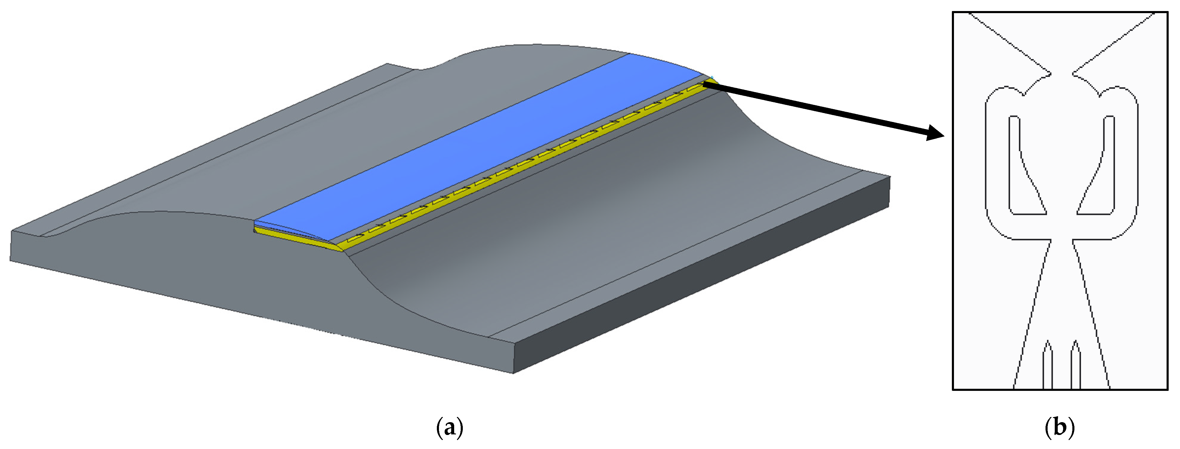
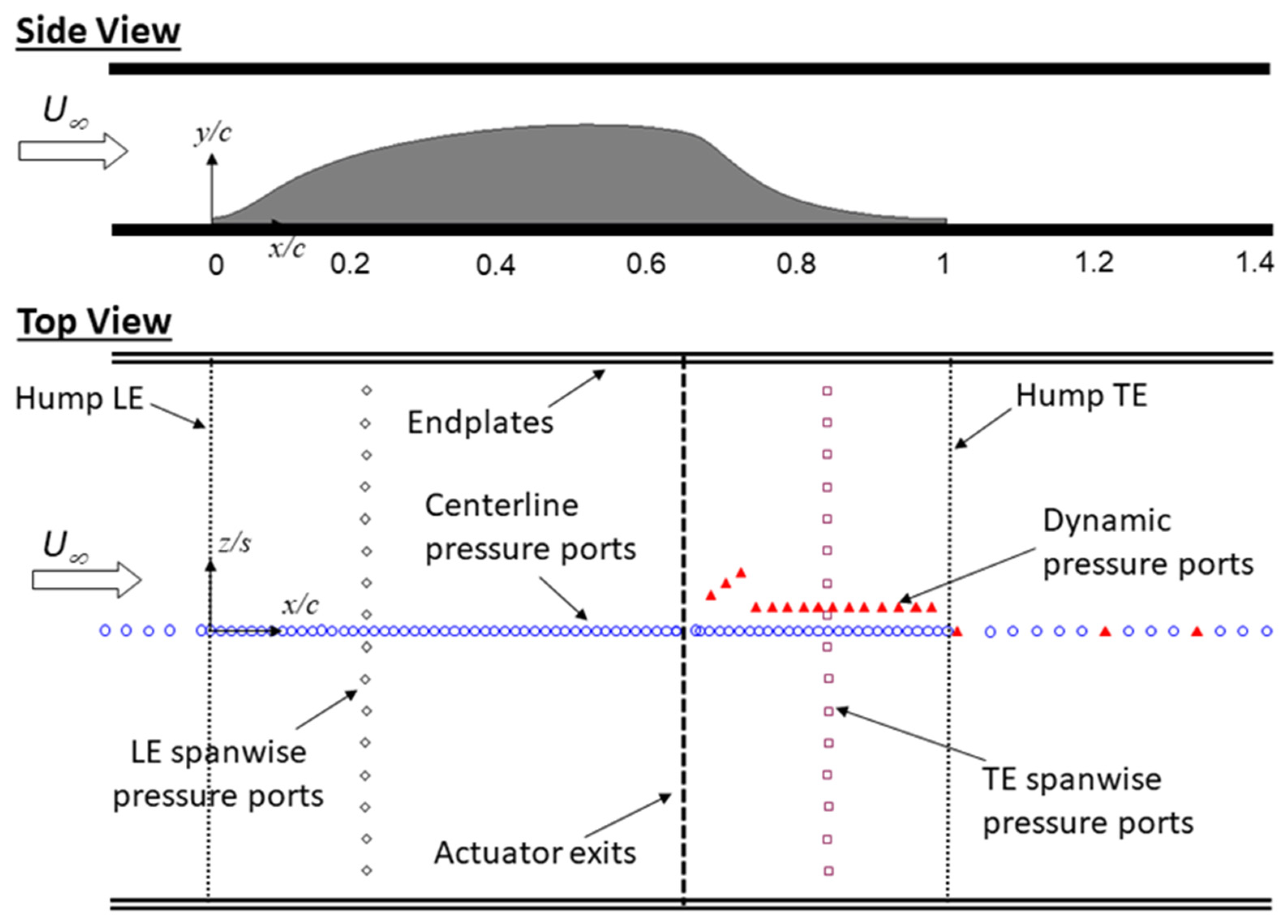
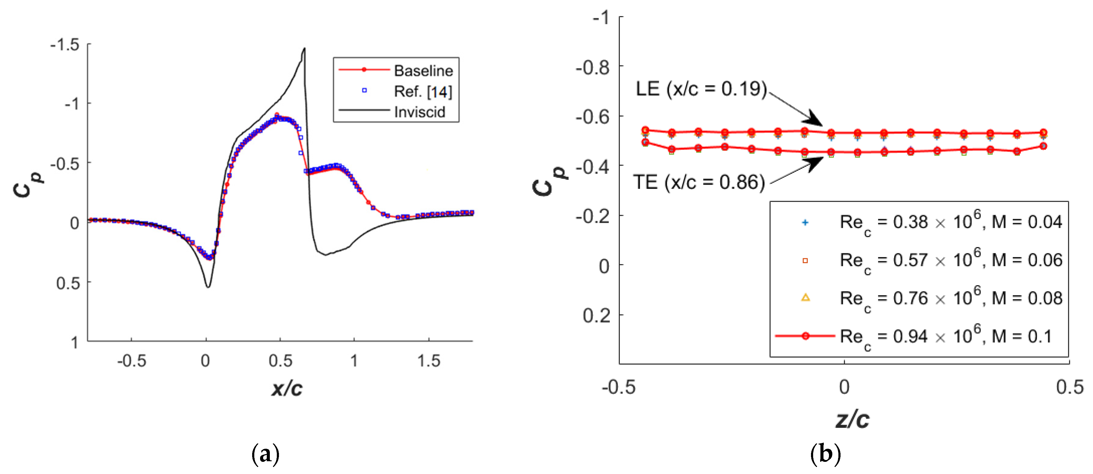
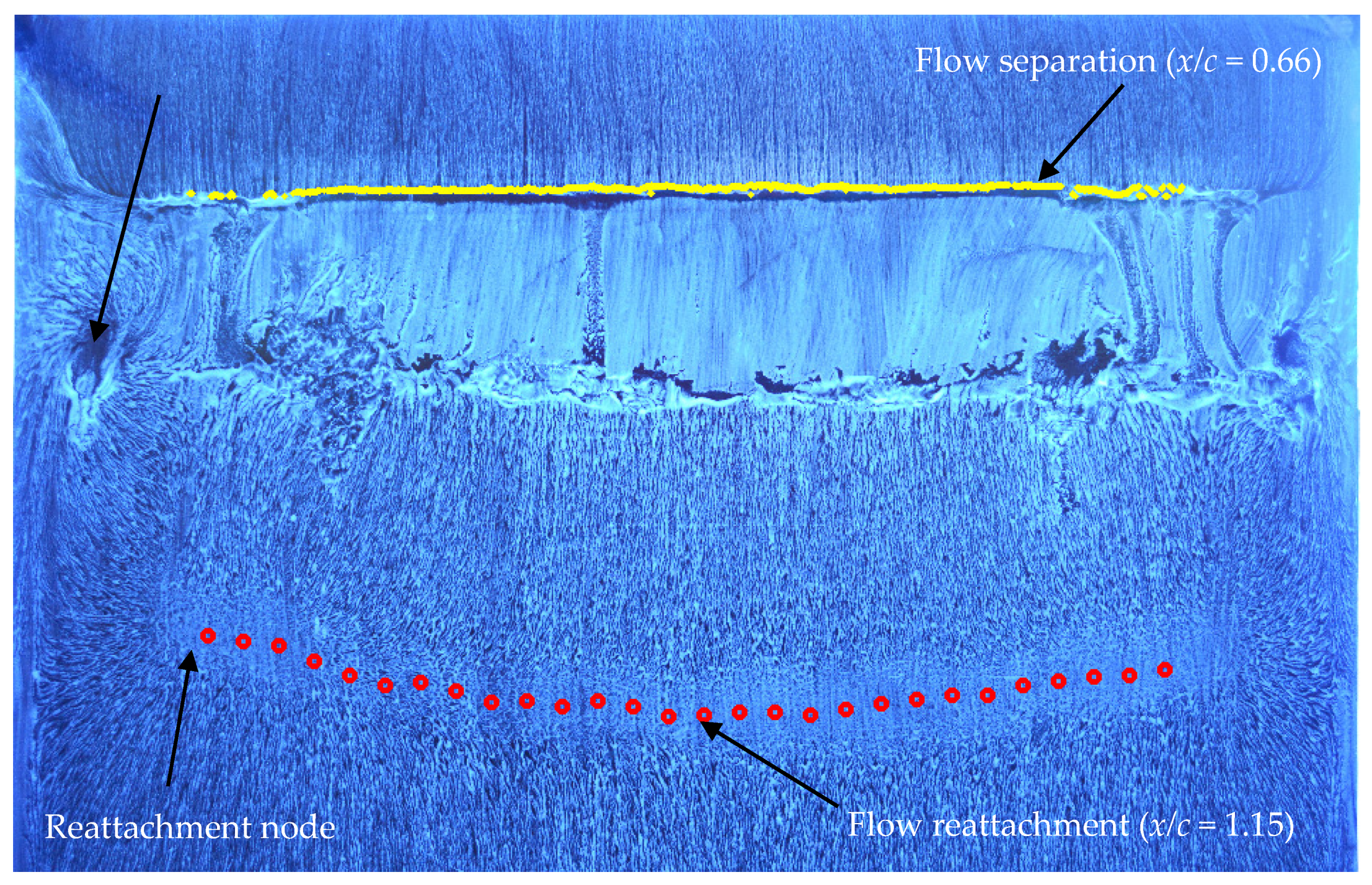
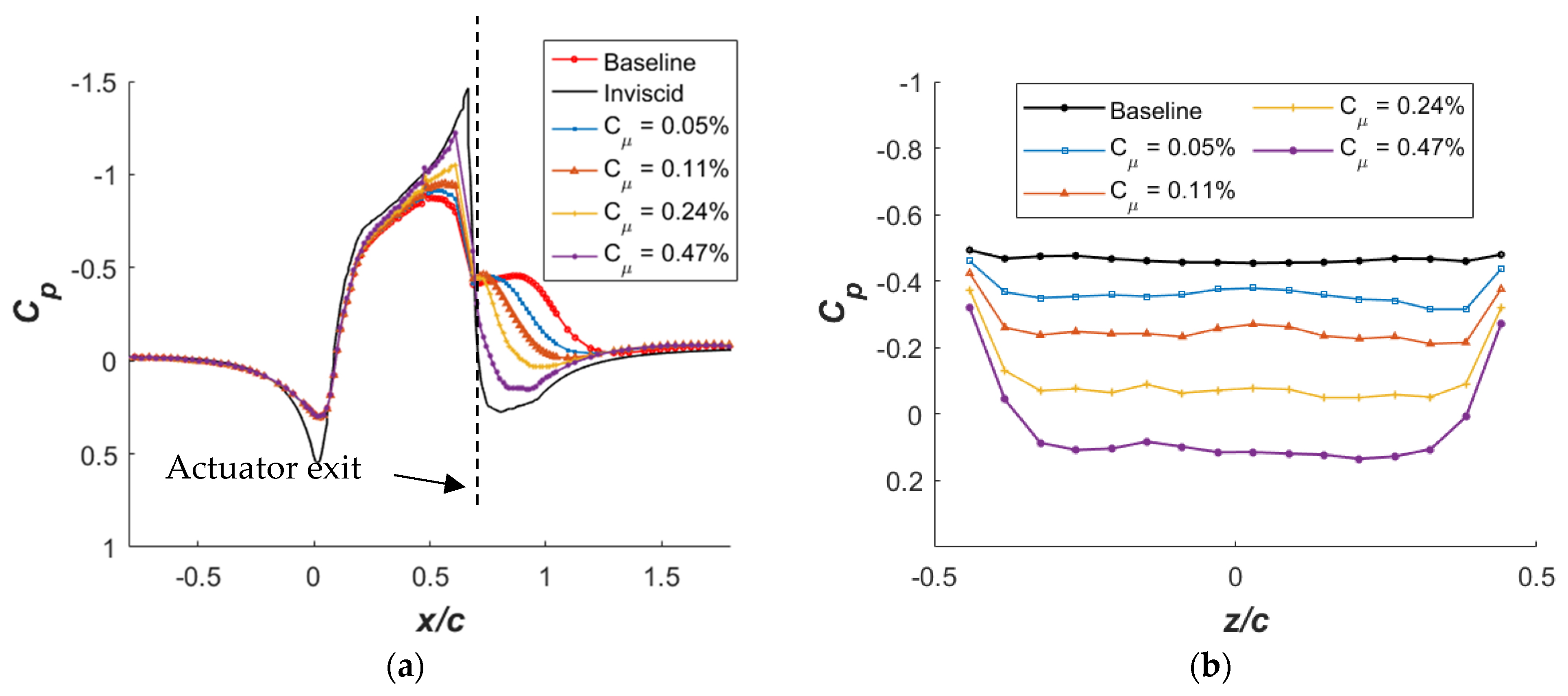
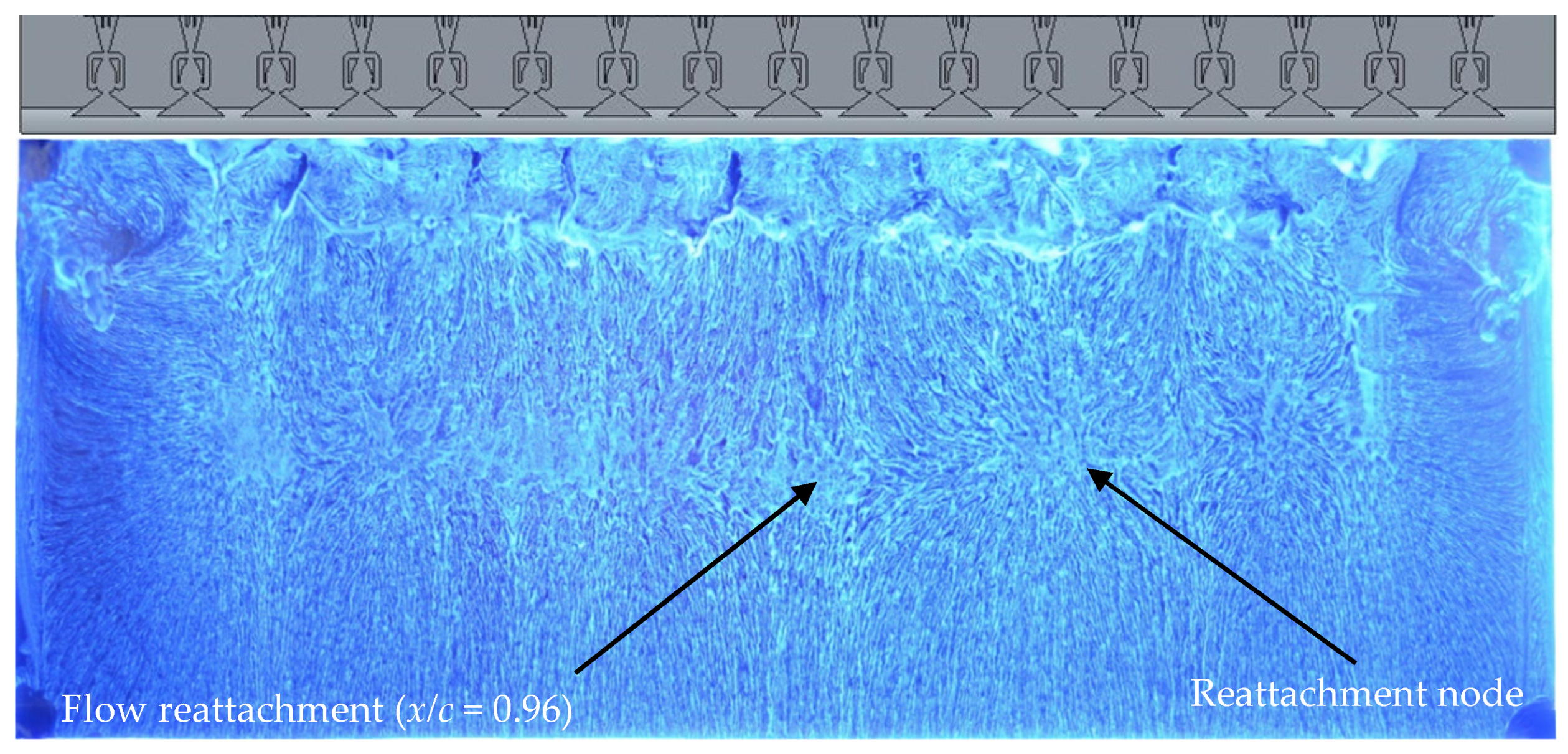
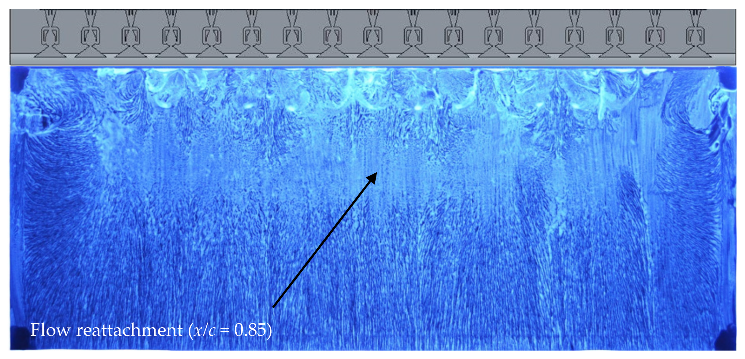
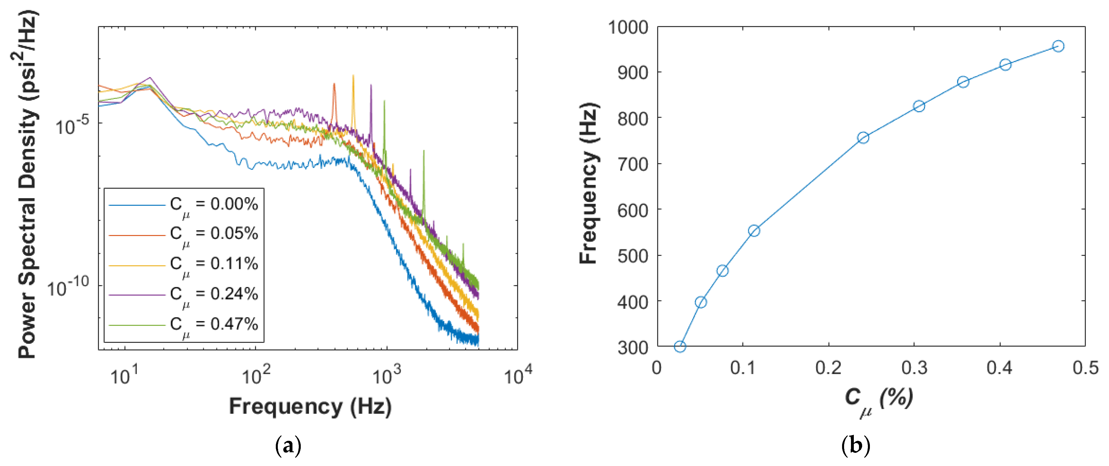
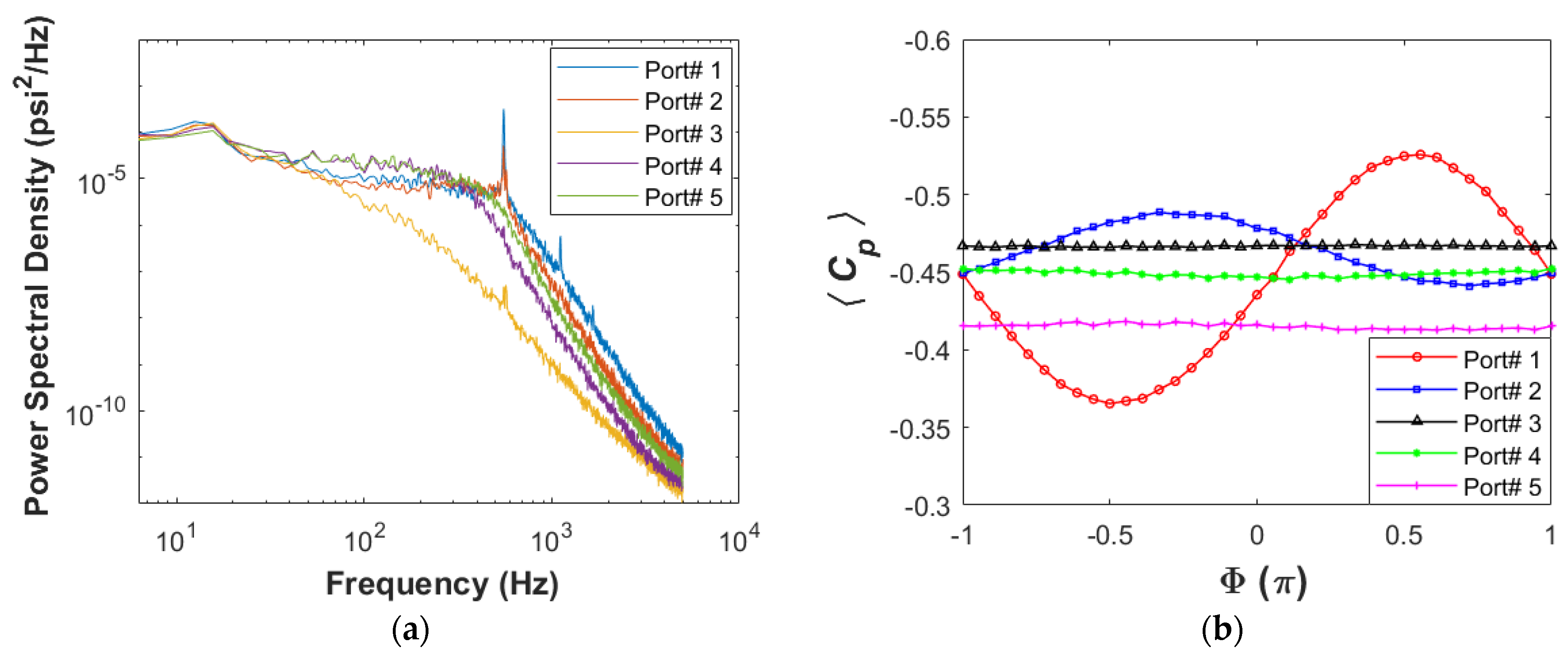
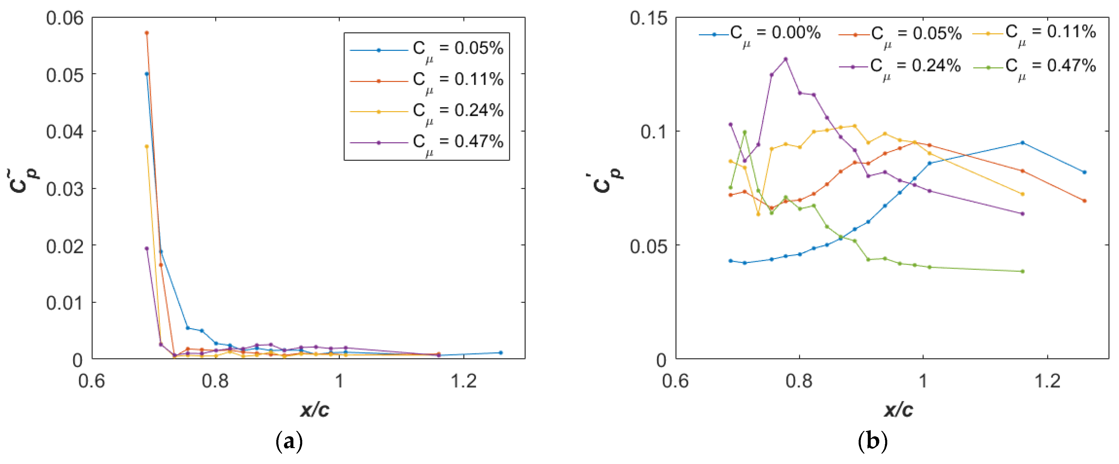
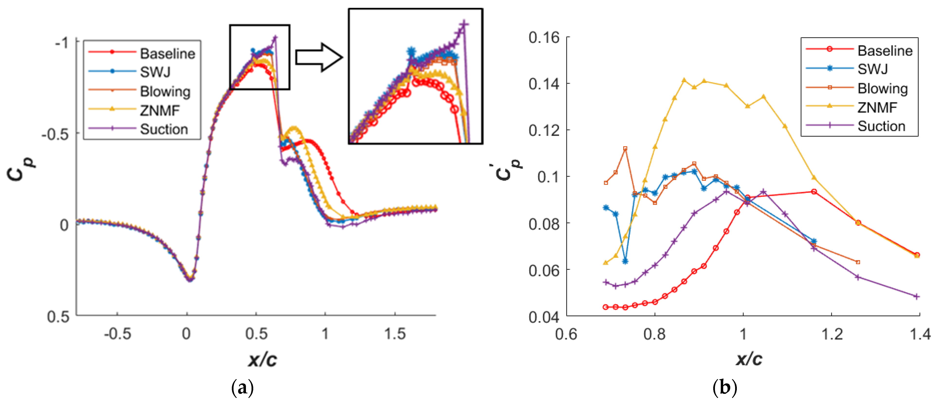
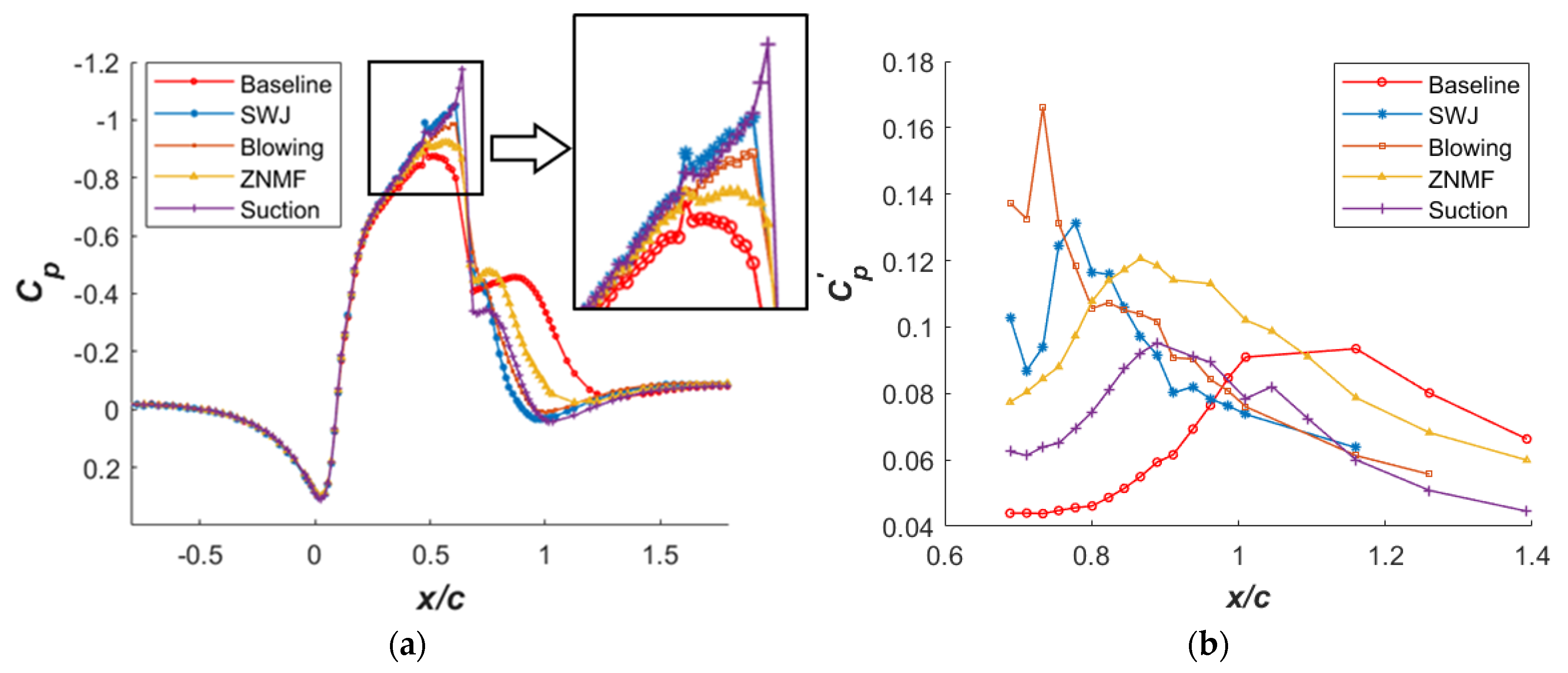
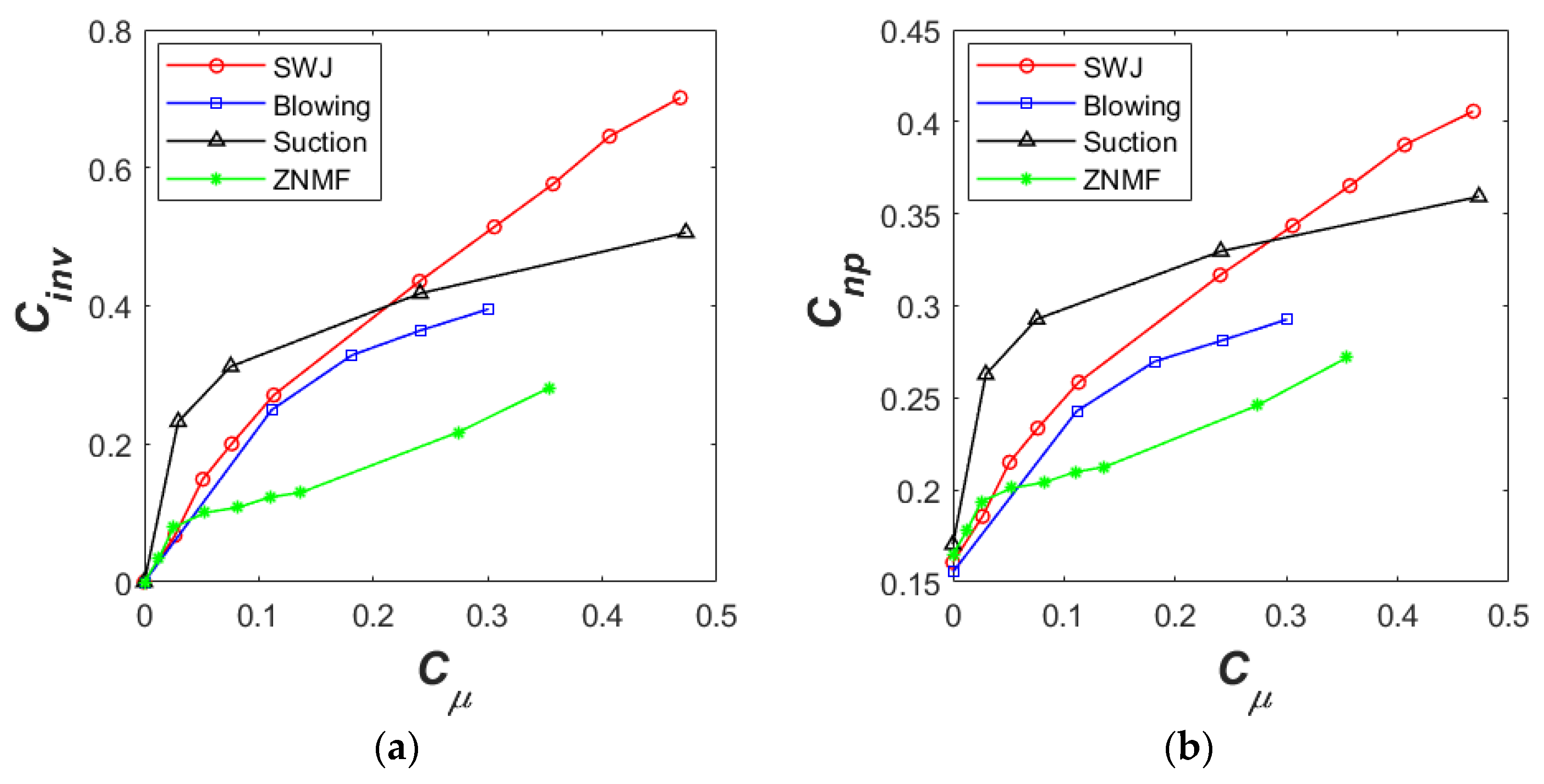
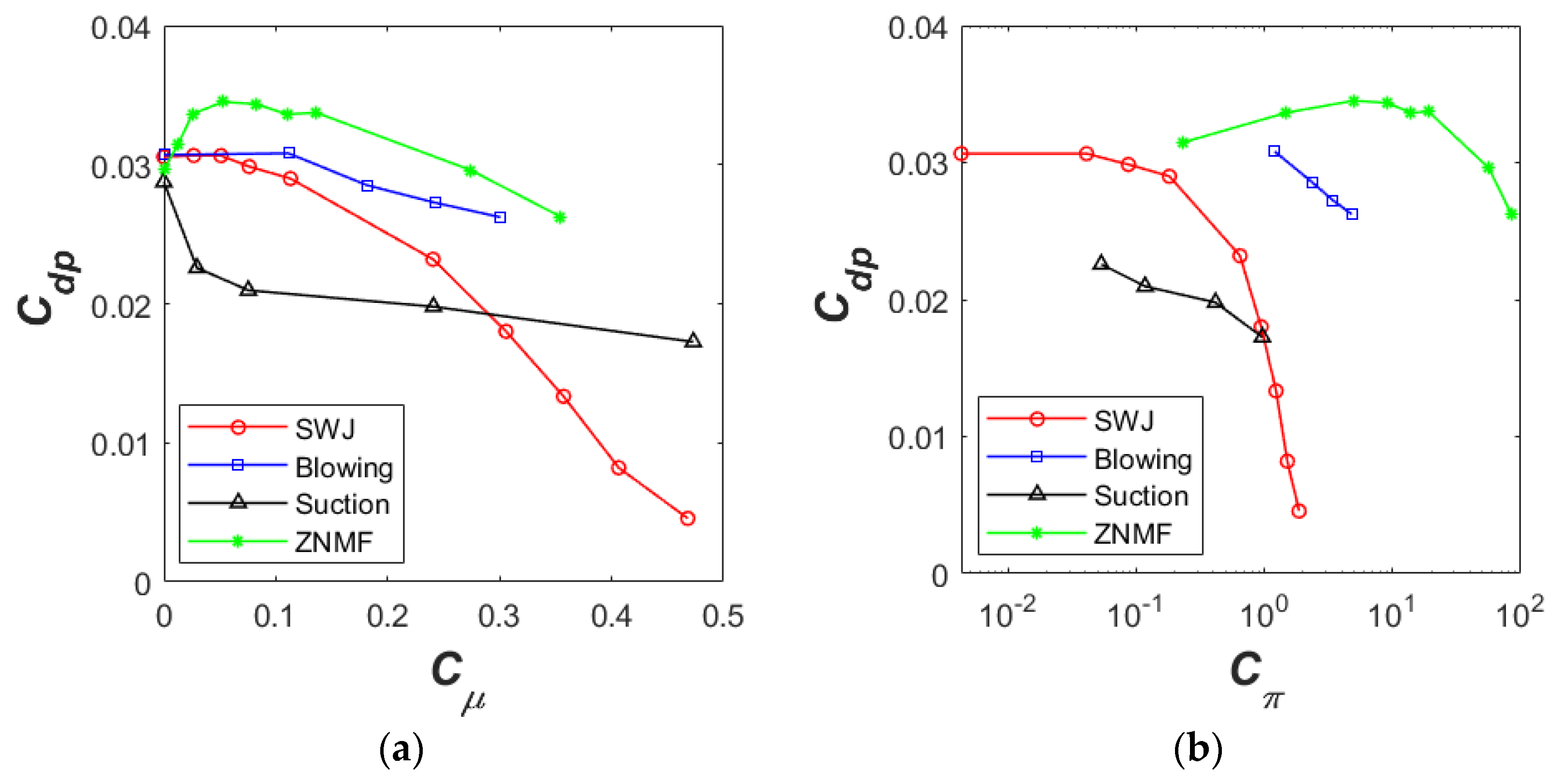
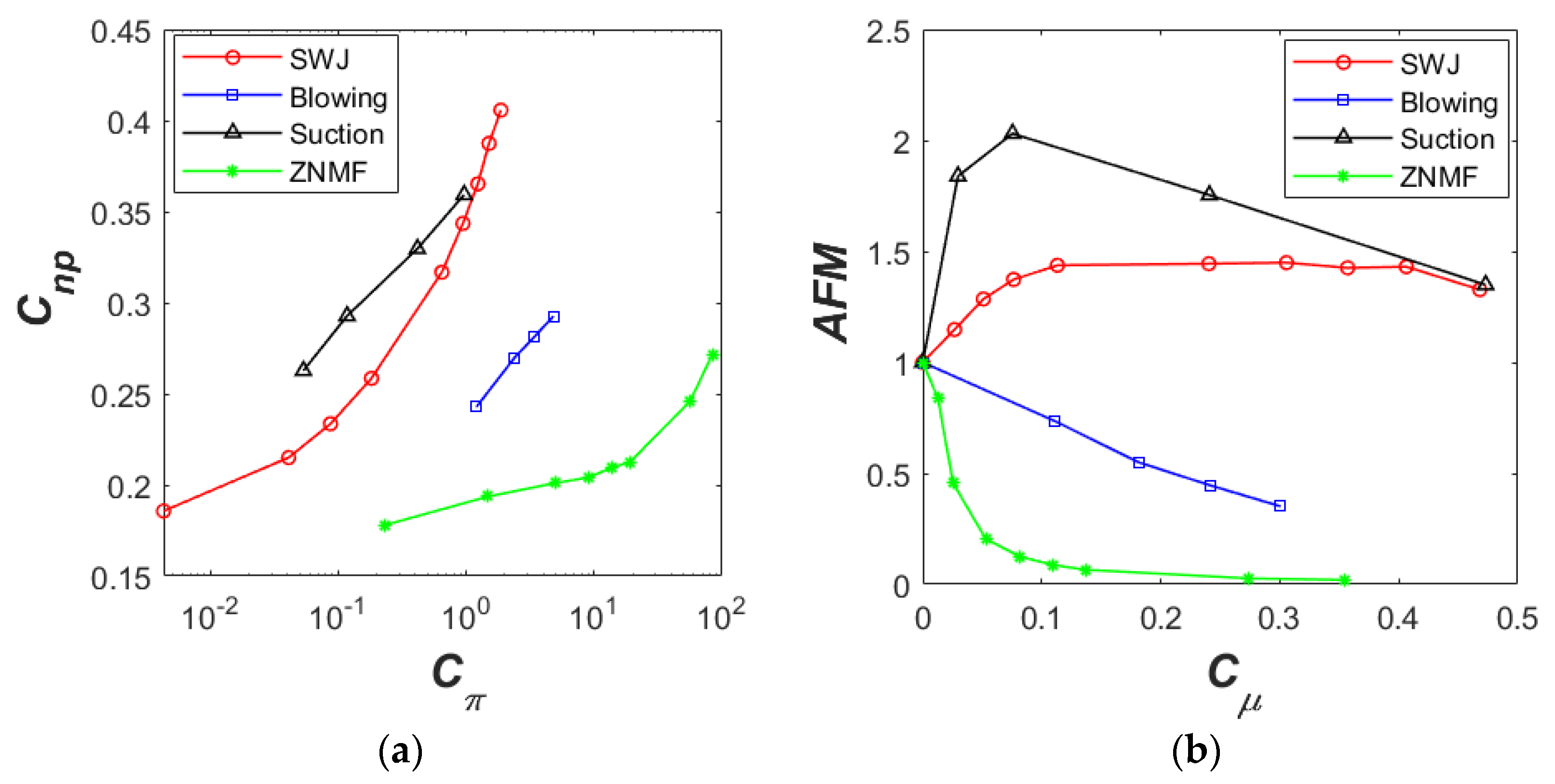
Table 1.
Variation of quality metrics (QM) with momentum coefficient for fluidic oscillators.
| QM | Baseline | Cµ = 0.05% | Cµ = 0.11% | Cµ = 0.24% | Cµ = 0.47% | Inviscid |
|---|---|---|---|---|---|---|
| Cinv | 0.000 | 0.148 | 0.271 | 0.436 | 0.701 | 1.000 |
| Cdp | 0.031 | 0.031 | 0.029 | 0.023 | 0.005 | −0.013 |
| Cnp | 0.161 | 0.215 | 0.258 | 0.317 | 0.406 | 0.506 |
Table 2.
Comparison of quality metrics (QM) for different AFC methods at Cµ = 0.11%.
| QM | Baseline | SWJ | Suction | Blowing | ZNMF | Inviscid |
|---|---|---|---|---|---|---|
| Cinv | 0.000 | 0.271 | 0.312 | 0.249 | 0.123 | 1.000 |
| Cdp | 0.031 | 0.029 | 0.021 | 0.031 | 0.034 | −0.013 |
| Cnp | 0.161 | 0.258 | 0.293 | 0.243 | 0.210 | 0.506 |
Table 3.
Comparison of quality metrics (QM) for different AFC methods at Cµ = 0.24%.
| QM | Baseline | SWJ | Suction | Blowing | ZNMF | Inviscid |
|---|---|---|---|---|---|---|
| Cinv | 0.000 | 0.436 | 0.418 | 0.365 | 0.217 | 1.000 |
| Cdp | 0.031 | 0.023 | 0.020 | 0.027 | 0.030 | −0.013 |
| Cnp | 0.161 | 0.317 | 0.330 | 0.281 | 0.246 | 0.506 |
Publisher’s Note: MDPI stays neutral with regard to jurisdictional claims in published maps and institutional affiliations. |
© 2021 by the author. Licensee MDPI, Basel, Switzerland. This article is an open access article distributed under the terms and conditions of the Creative Commons Attribution (CC BY) license (http://creativecommons.org/licenses/by/4.0/).
Share and Cite
MDPI and ACS Style
Koklu, M. Performance Assessment of Fluidic Oscillators Tested on the NASA Hump Model . Fluids 2021, 6, 74. https://0-doi-org.brum.beds.ac.uk/10.3390/fluids6020074
AMA Style
Koklu M. Performance Assessment of Fluidic Oscillators Tested on the NASA Hump Model . Fluids. 2021; 6(2):74. https://0-doi-org.brum.beds.ac.uk/10.3390/fluids6020074
Chicago/Turabian StyleKoklu, Mehti. 2021. "Performance Assessment of Fluidic Oscillators Tested on the NASA Hump Model " Fluids 6, no. 2: 74. https://0-doi-org.brum.beds.ac.uk/10.3390/fluids6020074