Diesel Migration and Distribution in Capillary Fringe Using Different Spill Volumes via Image Analysis

Abstract

Laboratory-scale column experiments were conducted to assess the impact of different LNAPL volumes on LANPL migration behavior in capillary zone in porous media. Three different volumes of diesel (50 mL, 100 mL, and 150 mL) were released in different experiments using a 1D rectangular column filled with natural sand. The water table was set at 29 cm from the bottom of the column. The image analysis results provided quantitative time-dependent data on the LNAPL distribution through the duration for the experiments. Results demonstrated that the higher diesel volume (150 mL) exhibited the faster LNAPL migration through all experiments. This observation was due to the high volume of diesel as compared to other cases which provides high pressure to migrate deeper in a short time. In all experiments, the diesel migration was fast during the first few minutes of observation and then, the velocity was decreased gradually. This is due to pressure exerted by diesel in order to allow the diesel to percolate through the sand voids. Overall, this study proved that the image analysis can be a good and reliable tool to monitor the LNAPL migration in porous media.

1. Introduction

Organic compound pollution of groundwater and soil in the form of non-aqueous phase liquids (NAPLs) is a widespread environmental problem [1,2]. These pollutants have a negative effect on groundwater quality, rendering it unsuitable for human use and irrigation [3]. Because of their low aqueous solubility, many NAPLs are insoluble in water. As a result, they have the potential to persist for several years, contaminating large parts of groundwater [4]. Because of the complex nature of the water–air–NAPL multiphase system, it is difficult to predict the behavior of NAPLs in porous media, especially in the vadose region. NAPLs are divided into two categories based on their density in relation to water: light non-aqueous phase liquids (LNAPLs) and dense non-aqueous phase liquids (DNAPLs). Chlorinated solvents like tetrachloroethylene and tetrachloroethylene are common examples of DNAPL, while petroleum compounds like benzene, toluene, and xylene (BTEX) are common examples of LNAPL [5,6,7]. LNAPLs migrate downward through unsaturated soil due to gravity when a NAPL is released into the subsurface, leaving small ganglia along their way [8]. Because of the wide density difference between LNAPLs and air, the vadose zone provides little resistance, allowing the LNAPL to enter and accumulate on top of the water table. DNAPLs, on the other hand, will join the saturated zone and continue to migrate downward until they encountered hydraulic or capillary barrier [3]. Understanding the fate and transport of NAPLs in subsurface structures is critical for identifying NAPL source zone geometries as well as designing and evaluating remediation schemes [9,10].

Several studies have shown that NAPL migration in the subsurface is influenced by complex processes that are influenced by a variety of factors, including the NAPL’s viscosity, density, saturation, immiscibility, capillary pressure, wettability, and polar nature, as well as the porous medium’s permeability, porosity, pore size distribution, and surface properties [11,12,13,14].

The rise of water through a soil due to the fluid property known as surface tension is also known as capillarity. Because of the surface tension of pore water acting on the meniscus produced in void spaces between soil particles, pore water pressures are less than atmospheric due to capillarity.

Experiments on the behavior of immiscible fluids in soils have been conducted by a number of researchers [15,16,17,18]. For monitoring fluid properties and movement in soil and groundwater, non-invasive techniques such as gamma ray, X-ray attenuation, and electrical conductivity probes have been used [19,20]. Although these studies have provided useful information on the fate and transport of NAPLs in porous media, they have some drawbacks, the most notable of which is that they do not allow for the observation of fluid migration under dynamic conditions and across the entire domain of interest [2,7]. Image analysis approaches such as light propagation visualization, light reflection method, spectral image analysis method, and simplified image analysis method (SIAM) have gained more attention from researchers because of the limitations [16,18,21].

As previously mentioned, NAPLs released into the subsurface environment will last for a very long time. Though capillary forces may keep the NAPL entrapped in the soil, it may undergo some redistribution that affects its fate and transport. In the vadose zone, water percolation into the subsurface can influence the migration of entrapped NAPL ganglia as well as the NAPL mass accumulated on the water table. Alazaiza et al. [14] conducted a 2-D experimental study to observe the influence of rainfall on the migration of LNAPL in double-porosity soil structure. The authors reported that water table fluctuations caused the LNAPL that was entrapped in the porous media to be pushed further downward. In addition, they observed that the capillary fringe thickness was depressed due to the influence of both infiltration and LNAPL volume. Alazaiza et al. [18] applied the simplified image analysis method (SIAM) to investigate the saturation distributions of the LNAPL and water in the entire domain the influence of water table fluctuations. The authors concluded that the SIAM technique is an accurate and cost-effective tool for the visualization of the time-dependent NAPL/water movement in laboratory-scale experiments and quantifying dynamic changes in fluid saturation in porous media.

The present study aims to investigate the influence of LNAPL spill volume on the migration behavior in porous media. Specifically, SIAM is applied to produce detailed time-dependent LNAPL migration in a 1-D sand column. Diesel was used as a representative of LNAPL, and the sand used was a natural river sand.

2. Materials and Methods

2.1. Materials Characteristics

A natural sand collected from a river was used as a porous media. General characterization was conducted to investigate the main properties of the sand prior to experiments. Particle size analysis indicated that the pore grain size varied between 0.4 mm and 1.22 mm with an average size of 0.71 mm. The basic physical characteristics of the sand are presented in

Table 1. The basic physical properties of sand.

Parameter	Test	Value
Coefficient of permeability (m/s)	Constant head permeability	4 × 10−10
Average diameter (mm)	Sieve analysis	0.30
Coefficient of uniformity, Cu		2.19
Density (g/cm3)	Small pyknometer	2.66
Porosity	Calculated	0.40

. LNAPL was represented using a commercial diesel fuel with a density of 0.83 g/cm³ and a viscosity at 20 °C of 5.8 mm²/s. The thermal expansion coefficient was 88 kg/m³, flash point at 62 °C, and vapor pressure was 10 kPa at 15 °C [22]. The LNAPL was mixed with Red Sudan III dye while water was dyed using a Brilliant Blue FCF dye with 0.1% of volume to enhance the visualization.

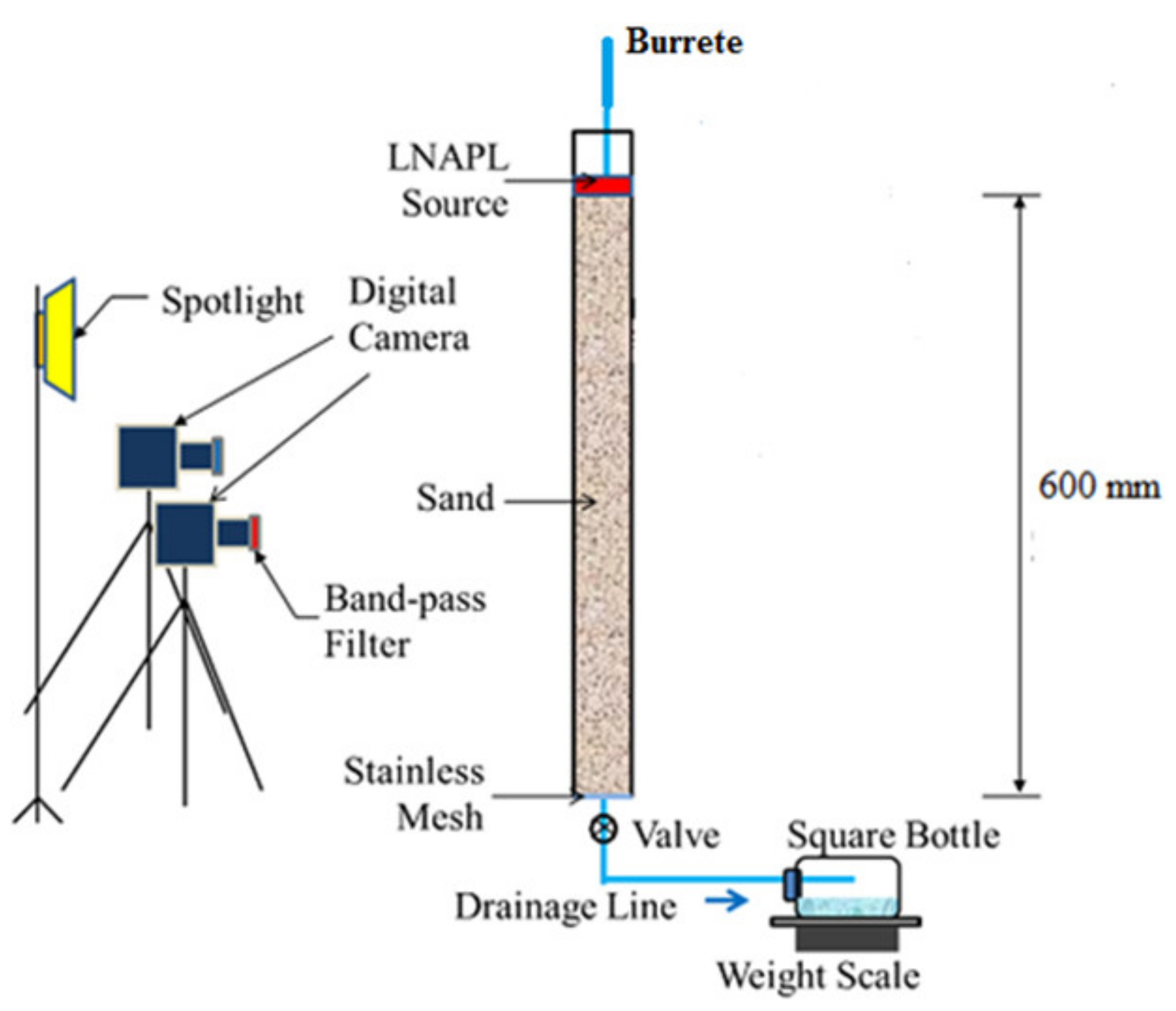
2.2. Experimental Setup

For all experiments, a 1-D square acrylic glass column with dimensions of 30 mm width × 30 mm depth × 500 mm height and a 10 mm thick wall was used. The acrylic glass was translucent so that fluid migration within the sand column could be observed. Transparent glue was used to stack the column joints together. Two digital cameras (Nikon D5100 and Nikon D5300) were mounted 1 m in front of the column with two separate narrow bandpass filters (BN-650 and BN-470) attached to capture images during the experiments. In the column test, the BN-650 bandpass filter was used to assess the light intensity of the diesel, while the BN-470 bandpass filter was used to detect the light intensity of the water. In addition, two LED floodlights were installed as the primary source of illumination in the dark space. As a white color guide, a GretaMacbeth white balance board was fixed beside the column. To avoid displacement and vibration during image processing, a Nikon Camera Control Pro Software was used to capture images automatically. Manual changes were made to the camera settings to improve the dynamic range of the cameras by using exposure times of just a few seconds. The aperture of the lenses used was set at f-16 for all photographs, and the exposure time was 2.5 s, yielding a resolution of f/16 (0.030 by 0.035 cm²). According to the procedure defined by Bob et al. [16], the temporal variation in light intensity was corrected. A reference image was produced that reflected the image captured when the column was fully saturated with water. On the reference image, two small squares (2 cm × 2 cm) were identified as “correction zones”.

The correction coefficients were determined using the ratio of the reference image’s average light intensity of the correction zones to the image’s average light intensity of the correction zones that needed to be processed. To correct a particular image, for example, the correction coefficient of the image to be corrected was multiplied by the image’s light intensities. Three subsequent images were taken for each image, and the average value of the light intensities of these three images was used in the calculations. MATLAB was used to analyze all the images. All tests were carried out in duplicate inside a dark room that was held at a temperature of 23 ± 1 °C. Figure 1 portrays the experimental setup.

2.3. Experimental Procedure

Before starting the experiments, the sand was washed with distilled water to eliminate any fine residuals and then oven dried for 48 h at 45 °C to remove any moisture [15,23]. Following that, the sand was gradually packed into the column in 2 cm layers. The sand column was fixed on a mechanical vibrator with a vibration rate of 50 hertz to ensure uniform compaction and identical void ratios in all column experiments. It was found that the porosity of the sand was 0.39, which is equal to a pore volume of 295 mL. After that, the sand was saturated with blue-dyed water and put in a vacuum chamber for 24 h to eliminate any trapped air and ensure that the sand was fully saturated with water. The drainage valve was then opened to drain the water into the tank, resulting in the water table being set at 29 cm from the column’s bottom. Three different diesel volumes were used to investigate the effect of different diesel spill volumes on LNAPL migration in sand column. These volumes were 50 mL, 100 mL, and 150 mL. Digital cameras were set to capture an image each 1 min in order to monitor the changes in diesel behavior.

2.4. Simplified Image Analysis

The definition of NAPL zones needs precise NAPL saturation measurements. Additionally, in controlled laboratory environments, collecting precise quantitative data on saturation is a difficult task. Since soil samples must be separated from a soil sample, the gravimetric sampling process, though reliable, cannot provide continuous saturation data. Furthermore, sampling only offers information from one or a few chosen locations. Alazaiza et al. [18] developed the SIAM to observe the saturation distributions of LNAPL and water in the partially saturated sand column under complex conditions in this study. The SIAM’s theory is based on the Beer-Lambert law of light transmittance, which assumes a linear relationship between the average optical density, LNAPL, and water saturation (S_o and S_w, respectively). The following formula can be used to measure the average optical density:

$${\mathrm{D}}_{\mathrm{i}}=\frac{1}{\mathrm{N}}{\displaystyle \sum _{\mathrm{j}=1}^{\mathrm{N}}{\mathrm{d}}_{\mathrm{j}\mathrm{i}}=\frac{1}{\mathrm{N}}{\displaystyle \sum _{\mathrm{j}=1}^{\mathrm{N}}\left[-{\log }_{10}\left(\frac{{\mathrm{I}}_{\mathrm{j}\mathrm{i}}^{\mathrm{r}}}{{\mathrm{I}}_{\mathrm{j}\mathrm{i}}^{\mathrm{o}}}\right)\right]}}$$

(1)

where D_i is the average optical density, i is the spectral band (i = 470 or 650), N is the number of pixels in the area of interest, d_ji is the optical density of the individual pixels, I^r_ji is the light intensity of the reflected light by individual pixel value, and I⁰_ji is the light intensity of the reflected light by an ideal white surface.

From the calculated D_i, SIAM can estimate the saturation distribution matrices [S_w] and [S_o] by performing a comparison between the average optical densities of the matrix element (Di) and the three calibrated images (D^w_i, D⁰_i, D^d_i) for sand fully saturated with water (S_w = 100%, S_o = 0%), sand fully saturated with LNAPL (S_w = 0%, S_o = 100%), and dry sand (S_w = 0%, S_o = 0%), respectively, for the same range. The average optical density values for each cell of the studied range can be calculated and compared to the corresponding ones for all three calibration images. A matrix of correlation equation sets can also be obtained, with each one corresponding to each cell as follows:

$${\left[\begin{array}{l}\mathrm{D}\mathrm{i}\\ \mathrm{D}\mathrm{j}\end{array}\right]}_{\mathrm{m}\mathrm{n}}={\left[\begin{array}{l}({\mathrm{D}}_{\mathrm{i}}^{\mathrm{w}}-{\mathrm{D}}_{\mathrm{i}}^{\mathrm{d}}){\mathrm{S}}_{\mathrm{w}}+({\mathrm{D}}_{\mathrm{i}}^{\mathrm{o}}-{\mathrm{D}}_{\mathrm{i}}^{\mathrm{d}}){\mathrm{S}}_{\mathrm{o}}+{\mathrm{D}}_{\mathrm{i}}^{\mathrm{d}}\\ ({\mathrm{D}}_{\mathrm{j}}^{\mathrm{w}}-{\mathrm{D}}_{\mathrm{j}}^{\mathrm{d}}){\mathrm{S}}_{\mathrm{w}}+({\mathrm{D}}_{\mathrm{j}}^0-{\mathrm{D}}_{\mathrm{j}}^{\mathrm{d}}){\mathrm{S}}_{\mathrm{o}}+{\mathrm{D}}_{\mathrm{j}}^{\mathrm{d}}\end{array}\right]}_{\mathrm{m}\mathrm{n}}$$

(2)

where m and n are matrix dimensions, [D_i]_mn and [D_j]_mn are the average values of the optical density of each mesh element for wavelengths i and j, [D_di]_mn and [D_dj]_mn are the average optical density of each mesh element for dry sand; [D_wi]_mn and [D_wj]_mn are for water saturated sand; and [D_oi]_mn and [D_oj]_mn are for LNAPL saturated sand. Equation (2) is essentially an averaging of the optical density of the three fluids (water, LNAPL, and air), each weighted by its saturation.

3. Results and Discussion

3.1. Determination of Capillary Height

The capillary height (h_c) was determined by adjusting the water table from the water reservoir to a specific desired height. After the sand was placed in the column, the drainage valve was opened instantly. The water capillarity monitoring was left for 24 h. After 24 h, the capillary height value observed was around 28 cm. Because of the small void spaces between sand particles, the rising value of h_c means that water capillarity in sand moves upwards at a faster rate. According to Liu et al. [24], several soil parameters such as effective grain size, void ratio value, and pore size distribution are the key considerations in determining the maximum height of capillary rise in soils. As a result, any changes in the specified soil properties can change the capillary height. Day [25] also concluded that the interactions between pore water pressure and atmospheric pressure play an important role in determining the capillary rise in soil caused by pore spaces in soil particles. Based on Terzaghi and Peck [26], the height of capillary can be estimated from the equations below:

H_c,max = C/eD₁₀

(3)

e = G_s γ_w/γ_d

(4)

γ_d = W/V

(5)

where C is the grain shape constant of sand which is in the range of 10 to 50 mm² [26]. D₁₀ is the effective grain diameter obtained from soil classification. e: is the void ratio.

Equation (4) is used to calculate the void ratio where:

• G_s is specific gravity of soil
• γ_w is the unit weight of water in the soil
• γ_d is unit weight of dry soil
• W is the mass of the dry soil
• and V is the volume of the dry soil.

Equation (3) is used to calculate the dry unit weight of soil. The total dry sand used in the column was 1100 g, thus, the dry unit weight calculated according to Equation (5) was 15.7 kN/m³. The void ratio obtained using Equation (2) was 0.69. By substituting Equations (3) and (4) into Equation (5), the capillary height, h_c obtained was between 280 mm and 314 mm according to the value of C. The difference of h_c value is due to some parameters provided from both equations are different. According to Liu et al. [24] in determining maximum capillary rise height in a short period of time, the parameters which is contact angle, dry density, specific gravity, pore space, and hydraulic properties can be applied.

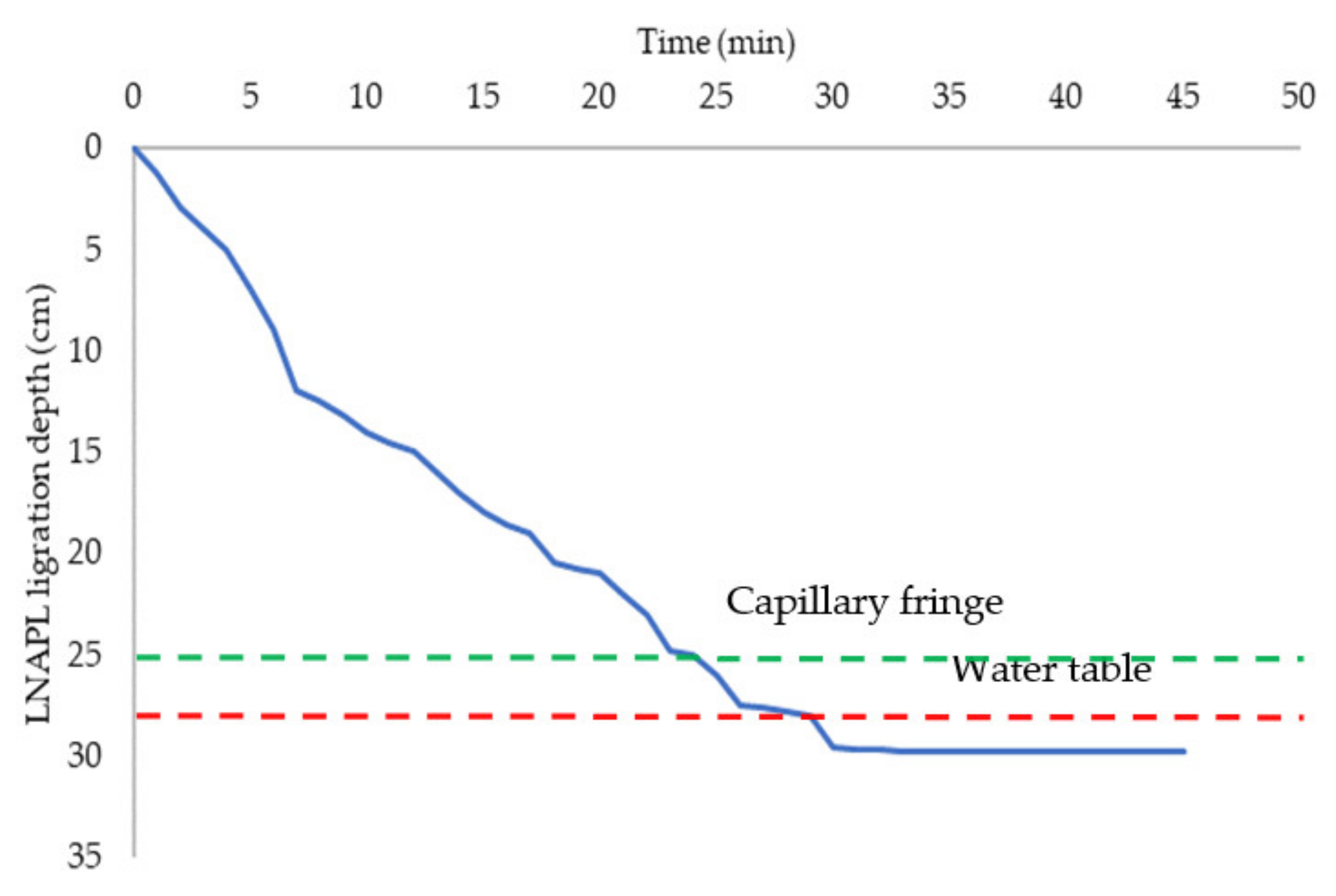
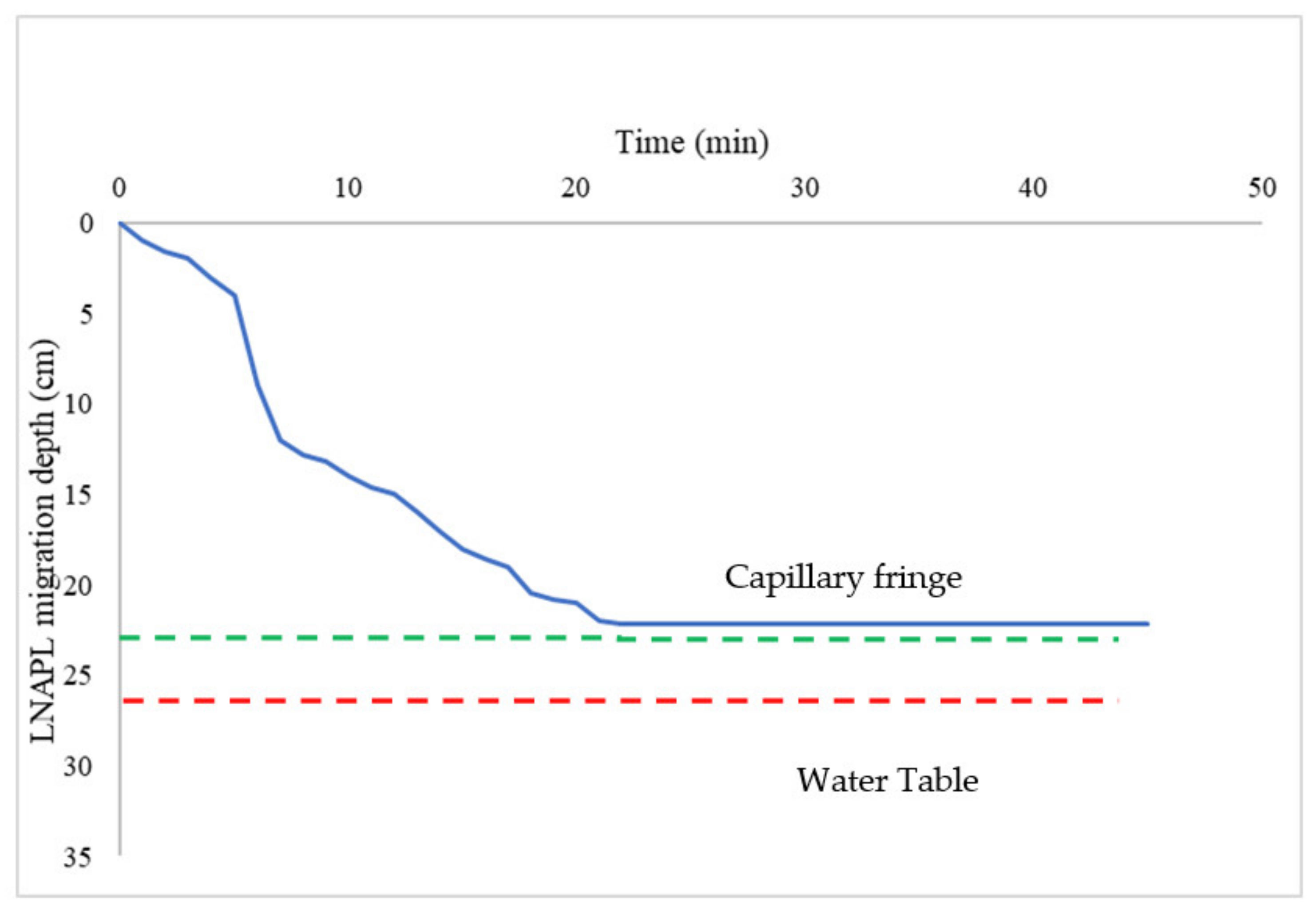
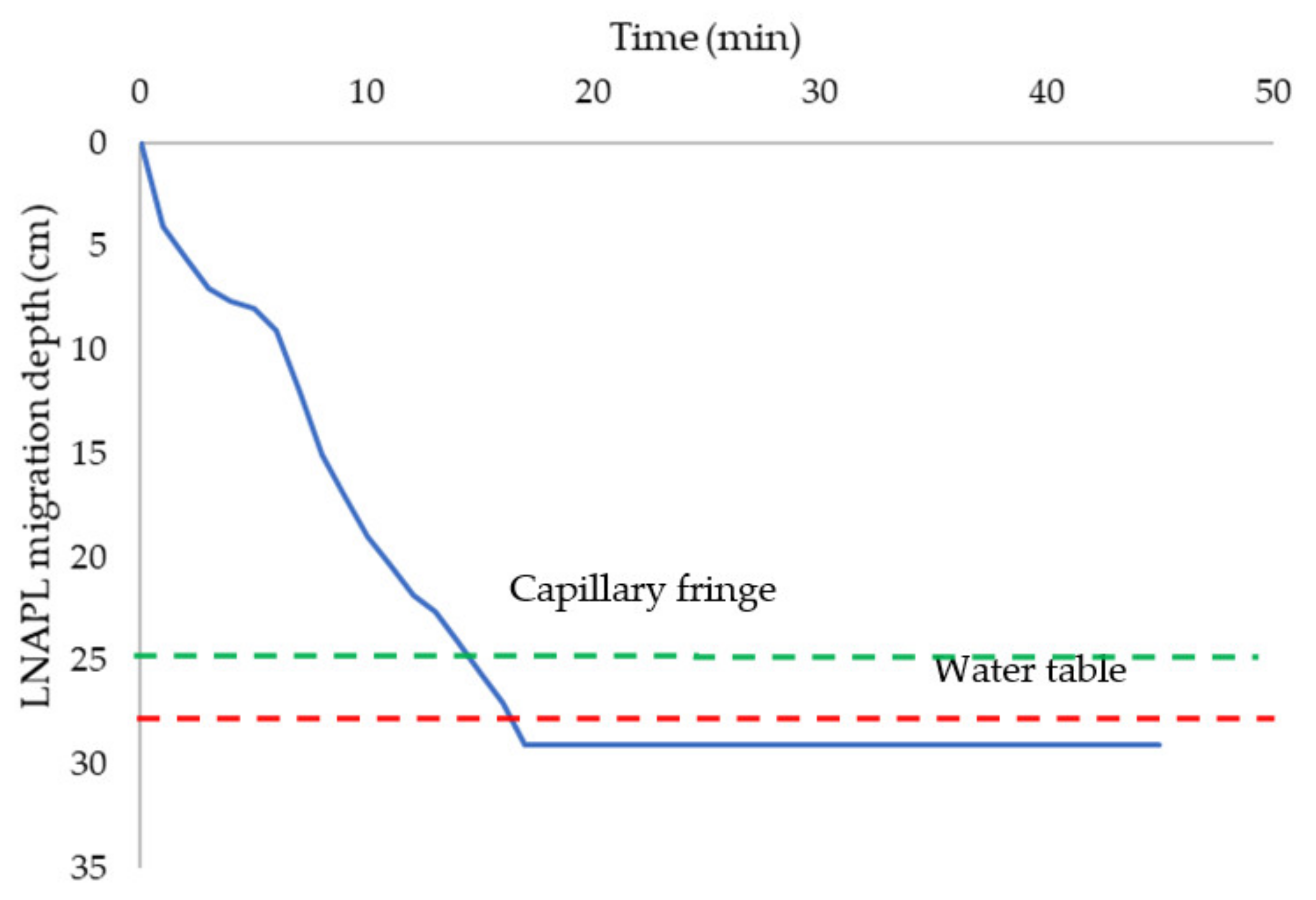
3.2. Effect of Diesel Spill Volume

Due to many factors, including entrapment of LNAPL at residual saturations and viscosity rate of LNAPLs, determining the exact amount of LNAPL spills under a leaking underground storage tank (LUST) is difficult. When LNAPL is removed, water invades the void space, causing LNAPL flow paths to become narrower, reducing the porous media’s ability to allow LNAPL migration. As the LNAPL becomes immobile due to saturation, the reduced size of flow paths in porous media causes the large LNAPL spill volume to become more complicated. As a result, as the saturation of LNAPL increases, the recovery rate process becomes more difficult. Using Equation (2) and substituting with the values of the unit weight of water, γ_w, maximum dry density, γ_d, and specific gravity, G_s, the diesel spill volume needed to contaminate the sand particles can be determined based on the observation of the column test. The porosity value, n, needed to enable the diesel to fill the pore spaces can be calculated using the calculated void ratio, e, obtained from these parameters.

n = e/(1 + e)

(6)

The volume of void in the sand is equal to the total volume of diesel required to fill the void spaces of sand particles and contaminate it. The calculated porosity was 0.40 which resulted in a volume of diesel required to contaminate the sand particles with a value of is 0.00029 m³. As a result, if the sand column is set up with different dimensions, the appropriate diesel spill volume would be different as well, due to the different void ratio and porosity values. The propensity of diesel to hit the ground water table was faster when enough diesel volume was released and flowed downward through the sand column. Because of the high volume and weight of the migrated diesel, it exerted a high pressure on the sand, allowing it to be polluted at a faster rate. The diesel will begin to fill the void spaces in the sand particles as it migrates downwards under the effect of gravity. Diesel displaced blue dye solution from the interior of the largest pores during this process. The ability of diesel to displace dye solution from larger pores than smaller pores has been demonstrated by selective entry of diesel into larger voids. More diesel would be displaced, resulting in a larger network of interconnected pores containing diesel. According to Simantiraki et al. [27], diesel spreads faster in the vertical direction in fine sand because fine sand particles have smaller void spaces, resulting in higher capillary pressure.

3.3. Diesel Migration Influence on Capillary Height

The volume of LNAPL spills is one of the most important factors that can influence the severity of pollution of the subsurface. Several researchers reported that even small amounts of LNAPLs spilled could seriously contaminate ground water [28]. In this study, three different volume of diesel was used as mentioned earlier. In prior to spilling the diesel, the capillary fringe height was left for 24 h. Within 24 h, saturated capillary fringe could move upwards to 28 cm from the water table and leave only 2 cm of the vadose zone. The total period to conduct this experiment was set to 2.5 h. Within this period, the volume of diesel had completely migrated downward through the sand particles. The elevation change of capillary height was also observed during the whole experiment. After 2.5 h, no change of elevation for capillary height or capillary fringe zone was observed due to diesel migration. From the visual observation, no capillary action was observed including the capillary depression in the capillary fringe zone, despite different volumes of spilled diesel used. As a result, the volume and weight of spilled diesel can be increased, putting more pressure on the diesel, and allowing it to infiltrate the capillary fringe zone.

The density of the sand in the column also plays a significant role in determining capillary rise. The porosity and void ratio of the sand particles decreased as they were compacted, resulting in smaller void spaces in the sand particles. The density of sand is constant in the study of diesel migration behavior since the weight and volume of sand used in the study are constant. Owing to gravitational force, capillary force, and viscosity factor, diesel is less dense than water, thus it migrates downward. When a large amount of diesel is spilled, the propensity for the diesel to fill up the sand void space becomes easier, compared to when a small volume of diesel is spilled, since the volume spill exerts more pressure. Figure 2 shows the migration of the 50 mL diesel volume in the sand column.

As shown in Figure 2, the diesel migrated very fast during the first 10 min. This is due to pressure exerted by diesel in order to allow the diesel to percolate through the sand voids. After that, diesel continued its migration but with a less velocity compared to the first 10 min. After 30 min of migration, diesel velocity started to be constant and no obvious change in the velocity was observed. Diesel reached the bottom of the column after 30 min. This could be because the 50 mL of diesel spilled does not fill up all the void spaces of sand particles. Another reason is that the diesel tends to migrate and find the lowest point, as the sand may not well-compacted.

For the case of 100 mL diesel volume, diesel took longer to fill the voids and cover the sand particles in the saturated capillary fringe zone, taking more than 22 min. Furthermore, the diesel took longer to reach the ground water level. This may be explained by the fact that diesel appears to accumulate and form a plume before migrating deeper. In addition, it seems that some parts of the NAPL migrated horizontally during the start time of NAPL pouring until it filled the pores around the spillage point. After that, it started to migrate downward.

The pressure of water in the capillary fringe zone allows the diesel to accumulate. As a result, diesel attempts to conquer the water–capillary pressure and migrate lower. The increased diesel plume in the void spaces allowed for more pressure to be applied to penetrate this LNAPL. Figure 3 represents the flow of 100 mL diesel volume within the first 45 min.

For the case of 150 mL, Figure 4 shows that for the first 30 min, 150 mL of diesel spilled has a greater effect on migration depth. The large amount of diesel spilled provides higher pressure to push the migration of LNAPL in faster rate as compared to the cases of 50 mL and 100 mL diesel volume. In addition, the diesel took around 15 min to fill void spaces in the saturated capillary fringe zone. The diesel migrated deeper after 15 min, contaminating the ground water table and sand. Several factors such as soil hydraulic conductivity can also influence the LNAPL spills. This could be explained as the sand has medium degree of permeability which possess good drainage system. Good drainage paths result in a lower resistance to fluid flow. Although the volume and weight of diesel spilled is high, the permeability coefficient can be low as the diesel tends to accumulate and form contamination plume in subsurface environment.

Based on the figures provided above, it can be summarized that the greater the volume diesel spilled, the deeper the migration depth through the subsurface of sand with short time. The 150 mL of diesel portrayed great impact on the sand particles. Due to the good drainage paths of the sand, the infiltrated 150 mL diesel can migrate deeper provided with high pressure subjected to the sand due to the high-volume diesel spilled. Besides, it also required shorter time to fill up the void spaces in the saturated capillary fringe zone which is only 20 min. With high volume of spill, the migration of diesel became continuous due to constant pressure exerted. Hence, this will induce more constant rate of the 150 mL diesel infiltration as compared to 50 mL and 100 mL of diesel volumes. Figure 5 showed the images of the different volumes of diesel in the sand column. It is worth mentioning that in real life and real application, the diesel plume shape as well as velocity could be different from the results shown in this study. This is because of the column wall on the migration of fluids. The wall effect is very common in 2-D columns and results in looser packing along the column wall compared to the rest of the column parts.

4. Conclusions

• Three 1-D laboratory experiments were carried out to investigate the effect of different LANPL volumes on its migration through sand column using simplified image analysis method.
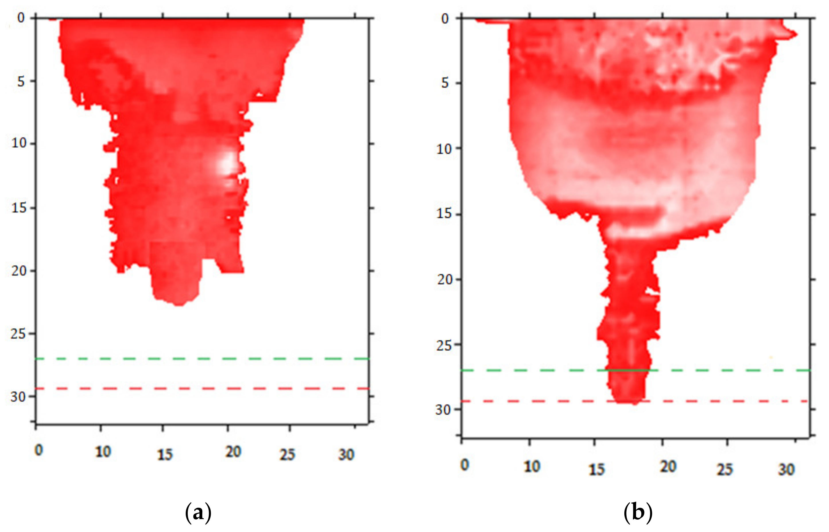
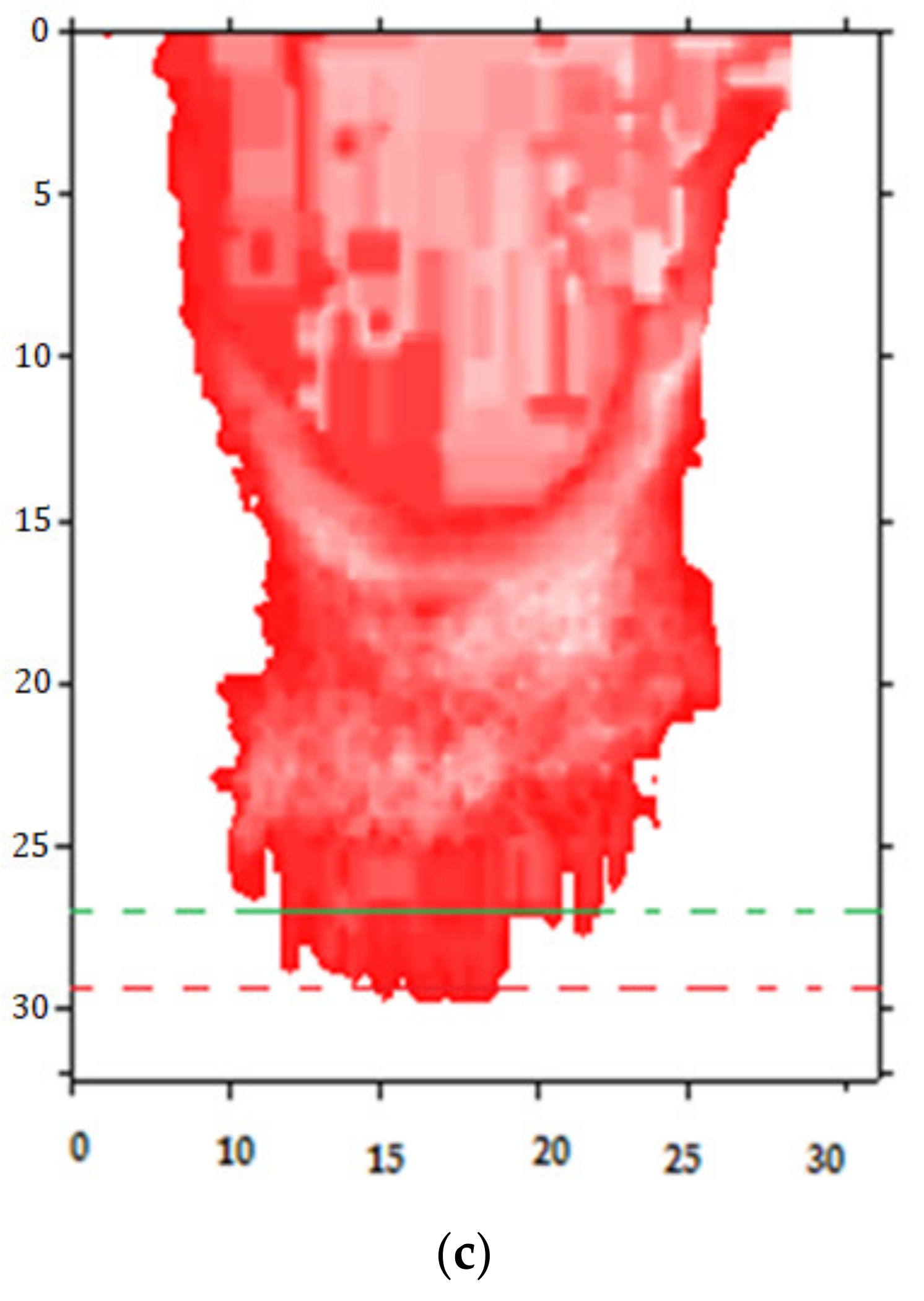
• Diesel was used as a representative of LNAPL with three different volumes, 50 mL, 100 mL, and 150 mL.
• The water table was set at 29 cm from the bottom of the column.
• The image analysis results provided quantitative time-dependent data on the LNAPL distribution through the duration for the experiments.
• Results demonstrated that the higher diesel volume (150 mL) exhibited the faster LNAPL migration through all experiments. This observation was due to the high volume of diesel as compared to other cases which provides high pressure to migrate deeper in a short time.
• In all experiments, the diesel migration was fast during the first few minutes of observation, and then the velocity was decreased gradually. This is due to pressure exerted by diesel in order to allow the diesel to percolate through the sand voids.
• Overall, this study proved that the image analysis can be a good and reliable tool to monitor the LNAPL migration in porous media.
• The results of the study confirm the viability of SIAM to be used as a laboratory tool to assess the behavior of fluids in soil and subsurface as compared to other image analysis such as light transmission visualization as well as light reflection method [2].

References

1. Agaoglu, B.; Copty, N.K.; Scheytt, T.; Hinkelmann, R. Interphase mass transfer between fluids in subsurface formations: A review. Adv. Water Resour. 2015, 79, 162–194. [Google Scholar] [CrossRef]
2. Alazaiza, M.Y.D.; Ngien, S.K.; Bob, M.M.; Ishak, W.M.F.; Kamaruddin, S.A. An overview of photographic methods in monitoring non-aqueous phase liquid migration in porous medium. Spec. Top. Rev. Porous Med. Int. J. 2015, 6, 367–381. [Google Scholar] [CrossRef]
3. Huling, S.G.; Weaver, J.W. Ground Water Issue: Dense Nonaqueous Phase Liquids; US Environmental Protection Agency: Washington, DC, USA, 1991. [Google Scholar]
4. Alazaiza, M.Y.D.; Ngien, S.K.; Bob, M.M.; Kamaruddin, S.A.; Ishak, W.M.F. Non-aqueous phase liquids distribution in three-fluid phase systems in double-porosity soil media: Experimental investigation using image analysis. Groundw. Sustain. Dev. 2018, 7, 133–142. [Google Scholar] [CrossRef]
5. Ngien, S.K.; Rahman, N.A.; Bob, M.M.; Ahmad, K.; Sa’ari, R.; Lewis, R.W. Observation of light non-aqueous phase liquid migration in aggregated soil using image analysis. Trans. Porous Med. 2012, 92, 83–100. [Google Scholar] [CrossRef]
6. Amr, S.S.A.; Alazaiza, M.Y.D.; Bashir, M.J.; Alkarkhi, A.F.; Aziz, S.Q. The performance of S2O82−/Zn2+ oxidation system in landfill leachate treatment. Phys. Chem. Earth 2020, 120, 102944. [Google Scholar] [CrossRef]
7. Alazaiza, M.Y.D.; Ngien, S.K.; Bob, M.M.; Kamaruddin, S.A.; Ishak, W.M.F. Quantification of dense nonaqueous phase liquid saturation in double-porosity soil media using a light transmission visualization technique. J. Porous Med. 2017, 20, 591–606. [Google Scholar] [CrossRef]
8. Pankow, J.F.; Cherry, J.A. Dense Chlorinated Solvents and Other DNAPLs in Groundwater: History, Behavior, and Remediation; Waterloo Press: Portland, OR, USA, 1996. [Google Scholar]
9. Sale, T.; Newell, C.J. Impacts of Source Management on Chlorinated Solvent Plumes. In Situ Remediation of Chlorinated Solvent Plumes; Springer: Berlin/Heidelberg, Germany, 2010. [Google Scholar]
10. Engelmann, C.; Händel, F.; Binder, M.; Yadav, P.K.; Dietrich, P.; Liedl, R.; Walther, M. The fate of DNAPL contaminants in non-consolidated subsurface systems–Discussion on the relevance of effective source zone geometries for plume propagation. J. Hazard. Mater. 2019, 375, 233–240. [Google Scholar] [CrossRef] [PubMed]
11. Aydin, G.A.; Agaoglu, B.; Kocasoy, G.; Copty, N.K. Effect of temperature on cosolvent flooding for the enhanced solubilization and mobilization of NAPLs in porous media. J. Hazard. Mater. 2011, 186, 636–644. [Google Scholar] [CrossRef] [PubMed]
12. Kokkinaki, A.; O’Carroll, D.; Werth, C.J.; Sleep, B. An evaluation of Sherwood–Gilland models for NAPL dissolution and their relationship to soil properties. J. Contam. Hydrol. 2013, 155, 87–98. [Google Scholar] [CrossRef]
13. Karaoglu, A.G.; Copty, N.K.; Akyol, N.H.; Kilavuz, S.A.; Babaei, M. Experiments and sensitivity coefficients analysis for multiphase flow model calibration of enhanced DNAPL dissolution. J. Contam. Hydrol. 2019, 225, 103515. [Google Scholar] [CrossRef]
14. Alazaiza, M.Y.D.; Copty, N.K.; Abunada, Z. Experimental investigation of cosolvent flushing of DNAPL in double-porosity soil using light transmission visualization. J. Hydrol. 2020, 584, 124659. [Google Scholar] [CrossRef]
15. Niemet, M.R.; Selker, J.S. A new method for quantification of liquid saturation in 2D translucent porous media systems using light transmission. Adv. Water Resour. 2001, 24, 651–666. [Google Scholar] [CrossRef]
16. Bob, M.M.; Brooks, M.C.; Mravik, S.C.; Wood, A.L. A modified light transmission visualization method for DNAPL saturation measurements in 2-D model. Adv. Water Resour. 2008, 31, 727–742. [Google Scholar] [CrossRef]
17. Belfort, B.; Weill, S.; Lehmann, F. Image analysis method for the measurement of water saturation in a two-dimensional experimental flow tank. J. Hydrol. 2017, 550, 343–354. [Google Scholar] [CrossRef] [Green Version]
18. Alazaiza, M.Y.D.; Ramli, M.H.; Copty, N.K.; Sheng, T.J.; Aburas, M.M. LNAPL saturation distribution under the influence of water table fluctuations using simplified image analysis method. Bull. Eng. Geol. Environ. 2020, 79, 1543–1554. [Google Scholar] [CrossRef]
19. Kamon, M.; Endo, K.; Katsumi, T. Measuring the k–S–p relations on DNAPLs migration. Eng. Geol. 2003, 70, 351–363. [Google Scholar] [CrossRef]
20. Tidwell, V.C.; Glass, R.J. X ray and visible light transmission for laboratory measurement of two-dimensional saturation fields in thin-slab systems. Water Resour. Res. 1994, 30, 2873–2882. [Google Scholar] [CrossRef]
21. Alazaiza, M.Y.D.; Ramli, M.H.; Copty, N.K.; Ling, M.C. Assessing the impact of water infiltration on LNAPL mobilization in sand column using simplified image analysis method. J. Contam. Hydrol. 2021, 238, 103769. [Google Scholar] [CrossRef]
22. Yilmaz, I.T.; Gumus, M.; Akçay, M. Thermal barrier coatings for diesel engines. In Proceedings of the International Scientific Conference, Gabrovo, Bulgaria, 19–20 November 2010; pp. 19–20. [Google Scholar]
23. Gallage, C.; Kodikara, J.; Uchimura, T. Laboratory measurement of hydraulic conductivity functions of two unsaturated sandy soils during drying and wetting processes. Soils Found 2013, 53, 417–430. [Google Scholar] [CrossRef] [Green Version]
24. Liu, Q.; Yasufuku, N.; Miao, J.; Ren, J. An approach for quick estimation of maximum height of capillary rise. Soils Found 2014, 54, 1241–1245. [Google Scholar] [CrossRef] [Green Version]
25. Day, R.W. Foundation Engineering Handbook. In Design and Construction with 2006 International Building Code; McGraw-Hill: Sydney, Australia, 2005. [Google Scholar]
26. Terzaghi, K.; Peck, R. Soil Mechanics in Engineering Practice; Wiley: New York, NY, USA, 1948. [Google Scholar]
27. Simantiraki, F.; Aivalioti, M.; Gidarakos, E. Implementation of an image analysis technique to determine LNAPL infiltration and distribution in unsaturated porous media. Desalination 2009, 248, 705–715. [Google Scholar] [CrossRef]
28. Alazaiza, M.Y.D.; Ngien, S.K.; Copty, N.; Bob, M.M.; Kamaruddin, S.A. Assessing the influence of infiltration on the migration of light non-aqueous phase liquid in double-porosity soil media using a light transmission visualization method. Hydro. J. 2019, 27, 581–593. [Google Scholar] [CrossRef]
Figure 1. Experimental setup.
Fluids 06 00189 g001
Figure 2. The behavior of 50 mL diesel volume in capillary fringe and water table.
Fluids 06 00189 g002
Figure 3. The behavior of 100 mL diesel volume in capillary fringe and water table.
Fluids 06 00189 g003
Figure 4. The behavior of 15 × 0 mL diesel volume in capillary fringe and water table.
Fluids 06 00189 g004
Figure 5. Samples of the image analysis showing the diesel behavior using (a) 50 mL, (b) 100 mL, and (c) 150 mL.
Fluids 06 00189 g005aFluids 06 00189 g005b