
A Study of RANS Turbulence Models in Fully Turbulent Jets: A Perspective for CFD-DEM Simulations


Norman B. Keevil Institute of Mining Engineering, Faculty of Applied Science, University of British Columbia, 517-6350 Stores Road, Vancouver, BC V6T 1Z4, Canada
*
Authors to whom correspondence should be addressed.
Fluids 2021, 6(8), 271; https://0-doi-org.brum.beds.ac.uk/10.3390/fluids6080271
Submission received: 19 June 2021
/
Revised: 23 July 2021
/
Accepted: 28 July 2021
/
Published: 31 July 2021
(This article belongs to the Collection Advances in Turbulence)
Abstract
:This paper presents an analysis of linear viscous stress Favre averaged turbulence models for computational fluid dynamics (CFD) of fully turbulent round jets with a long straight tube geometry in the near field. Although similar work has been performed in the past with very relevant solutions, considerations were not given for the issues and limitations involved with coupling between an Eulerian and Lagrangian phase, such as in fully two-way coupled CFD-DEM. These issues include limitations on solution domain, mesh cell size, wall modelling, and momentum coupling between the two phases in relation to the particles size. Therefore, within these considerations, solutions are provided to the Navier–Stokes equations with various turbulence models using a three-dimensional wedge long straight tube geometry for fully developed turbulence flow. Simulations are performed with a Reynolds number of 13,000 and 51,000 using two different tube diameters. It is found that a modified k- turbulence model achieved the most agreeable results for both the velocity and turbulent flow fields between these two flow regimes, while a modified k- SST/BSL also provided suitable results.
1. Introduction
Round turbulent jets have a wide range of applications that include combustion, jet cutting, and surface coating and they have been studied extensively, numerically and using experiments. The turbulent round jets can be categorized into three main groups: (i) particle-laden jets, (ii) impinging jets, and (iii) free round jets, each of which has distinct geometries. A long straight tube nozzle is commonly found in particle-laden jets applications with the particle mixture injected into the inlet. The choice of the particle-laden flow geometry is driven by the need to achieve fully developed flow before the nozzle exit to help quantify spreading rates with variations of particle diameters and Stokes number with a higher accuracy. This is demonstrated in the papers given by [1,2,3,4], in which 93, 90, and 163 nozzle diameters are used for the lengths of the nozzles, and the flow fully develops by the nozzle exit. Similar long nozzles are also shown in many other studies, including [5,6,7,8,9]. Using test cases that have fully developed flow provide consistency between the boundary conditions of the numerical simulations and input parameters of the experimental data.
The geometries for the application of impinging jets range from a smooth contraction to straight nozzles, and they may or may not have fully developed flow [10]. The free jets typically have contraction or sharp edged slots without fully developed flow [11].
There have been a plethora of numerical studies over the past years on jet turbulence modelling as shown in Table 1, but the geometries and operating parameters are not common across these studies. This difference is because the focus is on pure, single-phase CFD simulations without the considerations and issues indicative of CFD-DEM coupling.
The most common way to model a jet in numerical simulations is using a fixed boundary condition taken from DNS or experimental data for pipe flow. This circumvents the use of a nozzle in the solution domain and wall functions or eliminates the requirement for resolving the boundary layer. Although this is the best solution for fundamental single-phase flow problems, determining an optimum nozzle shape for particle-laden jets using CFD-DEM simulations requires that the nozzle profile shape be included in the solution domain. This is due in part to the location and initial operating parameters for particle insertion. Particles could be inserted at the nozzle exit, but this would require experimental data for each change in nozzle shape, which would be impractical for any type of industrial flow problem. Therefore, to tune these RANS turbulence models, a length of nozzle is included in the solution domain to ensure that the shear layer along the nozzle wall and the resulting boundary layer separation are being modelled correctly.
It is important to realize that with the current developments in computational resources, LES turbulence modelling is the ideal candidate for many different flow problems because of its ability to model anisotropic flow behaviors. However, for some applications, such as in fully coupled Eulerian–Lagrangian flow modelling, LES is impractical or impossible because of limitations related to mesh size for sufficient resolution of turbulent eddies and wall modelling. Therefore, for such applications, RANS turbulence models are a viable option. It should be noted that many studies have been performed using CFD-DEM and LES for jet flow, but a one-way coupled regime have been used. Although one-way coupled simulations may be adequate for dilute flows, particle–particle and particle–fluid interactions make a significant contribution to the physics of jets for dense flows [12].
RANS turbulence models are derived purely from dimensional analysis and some intuition in theory. Coefficients are then used to provide accurate results to a variety of general flow regimes. It would be ideal if these coefficients were set from principle values, such as kinetic theory of gases, but instead, they are empirically set for a variety of general flow regimes. This has been proven to be accurate in many cases but has shown inaccuracy in capturing the spreading rates for round jets [13,14].
Researchers have implemented and tested many methods to circumvent this issue, such as adding vortex stretching, cross diffusion terms, and, also, modification of the empirical coefficients, and this has provided accurate results with a constant edged boundary condition. However, very few studies have been performed for long straight tube geometries that arise in fully coupled CFD-DEM simulations and optimization problems. Therefore, this present paper’s contribution is modification and then testing of RANS turbulence models for the application of long straight tube jet flow that are required for CFD-DEM simulations to ensure that the results are agreeable to the experimental data.
2. Numerical Methodology
2.1. Background
In experiments, anisotropic turbulence behavior is observed in high-speed jet flow due to the strong boundary layer separation at the exit of the nozzle, which makes this type of flow difficult to model. This anisotropic turbulence has also been demonstrated in numerical simulations when using LES Bonelli et al. [22]. RANS turbulence models studied in this paper use the very common linear viscous Boussinesq approximation that assumes that the momentum transfer caused by turbulence can be modelled by an eddy viscosity. In using this model, we assume that the eddy viscosity is independent of direction and, hence, the rate of turbulence generation is uniform in all directions. This is not to say there is no anisotropic turbulence when using these types of models, because the mean strain rate tensor of the velocity field in the Navier–Stokes equations is not necessarily isotropic. Suffice to say, there is an expected error in using RANS approaches because of anisotropy, but if we can capture an average quantification, then we can achieve results that are sufficient for understanding of the flow behavior while achieving adequate single-phase results before the addition of particles in unresolved fully coupled CFD-DEM simulations.
Turbulent round jets have been difficult to model numerically since the beginning of RANS turbulence modelling by producing spreading rates that are not agreeable. This is shown in many papers, including Pope [13], Quinn and Militzer [11], Launder and Spalding [23], Morgans et al. [17], Givi and Ramos [15], and also stated in David C. Wilcox’s famous book Turbulence modelling for CFD [14]. RANS turbulence models have empirical coefficients that have been adjusted for generalized flow conditions. In an ideal world, these coefficients would be set from principle values, such as in kinetic theory of gases. Instead the developed RANS turbulence models are derived from dimensional analysis and some intuition on theory and, therefore, the coefficients are merely empirical providing agreeable results for a wide range of generalized flow conditions. Free shear flows, such as jet flows, are one of these generalized flow conditions.
In 1978, Pope suggested that changing the constant, , in the k- model will solve the issue with round/plane jets, but states that this goes against any kind of generality [13,17]. That being said, researchers have adopted the method of changing and it is perfectly valid because, as stated before, these coefficients are merely empirical relations to fit to a generalized flow regime [14,15,17,20]. Instead, Pope proposed a modification to the k- model by adding a vortex stretching variable to the destruction of turbulence term. The equation in the standard k- model is modified by
where, is the non-dimension measure of vortex stretching given by
and and are the mean-rotation and mean-strain rate tensors defined as
In the OpenFOAM tensor library, Equations (3) and (4) can be obtained by decomposing to the skew and symmetric parts of the gradient of velocity, U, respectively. That is: and . The theory is that the primary mechanism of turbulent energy dissipation is through stretching of the vortex rings in three-dimensions, but not in two-dimensions. Rubel [24] tested this model and determined that while this correction helps rectify the problems with round jet modelling, plane jet modelling was still experiencing problems. Because, exclusively, three-dimensional wedge simulations are considered in this work, the issues with plane jet modelling are ignored.
Contrasting from the k- model, the Wilcox k- turbulence model produces spreading rates for the round nozzle that are comparable, but larger, than predicted spreading rates for the plane jets [25]. To solve this issue for the plane jets while conserving the correct predicted values for round jets, Wilcox realized that, when the constant is reduced to 0.06 from 0.0708, the predicted spreading rates for both the round and plane jets were close to the experimental values. Rather then changing the value of the constant, Wilcox proposed a more “general” solution that reformulates the k- model by
where
Although this may solve the issue with the round/plane jet anomaly, the k- turbulence model is sensitive to free-stream boundary conditions; this could present an issue in determining a solution that is invariant with different initial free-stream conditions [25,26] and, to that affect, this turbulence model is not considered in this present work.
In this present work, we compare the velocity and kinetic energy profiles for various wall function RANS approaches to turbulence modelling. Two distinct test cases are considered with a Reynolds number of 13,000 for the test case given by Hardalupas et al. [1] and 51,000 for the test case given by Bogusławski and Popiel [27].
2.2. Numerical Model
The fluid flow in the present research is described by the Navier–Stokes equations given by
where, u is the fluid velocity, p is the pressure, is the density of the fluid, is the viscosity of the fluid, and x is a unit in space. It should be noted that the assumption of an incompressible flow is made in this work since the considered velocities are far from the sonic velocity and, therefore, the following term becomes
but is still included in the formulation for solution boundedness.
Turbulent flows can be calculated for each point in the flow field by solving the Navier–Stokes Equations (7) and (8), directly; this approach is called direct numerical simulations (DNS). For this to be accurate, all the spatial and temporal turbulent scales need to be resolved, requiring an extremely fine mesh with a number of mesh points satisfying , which is extremely computationally expensive. Less costly alternatives are to solve for the mean pressure and velocity fields using a Reynolds averaged approach (RANS), or to solve for the large scales directly while modelling the subgrid scale turbulence by the use of a large eddy simulation approach (LES).
Assuming that the velocity and pressure can be described by the mean and fluctuation components, and , and with some lengthy reductions the Navier–Stokes equations become the RANS equations given by
where, RANS Reynolds stress term. By examining the difference between the Navier–Stokes (Equations (7) and (8)) and the RANS it can be realized that the difference between them is a Reynolds stress term, and the use of mean pressure and mean velocities instead of instantaneous. This is an important realization during code development because we can merely specify an additional term when RANS or LES filtering is desired for turbulence modelling. It should be noted that many CFD codes use this method, including OpenFOAM. The Reynolds stress term, , now needs to be modelled to close the RANS equations. We can calculate the Reynolds Stress term directly with the addition of six transport equations, but this approach is expensive. There are single transport equation models, such as the mixing-length and Sparlat–Allmaras, but their accuracy is lacking. The most common method, with a good balance in required computational resources and accuracy, is the use of an eddy viscosity turbulence model with two transport equations, such as the k-, k-, and their variants.
The Boussinesq eddy viscosity assumption is now used to model the Reynolds stress tensor for both subgrid LES and RANS turbulence models. The Boussinesq eddy viscosity assumption for the Reynolds Stress with incompressibility is given by
where the first term on the right hand side is the deviatoric part, the second is the isotropic part, and k is specific kinetic energy. We then plug Equation (11) into Equation (10) to obtain the Navier–Stokes momentum equation in the OpenFOAM code.
where is the turbulent viscosity and is a modified mean pressure that has absorbed the isotropic part of the Reynolds stress term.
It is now prudent to discuss the Navier–Stokes in relation to fully coupled unresolved CFD-DEM simulations to gain a better understanding on why a wall function approach with a coarser mesh is required. Coupling between the carrier phase and solid phase involves the use of volume fraction of solids with the Navier–Stokes equations given by
where is the liquid phase volume fraction, is the liquid fluid velocity, is the mean solid particle velocity, is the liquid phase stress tensor, is the implicit momentum source term that is a volume average of all interacting forces acting on the solid phase due to the motion of the fluid in each cell, and f is any other explicit forces acting on the fluid.
As can be realized by the Equations (14) and (15), the momentum of the fluid is highly dependent on the volume fraction of solids, , and hence, the calculation of this term is critical to obtain accurate physics. The most accurate solution to this would be to calculate the volume of the particle ratios directly in the carrier phase cells, but this is impractical because it would be extremely inefficient. Instead, a volume fraction model is used that allows efficient computation while providing reasonable results for accurate flow physics. To ensure that this model is correct, the particle size to cell size ratio must have minimal particle overlap [28,29]. It is, therefore, unfeasible to fully resolve the boundary layer and have an overall fine mesh in these types of simulations unless the desired particle size is extremely small.
2.2.1. Turbulence Models
The most common two-equation eddy viscosity turbulence models can be categorized into k- and k- turbulence models with variants. Here, an equation for turbulent kinetic energy, k, and for a turbulence length scale, typically using or , are used. The k- model is the more popular of the two, with the generalized formulation given by
where eddy viscosity is given by and the Boussinesq assumption is used to obtain
and k is the turbulent kinetic energy, is the turbulent dissipation rate, u is fluid velocity, f is a damping function, and the turbulence length scale is given by . Table 2 shows the values or formulations of the generalized variables for the standard Launder and Spalding [23], variants, and modified k- turbulence models.
For the Chien model we make an estimation for the non-dimensional wall distance, . Wallin and Johansson [34] demonstrated that the non-dimensional wall distance as a function of kinetic energy is approximately equal to the non-dimensional wall distance as a function of fluid velocity for ; that is, for . With this in mind, Wallin and Johansson [34] suggested using an alternative scaling of viscosity given by
It should be noted that at . For the RNG turbulence model , , .
For completeness, we will state the previously mentioned Pope correction to the standard Launder and Spalding [23] k- turbulence model given by
where the non-dimensional measure of vortex stretching term, , is computed by first performing the inner product of the two mean-rotation rate tensors and then by calculating the double inner product of the resultant and the mean-strain rate tensor. The coefficients for the Pope correction are equal to that of the standard k- model with the additional constant providing the most agreeable results for the respective geometry and boundary condition tested in the original paper. The coefficients provided for these models are empirical relations that have been fit for generalized flow problems. Realizing this, along with the issues with the jet flow modelling, Tam and Ganesan [35] performed many jet flow experiments to determine a new set of coefficients that will allow accurate modelling of the jet flow for a variety of Reynolds numbers and geometries. This set of coefficients are given by , , , , , . It is noted that the diffusion coefficients and are significantly smaller than the standard coefficients and can be characterized by an increase in diffusion of k and because of their location in the denominators of Equations (16) and (17). These coefficients will be used in the present work with the naming as Tam-Thies KE. Slight modifications to the empirical constants in the Launder and Spalding [23] are also used with “mod1” having the change of similarly performed by Quinn and Militzer [11] and Faghani et al. [20] and “mod2” having the change of and similarly performed by Givi and Ramos [15].
2.2.2. k- Turbulence Models
The standard k- model is given by a production term of turbulent kinetic energy, k, and frequency of dissipation, . Kolmogorov, in 1941, was the first to suggest the two-equation turbulence model for kinetic energy and dissipation per unit turbulence kinetic energy [36]. Unaware of Kolmorgorov’s work, Saffman [37] produced a k- model that had better agreement than Kolmorgorov’s, and has served as the basis of “modern” k- turbulence models. One of the most influential contributors to the k- turbulence model was the work performed by David C. Wilcox. A sequential timeline of Wilcox’s work will not be stated, and since no modifications to this model have been performed in the present work, the reader is encouraged to review the paper given in Wilcox [25] for details on the model.
The goal of the k- SST and BSL turbulence models is to use the k- model due to its robustness near the wall, and then transition to the k- model for its effectiveness in the far field. This is achieved using a blending function, , that is a function of wall distance with k- and “transformed“ k- models. When the value of is equal to one, then the k- proposed by Wilcox [38] is used. When is equal to zero, then a transformed version of the standard k- model of Launder and Spalding [23] is used. It should be noted here that the “transformed” k- model is typically stated to be an exact transformation of the k- model, but this is erroneous to state because terms are dropped in the derivation. This will be discussed further in this paper.
To better understand this model and determine its ability to adapt to turbulent jet flow conditions, the BSL/SST turbulence models [39] with the updated modifications [40] will first be stated, followed by an in depth study on the origins of the model to determine if the coefficients are likely candidates for modification. The BSL model is given by
where, , , , and are constants, , that are calculated using the equation . The k- model, , constants are taken directly from Wilcox [38] to be , , and by ensuring that . The constants for the “transformed” k- model, , are given by , , =0.0828, and with . These are used to mimic the constants given by the standard k- model of Launder and Spalding [23].
As previously stated, the k- BSL/SST turbulence model uses the standard 1988 Wilcox k- turbulence model in the near field and transitions to a “transformed” k- in the far field. The “transformed” k- equation is derived by a change in dependent variables from to using the relation defined by with the standard k- Launder and Spalding [23] model. Specifically, for kinetic energy the model becomes
and for rate of dissipation
If we then compare this fully derived transformed k- formulation with the model given from Menter [26], it is observed that the equation for turbulent kinetic energy is equivalent, but that some terms are dropped in the rate of dissipation equation. Specifically, fluid viscosity in the cross diffusion term given by
and terms for turbulent diffusion given by
In his book “Turbulence Modelling for CFD”, Wilcox [14] states that “focusing on free shear flow, we can ignore molecular viscosity”. Perhaps the contribution of molecular viscosity has an insignificant contribution with the application to free sheer flows, but this does not explain why the model can be applied to applications other than free shear flows. Wilcox also states that if we assume for simplicity, then the terms for turbulent diffusion given by Equation (28) can be dropped. It can, therefore, be argued that this is not an “exact” transformation of the standard k- model. That being said, this is not a problem, since the k- is not any more fundamental than the k- model; with the only difference in transformation method. Therefore, the modifications that have been performed for the standard k- model in jet flow, both in this work and by other researchers, do not necessarily carry over to the “transformed” k- model.
We can dive into this analysis further by relating the empirical coefficients between the standard and “transformed” k- turbulence models. It is realized that the coefficients chosen for the “transformed” k- model directly mimic that of the standard k- model for and , where for the “transformed” and for the derived version. It is still unclear whether this adjustment makes a significant contribution to a solution, but it should be noted nevertheless.
All this being said, if the standard k- model produces spreading rates that are not agreeable, then it makes sense that the k- BSL model will produce spreading rates similar to the standard k- and, therefore, some modification of the empirical coefficients need to be performed to provide “more” agreeable results. To directly mimic the modification of the the k- model, we set and relate the constants from the k- to the transformed k- model by . This will be aptly named for the k- SST/BSL models in the solution results. It should be noted that although other researchers have modified the empirical constants for the k- in the past [11,15,17,20], to the present authors’ knowledge there has been no one that has modified the constants in k- SST/BSL models other than the developer of the turbulence model themselves. Therefore, results for the modified k- SST/BSL models should not be indicative as a general solution for a variety of jet flows unless further testing is performed.
The SST model is the most commonly used model proposed by Menter [39] that is differentiated from the BSL model through a change in coefficients, turbulence viscosity, and blending functions. The coefficients for the SST turbulence model are given by
and turbulent viscosity is given by
where, is the vorticity magnitude calculated as , and y is the distance from the centre of the cell to the wall. It should be noted that because of the change in eddy viscosity relative to the BSL model (), the production term in the dissipation equation for k- SST model is equal to instead of .
There have since been updates to the original [39] model given in Menter et al. [40] that provide more agreeable solutions in industrial flow applications and is considered the “standard” model, so we will name this model SST std. to avoid confusion. The most significant change is that of eddy viscosity, from the use of the magnitude of vorticity to the magnitude of the strain invariant.
where, . A turbulent production limiter is also used to avoid turbulence production in the stagnation regions for both k and , as given by
is changed by the use of instead of ,
and some constants are changed, specifically, and . The default k- SST that is implemented in OpenFOAM is a modification of the original SST model. The origins of these modifications are unclear because of lack of a reference, but it is very similar to the original SST model and will be labelled SST def. in all the results.
3. Simulation Setup
Two distinct cases are considered that are separated by geometry and flow conditions. Namely, cases that follow the work performed by Hardalupas et al. [1] and Bogusławski and Popiel [27]. The operating parameters chosen for the simulations are taken directly from the inputs in the respective papers and if an assumption was needed then an explanation and justification will be shown.
3.1. Hardalupas et al. Test Case
Hardalupas et al. [1] use a phase-Doppler anemometer to measure the velocity and flux distributions in both clean jet (with seeding powders) and particle-laden high-speed air jets. The flow is fully developed in a 15 mm diameter nozzle of 93 nozzle diameters in length. An average velocity of 13 m/s is used that correlates to a Reynolds number of 13,000.
3.2. Bogusławki and Popiel Test Case
The experiments performed in the study of Bogusławski and Popiel [27] use an air jet issued from a long straight tube of 38.5 mm in diameter and in length. The velocity and turbulence characteristics are measured using a constant temperature thermo-anemometer. This paper defines 20 m/s that corresponds to a Reynolds number, 51,000, but then uses this same as the maximum centreline velocity at the nozzle exit. This is somewhat of an ambiguity because the mean free-stream velocity in a nozzle will not be the maximum centreline velocity and, therefore, to avoid confusion the free-stream velocity, in this case will be considered the maximum centreline velocity, 20 m/s. The fixed value inlet boundary condition for the numerical simulation similarly follow the Hardalupas et al. [1] test case in that the velocity profile varies radially to the power law for turbulent jet flow with an exponent, . The boundary conditions were set to that of Table 3, where with 50,000.
3.3. Model Setup
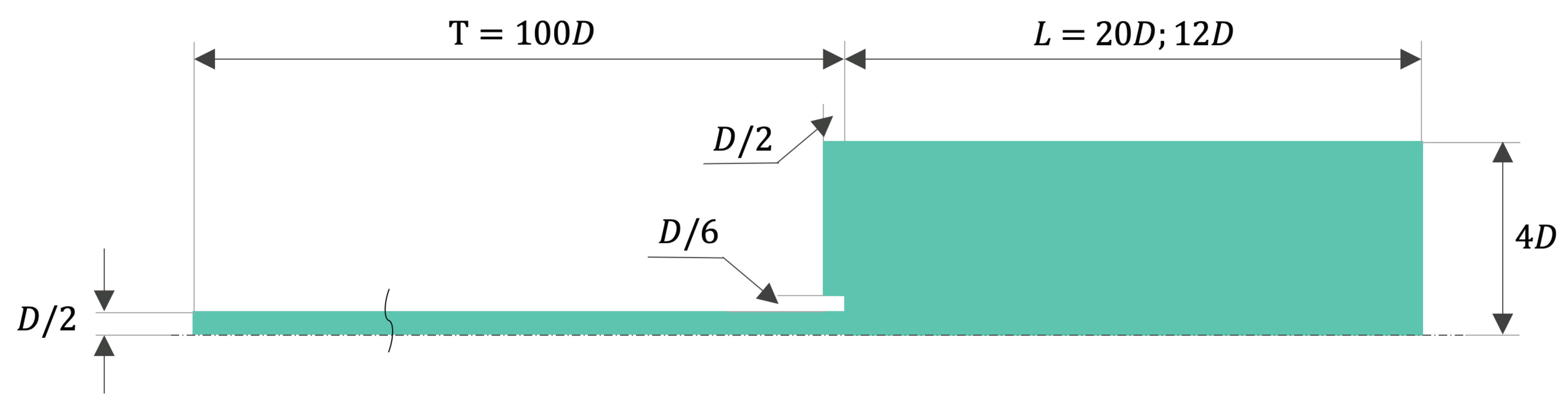
Two domains are created by taking a 5 degree wedge slice of a circular 3D domain. Figure 1 shows the geometry for both the Hardalupas et al. [1] and Bogusławski and Popiel [27] test cases. A nozzle length of 100D is used with a free-stream domain half width of 4D. A nozzle wall thickness is include in the domain with thickness D/6 and extended out towards the nozzle inlet by D/2. This is to potentially model any affects caused by boundary layer attachment at the nozzle wall. Discretization is performed using hexahedral cells generated in Ansys® ICEM CFD. Uniformly space cells of size , , and are used with a single cell being used for the width in the wedge direction.
The implicit second order backward scheme is used for temporal discretization. OpenFOAM second order linearUpwind scheme is used for all velocity and turbulent fields. This scheme uses upwind interpolation weights depending on the gradient of the fluid velocity [41]. The widely used pressure-based PISO (pressure-implicit split-operator) algorithm proposed by Issa [42] is used for the fluid solver. The OpenFOAM PCG solver with a GAMG pre-conditioner is used for pressure and PBiCG with DILU pre-conditioner used for all other fields [41]. Final solver tolerance is set to for all scalar and vector fields.
Table 3 shows the boundary conditions for the Hardalupas et al. [1] test case. The eddy viscosity near the wall is calculated from a velocity based continuous wall function that follows the Spalding’s equation [43]. The inlet velocity is set to the power law for fully developed turbulent pipe flow with the exponent, n, set equal to and a maximum velocity of . A “calculated” entry is used to signify that the turbulent viscosity is calculated from k, , and in the turbulence model. In Table 3, the turbulence intensity is equal to with . Entrainment boundary conditions are used for pressure and velocity at the domain outlet. Pressure is set to zero for outflow and set to for inflow. Velocity is set to zero gradient at all times except the tangential component is set to zero. This is used to ensure that the inflow velocity can “find” the normal component, facilitating a proper entrainment boundary.
There are many ways to calculate an initial , such as , but the most certain way is to a run a k- simulation and use the free-stream results to calculate the initial free-stream for the k- with . It was determined that an average value of 1597 will suffice for the initial free-stream values. It should be noted that this value is difficult to discern because of the boundary layer separation at the exit of the nozzle that may cause the k- Wilcox turbulence model to be inaccurate from sensitivity to free-stream input conditions [26]. The initial free-stream values were set to for kinetic energy, k, that corresponds to a turbulent intensity of .
3.4. Wall Modelling Concerns and Mesh Resolution
It is the present authors’ position that this work will serve as a basic for future work in multiphase particle-laden flows. Therefore, the meshing thought process utilized in this research has the consideration of limitations in mesh size relative to a particle diameter and the primary focus of this paper is the use of wall function approaches. In eddy viscosity RANS turbulence models, it is required to either fully integrate to the wall, or use wall function to estimate the near wall properties where viscous affects cannot be ignored. Fully integrating to the wall requires the first cell height to produce a of about 1 or less, and the first 8–10 cells located below a of about 11.5. This can cause issues with the addition of particles because of the momentum coupling between the two phases. Therefore, a good option is to use a wall function approach that will allow a larger cell near the wall with effective momentum transfer between the two phases.
The first wall functions were constructed using the Launder and Spalding methods in which it is required that the first cell height produce a in the logarithmic layer () [23]. Newer adaptive wall functions have since been proposed, which allow a wide range of values that include the more illusive buffer region. OpenFOAM uses adaptive wall function approaches proposed by Kalitzin et al. [44]. These wall functions were tested in the same work and it was realized that solutions were agreeable through a spread of values from 11 to 111, with the highest error found at . This is the wall function used in the present work.
A zero gradient boundary condition is used for kinetic energy at the wall, with wall functions for both and . In OpenFOAM, the epsilon wall function provides a constraint at the wall for both turbulent kinetic energy, k, and dissipation, [45]. The Omega wall function uses a blending of the viscous and logarithmic layer with a blending function and, theoretically, can be accurate in the buffer region. That being said, much is still unknown about the buffer region that is between the viscous and log-layer and, therefore, it is the best practice to stay out of this region as much as possible. A continuous wall function for turbulent viscosity is used, which is modelled from Spalding’s equation that fits a curve of the relationship between and [43] for the full range of the boundary layer. It should be noted that this is a function that is based on velocity or shear stress at the wall and not kinetic energy.
4. Results and Discussion
4.1. Grid Independence
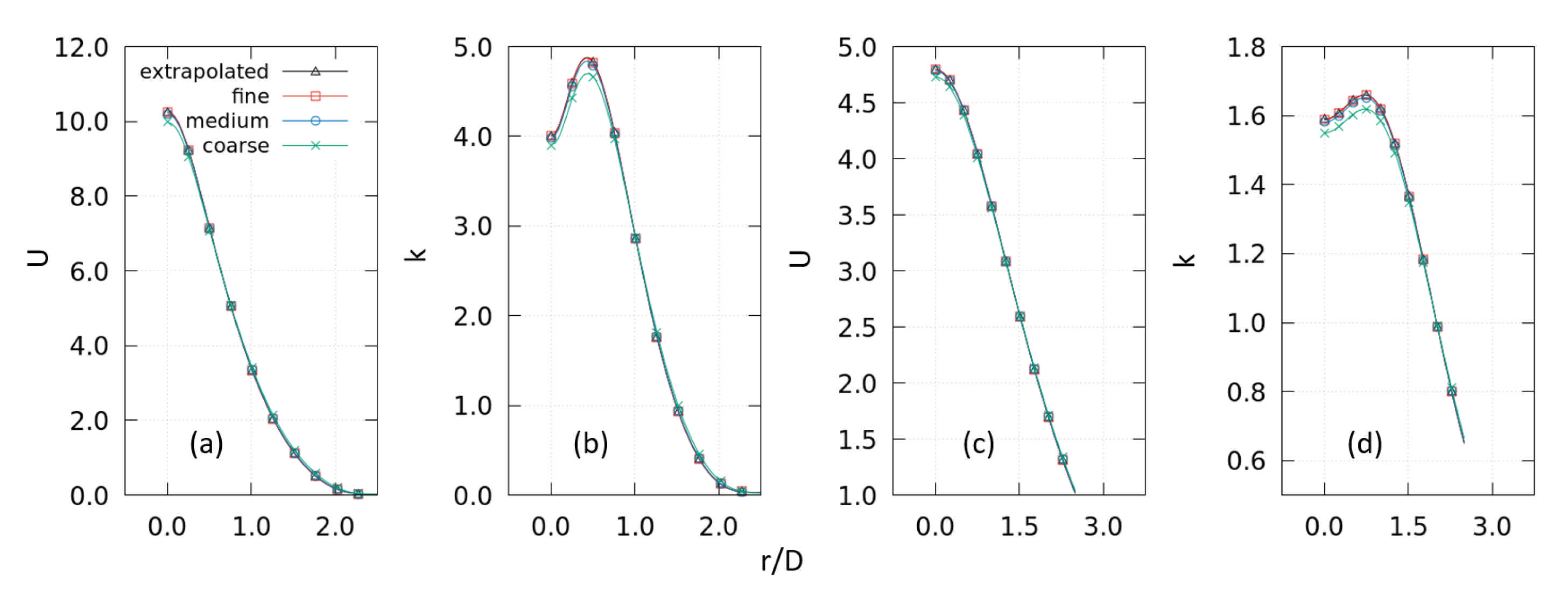
A grid sensitivity analysis is performed using the Hardalupas et al. [1] test case to determine if there are errors associated with the discretization of the fluid domain into a mesh and that the solution is independent of the mesh cell size. Three systematically refined uniformly sized meshes of 26, 85, and 100 thousand hexahedral cells are generated in ICEM© CFD meshing software with a resulting based on velocity of 27, 15, and 13, respectively.
The default k- turbulence model available in OpenFOAM is used for the grid independence with the simulation setup as described in Section 3 of this paper. It should be noted that the default k- turbulence model is the model proposed by Launder and Spalding [23]. Richardson extrapolation, as recommended by the Journal of Fluids Engineering described in Celik [46], was used to determine an extrapolated solution along a sampling line for both fluid velocity and turbulent kinetic energy (Figure 2). The fine-grid convergence index, , is then calculated for each point and averaged along the sampling line. The for velocity has a value of 0.2% for the average and 0.8% for the maximum at 10D and 0.03% for the average and 0.2% for the maximum at 20D. The for kinetic energy has a value of 0.4% for the average and 4.4% for the maximum at 10D and 0.05% for the average and 0.1% for the maximum at 20D.
The mesh of was chosen for all proceeding simulations because it was the finest mesh available that allows a reasonable value for accurate wall function modelling.
4.2. Fluid Velocity
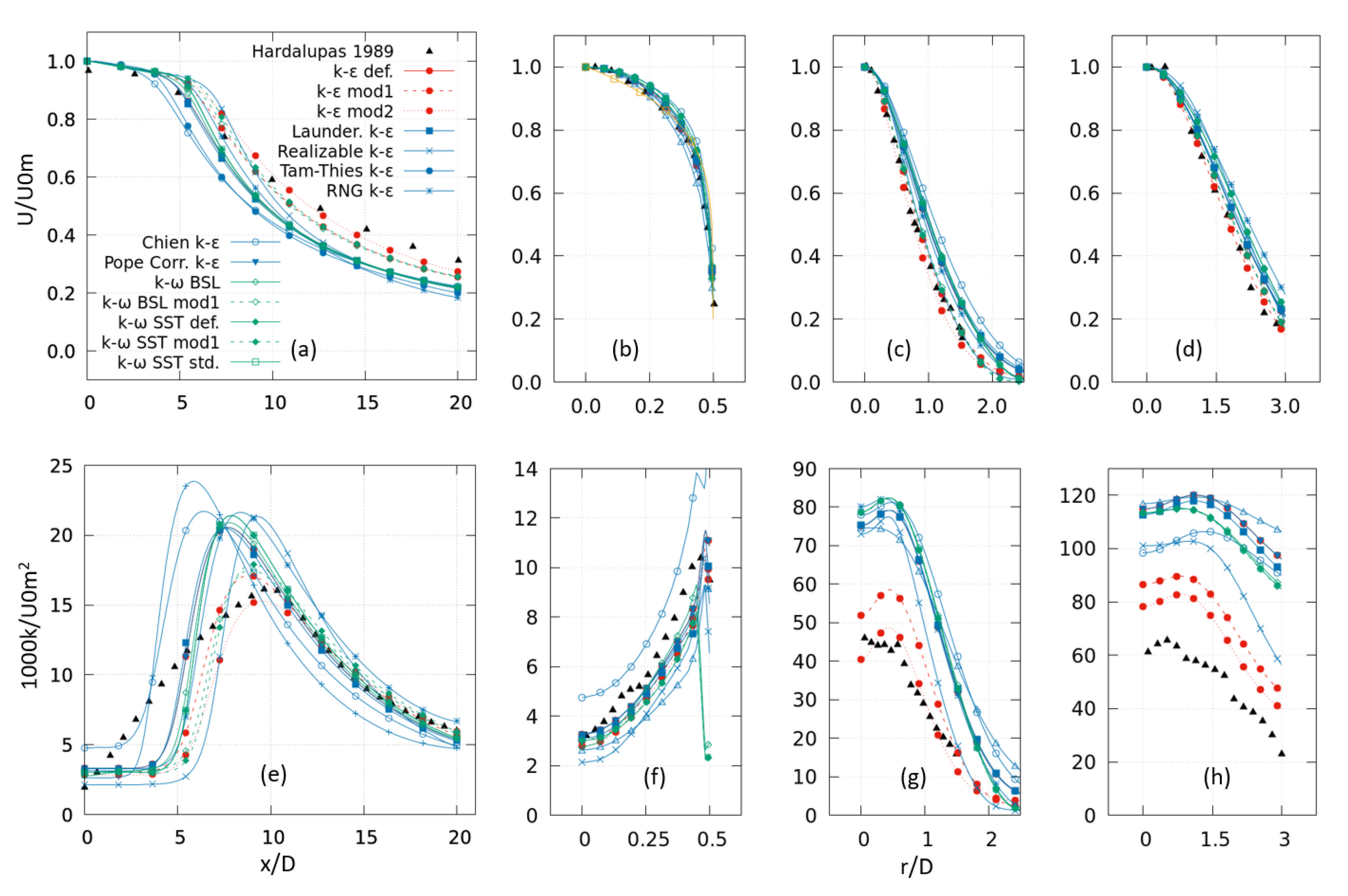
The potential core of the jet is the region in which there is a small difference in the velocity of the bulk and jet regions. The core is characterized by a conical shape narrowing from the nozzle exit to the end of the developing region. After the potential core region, the flow develops into what is known as the fully established flow field [47]. Figure 3a illustrates the velocity as a function of axial non-dimensional distance from the nozzle exit for the Hardalupas et al. [1] test case. Although it is difficult to discern exactly where the potential core ends for the experimental data because of the limited number of sampling points in the axial direction, if an extrapolation line is fitted to follow the available points, we can comment that the potential core has a length that is the most similar to the standard k-, Pope Corr. k-, and k- BSL turbulence model. The k- mod1 model with and is the most similar throughout the entire range of velocities, but has a slightly longer potential core, as shown by Givi and Ramos [15]. The conclusion, therefore, is that if merely the modelling of the potential core is desired and not the fully established flow field, then a variety of turbulence models can be used with sufficient accuracy. Nonetheless, if the full range of the near field, from the potential core through to the fully established flow (), is modelled, then the k- mod1 turbulence model is the most desired with the k- SST mod1 and k- BSL mod1 coming in a close second. This is shown for the axial and radial velocity profiles by observing Figure 3.
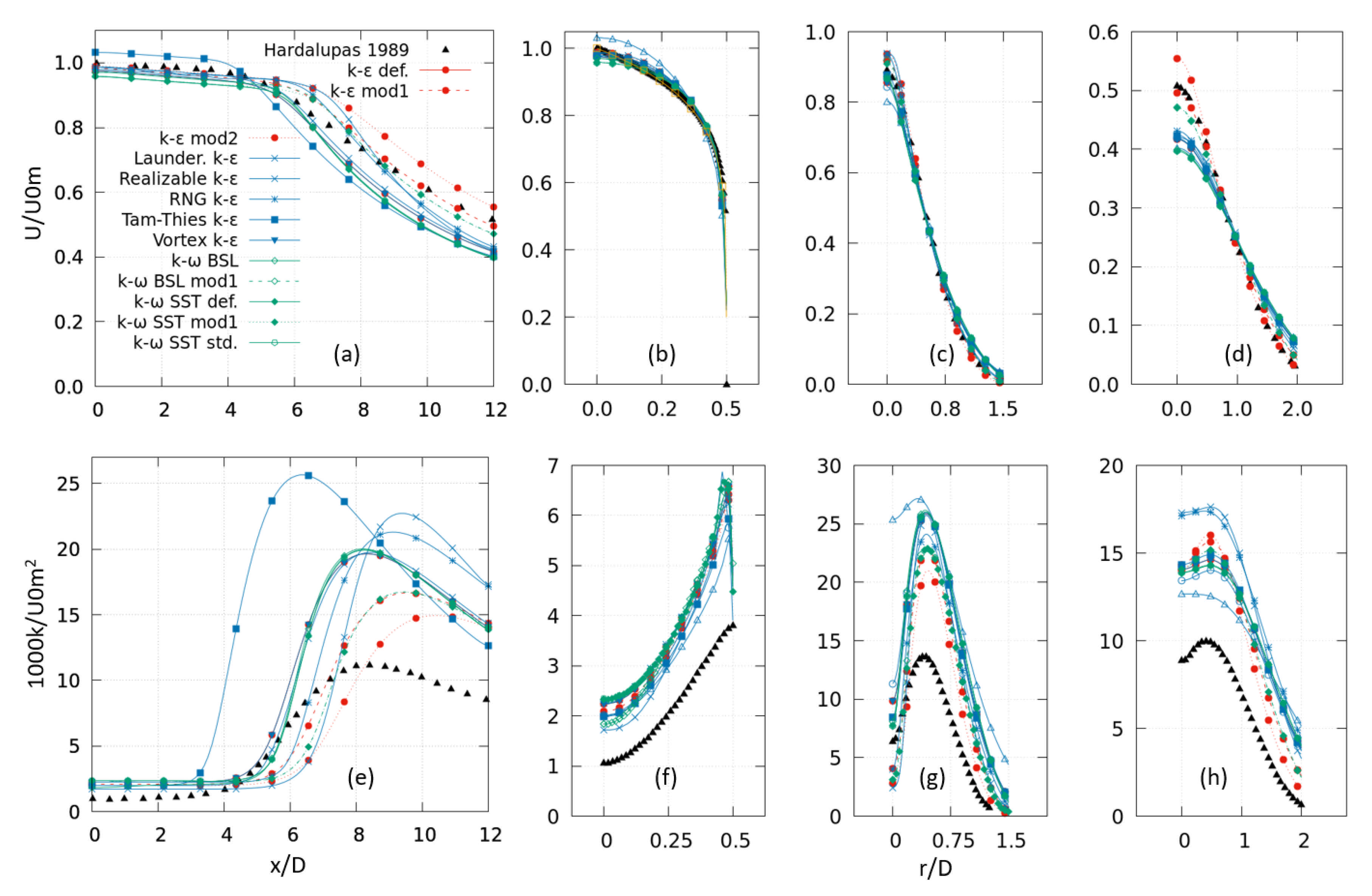
The 1/7th power law has been shown to be an accurate and simple model for profiles of fully developed turbulence pipe flow for a variety of Reynolds numbers and is plotted in orange for Figure 3b and Figure 4b. It was observed that the flow profiles for the Hardalupas et al. [1] test cases follow the 1/7th power law well for the inner region of the flow at the nozzle exit. However, the profile has a slight “U” shape, which is characteristic of a more laminar flow without a boundary layer. By observing Figure 3b it is realized that the numerical results agree more with the Hardalupas et al. [1] test case then the power law. The Bogusławski and Popiel [27] test case exhibits different behavior in that the velocity at the nozzle exit follows the 1/7th power law for both the experimental and numerical results.
It was originally thought that k- SST turbulence model, with its variants, would be the best option for these types of flow because of its ability to model the near field effectively using k- and the outer field using k-. This was found to be untrue because of the issues with empirical coefficients associated with these models. In the derivation of the k- SST/BSL turbulence models some terms are dropped and seem to be absorbed into the cross diffusion empirical coefficient of the transformed k- given by that are provided in the k- BSL/SST turbulence models.
It was found that the default k- SST model compared very well to the standard k- model in the far field. It is stated by Menter [26] that the blending function goes to zero at the log region. We observed that the value for the mesh and Reynolds numbers was about 13 for the Hardalupas et al. [1] test case and 30 for the Bogusławski and Popiel [27] test case. With this , the wall functions are fully modelling the flow field up to, or very close to, the log region for the Bogusławski and Popiel [27] test case and into the buffer region for the Hardalupas et al. [1]. Hence, for the Hardalupas et al. [1], the flow field is calculated slightly with the k- turbulence model and the rest with the “transformed” k-, while the flow field is calculated almost exclusively from the “transformed” k- for the Bogusławski and Popiel [27] test case.
Hence, the flow field is calculated from the transformed k- turbulence model for the k- SST turbulence model. The derivation of the k- SST model shows that two terms are dropped, and this does affect the results slightly with the difference between the modified and k- equation. It is thought that the constants can be further modified to account for this slight change. No previous research has investigated and reported if modifying the constants of the k- SST model would gain any benefit in the predicted flow field, and an extensive study would be required to fully understand the behavior with this type of modification and this particular aspect was not researched in this study. That being said, sufficiently accurate results using the modified k- turbulence model were achieved, which can be used for future work in round turbulence dense CFD-DEM turbulence jet flows.
It should be noted that the stated inlet velocity for the experiments performed by Bogusławski and Popiel [27] is m/s with the profile at the nozzle exit following the 1/7th power law given by
Typically the 1/7th power law velocity is normalized with the maximum centreline velocity at the nozzle exit, , and not the infinite, or mean, free-stream velocity, , and, therefore, the maximum velocity is slightly greater in magnitude than the normalized velocity. The data given from the experiments demonstrate that the definition of is not the free-stream velocity but, actually, the maximum centreline velocity at the nozzle exit, that is , because the plots never go above unity. Therefore, going forward, we will normalize the numerical data with the maximum centreline velocity, . This data treatment allows consistent normalization across each of the turbulence models because the maximum centreline velocity changes slightly between turbulence models with a constant free-stream velocity value at the inlet.
4.3. Turbulence Properties
As outlined before, when Favre averaging the Navier–Stokes equations, an additional Reynolds stress term is added that accounts for the fluctuations in the flow field. The Reynolds stress is given as a tensor by
This is a symmetric tensor and so we have gained six additional scalar transport equations in addition to the Navier–Stokes. Instead of modelling each of these six transport equations, we choose a more heuristic approach by modelling the Reynolds stress directly with the Boussinesq approximation with a linear function of the mean-strain-rate tensor using an eddy viscosity that was previously stated by Equation (11) but will also be stated here for completeness
where k is the turbulent kinetic energy defined by the one-half of trace of the Reynolds stress tensor
Therefore, the kinetic energy can be expressed by one-half of the sum of the variances, or one-half the mean square magnitude of the velocity fluctuations given as
It should be noted that the eddy viscosity is isotropic but not necessarily homogeneous and, therefore, the turbulence itself is not necessarily isotropic because the mean-strain-rate tensor of the Navier–Stokes equations is not isotropic. This is an important distinction because eddy viscosity is merely independent of direction.
To calculate turbulence kinetic energy for the experiments we use the provided root-mean-square (RMS) components of velocity given in the Hardalupas et al. [1] paper’s notation as , which is the square root of the variance equivalent to the present author’s paper notation as and . Only the radial and axial velocity components are given and, therefore, kinetic energy is in “cylindrical” coordinates and transformation can be challenging. One estimation is the so-called two-dimension approximation that is proposed by Rodriguez et al. [48]
where, to obtain Equation (39), we have a third component of turbulent kinetic energy distribution given by . This is assuming that the turbulent kinetic energy values are the same magnitude in the direction, which is not necessarily the case. It is observed by Figure 3e–h that this approximation provides results that are agreeable for the k- mod1 turbulence model but it would be unwise to make a definite conclusion with the two-dimensional assumption and, therefore, no definite conclusion for kinetic energy can be realized purely from this test case.
The turbulent kinetic energy for both cases drastically changes from a “U” shape to a “W” shape between −0.1D to 0.1D as the flow leaves the nozzle exit. It is interesting to note that a “W” shape is achieved at the nozzle exit within the range of a single nozzle diameter, 1D, in the numerical results. However, the experimental results demonstrate a “W” shape, but outside the range of 1D. This is a very important observation because it appears that the location of the hump in the W shape is not significantly different between the numerical and experimental results further in the flow field.
From Figure 4e–h it is observed that the turbulent kinetic energy in the experimental results of Bogusławski and Popiel [27] follows the overall trend well but the magnitude is significantly lower than the numerical results for all of the turbulence models tested. This was also observed in the work performed in Faghani et al. [20] and Quinn and Militzer [11]. Contrasting to this, the use of the two-dimensional approximation causes a higher magnitude in results for the Hardalupas et al. [1] test case. It is thought that this approximation is more for swirling flows causing more turbulent kinetic energy generation in the direction. The turbulence intensity in the axial direction lined up well with the experimental data, but the intensity in the other directions was about half of those achieved with the numerical results. This can be expected because of the isotropic assumption of the linear viscous RANS turbulence models ensures that the turbulence modulation is equal in all directions. Therefore, it is up to the researcher to determine if the benefits of using this type of model outweigh the potential errors. This notion is true for the use of any linear viscous RANS turbulence model because our goal is to capture the average rather then the instantaneous flow behavior.
5. Conclusions
Obtaining accurate single-phase spreading rates for jets is critical before the inclusion of particles in a CFD-DEM simulations because, otherwise, it would be difficult to attribute an agreeable answer with confidence in the CFD-DEM simulation to the correct use of models and not a combination of models that merely work for one case but not necessarily another. With this in mind, single-phase simulations have been performed in this current work to obtain agreeable single-phase results within limitations of CFD-DEM before the inclusion of particles. It is the authors intention to use this work as a base and perspective for future work in fully coupled dense two-phase CFD-DEM jet flow simulations by addressing the limitations on geometry, mesh cell size, wall modelling, and momentum coupling that occur. It was realized that a slight modification of the empirical constant = 1.5 in the standard Launder and Spalding [23] k- model provided the most agreeable results for both test cases for fluid velocity. A change in coefficients of the k- SST v1/BSL turbulence models that mimic the = 1.5 turbulence model by setting = 0.5 provided suitable results as well. It is unclear whether RANS models in general will accurately model the turbulent kinetic energy in all directions for jet flow but, as a general conclusion, the kinetic energy from the numerical results will be higher in magnitude then the experiments because this is observed for the Bogusławski and Popiel [27] test case and the work performed previously by Faghani et al. [20] and Quinn and Militzer [11]. It is, therefore, up to the researcher to weigh the costs and benefits of using these models with considerations to help quantify the errors in kinetic energy along with whether merely the velocity field is desired.
Author Contributions
Conceptualization, D.S.W. and S.M.; methodology, D.S.W.; software, D.S.W.; validation, D.S.W.; formal analysis, D.S.W.; investigation, D.S.W.; resources, S.M.; data curation, D.S.W.; writing—original draft preparation, D.S.W.; writing—review and editing S.M. and D.S.W.; visualization, D.S.W. and S.M.; supervision, S.M.; project administration, S.M.; funding acquisition, S.M. All authors have read and agreed to the published version of the manuscript.
Funding
The research is supported and funded by the MITACS Accelerate program and Disa Technologies (contract No. IT23227). We gratefully acknowledge the computing support of Compute Canada via their WestGrid program and ARC group at the University of British Columbia for providing the access to the Sockeye cluster.
Data Availability Statement
The cases, models, and data solutions are available at https://0-doi-org.brum.beds.ac.uk/10.6084/m9.figshare.15039798.v1, accessed on 19 June 2021.
Conflicts of Interest
The funders had no role in the design of the study; in the collection, analyses, or interpretation of data; in the writing of the manuscript, or in the decision to publish the results.
References
- Hardalupas, Y.; Taylor, A.; Whitelaw, J. Velocity and particle-flux characteristics of turbulent particle-laden jets. Proc. R. Soc. Lond. A Math. Phys. Sci. 1989, 426, 31–78. [Google Scholar] [CrossRef]
- Lau, T.C.; Nathan, G.J. Influence of Stokes number on the velocity and concentration distributions in particle-laden jets. J. Fluid Mech. 2014, 757, 432–457. [Google Scholar] [CrossRef] [Green Version]
- Modarress, D.; Wuerer, J.; Elghobashi, S. An Experimental Study of a Turbulence Round Two-Phase Jet. Chem. Eng. Commun. 1984, 28, 341–354. [Google Scholar] [CrossRef]
- Lau, T.C.W.; Nathan, G.J. The effect of Stokes number on particle velocity and concentration distributions in a well-characterised, turbulent, co-flowing two-phase jet. J. Fluid Mech. 2016, 809, 72–110. [Google Scholar] [CrossRef] [Green Version]
- Fan, J.; Zhang, X.; Cen, K. Laser Diffraction Method Measurements of Particle-Gas Dispersion Effects in a Coaxial Jet. Aerosol Sci. Technol. 1997, 26, 447–458. [Google Scholar] [CrossRef] [Green Version]
- Prevost, F.; Boree, J.; Nuglisch, H.J.; Charnay, G. Measurements of fluid/particle correlated motion in the far field of an axisymmetric jet. Int. J. Multiph. Flow 1996, 22, 685–701. [Google Scholar] [CrossRef]
- Sheen, H.; Jou, B.; Lee, Y. Effect of particle size on a two-phase turbulent jet. Exp. Therm. Fluid Sci. 1994, 8, 315–327. [Google Scholar] [CrossRef]
- Shuen, J.S. A Theoretical and Experimental Investigation of Dilute Particle-Laden Turbulent Gas Jets (Two-Phase Flow). Ph.D. Thesis, The Pennsylvania State University, State College, PA, USA, 1984. [Google Scholar]
- Tsuji, Y.; Morikawa, Y.; Tanaka, T.; Karimine, K.; Nishida, S. Measurement of an axisymmetric jet laden with coarse particles. Int. J. Multiph. Flow 1988, 14, 565–574. [Google Scholar] [CrossRef]
- Ashforth-Frost, S.; Jambunathan, K.; Whitney, C. Velocity and turbulence characteristics of a semiconfined orthogonally impinging slot jet. Exp. Therm. Fluid Sci. 1997, 14, 60–67. [Google Scholar] [CrossRef]
- Quinn, W.; Militzer, J. Effects of nonparallel exit flow on round turbulent free jets. Int. J. Heat Fluid Flow 1989, 10, 139–145. [Google Scholar] [CrossRef]
- Faeth, G. Mixing, transport and combustion in sprays. Prog. Energy Combust. Sci. 1987, 13, 293–345. [Google Scholar] [CrossRef] [Green Version]
- Pope, S.B. An explanation of the turbulent round-jet/plane-jet anomaly. AIAA J. 1978, 16, 279–281. [Google Scholar] [CrossRef]
- Wilcox, D.C. Turbulence Modeling for CFD, 3rd ed.; Number Book, Whole; DCW Industries: La Cãnada, CA, USA, 2006. [Google Scholar]
- Givi, P.; Ramos, J. On the calculation of heat and momentum transport in a round jet. Int. Commun. Heat Mass Transf. 1984, 11, 173–182. [Google Scholar] [CrossRef]
- Kim, K.Y.; Chung, M.K. Calculation of a strongly swirling turbulent round jet with recirculation by an algebraic stress model. Int. J. Heat Fluid Flow 1988, 9, 62–68. [Google Scholar] [CrossRef]
- Morgans, R.C.; Dally, B.B.; Nathan, G.J.; Lanspeary, P.V.; Fletcher, D.F. Applications of the Revised Wilcox 1998 K-Omega Turbulence Model to a Jet in Co-Flow. In Proceedings of the 2nd International Conference on CFD in the Minerals and Process Industries, Melbourne, Australia, 6–8 December 1999; pp. 479–484. [Google Scholar]
- Post, S.; Iyer, V.; Abraham, J. A Study of Near-Field Entrainment in Gas Jets and Sprays Under Diesel Conditions. J. Fluids Eng. 2000, 122, 385–395. [Google Scholar] [CrossRef]
- Georgiadis, N.J.; Yoder, D.A.; Engblom, W.A. Evaluation of Modified Two-Equation Turbulence Models for Jet Flow Predictions. AIAA J. 2006, 44, 3107–3114. [Google Scholar] [CrossRef] [Green Version]
- Faghani, E.; Saemi, S.D.; Maddahian, R.; Farhanieh, B. On the effect of inflow conditions in simulation of a turbulent round jet. Arch. Appl. Mech. 2011, 81, 1439–1453. [Google Scholar] [CrossRef]
- Wang, C.; Barghi, S.; Zhu, J. Hydrodynamics and reactor performance evaluation of a high flux gas-solids circulating fluidized bed downer: Experimental study. AIChE J. 2014, 60, 3412–3423. [Google Scholar] [CrossRef]
- Bonelli, F.; Viggiano, A.; Magi, V. High-speed turbulent gas jets: An LES investigation of Mach and Reynolds number effects on the velocity decay and spreading rate. Flow Turbul. Combust. 2021. [Google Scholar] [CrossRef]
- Launder, B.E.; Spalding, D.B. The numerical computation of turbulent flows. Comput. Methods Appl. Mech. Eng. 1974, 3, 269–289. [Google Scholar] [CrossRef]
- Rubel, A. On the vortex stretching modification of the k-epsilon turbulence model—Radial jets. AIAA J. 1985, 23, 1129–1130. [Google Scholar] [CrossRef]
- Wilcox, D.C. Formulation of the k-w Turbulence Model Revisited. AIAA J. 2008, 46, 2823–2838. [Google Scholar] [CrossRef] [Green Version]
- Menter, F.R. Influence of freestream values on k-omega turbulence model predictions. AIAA J. 1992, 30, 1657–1659. [Google Scholar] [CrossRef]
- Bogusławski, L.; Popiel, C.O. Flow structure of the free round turbulent jet in the initial region. J. Fluid Mech. 1979, 90, 531–539. [Google Scholar] [CrossRef]
- Weaver, D.; Miskovic, S. Analysis of Coupled CFD-DEM Simulations in Dense Particle-Laden Turbulent Jet Flow. In Proceedings of the ASME 2020 Fluids Engineering Division Summer Meeting, 13–15 July 2020. Virtual, Online. [Google Scholar] [CrossRef]
- Peng, Z.; Doroodchi, E.; Luo, C.; Moghtaderi, B. Influence of void fraction calculation on fidelity of CFD-DEM simulation of gas-solid bubbling fluidized beds. AIChE J. 2014, 60, 2000–2018. [Google Scholar] [CrossRef]
- Chien, K.Y. Predictions of Channel and Boundary-Layer Flows with a Low-Reynolds-Number Turbulence Model. AIAA J. 1982, 20, 33–38. [Google Scholar] [CrossRef]
- Arbiter, N. Development and scale-up of large flotation cells. Min. Eng. 2000, 52, 28. [Google Scholar]
- Launder, B.E.; Sharma, B.I. Application of the energy-dissipation model of turbulence to the calculation of flow near a spinning disc. Lett. Heat Mass Transf. 1974, 1, 131–137. [Google Scholar] [CrossRef]
- Thies, A.T.; Tam, C.K.W. Computation of turbulent axisymmetric and nonaxisymmetric jet flows using the K-epsilon model. AIAA J. 1996, 34, 309–316. [Google Scholar] [CrossRef]
- Wallin, S.; Johansson, A.V. An explicit algebraic Reynolds stress model for incompressible and compressible turbulent flows. J. Fluid Mech. 2000, 403, 89–132. [Google Scholar] [CrossRef]
- Tam, C.K.W.; Ganesan, A. Modified kappa-epsilon Turbulence Model for Calculating Hot Jet Mean Flows and Noise. AIAA J. 2004, 42, 26–34. [Google Scholar] [CrossRef]
- Kolmogorov, A.N. Equations of turbulent motion in an incompressible fluid. Dokl. Akad. Nauk SSSR 1941, 30, 299–303. [Google Scholar]
- Saffman, P.G. A Model for Inhomogeneous Turbulent Flow. Proc. R. Soc. Lond. Ser. A Math. Phys. Sci. 1970, 317, 417–433. [Google Scholar] [CrossRef]
- Wilcox, D.C. Reassessment of the scale-determining equation for advanced turbulence models. AIAA J. 1988, 26, 1299–1310. [Google Scholar] [CrossRef]
- Menter, F.R. Two-equation eddy-viscosity turbulence models for engineering applications. AIAA J. 1994, 32, 1598–1605. [Google Scholar] [CrossRef] [Green Version]
- Menter, F.R.; Kuntz, M.; Langtry, R. Ten Years of Industrial Experience with the SST Turbulence Model. Heat Mass Transf. 2003, 4, 625–632. [Google Scholar]
- Weller, H.G.; Tabor, G.; Jasak, H.; Fureby, C. A tensorial approach to computational continuum mechanics using object-oriented techniques. Comput. Phys. 1998, 12, 620. [Google Scholar] [CrossRef]
- Issa, R. Solution of the implicitly discretised fluid flow equations by operator-splitting. J. Comput. Phys. 1986, 62, 40–65. [Google Scholar] [CrossRef]
- Spalding, D.B. A Single Formula for the “Law of the Wall”. J. Appl. Mech. 1961, 28, 455–458. [Google Scholar] [CrossRef]
- Kalitzin, G.; Medic, G.; Iaccarino, G.; Durbin, P. Near-wall behavior of RANS turbulence models and implications for wall functions. J. Comput. Phys. 2005, 204, 265–291. [Google Scholar] [CrossRef]
- Popovac, M.; Hanjalic, K. Compound Wall Treatment for RANS Computation of Complex Turbulent Flows and Heat Transfer. Flow Turbul. Combust. 2007, 78, 177–202. [Google Scholar] [CrossRef] [Green Version]
- Celik, I.B. Procedure for Estimation and Reporting of Uncertainty Due to Discretization in CFD Applications. J. Fluids Eng. 2008, 130, 078001. [Google Scholar] [CrossRef] [Green Version]
- Rajaratnam, N. Chapter 2 The Circular Turbulent Jet. In Turbulent Jets; Developments in Water Science; Elsevier: Amsterdam, The Netherlands, 1976; Volume 5, pp. 27–49. ISSN 0167-5648. [Google Scholar] [CrossRef]
- Rodriguez, G.; Weheliye, W.; Anderlei, T.; Micheletti, M.; Yianneskis, M.; Ducci, A. Mixing time and kinetic energy measurements in a shaken cylindrical bioreactor. Chem. Eng. Res. Des. 2013, 91, 2084–2097. [Google Scholar] [CrossRef]
Figure 1.
Slice of the 5 degree wedge simulation domain. D is the diameter of the nozzle, T is the length of the nozzle, and L is equal to 20D for Hardalupas et al. [1] test case and 12D for Bogusławski and Popiel [27] test case.

Figure 2.
Solutions for fine, medium, and coarse grids and Richardson extrapolation at (a,b) 10D and (c,d) 20D normal planes.
Figure 2.
Solutions for fine, medium, and coarse grids and Richardson extrapolation at (a,b) 10D and (c,d) 20D normal planes.

Figure 3.
Test case Hardalupas et al. [1] normalized velocity profiles at (a) axial and (b) 0.1D, (c) 10D, and (d) 20D normal planes, and normalized turbulent kinetic energies at (e) axial, and (f) 0.1D, (g) 10D, and (h) 20D normal planes.
Figure 3.
Test case Hardalupas et al. [1] normalized velocity profiles at (a) axial and (b) 0.1D, (c) 10D, and (d) 20D normal planes, and normalized turbulent kinetic energies at (e) axial, and (f) 0.1D, (g) 10D, and (h) 20D normal planes.

Figure 4.
Test case Bogusławski and Popiel [27] normalized velocity profiles at (a) axial and (b) 0D, (c) 6D, and (d) 12D normal planes, and normalized turbulent kinetic energies at (e) axial, and (f) 0D, (g) 6D, and (h) 12D normal planes.
Figure 4.
Test case Bogusławski and Popiel [27] normalized velocity profiles at (a) axial and (b) 0D, (c) 6D, and (d) 12D normal planes, and normalized turbulent kinetic energies at (e) axial, and (f) 0D, (g) 6D, and (h) 12D normal planes.


Table 1.
Relevant RANS numerical studies on turbulent jets. Studies include fundamental work and modifications that were performed to help mitigate the problems associated with spreading rates.
Table 1.
Relevant RANS numerical studies on turbulent jets. Studies include fundamental work and modifications that were performed to help mitigate the problems associated with spreading rates.
| Study | Reynolds Number | Geometry | Nozzle Type | Turbulence Models | Key Features |
|---|---|---|---|---|---|
| Pope [13] | NA | Axi-Symmetric | Round jet | Modified k-epsilon | Suggested changing = 1.6 and proposed vortex stretching term |
| Givi and Ramos [15] | 373,000 | Axi-Symmetric | Round jet | Modified standard k- and k- turbulence models | Tested k-epsilon constants and = 1.52 with = 1.90 provided most agreeable spreading rates |
| Kim and Chung [16] | 11,600 | Axi-Symmetric | Edge fixed value set from experiments | Standard k-epsilon, algebraic stress model | Highly agreement results for swirling jets |
| Morgans et al. [17] | 50,000 | Axi-Symmetric | Fully developed straight tube round jet nozzle | Modified k-epsilon ( = 1.6), k- Wilcox | Comparable results between k- Wilcox and modified k-epsilon |
| Quinn and Militzer [11] | 208,000 | Axi-Symmetric | Sharp Edged and Smoothly Contoured | Modified k-epsilon ( = 1.48) | Comparable results between experiments for velocity but not turbulence quantities. |
| Post et al. [18] | 10,000 | Axi-Symmetric | Edge fixed value | Launder and Spalding, WF | Acheived results of lower entertainment from experiment |
| Georgiadis et al. [19] | 610,950 | Axi-Symmetric | Convergent contraction | Many two-equation RANS turbulence models | Tam-Thies k-epsilon model demonstrated greatest agreement |
| Faghani et al. [20] | 20,800 | Axi-Symmetric | Sharp edge, round, and contoured nozzles with edge fixed value set to experimental data nozzle exit conditions | Modified k-epsilon with = 1.5 | Significant differences in velocity, turbulence intensity, and turbulence kinetic energy with a change in nozzle shape |
| Wang et al. [21] | 20,000 | Impingement Three-Dimensional | Round jet with fully developed flow inlet | Many two-equation RANS turbulence models | k- SST demonstrated greatest agreement |
Table 2.
k- turbulence models that are used in the present study. .
| Term | Launder and Spalding [23], mod1, mod2 | Chien [30] | RNG Arbiter [31] | Launder and Sharma [32] | Thies and Tam [33] |
|---|---|---|---|---|---|
| 1.44, 1.50, 1.52 | 1.35 | 1.42 | 1.44 | 1.40 | |
| 1.92, 1.92, 1.90 | 1.80 | 1.68 | 1.92 | 2.02 | |
| 1.0 | 1.0 | 1.0 | |||
| 1.0 | 1.0 | 1.0 | 1.0 | 1.0 | |
| 1.0 | 1.0 | ||||
| 1.0 | 1.0 | 0.7194 | 1.0 | 0.324 | |
| 1.3 | 1.3 | 1.3 | 0.7194 | 0.377 | |
| 0.0 | 0.0 | 0.0 | |||
| 0.0 | 0.0 | 0.0 |
Table 3.
Boundary conditions for Hardalupas et al. [1].
Table 3.
Boundary conditions for Hardalupas et al. [1].
| Location | Velocity | Pressure | Eddy Viscosity | Kinetic Energy | Epsilon | Omega |
|---|---|---|---|---|---|---|
| Wall | No Slip | Zero Gradient | Spalding Wall Function | Zero Gradient | Epsilon Wall Function | Omega Wall Function |
| Inlet | Zero Gradient | Calculated | ||||
| Outlet | Entrainment Velocity | Total Pressure | Calculated | Zero Gradient | Zero Gradient | Zero Gradient |
| Initial free-stream | Uniform 0.0 | Uniform 0.0 | 0 | 1597 |
Publisher’s Note: MDPI stays neutral with regard to jurisdictional claims in published maps and institutional affiliations. |
© 2021 by the authors. Licensee MDPI, Basel, Switzerland. This article is an open access article distributed under the terms and conditions of the Creative Commons Attribution (CC BY) license (https://creativecommons.org/licenses/by/4.0/).
Share and Cite
MDPI and ACS Style
Weaver, D.S.; Mišković, S. A Study of RANS Turbulence Models in Fully Turbulent Jets: A Perspective for CFD-DEM Simulations. Fluids 2021, 6, 271. https://0-doi-org.brum.beds.ac.uk/10.3390/fluids6080271
AMA Style
Weaver DS, Mišković S. A Study of RANS Turbulence Models in Fully Turbulent Jets: A Perspective for CFD-DEM Simulations. Fluids. 2021; 6(8):271. https://0-doi-org.brum.beds.ac.uk/10.3390/fluids6080271
Chicago/Turabian StyleWeaver, Dustin Steven, and Sanja Mišković. 2021. "A Study of RANS Turbulence Models in Fully Turbulent Jets: A Perspective for CFD-DEM Simulations" Fluids 6, no. 8: 271. https://0-doi-org.brum.beds.ac.uk/10.3390/fluids6080271