
Origin of the Turbulence Structure in Wall-Bounded Flows, and Implications toward Computability


Mechanical and Aerospace Engineering, SEMTE, Arizona State University, Tempe, AZ 85287, USA
Fluids 2021, 6(9), 333; https://0-doi-org.brum.beds.ac.uk/10.3390/fluids6090333
Submission received: 8 August 2021
/
Revised: 12 September 2021
/
Accepted: 14 September 2021
/
Published: 17 September 2021
(This article belongs to the Special Issue Modelling and Simulation of Turbulent Flows)
Abstract
:Coordinate-transformed analysis of turbulence transport is developed, which leads to a symmetric set of gradient expressions for the Reynolds stress tensor components. In this perspective, the turbulence structure in wall-bounded flows is seen to arise from an interaction of a small number of intuitive dynamical terms: transport, pressure and viscous. Main features of the turbulent flow can be theoretically prescribed in this way and reconstructed for channel and boundary layer flows, with and without pressure gradients, as validated in comparison with available direct numerical simulation data. A succinct picture of turbulence structure and its origins emerges, reflective of the basic physics of momentum and energy balance if placed in a specific moving coordinate frame. An iterative algorithm produces an approximate solution for the mean velocity, and its implications toward computability of turbulent flows is discussed.
1. Introduction
Turbulence has been an elusive problem [1,2]. Most of the work these days employ direct numerical simulations (DNS), in order to look into the details of the turbulence structure [3,4,5,6,7,8,9,10,11]. While these results are impressive and useful (as evidenced by our references to DNS data below), a general theoretical framework to unify the fluid physics of turbulence is sought. Attached eddy hypothesis [12] poses turbulent flows as a hierarchy of eddies, cumulating to the observed profiles. With a logarithmic expression for the energy scale distribution (the “eddy intensity function”), the model achieves agreement with data in the inertial region of the boundary layer [12]. Klewicski et al. [13] echo this hierarchical concept, through a mathematical analysis based on a hypothetical “test function”. Starting from 2016, an alternative Lagrangian formalism for the Reynolds stress has been derived and presented in a series of works [14,15,16,17,18]. In this new perspective, if an observer moves at the local mean velocity then the turbulence fluctuation and attendant transport can be mostly decoupled from the mean velocities, resulting in compact expressions for the Reynolds stress tensor components [17]. This decoupling results in a minimalistic but complete description of the inter-dynamics of turbulence momentum/energy and force/work terms, without any ad hoc or heuristic modeling. This theory has been extensively validated with DNS and experimental data [14,15,16,17,18]. In order to start thinking in this logical framework, the Lagrangian turbulence transport equations are reiterated here:
u’ momentum transport:
v’ momentum transport:
Alternatively,
u’2 transport:
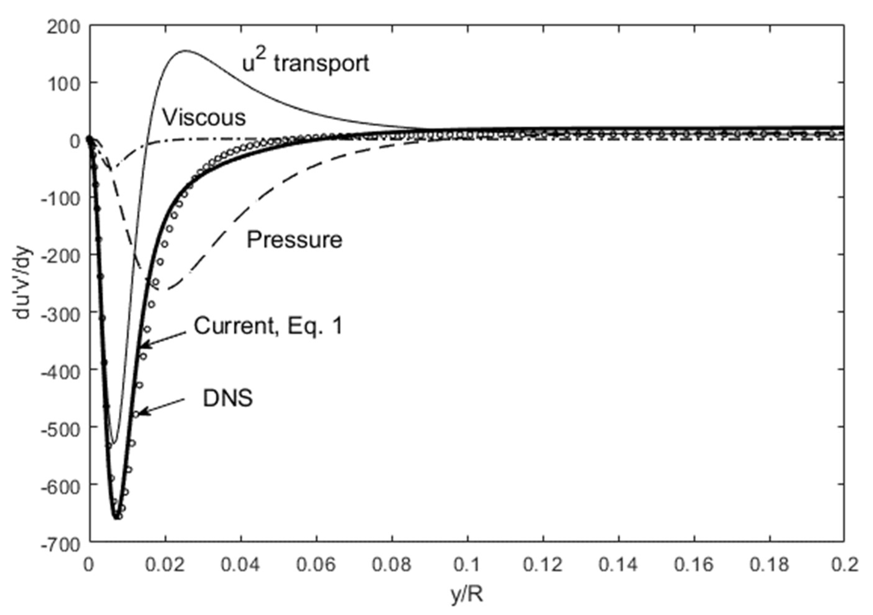
In these equations, the fluctuating terms, u’v’, v’2, etc., are implicitly Reynolds-averaged. The concepts and hypotheses contained in Equations (1)–(3) are described in Lee [17], and also summarized in the next section due to its novelty. These turbulence transport equations, upon validation, furnish a sufficient number of equations to solve for the turbulence variables, when used in conjunction with the Reynolds-averaged Navier–Stokes (RANS) equation(s). Examination of the terms in the Lagrangian turbulence equations illuminates the subtle but intuitive dynamics for the momentum and energy transport. Equation (1), as an example, depicts the Reynolds shear stress as the net lateral transport of the turbulence momentum to balance out the streamwise flux, pressure and viscous forces. The agreement with the DNS data [8] for u’v’ gradient, when computed with Equation (1), is quite good as exemplified in Figure 1, and confirms the simple Lagrangian momentum balance. This is in contrast to the Eulerian models requiring several layers of adjusted relationships to the mean variables. In the Lagrangian perspective, momentum conservation holds in any non-inertial coordinate frame (the Galilean invariance) and the principle of relative motion removes most of the complex coupling with the mean components, leaving bare the core dynamics of turbulence fluctuating variables. In place of unproven proportionality to the mean velocities, relating one fluctuating component to another makes far more dynamical sense.
The equation set, Equations (1)–(3), is an assertion of the basic conservation principles (of momentum and energy) through a Lagrangian perspective, to address the turbulence problem. Another example is the use of the Second Law (of thermodynamics) in the form of maximum entropy principle, to arrive at a lognormal class of turbulence energy spectra [18,19]. The Second Law is also applicable for the uniqueness of the turbulence structure, as there are many possible solutions that may befit the transport equations, but empirically we know that for a given set of boundary conditions only one observable solution of RANS exists. In this paper, the origin of the turbulence structure is examined, as prescribed by the Lagrangian transport equations, and also a brief exhibition is made of the possible solution method to the Navier–Stokes equation(s). Although the title has limited the scope to wall-bounded flows, the results should be applicable to other types of turbulence, e.g., jet flows [16].
2. Lagrantian Turbulence Transport
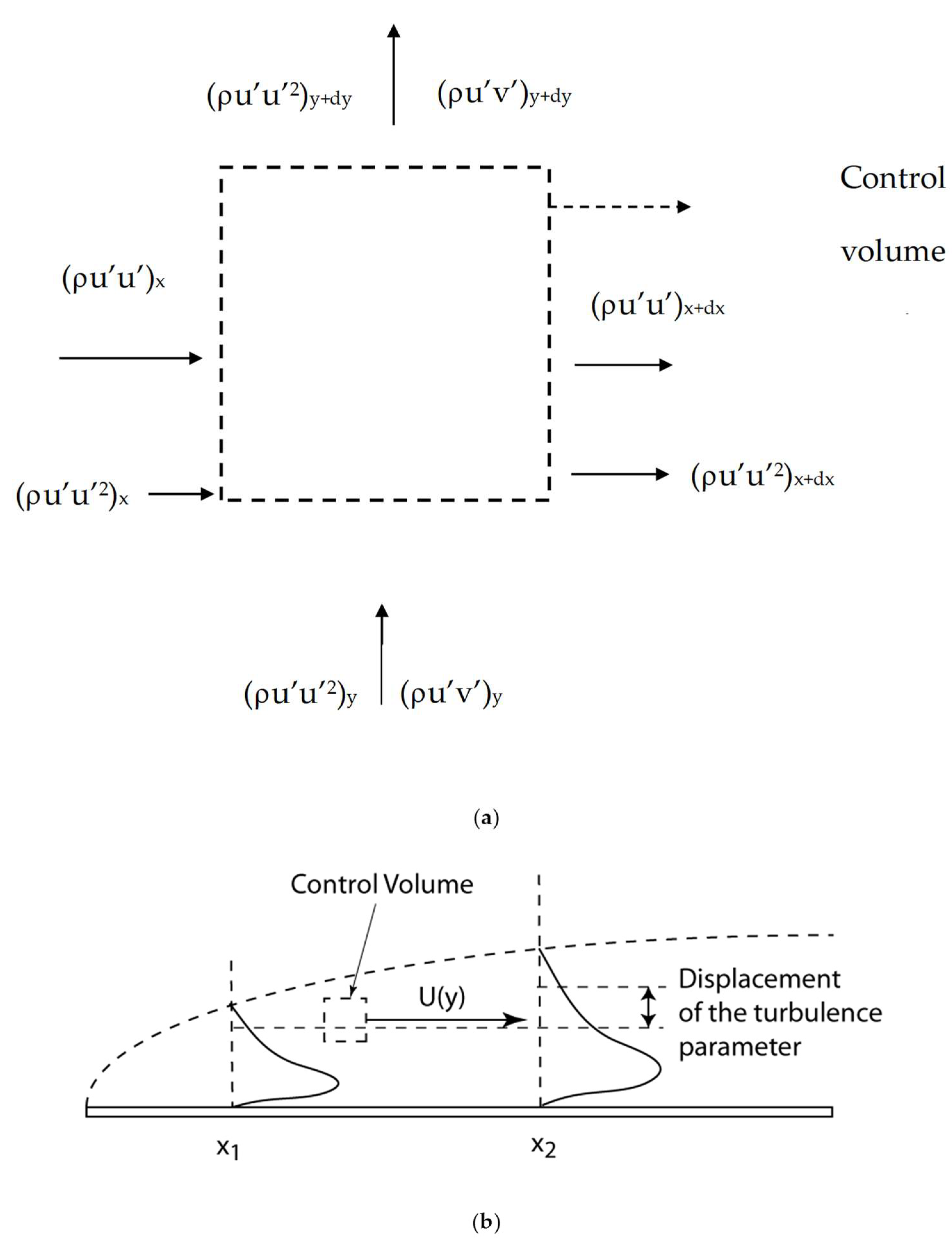
Since this formalism is relatively new, a synopsis of the logic involved is presented herein. For a control volume moving at the local mean velocity, U and V, the effects of turbulence fluctuation components (the Reynolds stress) can in effect be isolated, as depicted in Figure 2. Equation (1) is the transport equation for u’ [14,15,16], where the streamwise flux u’u’ is balanced by the lateral transport, u’v’, pressure and viscous forces. Figure 2a shows similar momentum (v’) and energy transport (u’2), leading to Equations (2) and (3), respectively, while Figure 2b illustrates the displacement transform discussed below.
Due to the displacement effect, d/dx is converted to a d/dy term with the mean velocity as the proportionality constant [14,15,16,17].
C is a constant with the unit ~1/Uref. The +/− sign depends on the flow geometry, i.e., the direction of displacement relative to the reference point. There are no displacement effects for channel flows since the flow is bounded by the walls on both sides. However, we still obtain the above conversion in the spatial gradients using the “probe transform” analysis [17]. Implicit in this transform idea is that the both the vectors (u’, v’) and scalars (pressure, u’2) are displaced or transformed in this manner.
For the triple correlations in u2-transport (energy) equation (Equation (3)), a simple product rule is applied, which has been [16,17] and will be validated from the current results.
Additionally, pressure and its rate of work are written as and , respectively, in Equation (3). These are evidently new and unique concepts, and further details can be found in recent works [16,17]. Some analytics on the turbulence structure, enabled by these dynamical equations, are presented next.
3. Origin of the Turbulence Structure
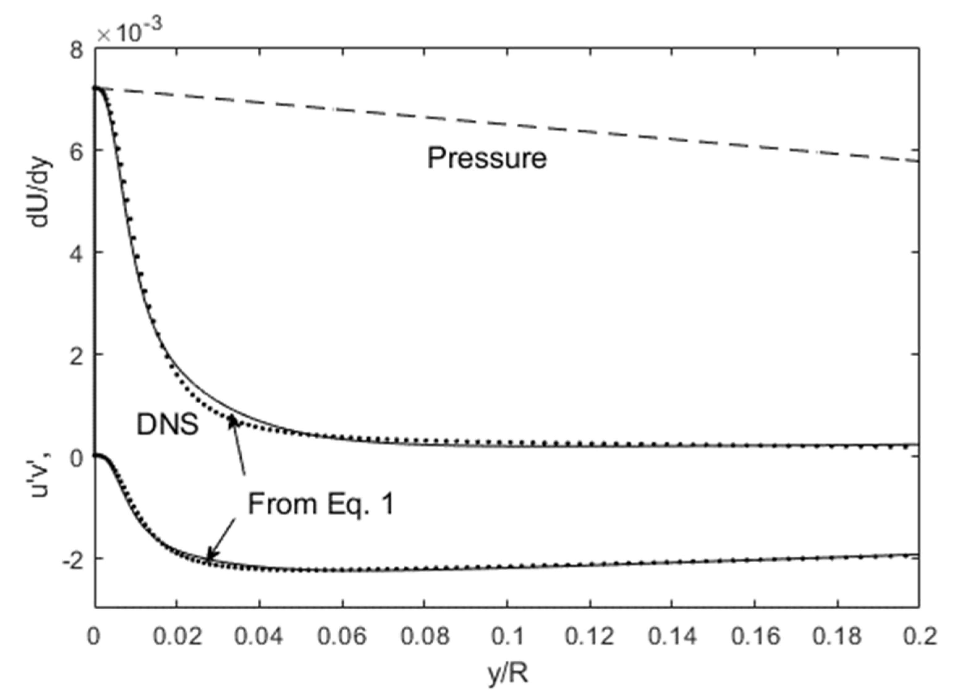
It is quite well known that the mean velocity profile in channel flows arises due to the mean momentum balance between the Reynolds shear stress, viscous, and pressure forces, [20], as described by RANS (Equation (6)) for channel flows. If Equation (6) is integrated once, we obtain the mean velocity gradient (Equation (7)). Thus, Equation (7) can be used along with its plot (Figure 3), as a starting viewpoint.
Individual terms in Equation (7) (mean velocity gradient, Reynolds stress and pressure force) are plotted in Figure 3. Let us focus on the near-wall region (y/R < 0.2) for close inspection and comparison with DNS data for Reλ = 1000 from Graham et al. [8], shown in dot symbols. The turbulence dynamics can be ascertained by substituting into Equation (7) the Reynolds shear stress (u’v’) obtained from Equation (1). For example, inputting u’2, v’2 and U from the DNS data on the right-hand side (RHS) of Equation (1) leads to our own version of d(u’v’)/dy. Then, numerical integration yields u’v’ itself, as plotted in Figure 3. Then, this u’v’ yields dU/dy through Equation (7), both comparable to DNS. We can see that there is a very close agreement with current results of DNS data for the u’v’, and somewhat less so for the dU/dy, possibly due to the division by a small viscosity. Nonetheless, dU/dy computed using u’v’ from Equation (1) has sufficient accuracy to reproduce the mean velocity profile, when integrated once more, because it has all the structural features such as the initial mild slope in the near wall region (y/d < 0.004) and then the sharp descent shortly afterward. The gradient transitions to a small slope between y/d + 0.02 to 0.05. These aspects of dU/dy will result in the flattened velocity profile in channel and other wall-bounded flows.
The first question that arises is: what are the origins of these features in dU/dy? It is evidently from the Reynolds shear stress profile [20], which in turn owes to the d(u’v’)/dy shown earlier in Figure 1. In that figure, u’2-transport term, −C11Udu’2/dy in Equation (1), has a sharp negative peak near the wall (y/R ~ 0.01), while the viscous stress near the wall adds to this negativity. This is the reason the Reynolds shear stress descends rapidly to its minimum near the wall with an inflection at y/R ~ 0.01. This negative plateau occurs y/R ~ 0.05 since that is approximately the location where d(u’v’)/dy → 0 in Figure 1. The pressure force term in Equation (1) subtracts from the u’2-transport term to keep this positive slope small. Thus, from the Lagrangian perspective, the negative peak in the Reynolds shear stress near the wall is due to the momentum balance between streamwise (u’2) and cross-stream (u’v’) momentum fluxes, with the pressure force modifying this x-momentum. Reynolds shear stress is the cross-stream momentum flux to balance the large streamwise flux of u’. In short, tracking the terms in Equation (1) allows us to predict the dU/dy trajectory in Figure 3.
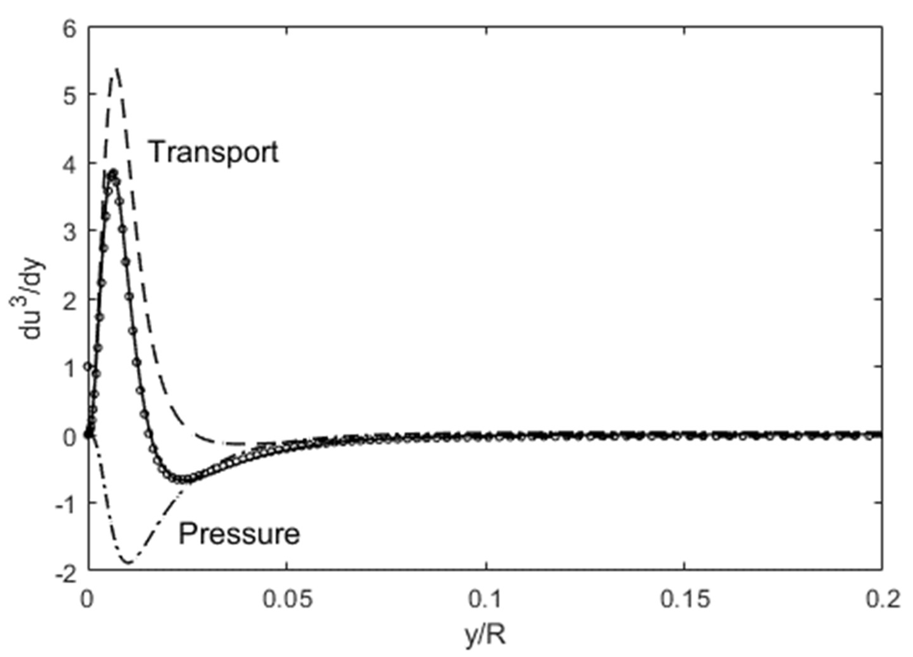
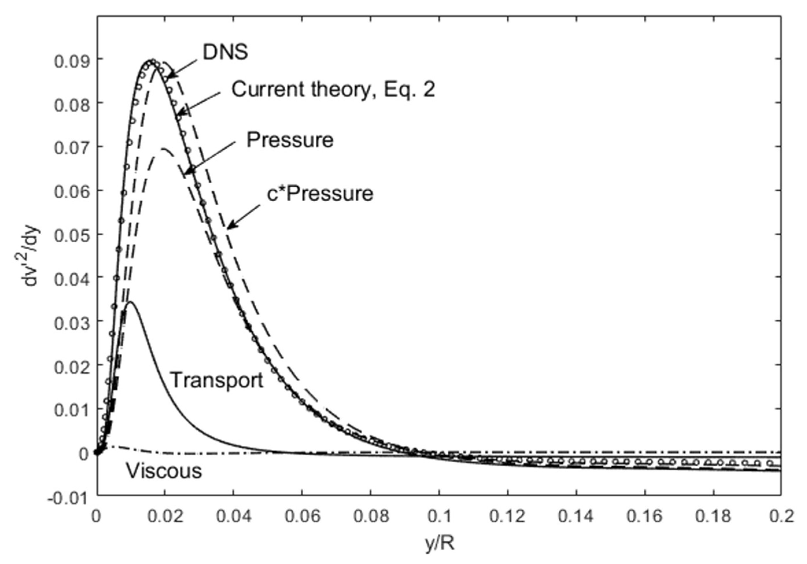
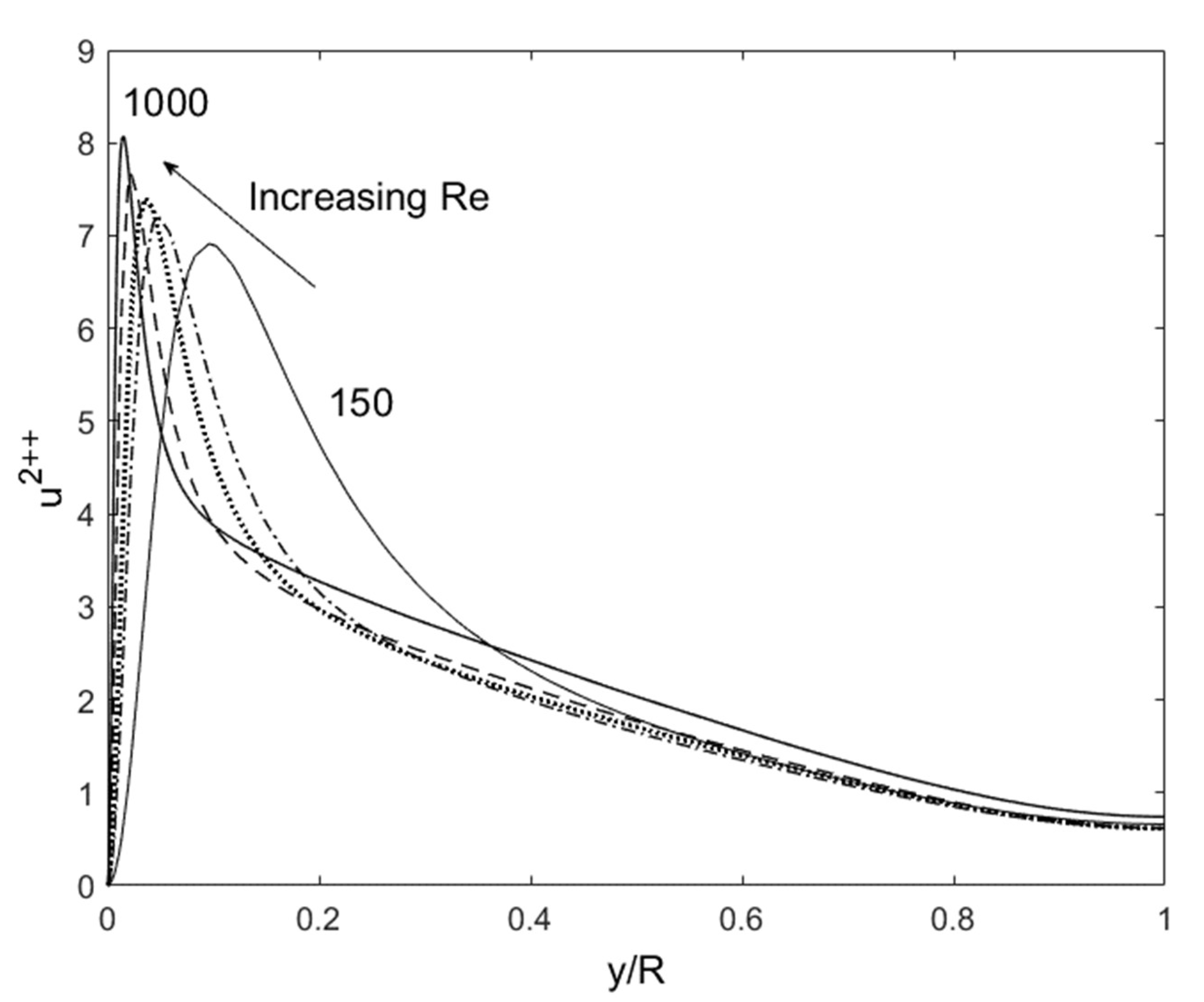
This naturally leads to the next question: what brings forth the structure for x-momentum, u’, or its flux u’2? This momentum component is typically expressed through its kinetic energy manifestation, <u’2> = (u’rms)2. Equation (3) is the Lagrangian transport equation for the u’2 flux, or u’3 = (u’rms)3, which consists of lateral flux of u’2, pressure work, and viscous dissipation term. Figure 4 shows the comparison of Equation (3) with DNS data [8] for du’3/dy, computed as d(u’2)3/2/dy. Again, DNS data for u’v’, v’2 are input on the RHS of Equation (3), to come up with our own “mix” for du’3/dy, and plotted in Figure 4, to validate the Lagrangian energy balance. The budget terms, consisting mainly of lateral flux and pressure work add to a nearly perfect match with DNS data, in spite of and justifying the fact that the viscous term was omitted due to its small magnitude. Thus, Equation (3) depicts the Lagrangian transport for u’2, as validated with DNS data, and presents us with a dynamical picture wherein u’2 is transported laterally by v’, while some of that energy is expended through pressure work (negative). The lateral transport is compacted toward the wall, and this causes a very sharp peak there. This peak then undergoes a gradual decline to the centerline boundary condition, as observed in wall-bounded flows. Notice that most of the action is over by y/R = 0.05 at this Reynolds number, with only a small residual negative slope beyond that. An alternative entropic reason for the u’2 profile taking on a sharp-peak structure near the wall is conjectured further below in the context of Figures 11 and 12.
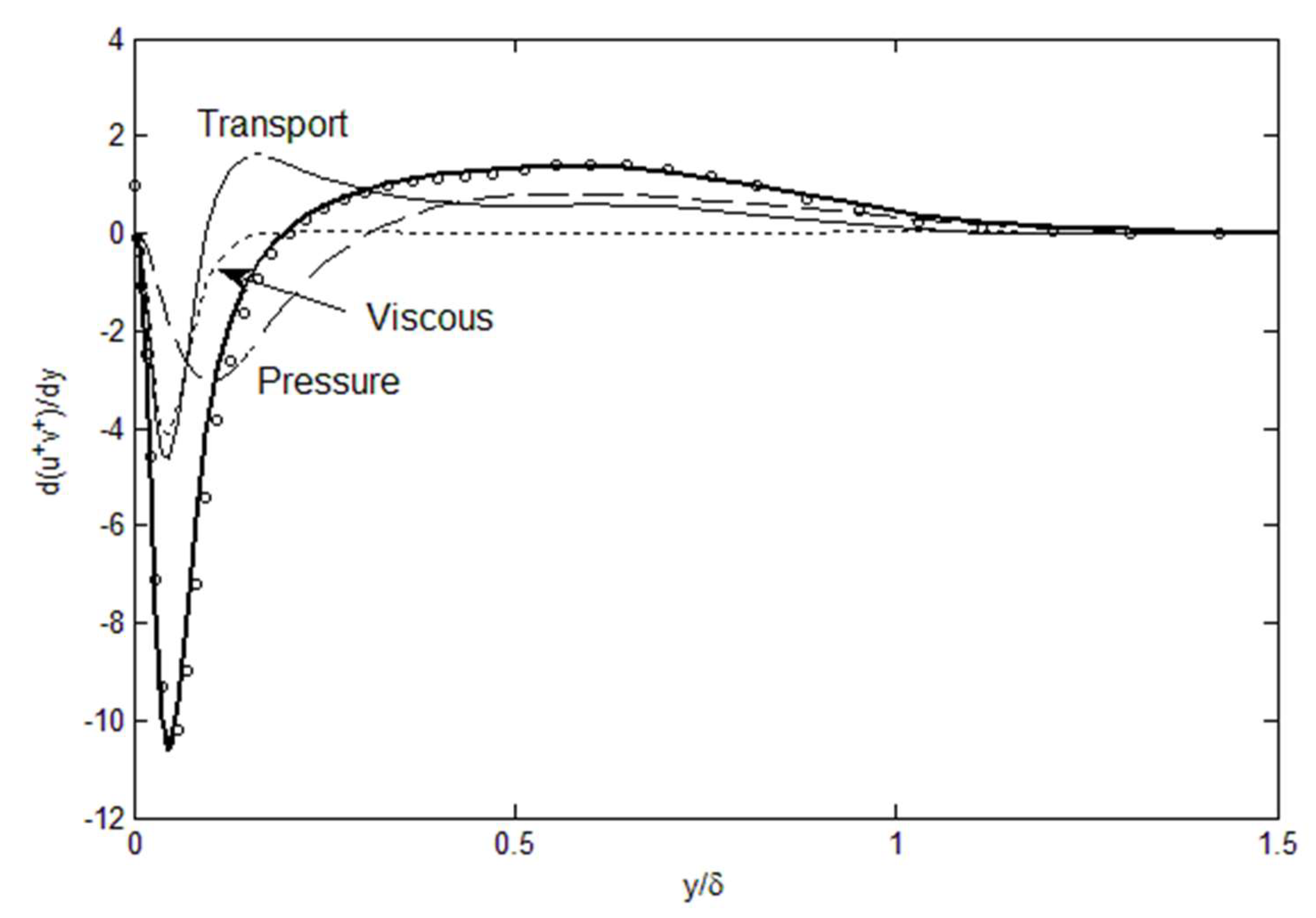
Figure 5 shows a similar confirmation of the Lagrangian momentum balance for v’ through dv’2/dy. Sub-components (RHS of Equation (2)) of the v’-momentum balance have also been plotted. The agreement with Equation (2) is nearly exact till y/R ~ 0.1. Although the negative slope is slightly less than DNS beyond y/R = 0.1, it can be corrected by enforcing the centerline or the total v’2 content boundary condition. It is usually the near-wall behavior that is more complex and difficult to predict. The triad of forces, u’v’-transport, pressure and viscous, conspires intricately to cause the v’2 profile near the wall, in agreement with DNS [8]. It is also interesting to note that the pressure term is the most significant, which would represent a feedback mechanism to outline the v’2 distribution in wall-bounded flows. When we use P = −ρv’2, the role of v’2 is quite significant as it modifies the turbulence structure, and this will be pronouncedly manifest in boundary layer flows as well, discussed later. For the v’-momentum, the moving control volume is subject to shifted gradients in the lateral profiles (see Figure 1) so that the C22U term is again factored to the dP/dy in Equation (2), in order to account for this displacement effect.
Although the above structural questions are posed in sequence, Equations (1)–(3) contain coupling between the turbulence variables, u’2, v’2 and u’v’, so the logical train could have been initiated with any one of these three components. The important conclusion is that the Lagrangian transport equations furnish the inter-relationships between the turbulence variables, so that we can obtain a succinct view of the underlying dynamics, and also compute and reconstruct the variables directly. Let us see what this new perspective reveals when we examine boundary layer flows over a flat plate. The same set of transport equations holds for turbulent flows in various geometries [16,17], and Figure 6 is a plot exhibiting the Reynolds stress gradient budget, for flow over a flat plate with a zero pressure gradient (ZPG). The DNS data (symbols) from Spalart [5] for Reτ = 670 are used for comparison. We can again see in Figure 6 that the contribution of the viscous term to the Reynolds stress gradient is relatively small and limited to the near-wall region. The u’2 (longitudinal transport) term has the largest effect, particularly near the wall due to its steep gradient, first upward then down. In the current Lagrangian analysis, the pressure force is manifest in the cross-stream direction due to the displacement effect, i.e., movement of the control volume through the displaced layers will cause a small but finite pressure imbalance in the y-direction. In Equation (1), this is expressed through dP/dx → −CUdv’2/dy where the mean pressure is approximated as −ρv2 [21]. These three terms all add up to the Reynolds stress gradient, nearly precisely, as shown in Figure 6. We observe that the Reynolds shear stress is structurally similar to channel flows, but now contains a pronounced positive slope (bulge) as one moves away from the wall. This bulge is induced by the combination of the transport and pressure terms. This has some consequences if the flow is subject to adverse pressure gradients (APG), discussed next.
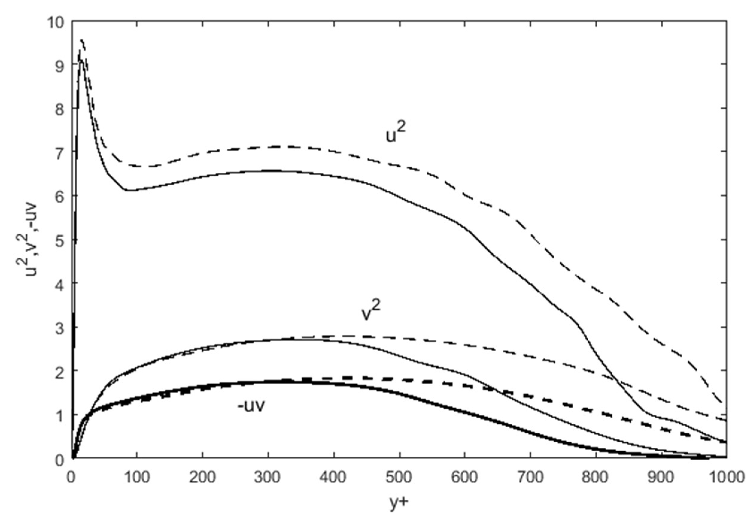
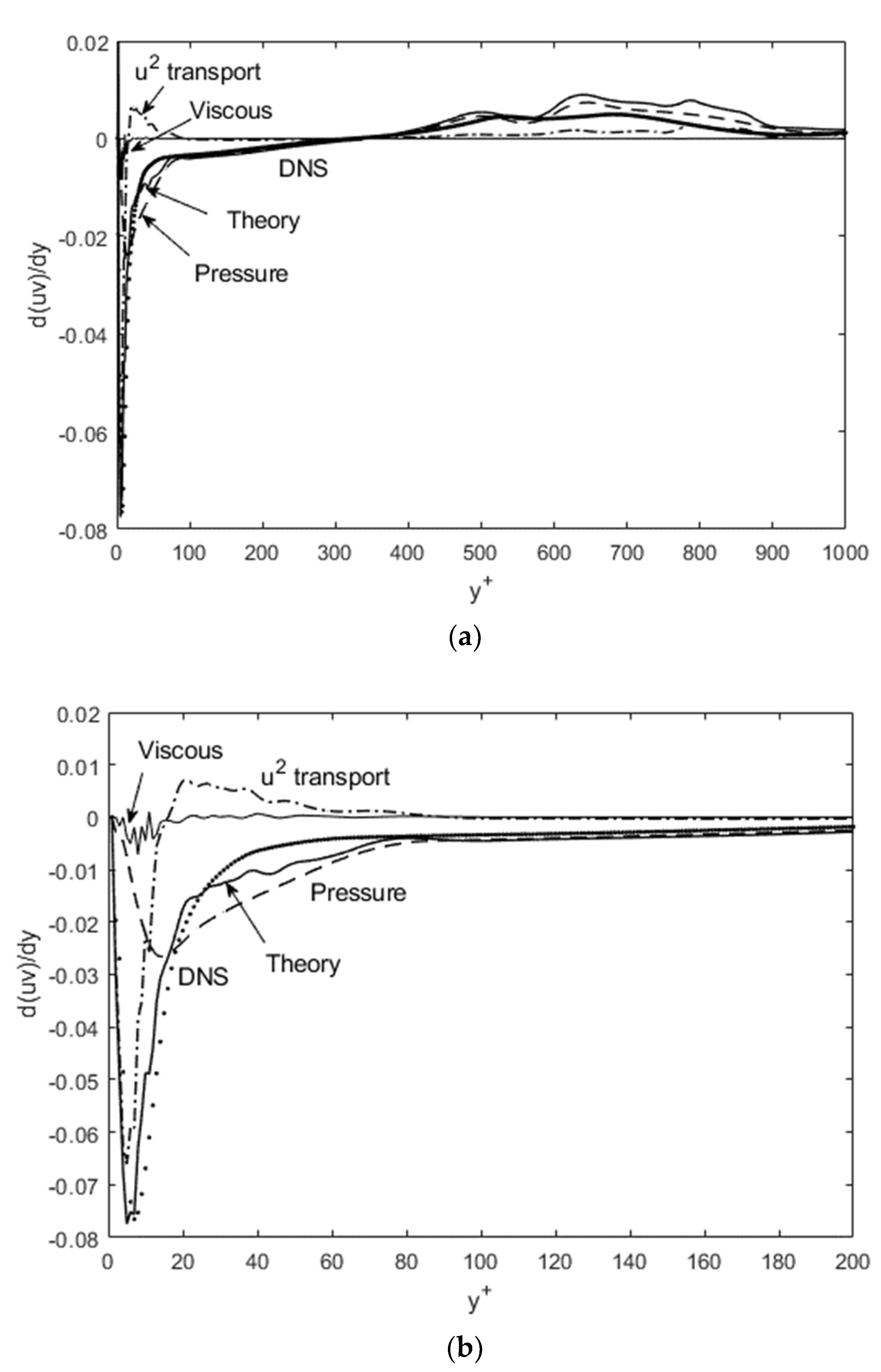
The alterations of the basic turbulence parameters, when an adverse pressure gradient (APG) is applied for the boundary layer flow, can be visualized by plotting u’2 and v’2 from DNS data [6] in Figure 7. Relative to ZPG, both u’2 and v’2 profiles contain pronounced protuberance in the mid-layer region. In ZPG, the u’2 and v’2 have monotonic decreases after the near-wall peak. Equation (1) predicts that these undulations between y+ ~ 500 to 900 will lead to similar features in the Reynolds shear stress in the opposite direction (sign). The individual terms in Equation (1) for APG are again plotted, and compared with the sum with DNS data, in Figure 8. The viscous term is included, in spite of its numerical perturbations, to illustrate its impact. It does add to the overall momentum balance, but higher-definition data (than what was available to us) is required to compute the second gradient accurately.
Figure 8a shows the entire d(u’v’)/dy profile across the boundary layer, while Figure 8b zooms in on the near-wall region for a closer inspection. The overall agreement between Equation (1) and DNS results is good across the boundary layer; however, the gradients are not entirely smooth and there are some deviations. This includes the undulations away from the wall, which is mimicked but not exactly followed by Equation (1). This is attributed to the tracing of the DNS data from Kitsios et al. [6], leading to some errors when taking the gradient of the transcribed data. This kind of numerical differentiation error is present in Figure 8b as well, where a close inspection of the near-wall region again shows that Equation (1) tracks the DNS data reasonably well, albeit with some small spikes and undulations. At the inflection point (y+~40), there is some deviation from DNS data. Nonetheless, the overall structure and origin of the Reynolds shear stress are captured by Equation (1), providing further ascertainment in a different flow geometry.
As for the features in u’2 and v’2 profiles translating to d(u’v’)/dy, the protuberance after the near-wall peak in Figure 8 will lead to small positive then negative slopes for du’2/dy and dv’2/dy. The u2-transport and pressure terms (the first and second on RHS) of Equation (1) point toward d(u’v’)/dy having negative slopes for 100 < y+ <~ 380) then positive slopes for ~380 < y+ < 900. Since the u’2-transport effect is quite strong at y+ < 100, while it is the pressure force that dictates the momentum balance afterward, the adverse-pressure gradient effect is manifest through the pressure term and onto d(u’v’)/dy during ~380 < y+ < 900. These distinct features in the Reynolds shear stress in APG result in the mean velocity profile exhibiting different slopes (in comparison to ZPG) in the same region (~380 < y+ < 900) [6].
In summary, the transport equation set (Equations (1)–(3)) is based on the fundamental fluid physics of momentum and energy conservation in a specific moving coordinate frame, and provides intuitive, dynamical explanations of the features observed in turbulence structures. Eulerian versions of the same phenomena tend to hide the underlying dynamics, first simply due to the large number of inter-correlated source and sink terms. Secondly, when layers of complex ad hoc models, e.g., mean gradient transport, are introduced to the pure transport equations, then the basic fluid physics of turbulence tend to become obscured or at times abandoned. As validated, current set of turbulence transport equations provide a clear and succinct view of the turbulence physics. In addition, it points to a viable solution method, as there is now a sufficient number of equations (Equations (1)–(3) and (6)) for the unknown turbulence variables.
4. Implications toward Computability of Turbulent Flows
The transport expressions for u’v’, v’2, and u’2 (Equations (1)–(3)) along with RANS (Equation (6)) for U furnish an inter-coupled but complete set of equations to solve for these variables. The full solution algorithm is deferred to a later study, as we are first interested in the solvability/computability of RANS for wall-bounded flows without modeling or direct numerical simulations. In order to illustrate how the mean velocity profile can be computed from RANS, the following steps are utilized, similar to a previous work [16]:
- Start from initial estimated test functions for u’2, v’2, and U.
- Using Equation (1), compute then integrate d(u’v’)/dy to find u’v’.
- Use u’v’ in Equation (7), to compute and integrate dU/dy to find U.
- Update v’2 using the computed d(u’v’)/dy and U in Equation (2).
- With the computed u’v’, U, and updated v’2, update u’2 using Equation (3).
- Repeat (iterate) until convergence.
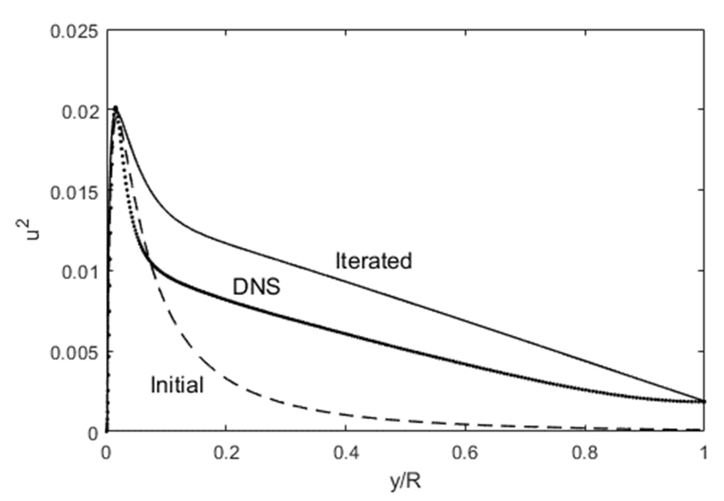
Figure 9 and Figure 10 show the result of running the above routine. The starting test functions for u’2 and v’2 are lognormal functions, while we expedite the numerics with an initial U = y1/n, where n = 7. All the test functions, including this U, are updated using Equations (1)–(3) during the iteration. To facilitate convergence, we also use a y m type of function on the “backside” (y/R = 0.5~1) for u’2, which ensures that the boundary conditions are enforced both at y/R = 0 and 1. After just one iteration, a reasonable u’2 profile starts to emerge, after again setting u’2 = (u’2)y/R = 1 at y/R = 1 (the centerline boundary condition), in Figure 9. (u’2) y/R = 1 can be obtained from DNS data, or estimated from E (Equation (8) below).
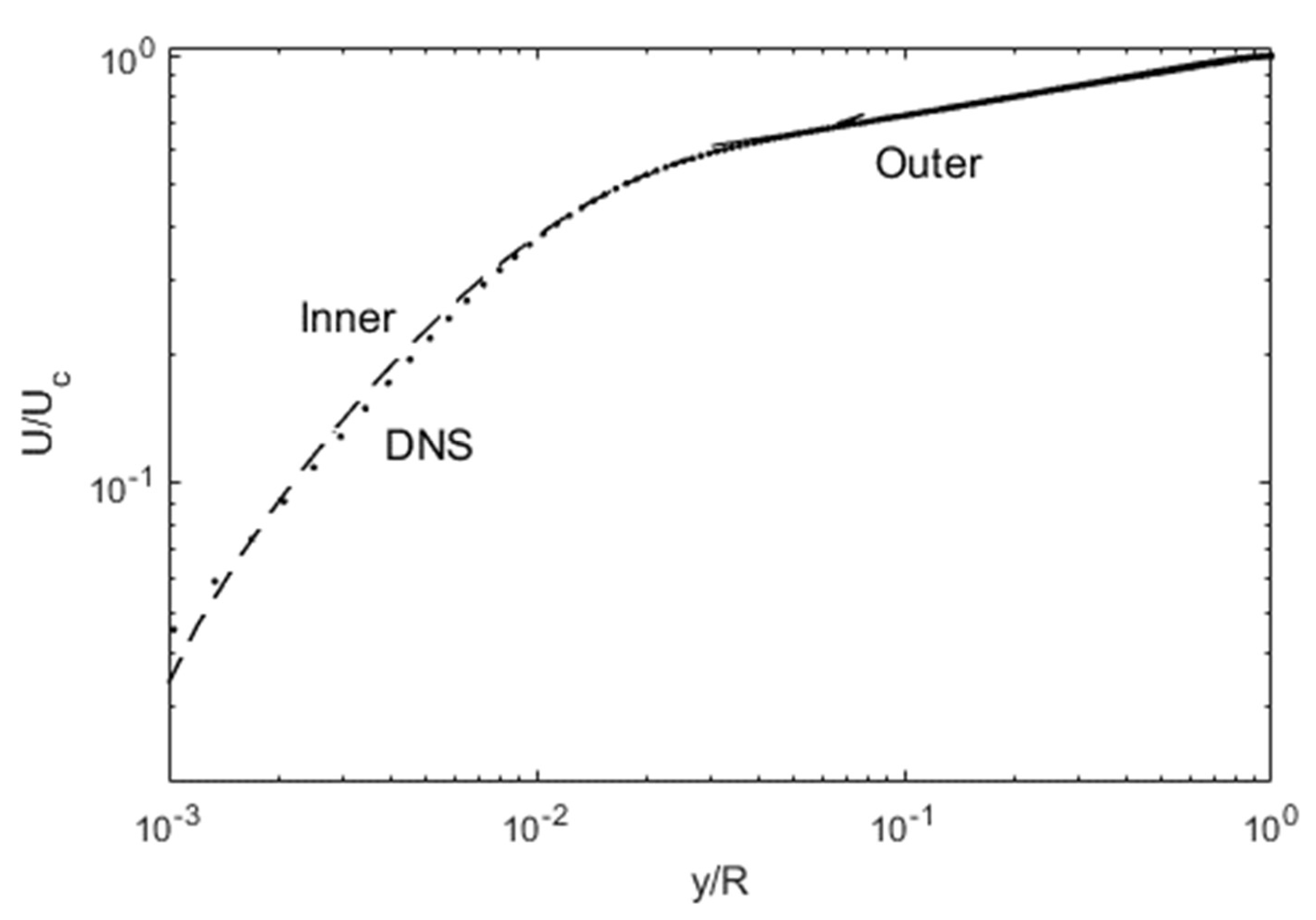
Reynolds shear stress is obtained from Step 2, which leads to the mean velocity profile in Step 3. This single-iteration result for the mean velocity shown in Figure 10 is quite close to the DNS data. In order to circumvent integration errors in the mid-layer, dU/dy is integrated from both y/R = 0 and 1 until the solutions intersect (at about y/R = 0.6). Outer solution has a small slope, fairly close to the often-used approximation, U~y1/n [21]. The inner solution advances to this “power-law” region, all the while tracking the DNS data closely. An important point to be made here is that the mean velocity profile in Figure 10 satisfy the RANS (Equation (6)), along with other transport equations that are associated with or needed to solve it: Equation (1) for the Reynolds shear stress, u’v’ that goes in Equation (6) explicitly, and then Equations (2) and (3) for v’2 and u’2, respectively. Thus, a U-profile that satisfies Equations (1)–(3) implicitly and also Equation (6) explicitly, is a valid solution to RANS. However, is it a unique solution?
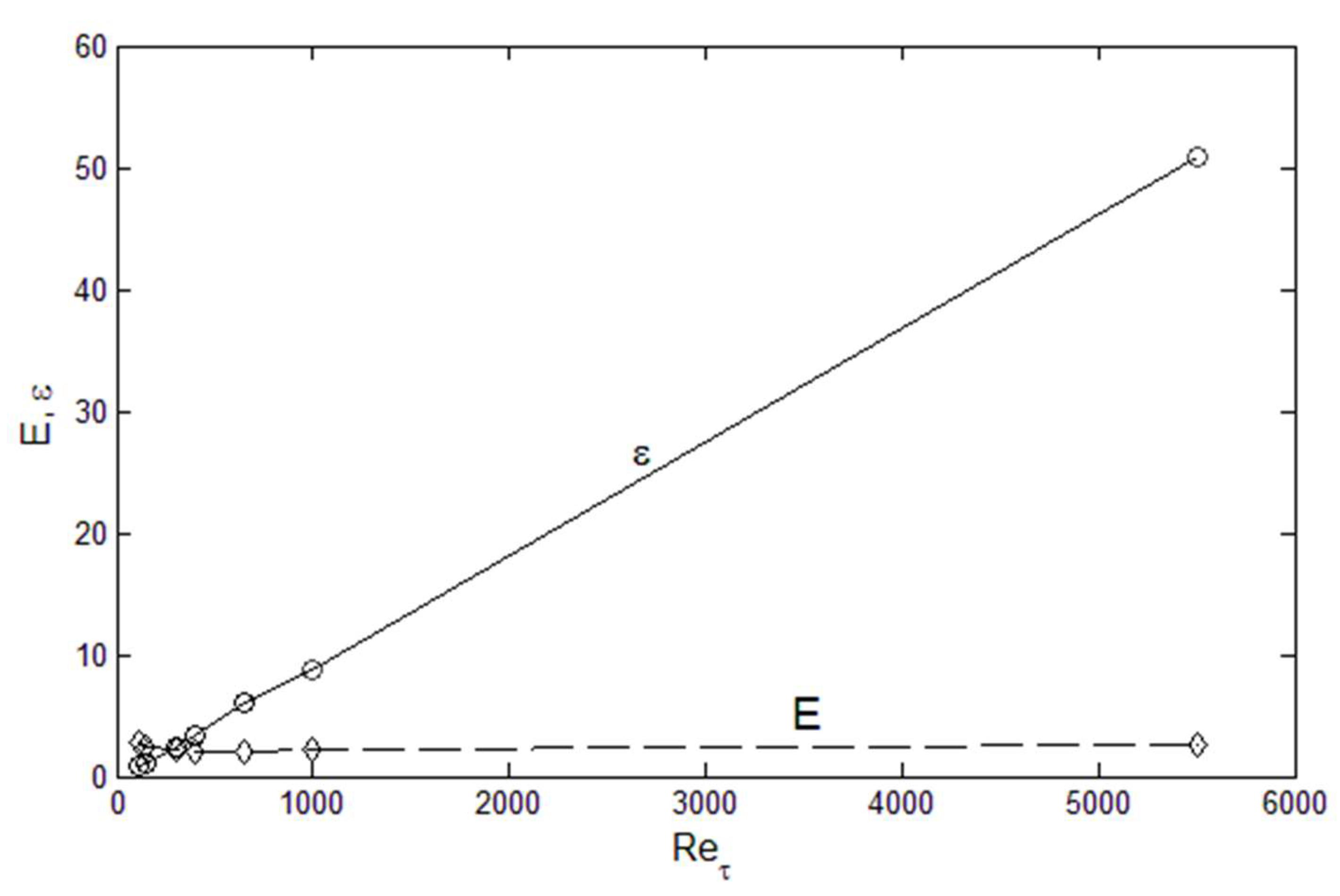
The answer is that there are different solutions to RANS depending on the Reynolds number. Even for high Reynolds numbers, fully turbulent flows and minute differences are observable in the mean velocity, and there are substantial changes in the u’2 profiles as the Reynolds number increases. Therefore, the solution to RANS is unique only to a particular Reynolds number: an obvious point, but it leads to a somewhat philosophical query of what causes the shift in the solution as a function of the Reynolds number. As we have seen thus far, the mean velocity profile from RANS is the result of turbulence transport of u’v’, u’2 and v’2. Then, the specificity of these variables at a given Reynolds number is inevitably connected to the uniqueness of solution to RANS. To explain this connection, we can look at the energy (E) and dissipation (ε) content of the flow, as shown in Figure 11, where the definitions are written in Equations (8) and (9).
In Figure 11, we see that E is all but constant, when properly normalized by the friction velocity (u’+ = u’/Uτ where Uτ is the friction velocity). For the dissipation, ε, there is a linear dependence on the Reτ. Therefore, for a fixed normalized energy content, E, dissipation increases because the relative influence of viscosity is reduced at higher Reynolds numbers. If we invoke the Second Law (the entropy principle), the u’+2 distribution distorts itself to achieve the maximum dissipation until the restraining force of viscosity imposes its upper limit, all the while obeying the physical constraints of continuity, smoothness, E = constant, and boundary conditions at the wall and the centerline (see Figure 12). The maximum distortion, which may be interpreted as turbulence entropy, is set by ε as a function of Reτ. Therefore, the origin of the uniqueness and structure of the solutions to RANS can be said to be due to the Second Law. After this manifestation, other turbulence variables organize themselves according to the momentum (Equations (1), (2) and (6)) and energy (Equation (3)) conservation principles.
5. Conclusions
A symmetric set of gradient expressions for the Reynolds stress tensor components is obtained from the Lagrangian transport analysis of turbulence. In this perspective, the turbulence structure in wall-bounded flows can be viewed as an inter-play of a small number of momentum or energy terms: transport, pressure and viscous. Using this formalism, features of the turbulent flow can be understood and reconstructed in simple dynamical relationships, as demonstrated here for channel and boundary layer flows (with and without pressure gradients). This set of transport expressions furnish a sufficient number of equations, along with RANS, to iteratively solve for the mean velocity in turbulent channel flows. The uniqueness and computability of such solutions at given Reynolds numbers are briefly philosophized, from the Second Law perspective.
The above perspectives offer a complete departure from the existing entrenched lines of thought such as mean-gradient transport, attached-eddy [1,12], and asymptotic-layer [13] models. Instead, coordinate-shifted momentum and energy analyses are applied to generate a closed set of transport equations for the Reynolds stress components. Thus far, comparisons with experimental and DNS data support the hypotheses and the theoretical framework. Thus far, the validations have been limited and carried out in canonical geometries, swirl and adverse-pressure gradient flows, as discussed above. If further confirmations are made in fully three dimensional flows, a revolutionary method to solve for turbulent flows may be enabled analytically and computationally.
Funding
This research was funded in part by SRP, Arizona.
Institutional Review Board Statement
Not applicable.
Informed Consent Statement
Not applicable.
Data Availability Statement
The data used in this study are available from open sources.
Conflicts of Interest
The author declares no conflict of interest.
References
- Adrian, R.J. Closing in on models of wall turbulence. Science 2010, 329, 155–156. [Google Scholar] [CrossRef] [PubMed]
- Marusic, I.; McKeon, B.J.; Monkewitz, P.A.; Nagib, H.M.; Smits, A.J.; Sreenivasan, K.R. Wall-bounded turbulent flows at high Reynolds numbers: Recent advances and key issues. Phys. Fluids 2010, 22, 065103. [Google Scholar] [CrossRef]
- Moin, P.; Mahesh, K. Direct numerical simulation: A tool in turbulence research. Annu. Rev. Fluid Mech. 1998, 30, 539–578. [Google Scholar] [CrossRef] [Green Version]
- Mansour, N.N.; Kim, J.; Moin, P. Reynolds-stress and dissipation-rate budgets in a turbulent channel flow. J. Fluid Mech. 1998, 194, 15–44. [Google Scholar] [CrossRef] [Green Version]
- Spalart, P.R. Direct simulation of a turbulent boundary layer up to Re = 1410. J. Fluid Mech. 1988, 187, 61–77. [Google Scholar] [CrossRef]
- Kitsios, V.; Atkinson, C.; Sillero, J.A.; Borrell, G.; Gungor, A.G.; Jiménez, J.; Soria, J. Direct numerical simulation of a self-similar adverse pressure gradient turbulent boundary layer. Int. J. Heat Fluid Flow 2016, 61, 129–136. [Google Scholar] [CrossRef] [Green Version]
- Nygard, F.; Andersson, H. DNS of swirling turbulent pipe flow. Int. J. Numer. Methods Fluids 2009, 64, 945–972. [Google Scholar] [CrossRef]
- Graham, J.; Kanov, K.; Yang, X.I.A.; Lee, M.K.; Malaya, N.; Lalescu, C.C.; Burns, R.; Eyink, G.; Szalay, A.; Moser, R.D.; et al. A Web Services-accessible database of turbulent channel flow and its use for testing a new integral wall model for LES. J. Turbul. 2016, 17, 181–215. [Google Scholar] [CrossRef]
- Na, Y.; Hanratty, T.; Liu, T.J. The use of DNS to define stress producing events for turbulent flow over a smooth wall. Flow Turbul. Combust. 2001, 66, 495–512. [Google Scholar] [CrossRef]
- Moser, R.D.; Kim, J.; Mansour, N.N. Direct numerical simulation of turbulent channel flow up to Reτ = 590. Phys. Fluids 1999, 11, 943–945. [Google Scholar] [CrossRef]
- Iwamoto, K.; Sasaki, Y.; Nobuhide, K. Reynolds number effects on wall turbulence: Toward effective feedback control. Int. J. Heat Fluid Flows 2002, 23, 678–689. [Google Scholar] [CrossRef]
- Marusic, I.; Monty, J.P. Attached eddy model of wall turbulence. Annu. Rev. Fluid Mech. 2019, 51, 49–74. [Google Scholar] [CrossRef]
- Klewicski, J.; Fife, P.; Wei, T. On the logarithmic mean profile. J. Fluid Mech. 2009, 638, 73–93. [Google Scholar] [CrossRef]
- Lee, T.-W. Reynolds stress in turbulent flows from a Lagrangian perspective. J. Phys. Commun. 2018, 2, 055027. [Google Scholar] [CrossRef] [Green Version]
- Lee, T.-W.; Park, J.E. Integral Formula for Determination of the Reynolds Stress in Canonical Flow Geometries. In Progress in Turbulence VII; Orlu, R., Talamelli, A., Oberlack, M., Peinke, J., Eds.; Springer: Cham, Switzerland, 2017; pp. 147–152. [Google Scholar]
- Lee, T.-W. Lagrangian Transport Equations and an Iterative Solution Method for Turbulent Jet Flows. Phys. D 2020, 403, 132333. [Google Scholar] [CrossRef]
- Lee, T.-W. Dissipation scaling and structural order in turbulent channel flows. Phys. Fluids 2021, 33, 055105. [Google Scholar] [CrossRef]
- Lee, T.-W. Lognormality in turbulence energy spectra. Entropy 2020, 22, 669. [Google Scholar] [CrossRef] [PubMed]
- Lee, T.-W. Scaling of the maximum-entropy turbulence energy spectra. Eur. J. Mech. B/Fluids 2021, 87, 128–134. [Google Scholar] [CrossRef]
- Panton, R.L. Incompressible Flow, 4th ed.; Wiley: Hoboken, NJ, USA, 2013. [Google Scholar]
- Pope, S.B. Turbulent Flows; Cambridge University Press: Cambridge, UK, 2012. [Google Scholar]
Figure 1.
The u’-momentum budget for the Reynolds shear stress gradient (Equation (1)), and comparison with the DNS data [8].
Figure 1.
The u’-momentum budget for the Reynolds shear stress gradient (Equation (1)), and comparison with the DNS data [8].

Figure 2.
Schematics of the dynamics contained in the Lagrangian turbulence transport: (a) y-momentum (v’) and longitudinal kinetic energy balance (u’2) following a control volume, moving at the local mean velocity; (b) the displacement concept leading to d/dx → d/dy transform.
Figure 2.
Schematics of the dynamics contained in the Lagrangian turbulence transport: (a) y-momentum (v’) and longitudinal kinetic energy balance (u’2) following a control volume, moving at the local mean velocity; (b) the displacement concept leading to d/dx → d/dy transform.

Figure 3.
The Reynolds stress (Equation (1) integrated) and the mean velocity gradient (Equation (7) with the integrated u’v’), as compared with DNS data [8] plotted as dot symbols. y is normalized by the channel half-width (R).
Figure 3.
The Reynolds stress (Equation (1) integrated) and the mean velocity gradient (Equation (7) with the integrated u’v’), as compared with DNS data [8] plotted as dot symbols. y is normalized by the channel half-width (R).

Figure 4.
The budget for u’2 kinetic energy (Equation (3)), and comparison with DNS data [8] plotted as symbols.
Figure 4.
The budget for u’2 kinetic energy (Equation (3)), and comparison with DNS data [8] plotted as symbols.

Figure 5.
The budget for v’-momentum. Again, DNS data [8] is used for confirmation of Equation (2).
Figure 5.
The budget for v’-momentum. Again, DNS data [8] is used for confirmation of Equation (2).

Figure 6.
Reynolds stress gradient budget for flow over a flat plate at zero pressure gradient. DNS data (symbol) is from Spalart [5]. Solid line is from Equation (1).
Figure 6.
Reynolds stress gradient budget for flow over a flat plate at zero pressure gradient. DNS data (symbol) is from Spalart [5]. Solid line is from Equation (1).

Figure 7.
Basic turbulence variables, −u’v’, u’2, and v’2, from DNS data of Kitsios et al. [6]. Re = 3500 (solid lines) and Re = 4800 (dashed lines).
Figure 7.
Basic turbulence variables, −u’v’, u’2, and v’2, from DNS data of Kitsios et al. [6]. Re = 3500 (solid lines) and Re = 4800 (dashed lines).

Figure 8.
Reynolds stress gradient budget for flow over a flat plate with adverse pressure gradient. DNS data (dot symbols) is from Kitsios et al. [6] at Re = 3500; (b) contains the same data as (a), except zoomed on the near-wall region.
Figure 8.
Reynolds stress gradient budget for flow over a flat plate with adverse pressure gradient. DNS data (dot symbols) is from Kitsios et al. [6] at Re = 3500; (b) contains the same data as (a), except zoomed on the near-wall region.

Figure 9.
Turbulence kinetic energy, u2, iterated using Equations (1)–(3) and (7).

Figure 10.
Normalized mean velocity profile, iterated from Equations (1)–(3) and (6).

Figure 11.
The total turbulence kinetic energy and dissipation as a function of Reynolds number for channel flows. DNS data are from Iwamoto [11] and Graham et al. [8].


Publisher’s Note: MDPI stays neutral with regard to jurisdictional claims in published maps and institutional affiliations. |
© 2021 by the author. Licensee MDPI, Basel, Switzerland. This article is an open access article distributed under the terms and conditions of the Creative Commons Attribution (CC BY) license (https://creativecommons.org/licenses/by/4.0/).
Share and Cite
MDPI and ACS Style
Lee, T.-W. Origin of the Turbulence Structure in Wall-Bounded Flows, and Implications toward Computability. Fluids 2021, 6, 333. https://0-doi-org.brum.beds.ac.uk/10.3390/fluids6090333
AMA Style
Lee T-W. Origin of the Turbulence Structure in Wall-Bounded Flows, and Implications toward Computability. Fluids. 2021; 6(9):333. https://0-doi-org.brum.beds.ac.uk/10.3390/fluids6090333
Chicago/Turabian StyleLee, T.-W. 2021. "Origin of the Turbulence Structure in Wall-Bounded Flows, and Implications toward Computability" Fluids 6, no. 9: 333. https://0-doi-org.brum.beds.ac.uk/10.3390/fluids6090333