
Application of an Integral Turbulence Model to Close the Model of an Anisotropic Porous Body as Applied to Rod Structures


Institute of Nuclear Physics and Engineering, National Research Nuclear University MEPhI (Moscow Engineering Physics Institute), Kashirskoye Shosse 31, 115409 Moscow, Russia
*
Author to whom correspondence should be addressed.
Fluids 2022, 7(2), 77; https://0-doi-org.brum.beds.ac.uk/10.3390/fluids7020077
Submission received: 30 November 2021
/
Revised: 7 February 2022
/
Accepted: 8 February 2022
/
Published: 14 February 2022
(This article belongs to the Special Issue Stochastic Equations in Fluid Dynamics)
Abstract
:In practice, often devices are ordered rod structures consisting of a large number of rods. Heat exchangers, fuel assemblies of nuclear reactors, and their cores in the case of using caseless assemblies are examples of such devices. Simulation of heat and mass transfer processes in such devices in porous-body approximation can significantly reduce the required resources compared to computational fluid dynamics (CFD) approaches. The paper describes an integral turbulence model developed for defining anisotropic model parameters of a porous body. The parameters of the integral turbulence model were determined by numerical simulations for assemblies of smooth rods, assemblies with spacer grids, and wire-wrapped fuel assemblies. The results of modeling the flow of a liquid metal coolant in an experimental fuel assembly with local blocking of its flow section in anisotropic porous-body approximation using an integral turbulence model are described. The possibility of using the model of an anisotropic porous body with the integral model of turbulence to describe thermal-hydraulic processes during fluid flow in rod structures is confirmed.
1. Introduction
In engineering practice, integral and local approaches are used to simulate thermal-hydraulic processes in the cores of nuclear power plants and other heat-exchange equipment. The integral approach includes sub-channel and porous body models. These models operate with process averaged characteristics. Local models operate with local characteristics and allow one to determine their value at any point in the computational domain. They are implemented in the so-called computational fluid dynamics (CFD) codes. Both approaches are based on the Navier–Stokes (NS) equations, which describe mass and momentum conservation. In addition to those equations, the energy conservation equation is solved.
Sub-channel models operate with averaged characteristics, which are of the main interest in most problems but allow one to determine their value only at the corresponding nodes of the elements into which the computational domain is divided. These methods were developed [1,2] and continue to be used now. A large number of codes have been developed using this approach. The ability to integrate sub-channel and system code in one software product [3], as well as relatively low requirements for computer resources [4], are the advantages of this approach. The main disadvantage of this approach is the need to determine the closing relations, in particular, the coefficients of interchannel mixing ratio, which directly depend on the corresponding geometry and flow regime [3,4,5,6]. These relations are not directly derived from the three-dimensional equations for the flow and should be determined mainly experimentally for similar conditions.
The porous-body model has lower computational costs compared to CFD codes and is comparable to sub-channel models. In contrast to sub-channel models, the closing relations are obtained by averaging three-dimensional equations [7] and have a clear physical meaning; therefore, they are easier to determine, and they work in a wide range of geometric and operating parameters. Closing relationships can be determined using experimental data or CFD simulations. The equations of the porous body model [8] describe the averaged flow parameters that are continuously changing over the entire computational domain. The finite element method (FEM) [9] or the finite volume method (FVM) [10] applied for discretizing the computational domain allows for calculating geometries of arbitrary shape and does not require the use of structured grids, in contrast to the sub-channel approach. This approach allows for a determination of the average parameters at any point in the computational domain.
CFD models use a direct solution of NS equations (DNS approach) or their approximate solution using large eddy simulation (LES), Reynolds-averaged Navier–Stokes (RANS) approaches [11].
The DNS approach requires huge computational resources. It is expected that at the current rate of development of these resources, it will become available for solving problems of flow around a typical civil aircraft or car, with the number of grid nodes and the number of time steps at approximately 1016 and 107.7, respectively, no earlier than 2080 [12].
The LES approach, in which “large vortices” are described accurately, and approximate relations are used for “small” ones, requires noticeably less computational resources compared to the DNS approach [12]. However, the required resources remain very significant, so it is mainly used to validate the results obtained by the RANS approach, as well as to solve problems where the use of the RANS approach leads to incorrect results [12].
The RANS approach is based on the solution of the averaged NS equations and requires the use of semi-empirical turbulence models [12]. Its popularity is due to the relatively low cost of computing resources compared to using LES and even more so DNS approaches. Nevertheless, even using the RANS approach requires a huge amount of computational resources when simulating the core of a nuclear power plant [3]. RANS turbulence models are excellent for modeling fragments of an investigated object [13] to determine the required parameters or to determine the closing relationships of sub-channel models and a porous body model in the absence of experimental data. Also, at the moment, there is a problem with validating the results obtained using CFD codes on full-scale models, such as the reactor core [14].
In this paper, to describe thermo-hydraulic processes, an approach based on the model of an anisotropic porous body is used. The possibility of determining the closing relations of this model using a special integral turbulence model is shown. Calculated relationships are obtained for the parameters of the integral turbulence model for the main types of rod structures used in heat exchange equipment.
2. Anisotropic Porous Body Model
Hereinafter, the following notation is used:
—variable; —time-averaged variable value; —volume-averaged variable value; —fluid volume-averaged variable value; and —deviation from the value of the fluid volume-averaged variable. Averaging is carried out within the limits of a regular cell of the considered assembly of rods.
Korsun presented the equations of the anisotropic model of a porous body [8]. They consist of the equations of mass, momentum, and energy conservation and describe the motion of an averaged incompressible flow in a porous structure:
where: —velocity; —porosity; —density; —components of the gravitational acceleration vector; —components of the vector of the bulk drag force; —components of the effective stress tensor; —specific heat capacity; —temperature; —effective thermal conductivity tensor; and —volumetric energy release in a liquid. The last term is also used to account for the heat gain from a solid to a liquid. Index , and over repeated indices are summed from 1 to 3.
2.1. Closing Relations of the Anisotropic Model of a Porous Body
To determine the values of the averaged velocity, pressure, and temperature, the system of Equations (1)–(3) must be closed, namely, to define the form of the effective stress and effective thermal conductivity tensors, and the volumetric resistance force .
The bulk drag force is defined as follows [8]:
where: —resistance tensor components; , —principal components of the tensor in the directions along and across the rods:
where: and are the coefficients of hydraulic resistance for longitudinal and transverse flow around the bundles of rods; —hydraulic diameter; —velocity module; and and —correction factors.
Here , where is the angle between the average velocity vector and the unit vector .
For the components of the effective stress tensor, using the theory of matrix polynomials [16], Korsun obtained the following dependence [8]:
where: —effective pressure in the flow, consisting of thermodynamic pressure and pressure due to turbulent pulsations; —effective dynamic viscosity; —is responsible for the transfer of impulse by the deflection velocities, which appears as a result of averaging the initial NS equations over the volume: —pressure coefficient; —the unit tensor; —kinematic viscosity; —kinematic turbulent viscosity; and —porosity with dense packing of rods, when the spacing of the lattice of rods coincides with their diameter.
The components of the effective thermal conductivity tensor are determined by the following formula [17]:
where: —thermal conductivity; —turbulent Prandtl number; —thermal conductivity through the rods; and —the component of the unit vector coinciding with the axis of the bars.
The last two Equations for the components of the effective stress and effective thermal conductivity tensors are united by the need to determine the integral coefficient of effective kinematic viscosity . This coefficient can be determined using the integral turbulence model [18].
2.2. The State of Work on the Development of an Integral Turbulence Model
An analysis of the current state of work on the development of an integral turbulence model is presented in [19]. Most of the existing models have not been fully developed, and there is no information about testing and their practical application.
One of the most recent and sufficiently developed models is the model of Pedras and de Lemos [7]. This model uses the local k−ε turbulence model [20,21] as the base model. The authors integrate the local model over the volume in order to obtain an integral model of turbulence [7]. However, the authors of [7] use a number of unjustified assumptions when deriving the resulting equations for kinetic energy and dissipation rate of the kinetic energy of turbulence. Therefore, in the expression for the relationship between the averaged kinetic energy of turbulence and the rate of its dissipation with the averaged turbulent viscosity, the authors use a constant coefficient , the value of which is taken from the usual k−ε turbulence model. To determine the closing relations of the developed model, the authors performed CFD calculations of only the transverse flow around the bundle of rods rectangular [22], ellipsoidal [23], and round [7] cross-section. The longitudinal flow around the rod bundles was not considered. The issues of anisotropy of fluid transfer and effective transfer coefficients in porous structures were also not considered. Examples of the practical application of the developed model were not presented. Due to the shortcomings of the integral model of Pedras and de Lemos [7], it was decided to develop a different integral turbulence model [18], also based on the k−ε turbulence model [10].
3. Integral k−ε Turbulence Model
The integral k−ε turbulence model [18] includes two equations for describing the transfer of the integral kinetic energy of turbulence k and its dissipation ε. The model was obtained by averaging over the space of the initial local equations of the standard k−ε turbulence model [10,24].
The final expressions for the equations of the integral k−ε turbulence model for rod assemblies are as follows:
where: k—kinetic energy of turbulence; —the flow of kinetic energy of turbulence; —generation of turbulence due to averaged motion; —generation of turbulence by the deflection velocities that appear as a result of averaging the initial local equations of the standard k−ε model of turbulence over the volume: ; —the rate of dissipation of the kinetic energy of turbulence; —flow rate of dissipation of kinetic energy of turbulence; and —coefficient equal to 1.44.
The value of the integral kinematic turbulent viscosity can be determined by the following formula:
where: is the proportionality coefficient connecting the integral coefficient of the kinematic turbulent viscosity with the average values of the kinetic energy of turbulence and the rate of dissipation of the kinetic energy of turbulence . This coefficient is the closing relation in the model and needs to be determined. It should be noted that, in the standard k−ε turbulence model, this coefficient is constant and equal to 0.09 [10,24]. In the integral turbulence model, obtained by averaging the equations of the standard k−ε turbulence model, this coefficient does not have to be strictly constant and, therefore, its value must be refined.
The fluxes of turbulence kinetic energy and the rate of its dissipation are described by the following dependencies:
where: —effective coefficient of transfer of kinetic energy due to molecular transfer; —effective coefficient of transfer of kinetic energy due to turbulent transfer; —effective coefficient of transfer of kinetic energy due to deflection velocities; —effective transfer coefficient of the rate of dissipation of kinetic energy due to molecular transfer; —effective coefficient of transfer of the rate of dissipation of kinetic energy due to turbulent transfer; and —effective coefficient of transfer of the rate of dissipation of kinetic energy due to the rates of deflection.
The effective transfer coefficients of kinetic energy and the rate of its dissipation are described by the deflection velocities:
where: —component of the unit vector, coinciding with the axis of the rods; and , —the turbulent Prandtl numbers.
Generations of turbulence by averaged motion and by deflection velocities are described by the following dependencies:
where: —the generation of turbulence by the deflection velocities in the longitudinal flow; —generation of turbulence by deflection velocities in the transverse flow [7]; and —the share of energy transferred to turbulent pulsations. This factor can be determined in the course of computational modeling. The variable —the total power equal to the ratio of the work of pushing the coolant through the assembly per unit liquid volume; —permeability of medium.
Using Equation (25) and considering that the share of power transmitted to turbulent pulsations is determined by the rate of dissipation of kinetic turbulent energy ε, the following formula was obtained to determine the value of the integral coefficient :
where: —the volume of the regular cell.
4. Determination of the Closing Relations for the Integral Turbulence Model
To close the system of equations for the anisotropic model of a porous body (1)–(3), it is necessary to determine the values of the components of the effective stress tensor and the effective thermal conductivity tensor . These coefficients can be calculated through the integral coefficient of kinematic turbulent viscosity , which is determined using the integral turbulence model (13)–(15), for the closure of which it is necessary to determine the coefficients and .
One can determine the value of these coefficients experimentally or with help of CFD calculation [17]. In this work, the coefficients and were determined using systematic computational studies in a wide range of Reynolds numbers and porosities of a rod assembly. The cases of longitudinal and transverse flow around bundles of rods were considered. The calculations were carried out using the standard local k−ε turbulence model [24] in the ANSYS CFX [10]. ANSYS CFX is a general-purpose CFD package for simulating fluid and gas flow considering turbulence, heat transfer, interfacial interactions, chemical reactions, and combustion.
Closing relations for the integral turbulence model were obtained for smooth bundles of rods, fuel assemblies with a spacer grid, or wire-wrapped fuel bundles.
4.1. Computational Studies of the Flow around Smooth Bundles of Rods
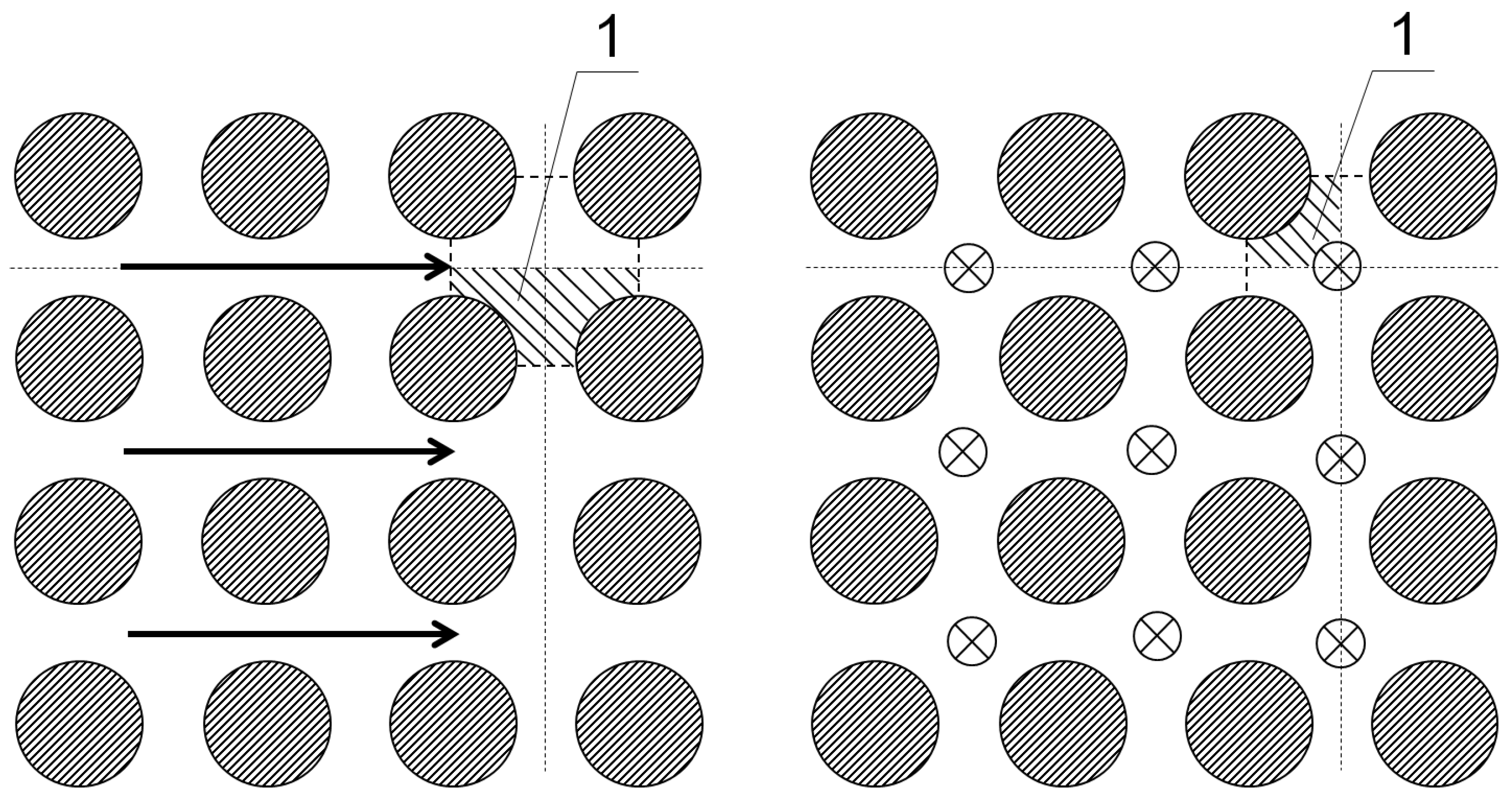
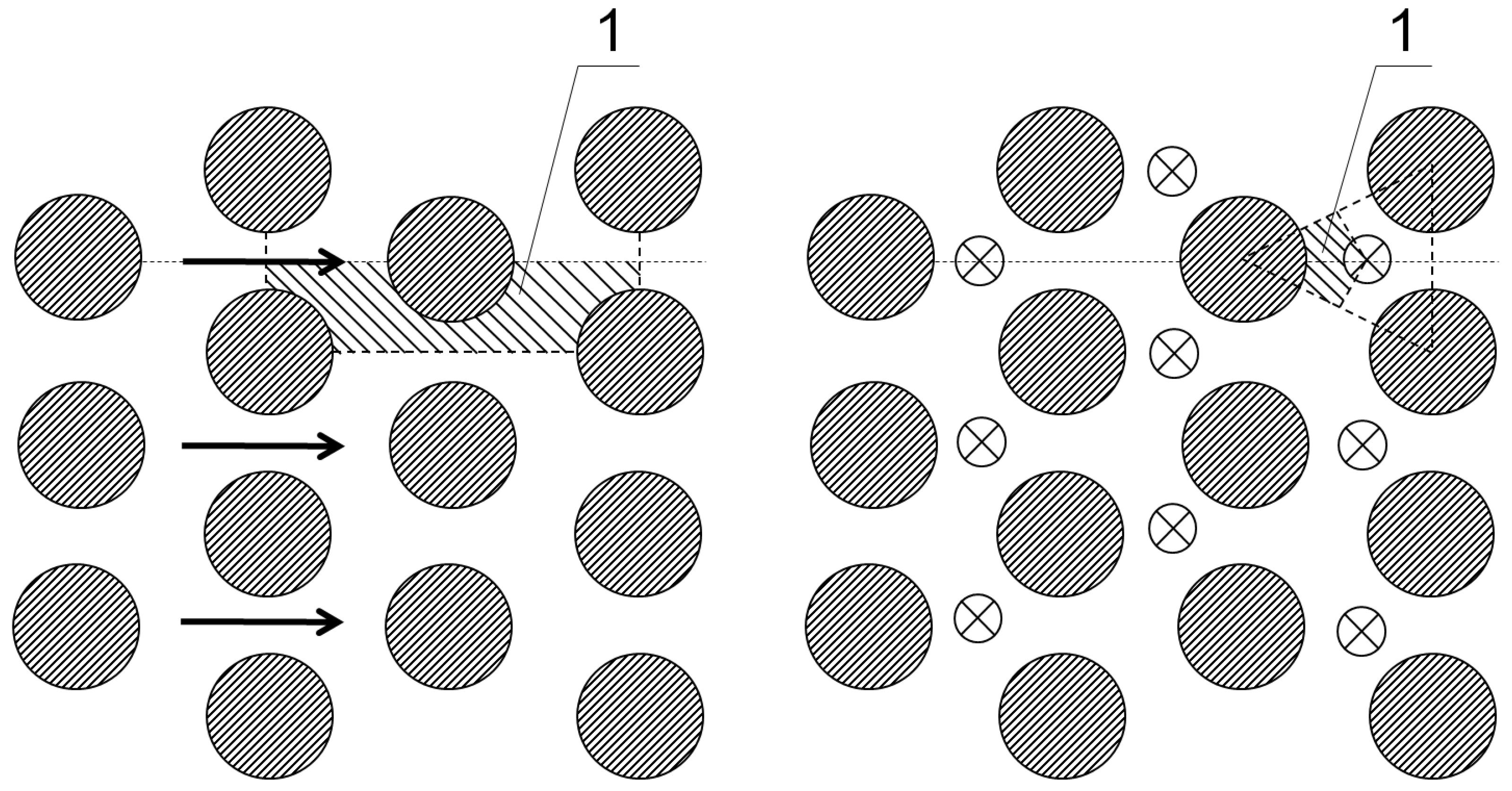
The transverse and longitudinal flow of water with a temperature of approximately 25 °C was simulated for the assembly of round rods (Figure 1 and Figure 2). The diameter of the rods was 10 mm. Reynolds number varied from 104 to 106. The ordinary definition of the Reynolds number in a bundle of rods was used. For a longitudinal flow, the Reynolds number was calculated by the average velocity in the cross-section of the rod bundle. In this case, the hydraulic diameter of an elementary regular bundle cell was used as a characteristic size. The Reynolds number was calculated by the average velocity in the narrow bundle section and the rod diameter in the case of a transverse flow. The porosity value varied from 0.4 to 0.8 by changing the pitch value. The length of the simulated section in the case of longitudinal flow was 20 mm.
The calculations were carried out using the standard local k−ε turbulence model [24] in the ANSYS CFX code [10]. The scalable wall functions were used in the calculation [10]. The scheme of the second order of accuracy for the convective term in the equations of the law of conservation of momentum and the second order of accuracy for the convective term in the equation of turbulent characteristics were used. Unbalance values less than 1% and maximum local residuals not more than 10−5 were chosen as criteria of convergence.
Periodic boundary conditions were set at the end boundaries of the computational domain with the specified flow rate. The boundary symmetry condition was set on the lateral surfaces. A no-slip condition was set on the wall.
The computational mesh was created using the ANSYS MESH program [25,26]. The size of the grid element was set in such a way as to obtain the grid convergence of the solution for the required integral parameters , , . Additionally, the pressure drop on the simulated domain was controlled. This drop was used to check simulation results by comparing it with the calculation based on empirical dependences from the reference book [27]. The resulting deviations of the pressure drop from those calculated from the experimental dependences did not exceed 10% for longitudinal flow and 20% for transverse flow, which are within the error of empirical dependences.
For the case of longitudinal flow, the number of mesh elements ranged from 353,880 to 788,000 for a triangular bundle of rods and from 528,560 to 1,163,640 for a square bundle of rods, depending on the Re number and porosity. In the direction of the fluid flow, the region was divided into 40 elements, with decreasing the mesh element size towards the boundaries (inlet and outlet). The y+ value varied in the range from 1 to 180.
For the case of transverse flow, the number of mesh elements ranged from 240,856 to 492,689 for a triangular bundle of rods and from 101,357 to 630,687 for a square bundle of rods, depending on the Re number and porosity. The y+ value varied in the range from 0.3 to 150.
The stationary distribution of velocities, pressure, kinetic energy of turbulence, and the rate of dissipation of kinetic energy of turbulence within the calculated volume were obtained. The integral characteristics of the flow were then obtained for cell-averaged values of the kinetic energy of turbulence k, the rate of dissipation of kinetic energy of turbulence ε, the coefficient of kinematic turbulent viscosity , and integral coefficient in expression (15).
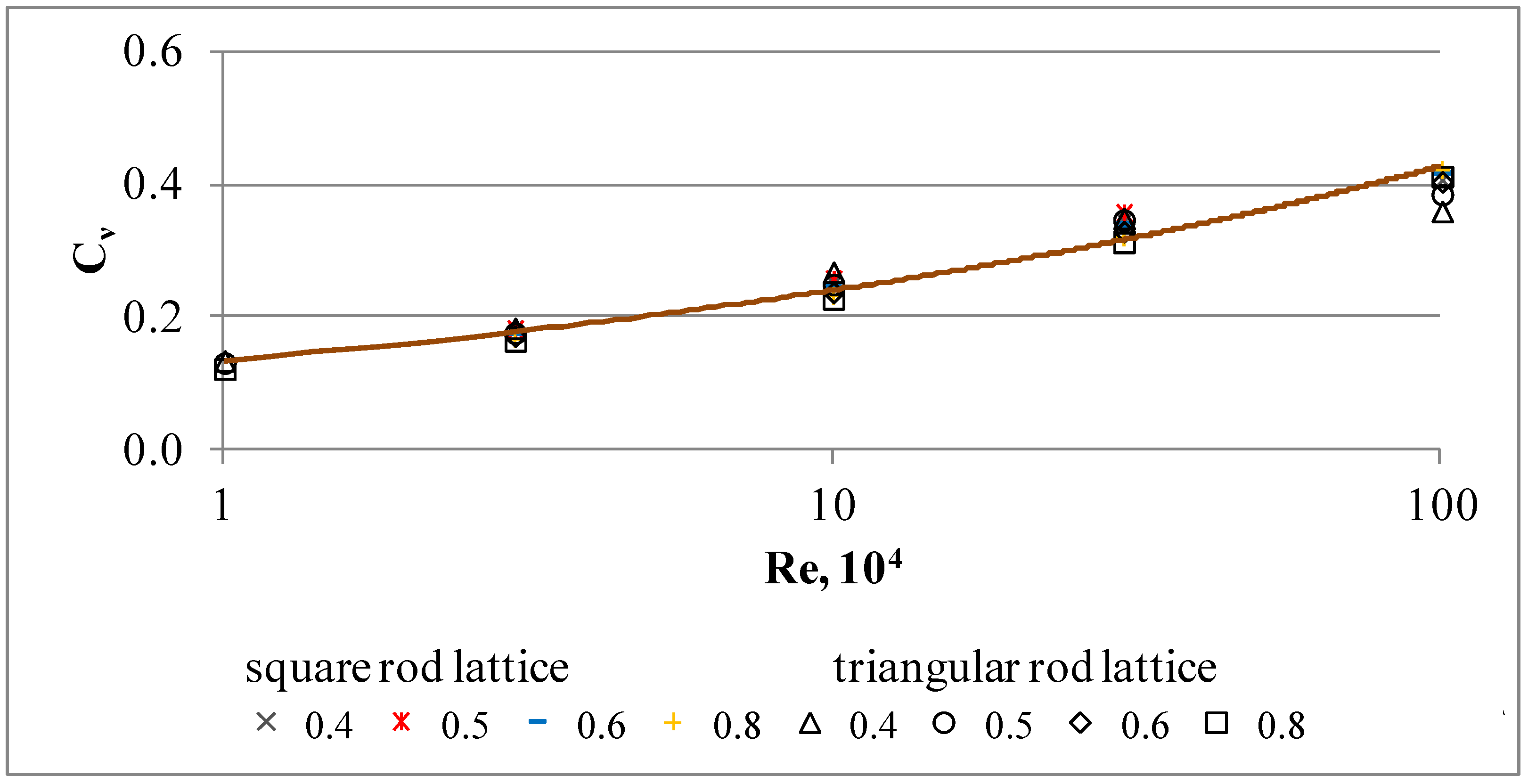
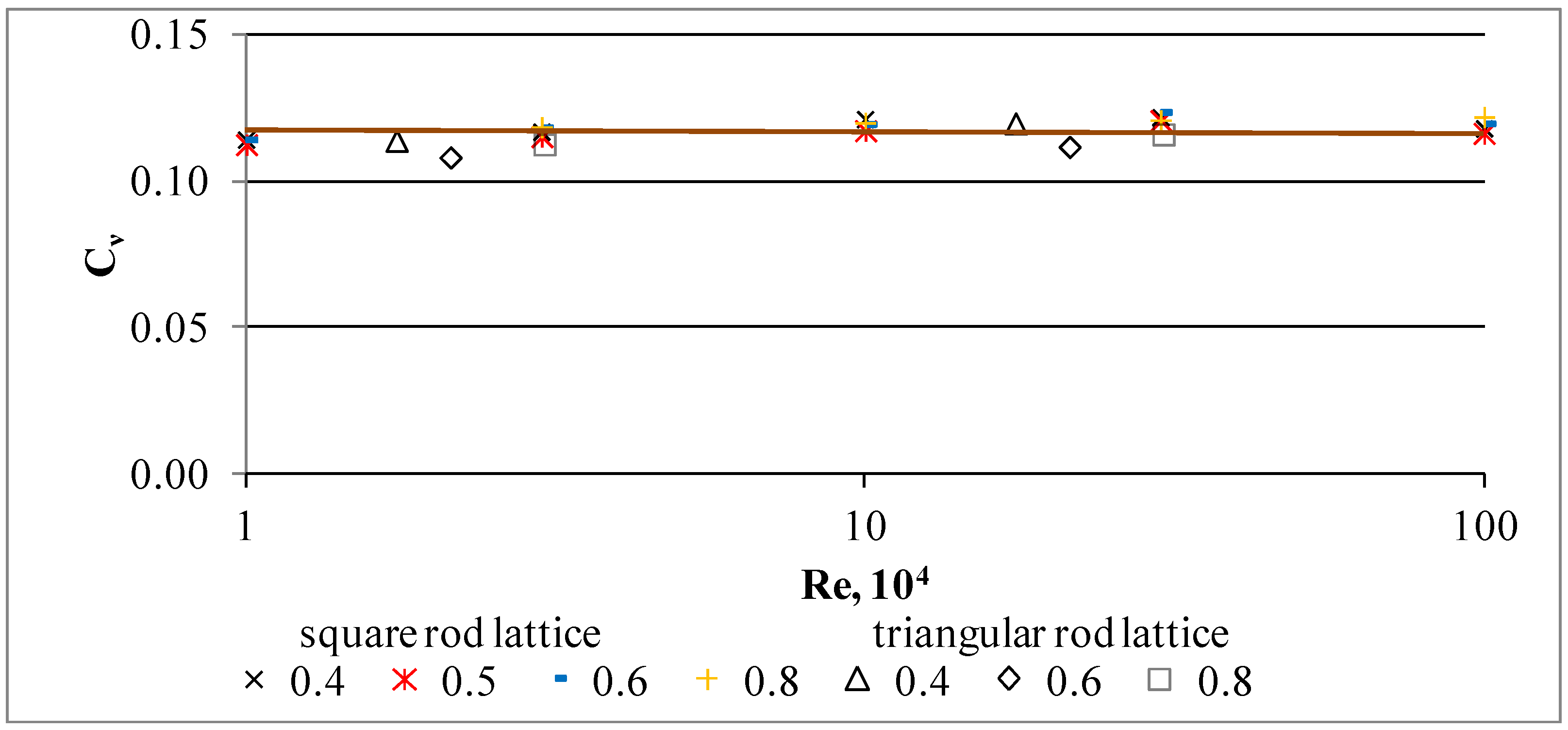
The dependences of the integral coefficient on the Re number for longitudinal and transverse flow around the assembly of round rods are shown in Figure 3 and Figure 4.
The integral coefficient is a function of the Reynolds number for longitudinal flow around the assembly of round rods:
In Equation (28), Re is the Reynolds number.
The integral coefficient is practically constant for a transverse flow around the assembly of round rods and can be taken equal to 0.117.
The dependence of the integral coefficient on the Re number for an arbitrary angle of flow around the assembly, in the first approximation, can be represented as follows:
In the local k−ε turbulence model, the coefficient is constant and equals 0.09 [28]. In the integral turbulence model, this coefficient is not a constant and depends both on the flow direction and on the Reynolds number but does not depend on the porosity of the structure or the type of rod assembly.
Figure 5 shows the dependence of the integral coefficient , on the Re number and the porosity of the assembly, which was calculated using Equation (27).
The figure shows that the integral coefficient increases from 0.2 to 0.7 with an increase in the Re number when it changes in the range from 104 to 106. It should be noted that the porosity of the structure and the type of packing of the rods have little effect on the value of . The results can be approximated by the following relationship:
The set of closing relations for smooth bundles of rods is determined by Equation (29) for the integral coefficient and Equation (30) for the integral coefficient .
4.2. Computational Studies of the Flow around Fuel Assemblies with a Spacer Grid and Wire-Wrapped Fuel Bundles
In fuel assemblies, fuel rod spacing is carried out using special spacer elements, which are spacer grids or wire winding on fuel rods. The spacer elements affect the flow of the coolant in the fuel assembly and require a corresponding correction of the integral turbulence model.
4.2.1. The Set of Closing Relations for Fuel Assemblies with a Spacer Grid
The presence of the spacer grid leads to a change in the form of the resistance tensor and the generation of turbulence in the spacer grid. The set of closing relations outside of the spacer grid area is the same as the set of closing relations for smooth bundles of rods (Equations (29) and (30)).
In the area of the spacer grid, the values of the tensor of resistance and the generation of turbulence change. The coefficient of hydraulic resistance for the spacer grid can be calculated using the following formula [29]:
In Equation (31), is the constraint coefficient and equals the ratio of the cross-sectional area to the area of the flow area of the channel; is the narrowing coefficient; lp is the height of the spacer grid; and Δ is the roughness of the spacer grid.
The rate of turbulent production due to deflection velocities can be calculated using the following formula:
In Equation (32), is the total turbulence energy generated by the spacer grid; is not equal to zero only in the spacer grid region; is the longitudinal coefficient of hydraulic resistance for a spacer grid; is the inlet flow velocity in the spacer grid region; and lp is the height of the spacer grid. The value of the integral coefficient must be determined for a spacer grid with the help of CFD modeling.
4.2.2. The Set of Closing Relations for Wire-Wrapped Fuel Bundles
In the area of the wire-wrapped fuel bundles, the values of the tensor of resistance change. The coefficients of hydraulic resistance for the wire-wrapped fuel bundles can be calculated using the following formulas [30,31] for longitudinal and transverse flow:
In Equations (33) and (34), is the coefficient of longitudinal hydraulic resistance for smooth rods; T is the wire lead length; d is the rod diameter; and s is the rod pitch.
It was shown earlier [32] that to describe the integral coefficients and one can use the dependence for smooth bundles of rods for wire-wrapped fuel bundles.
5. Numerical Implementation and Testing of the Developed Model
For the numerical solution of the equations of the porous body model and the integral turbulence model, FEM is used. The FEM is implemented using the DOLFIN library of the FEniCS package [33].
5.1. Variational Formulation of the Problem
The so-called weak form of the boundary value problem for the equations of the porous body model (1)–(3) together with the integral turbulence model (13)–(15) was obtained by multiplying the original differential equations by test functions and then using integration by parts [9] (to simplify the notation, the averaging signs were omitted):
In Equations (35)–(38), are test functions; is the area; is the area boundary; n is the normal to the surface; is the turbulent viscosity.
Equation (35) is written for the case of using a “coupled” approach to solving the equation of the law of conservation of momentum, which solves all equations for all desired variables for a particular element and repeats this process for all elements into which the computational domain is divided.
Taylor–Hood finite elements P2-P1 were used to discretize the equation of the law of conservation of momentum [34]. Lagrange finite elements were used for the equations of transfer of the kinetic energy of turbulence (36), the rate of dissipation of the kinetic energy of turbulence (37), and energy (38).
5.2. Scheme for Solving a System of Equations
At each time step, a nonstationary problem is solved with a given number of iterations. At each internal iteration, the equations for the velocity and pressure are first solved. The equations for the turbulence parameters are then solved. Next, the equations for the conservation of energy are solved. The solution of the equations occurs until the specified maximum number of iterations for the corresponding equation is exceeded, or upon reaching the specified calculation accuracy, depending on which comes first. Additionally, the imbalance value is calculated for the equation of the law of conservation of momentum. At the end of the iterative process, the results are saved in data file format provides by open-source, freely available Visualization Toolkit (VTK) [35].
5.3. Numerical Model Testing on a 19-Bar Experimental Assembly
Simulation of the experiment was performed. The experiment was previously carried out at the Institute for Physics and Power Engineering (IPPE) on an experimental 19-bar assembly [36]. In the experiment, Na−K was used as a coolant. The hexagonal fuel assembly used in the experiment consisted of 19 unheated smooth rods embedded in a hexagonal channel. The rod diameter was 19 mm and its relative pitch was 1.17. The apothem of the hexagonal channel was 49.4 mm. The rods were spaced by the upper and lower gratings [36]. The distance between gratings was 745 mm. The lower ends of the rods were fixed in the spacer grid. The upper ends of the rods were extended beyond the working length of the model and sealed in the flange [36]. Blocking of the flow area was carried out using a plate. The plate was installed in the central part of the fuel assembly cross-section at a distance of 380 mm from the lower grate and overlapped the cross-section of the assembly to the middle of the peripheral rows of rods, forming a 55% central blockade of the flow area. The blockade thickness was 8 mm. The longitudinal velocity was measured along the length by the electromagnetic method. In the experiment, the values of the emf of the electromagnetic sensor were obtained for the central, intermediate, lateral, and angular channels (see Figure 6).
Stationary isothermal coolant flow around the assembly was simulated. The physical properties of the Na-K coolant were calculated at a temperature of 100 °C. The Re number was 3.3 × 10⁴. The calculation was carried out until the stationary distribution of all the required parameters was obtained. The time step value varied in the range 10−3–10−4 depending on the magnitude of the current imbalances for the equation of the law of conservation of momentum.
At the input, a boundary condition of the first type was set for the velocity, energy, kinetic energy of turbulence, and its dissipation rate. The values for the kinetic energy of turbulence and its dissipation rate were calculated through the value of the turbulence intensity, which was set to 5%. At the output, a boundary condition of the first type was set for the pressure and a zero gradient for all other parameters. The outlet pressure was set equal to 1 atm. The slip boundary condition for the velocity and zero gradients for all other parameters were set on the wall.
The construction of the geometry and mesh of the computational domain was carried out in the GMSH program [37]. The geometry of the computational domain is a hexagonal prism with a height of 745 and a wrench size of 98.8 mm. Mesh elements are tetrahedrons. The mesh consists of 6795 nodes and 37,224 elements. The mesh was divided into several sub-areas to set the sizes of mesh elements more accurately in the blockade area and behind it. The blocking area was simulated by high hydraulic resistance.
As a result of the calculation, the stationary distribution of velocities, pressure, kinematic turbulent viscosity, kinetic energy of turbulence, and dissipation rate of kinetic energy of turbulence were measured. The analysis of the results was carried out using the ParaView program [38].
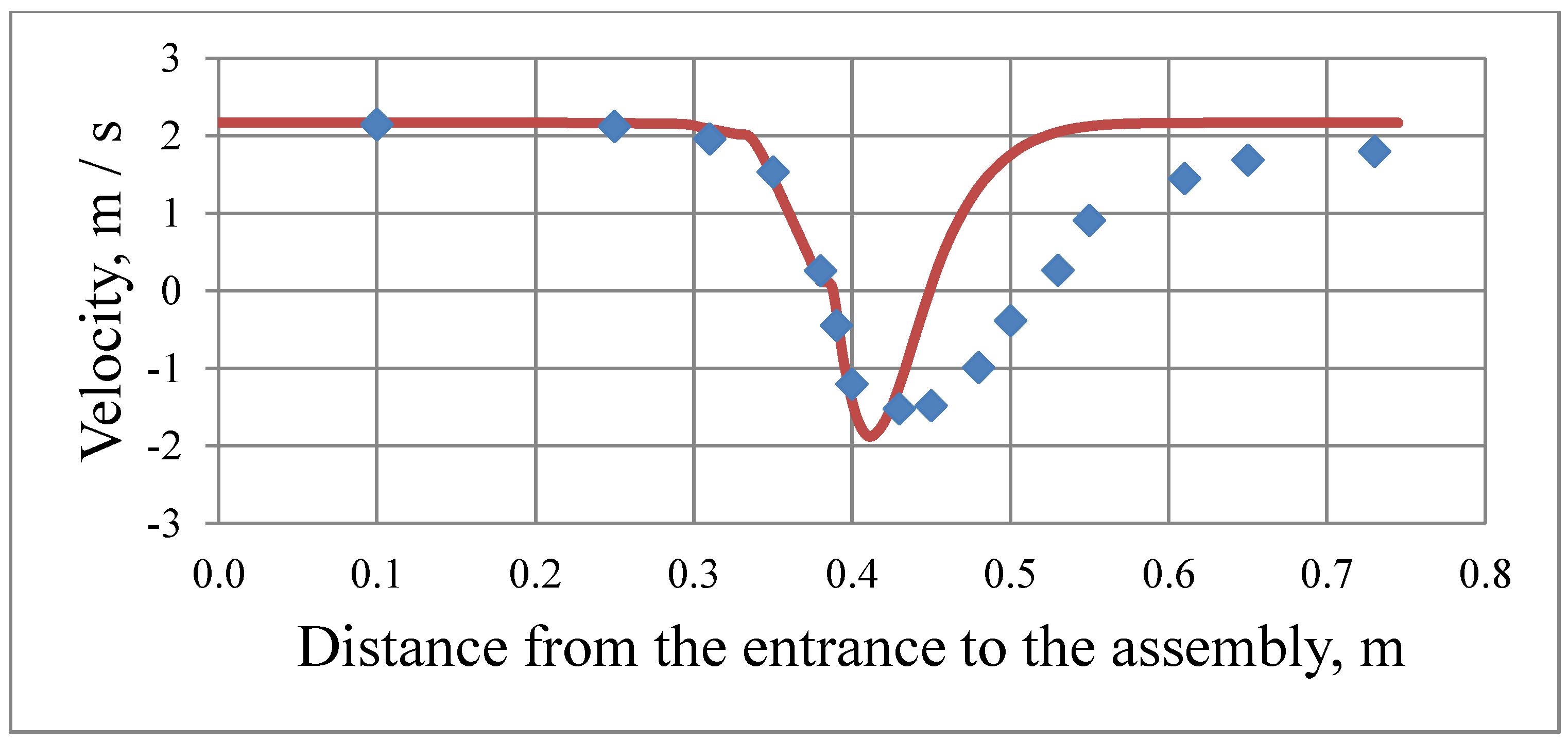
Figure 7 shows a comparison of the results of calculating the longitudinal velocity along with the height with experimental data for the central element. Because for the central element there is no unevenness of the velocity along its perimeter, the authors of [36] give as experimental data the values of the longitudinal velocity averaged over all points 1–7 in Figure 8. The calculated values on the axis passing through the geometric center of the model are used as the simulation results.
When comparing the results of calculating the longitudinal velocity along the height with the experimental data for the intermediate element, the presence of uneven velocity along the perimeter was considered. The values at the points shown in Figure 8 were taken as the calculation results.
Figure 9 shows a comparison of the results of calculations of the longitudinal velocity along with the height with the experimental data at point 3 for the element.
The simulation results qualitatively agree with the experimental results. Behind the blockade, there is a vortex region with a reverse flow (Figure 7 and Figure 9). The maximum reverse flow velocity is on the bundle axis. The vortex region size is determined by the distance from the blockade to the rear stagnation point with zero velocity. Downstream of this region, the flow velocity gradually returns to the inlet velocity.
The calculated velocity values in the section before the blockade are in good agreement with the experimental data. The error in determining the maximum reverse flow velocity lies within 10–15%. At the same time, the calculated size of the vortex region differs from the experimental one by more than 40%. In addition, the calculated flow velocity returns to the initial value faster.
One of the reasons for the decrease in the vortex region size can be the blocking model used. The experimental blockade was made by a special plate, so it was completely impenetrable. In the porous body model used in the calculation, the blockade is simulated by setting a high hydraulic resistance in the blocking area, and thus it is partially permeable. The blockade permeability is approximately 3–5%. The presence of a leak flow reduces the size of the recirculation area. At 55% central blockage, a leakage flow of approximately 30% eliminates the reverse flow region [39].
The faster return of the calculated flow velocity to the initial state is possibly related to the boundary conditions at the outlet of the computational domain. In the experiment, a grating was located at the outlet of the bundle. It undoubtedly interfered with the transverse velocity equalization. The grating was not considered in the calculation and the boundary condition of constant pressure was used.
A detailed analysis of the reasons for the obtained discrepancies will be performed in further studies.
6. Conclusions
A method for calculating the closing relations of a porous body model using an integral turbulence model has been developed. During computational studies, the parameters of the integral turbulence model and the closing relations of the porous body model for assemblies of smooth rods were determined. The integral coefficient is practically constant for a transverse flow around the assembly of round rods and can be taken equal to 0.117. The integral coefficient is a function of the Reynolds number for longitudinal flow around the assembly of round rods. The integral coefficient increases from 0.2 to 0.7 with increasing Reynolds from 104 to 106 and weakly depends on the porosity of the structure and the type of packing of the rods. The presence of the spacer grid leads to a change in the form of the resistance tensor and the generation of turbulence in the spacer grid. The value of the integral coefficient must be determined for a spacer grid with the help of CFD modeling. The presence of wire-wrapped fuel bundles leads to a change in the form of the resistance tensor. The integral coefficients and or wire-wrapped fuel bundles can be determined from the dependencies for smooth bundles of rods. The experiment simulation performed using the porous body model with the integral turbulence model confirmed the possibility of using this approach to describe thermal-hydraulic processes during fluid flow in rod structures. The scatter of the calculated values of coefficients and may be attributed to the dependence of this coefficient not only on the Reynolds number, but also on the initial fluctuations in the flow and near the wall. Therefore, improving the model is possible, considering the stochastic relations according to [40,41,42,43,44,45,46].
Author Contributions
Conceptualization, I.G.M.; methodology, I.G.M.; software, M.N.V.; validation, I.G.M. and M.N.V.; formal analysis, I.G.M. and M.N.V.; investigation, I.G.M. and M.N.V.; resources, I.G.M. and M.N.V.; data curation, I.G.M. and M.N.V.; writing—original draft preparation, M.N.V.; writing—review and editing, I.G.M. and M.N.V.; visualization, M.N.V.; supervision, I.G.M.; project administration, I.G.M.; funding acquisition, I.G.M. All authors have read and agreed to the published version of the manuscript.
Funding
This research received no external funding.
Data Availability Statement
The data present in this study are available on request from the corresponding author.
Acknowledgments
The authors express their sincere gratitude to A.S. Korsun for his help in choosing the direction of research and a useful discussion of its results.
Conflicts of Interest
The authors declare no conflict of interest.
References
- Rowe, D.S. Cross-Flow mixing between parallel flow channels during boiling Part-I COBRA-Computer program for coolant boiling in rod arrays. Nucl. Eng. Des. 2018, 332, 329–344. [Google Scholar]
- Rowe, D.S.; Angle, C.W. Cross Flow Mixing between Parallel Flow Channels during Boiling. Part II: Measurement of Flow and Enthalpy in Two Parallel Channels; Technical Report No. BNWL-371-Pt-2; Pacific Northwest Laboratory: Richland, DC, USA, 1967.
- Zhang, H.; Zou, L.; Zhao, H.; Martineau, R. Developing Fully Coupled Subchannel Model in RELAP-7; Idaho National Laboratory: Idaho Falls, ID, USA, 2014.
- Moorthia, A.; Sharmab, A.K.; Velusamyb, K. A review of sub-channel thermal-hydraulic codes for nuclear reactor core and future directions. Nucl. Eng. Des. 2018, 332, 329–344. [Google Scholar] [CrossRef]
- Liu, X.J.; Scarpelli, N. Development of a sub-channel code for liquid metal cooled fuel assembly. Ann. Nucl. Energy 2015, 77, 425–435. [Google Scholar] [CrossRef] [Green Version]
- Imke, U.; Sanchez, V.H. Validation of the Subchannel Code SUBCHANFLOW Using the NUPEC PWR Tests (PSBT). Sci. Technol. Nucl. Install. 2012, 2012, 465059. [Google Scholar] [CrossRef]
- Pedras, M.H.J.; de Lemos, M.J.S. Macroscopic turbulence modeling for incompressible flow through undeformable porous media. Int. J. Heat Mass Transfer 2001, 44, 1081–1093. [Google Scholar] [CrossRef]
- Korsun, A.S.; Kruglov, V.B.; Merinov, I.G.; Fedoseev, V.N.; Kharitonov, V.S. Heat and mass transfer when flowing around structures such as bundles of rods in the approximation of a porous body model. VANT Ser. Nucl. React. Const. 2014, 2, 88–95. Available online: https://vant.ippe.ru/year2014/2/842-9.html (accessed on 29 November 2021).
- Logg, A.; Kent-Andre, M.; Wells, G. The FEniCS Book. Automated Solution of Differential Equations by the Finite Element Method; Springer: Berlin, Germany, 2012; p. 732. Available online: https://fenicsproject.org/book/ (accessed on 29 November 2021).
- ANSYS, Inc. ANSYS CFX Help File; ANSYS, Inc.: Canonsburg, PA, USA, 2018. [Google Scholar]
- Wilcox, D.C. Turbulence Modeling for CFD, 3rd ed.; Birmingham Press: San Diego, CA, USA, 2006; p. 536. ISBN 978-1928729082. [Google Scholar]
- Garbaruk, A.V.; Strelets, M.h.; Travin, A.K.; Shur, M.L. Modern Approaches to Turbulence Modeling; Publishing House of the Polytechnic University: St. Petersburg, Russia, 2016. [Google Scholar]
- Roelofs, F.; Gopala, V.R.; Chandra, L.; Viellieber, M.; Class, A. Simulating fuel assemblies with low-resolution CFD approaches. Nucl. Eng. Des. 2012, 250, 548–559. [Google Scholar] [CrossRef]
- Smith, B.L. Assessment of CFD codes used in nuclear reactor safety simulations. Nucl. Eng. Technol. 2010, 42, 339–364. [Google Scholar] [CrossRef] [Green Version]
- Korsun, A.S.; Kruglov, A.B.; Kruglov, V.B.; Odintsov, A.A.; Kharitonov, V.S. Experimental study of resistance for angular flow around beams of rods. In Proceedings of the Thermophysics-2008, Obninsk, Russia, 15–17 October 2008. [Google Scholar]
- Horn, R.A.; Johnson, C.R. Matrix Analysis, 2nd ed.; Cambridge University Press: Cambridge, UK, 2012; p. 662. Available online: www.cambridge.org/9780521548236 (accessed on 29 November 2021).
- Vlasov, M.N.; Korsun, A.S.; Maslov, Y.A.; Merinov, I.G.; Kharitonov, V.S. Modeling of thermohydraulic processes in the cores of fast reactors. In Proceedings of the Thermophysics-2012, Obninsk, Russia, 24–26 October 2012. [Google Scholar]
- Vlasov, M.N.; Korsun, A.S.; Maslov, Y.A.; Merinov, I.G.; Rachkov, V.I.; Kharitonov, V.S. Determination of integral turbulence model parameters as applied to the calculation of rod-bundle flows in porous-body approximation. Thermophys. Aeromech. 2016, 23, 201–209. [Google Scholar] [CrossRef]
- Lemos, M.J.S. Turbulence in Porous Media: Modeling and Applications; Elsevier: Amsterdam, The Netherlands, 2006; p. 384. [Google Scholar] [CrossRef]
- Hinze, J.O. Turbulence, 2nd ed.; McGraw-Hill: New York, NY, USA, 1975; ISBN 978-0070290372. [Google Scholar]
- Tennekes, H.; Lumley, J.L. A First Course in Turbulence; MIT Press: Cambridge, MA, USA, 1972; ISBN 0262200198. [Google Scholar]
- Pedras, M.H.J.; de Lemos, M.J.S. Simulation of turbulent flow in porous media using a spatially periodic array and a low Re two-equation closure. Numer. Heat Transf. Part A Appl. 2001, 39, 35–59. [Google Scholar] [CrossRef]
- Pedras, M.H.J.; de Lemos, M.J.S. Computation of Turbulent Flow in Porous Media Using a Low-Reynolds Model and an Infinite Array of Transversally Displaced Elliptic Rods. Numer. Heat Transf. Part A Appl. 2003, 43, 585–602. [Google Scholar] [CrossRef]
- Launder, B.; Sharma, B.I. Application of the energy-dissipation model of turbulence to the calculation of flow near a spinning disc. Phys. Lett. Heat Mass Tranf. 1974, 1, 131–137. [Google Scholar] [CrossRef]
- ANSYS-Meshing. Available online: https://www.ansys.com/Products/Platform/ANSYS-Meshing (accessed on 29 November 2021).
- ANSYS Meshing User’s Guide; Release 15.0; ANSYS, Inc.: Canonsburg, PA, USA, 2013.
- Kirillov, P.L.; Bobkov, V.P.; Zhukov, A.V.; Yuriev, Y.S. Handbook of thermo-hydraulic calculations in nuclear power. In Thermal-Hydraulic Processes in Nuclear Power Plants; IzdAT: Moscow, Russia, 2010; Volume 1. [Google Scholar]
- CFD-Online. Available online: https://www.cfd-online.com/Wiki/Standard_k-epsilon_model (accessed on 29 November 2021).
- Kirillov, P.L.; Yuriev, Y.S. Hydrodynamic Calculations: Reference Tutorial; IPPE: Obninsk, Russia, 2007. [Google Scholar]
- Subbotin, V.I.; Ibragimov, M.K.; Ushakov, P.A.; Bobkov, V.P.; Zhukov, A.V.; Yuriev Yu, S. Hydrodynamics and Heat Transfer in Nuclear Power Plants (Calculation Basis); Atomizdat: Moscow, Russia, 1975; pp. 123–124. [Google Scholar]
- Yuryev Yu, S.; Kolpakov, A.P.; Efanov, A.D. Development of a hydrodynamic and thermal model of a porous body and its application to the calculation of nuclear reactors of the BN type. VANT Ser. Phys. Techn. Nuc. React. 1984, 41, 79–85. [Google Scholar]
- Vlasov, M.N.; Korsun, A.S.; Maslov, Y.A.; Merinov, I.G.; Kharitonov, V.S. Determination of integral turbulence model parameters as applied to the calculation of flows in fuel assemblies of fast reactors in porous-body approximation. IOP Conf. Ser. J. Phys. Conf. Ser. 2020, 1689, 12068. [Google Scholar] [CrossRef]
- FEniCSx. Available online: https://fenicsproject.org/download/ (accessed on 29 November 2021).
- Femtable. Available online: https://femtable.org/ (accessed on 29 November 2021).
- VTK. Available online: https://www.vtk.org/ (accessed on 29 November 2021).
- Zhukov, A.V.; Matyukhin, N.M.; Rymkevich, K.S. Influence of Blocking the Flow Section of a Model Assembly of a Fuel-Element Cassette of a Fast Reactor on the Distribution of Coolant Velocities; Preprint FEI-1479; IPPE: Obninsk, Russia, 1983. [Google Scholar]
- Gmsh. Available online: http://gmsh.info/ (accessed on 29 November 2021).
- ParaView. Available online: http://www.paraview.org/ (accessed on 29 November 2021).
- Hubler, F.; Peppler, W. Summary and Implications of Out-of-Pile Investigations of Local Cooling Disturbances in LMFBR Subassembly Geometry Under Single-Phase and Boiling Conditions; KfK Rep. 3927; Kernforschungszentrum Karlsruhe GmbH: Karlsruhe, Germany, 1985. [Google Scholar]
- Dmitrenko, A.V. Determination of the coefficients of heat transfer and friction in supercritical-pressure nuclear reactors with account of the intensity and scale of flow turbulence on the basis of the theory of stochastic equations and equivalence of measures. J. Eng. Phys. Thermophys. 2017, 90, 1288–1294. [Google Scholar] [CrossRef]
- Dmitrenko, A.V. Results of investigations of non-isothermal turbulent flows based on stochastic equations of the continuum and equivalence of measures. IOP Conf. Ser. J. Phys. Conf. Ser. 2018, 1009, 012017. [Google Scholar] [CrossRef] [Green Version]
- Dmitrenko, A.V. Calculation of pressure pulsations for a turbulent heterogeneous medium. Dokl. Phys. 2007, 52, 384–387. [Google Scholar] [CrossRef]
- Newton, P.K. The fate of random initial vorticity distributions for two-dimensional Euler equations on a sphere. J. Fluid Mech. 2016, 786, 1–4. [Google Scholar] [CrossRef] [Green Version]
- Faranda, D.; Sato, Y.; Saint-Michel, B.; Wiertel, C.; Padilla, V.; Dubrulle, B.; Daviaud, F. Stochastic Chaos in a Turbulent Swirling Flow. Phys. Rev. Lett. 2017, 119, 14502. [Google Scholar] [CrossRef] [Green Version]
- Grimm, F.; Reichling, G.; Ewert, R.; Dierke, J.; Noll, B.; Aigner, M. Stochastic and Direct Combustion Noise Simulation of a Gas Turbine Model Combustor. Acta Acust. Unit. Acust. 2017, 103, 262–275. [Google Scholar] [CrossRef] [Green Version]
- Dmitrenko, A.V. An estimation of turbulent vector fields, spectral and correlation functions depending on initial turbulence based on stochastic equations. The Landau fractal equation. Int. J. Fluid Mech. Res. 2016, 43, 271–280. [Google Scholar] [CrossRef]
Figure 1.
Square rod lattice. Transverse (left) and longitudinal (right) flow; 1—calculation domain.
Figure 1.
Square rod lattice. Transverse (left) and longitudinal (right) flow; 1—calculation domain.

Figure 2.
Triangular rod lattice. Transverse (left) and longitudinal (right) flow; 1—calculation domain.
Figure 2.
Triangular rod lattice. Transverse (left) and longitudinal (right) flow; 1—calculation domain.

Figure 3.
The integral coefficient for longitudinal flow around the assembly of round rods versus the Re number and porosity .
Figure 3.
The integral coefficient for longitudinal flow around the assembly of round rods versus the Re number and porosity .

Figure 4.
The integral coefficient for transverse flow around the assembly of round rods versus the Re number and porosity .
Figure 4.
The integral coefficient for transverse flow around the assembly of round rods versus the Re number and porosity .

Figure 5.
The integral coefficient for longitudinal flow around the assembly of round rods versus the Re number and porosity .
Figure 5.
The integral coefficient for longitudinal flow around the assembly of round rods versus the Re number and porosity .

Figure 6.
Designations of the rods of the experimental assembly of the IPPE: c—central, i—intermediate, l—lateral, a—angular.
Figure 6.
Designations of the rods of the experimental assembly of the IPPE: c—central, i—intermediate, l—lateral, a—angular.

Figure 7.
The distribution of the longitudinal velocity of the coolant along with the height of the central element. Markers—experimental values [36], solid line—calculation results.
Figure 7.
The distribution of the longitudinal velocity of the coolant along with the height of the central element. Markers—experimental values [36], solid line—calculation results.

Figure 8.
Points (1–7) at which the calculation results were compared with experimental data for the intermediate element (i).
Figure 8.
Points (1–7) at which the calculation results were compared with experimental data for the intermediate element (i).

Figure 9.
The distribution of the longitudinal velocity of the coolant along with the height of the intermediate element at point 3. Markers—experimental values [36], solid line—calculation results.
Figure 9.
The distribution of the longitudinal velocity of the coolant along with the height of the intermediate element at point 3. Markers—experimental values [36], solid line—calculation results.

Publisher’s Note: MDPI stays neutral with regard to jurisdictional claims in published maps and institutional affiliations. |
© 2022 by the authors. Licensee MDPI, Basel, Switzerland. This article is an open access article distributed under the terms and conditions of the Creative Commons Attribution (CC BY) license (https://creativecommons.org/licenses/by/4.0/).
Share and Cite
MDPI and ACS Style
Vlasov, M.N.; Merinov, I.G. Application of an Integral Turbulence Model to Close the Model of an Anisotropic Porous Body as Applied to Rod Structures. Fluids 2022, 7, 77. https://0-doi-org.brum.beds.ac.uk/10.3390/fluids7020077
AMA Style
Vlasov MN, Merinov IG. Application of an Integral Turbulence Model to Close the Model of an Anisotropic Porous Body as Applied to Rod Structures. Fluids. 2022; 7(2):77. https://0-doi-org.brum.beds.ac.uk/10.3390/fluids7020077
Chicago/Turabian StyleVlasov, Maksim N., and Igor G. Merinov. 2022. "Application of an Integral Turbulence Model to Close the Model of an Anisotropic Porous Body as Applied to Rod Structures" Fluids 7, no. 2: 77. https://0-doi-org.brum.beds.ac.uk/10.3390/fluids7020077