
Comparison of Flow Behavior in Saccular Aneurysm Models Using Proper Orthogonal Decomposition


1
Department of Soils and Water Systems, University of Idaho, Moscow, ID 83844, USA
2
Department of Mechanical Engineering, University of Idaho, Moscow, ID 83844, USA
*
Author to whom correspondence should be addressed.
Fluids 2022, 7(4), 123; https://0-doi-org.brum.beds.ac.uk/10.3390/fluids7040123
Submission received: 17 February 2022
/
Revised: 16 March 2022
/
Accepted: 20 March 2022
/
Published: 23 March 2022
(This article belongs to the Special Issue Recent Advances in Computational Methods in Fluid Dynamics and Applications, Volume II)
Abstract
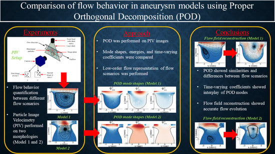
:Aneurysms are abnormal ballooning of a blood vessel. Previous studies have shown presence of complex flow structures in aneurysms. The objective of this study was to quantify the flow features observed in two selected saccular aneurysm geometries over a range of inflow conditions using Proper Orthogonal Decomposition (POD). For this purpose, two rigid-wall saccular aneurysm models geometries were used (i.e., the bottleneck factor of 1 and 1.6), and the inflow conditions were varied using a peak Reynolds number () from 50 and 270 and Womersley number () from 2 and 5. The velocity flow field data for the studied aneurysm geometries were acquired using Particle Image Velocimetry (PIV). The average flow field from the PIV measurement showed that the model geometry and have more significant impact on the average flow field than the variations in . The POD results showed that the method was able to quantify the flow field characteristics between the two model geometries. The mode shapes obtained showed different spatial structures for each inflow scenarios and models. The POD energy results showed that more than of the fluctuating kinetic energy were captured within five POD modes for flow scenarios, while they were captured within ten modes for . The time varying coefficient results showed the complex interplay of POD modes at different inflow scenarios, highlighting important modes at different phases of the flow cycle. The low-order reconstruction results showed that the vortical structure either proceeded outward or stayed within the aneurysm, and this behavior was highly dependent on , , and model geometry that were not evident in average PIV results.
1. Introduction
Aneurysms comprise the localized outpouching of a weakened blood vessel. Unruptured aneurysms constitute a growing public health concern [1] since individuals with unruptured aneurysms can be asymptomatic until the time of rupture [2]. A ruptured aneurysm can often cause subarachnoid hemorrhage (SAH), which has high mortality, long term disability rates, and high treatment costs [1,2]. Researchers from diverse backgrounds have worked on understanding aneurysm behavior and contributed significantly to the current understanding of aneurysm formation, growth, and rupture. Review articles from Brisman et al. [3], Lasheras [4], and Cebral and Raschi [5] have highlighted challenges in understanding aneurysm behavior due to its multi-disciplinary and multi-factorial characteristics.
One of the important parameters that play a role in aneurysm formation and progression is hemodynamics, and significant work has been conducted to understand its role in aneurysm pathophysiology [6,7,8,9,10,11,12,13,14]. Earlier studies have shown the presence of large-scale structures and patterns that are energetic in nature. These large-scale structures were observed to be a single vortical structure or multiple vortices in the aneurysm. The vortical structures remain stationary or become unstable and move throughout the cardiac cycle. In fusiform aneurysms, steady flow investigations by Budwig et al. [15] and Bluestein et al. [13] have shown that the flow field through an aneurysm is characterized by a recirculating vortex. Fukushima et al. [16] and Egelhoff [17] have shown that the vortices appear and disappear at different points in the cardiac cycle under pulsatile flow investigations. The trend of vortical structure behavior was also observed with other experimental and numerical studies [12,18,19,20,21,22]. Although the presence of these vortical structures has been studied extensively, understanding them better remains a challenge due to the complexity of flow patterns present inside the aneurysm sac that are dependent on incoming flow conditions [23,24].
Work has also been performed on the influence of inflow conditions and inflow waveforms on flow structure and behavior in the aneurysm. Le et al. [21] showed that the flow behavior can be cavity-flow driven or an unstable vortex ring formation driven based on flow pulsatility and aneurysm neck and diameter parameters. They defined a non-dimensional parameter to quantify aneurysm flow behavior, which had been used in other studies in saccular, bifurcation, and patient specific aneurysm models [25,26] and illustrated its robustness in quantifying aneurysm flow behavior. Asgharzadeh and Borazjani [27] found in their study that Reynolds number (Re) and Womersley number can be used to control the vortex structure locations. These studies have shown that inflow conditions impact flow behavior in an aneurysm, particularly in vortex formation and evolution processes.
Advancements in computational power have allowed researchers to utilize advanced data analysis methods to study and understand different fluid flows in great detail. One of these methods is Proper Orthogonal Decomposition (POD), which was initially introduced by Lumley [28] to extract coherent structures from turbulent flow fields. Since its introduction, POD has become a commonly used method for extracting coherent structures from experimental or computational data. POD optimally determines a basis of orthogonal functions, which span the data in the sense [29]. The most important property of POD is its optimality as it provides an efficient method of capturing the dominant components of a high-dimensional process using only a finite amount of modes [30]. Since its introduction, POD has been used in a variety of studies that are briefly introduced here [28,31,32,33,34,35]. Lumley [28] used POD to separate ’large eddies’ in shear flows. Graftieux et al. [31] suggested using POD to separate pseudo-fluctuations attributed to the unsteady nature of large-scale vortices from fluctuations due to small-scale turbulence. Chen et al. [32] used POD to quantitatively distinguish internal combustion engine flows with extreme flow properties. In biofluids, Byrne et al. [33] used POD in conjunction with computational fluid dynamics simulations to classify aneurysm hemodynamics according to spatial complexity and temporal stability for the parameters estimated from vortex core lines. They found that ruptured aneurysms have complex and unstable dynamics, while simple and stable dynamics are found in unruptured aneurysms. Daroczy et al. [34] used POD to determine spectral entropy in the flow, which helped them to appropriately select computational models based on flow regimes. Janiga [35] introduced POD for the analysis of time-varying three-dimensional hemodynamic data. His work showed the ability of POD to reduce the complexity of the time-dependent data for quantitative assessment. Yu et al. [23] used POD to study the impact of inflow conditions on flow behavior in an idealized experimental aneurysm. Their work highlighted that flow features were influenced by POD modes and the interplay of their POD coefficients.
A review of the previously mentioned studies indicates that aneurysms flows are a widely studied fluid dynamics problem. Advancements in experimental and computational capabilities have allowed researchers to parametrically study aneurysms in different models and flow conditions in greater detail than before. Computational aneurysm studies have enabled researchers to simulate different aneurysm flow scenarios and allowed them to model realistic aneurysm geometries using patient specific data [25,26,27,36,37,38,39,40,41,42,43,44]. However, the validation of numerical and computational studies still present some challenges, particularly in flow model and assumptions [45]. Experimental aneurysm studies also present some challenges, particularly the realistic fabrication of the model [46,47,48,49,50,51], optical access to the flow for flow field measurements [52,53,54] and measurement optimization approaches [55,56,57].
The presence of complex flow structures are still present in computational and experimental approaches and has encouraged the use of decomposition techniques to investigate flow physics in aneurysms. Recent work has shown the usefulness of POD in analyzing the spatial and temporal behavior in aneurysm flows. The approach of using POD can aid researchers in complex flow quantification as well as in comparisons with numerical and computational data. Despite the advantage of using POD, there are limited experimental fluid dynamics studies utilizing POD for analyzing complex flows in aneurysm. Therefore, the primary objective of this study is to quantify prominent flow features present in aneurysm flows for two selected geometries. For this investigation, inflow conditions were varied by changing non-dimensional parameters, namely Reynolds () number from 50 and 270 and Womersley () numbers from 2 and 5. POD was used to analyze coherent flow structures and to quantify their spatial characteristics. The flow field evolution inside the aneurysm test section was captured using Particle Image Velocimetry (PIV). The results showed that POD was able to accurately quantify the flow field characteristics for the two model geometries that were studied in this investigation. The POD modes illustrated similarities and dissimilarities of flow features at different inflow conditions and the POD time-varying coefficients provided a temporal interplay of POD modes and showed differences between flow cases. The flow field reconstruction using POD provided an accurate representation of the flow evolution highlighting the complex interplay of modes and their time-varying coefficients.
This investigation is organized as follows: First, a discussion on the experimental setup will be provided. This will be followed by an analysis approach and the Results and Discussion sections. Lastly, the summary and conclusions of findings for this study will be discussed.
2. Materials and Methods
This section provides details of the experimental setup and test conditions used for this study. First, a brief description of the aneurysm models will be provided. Details of the PIV setup and the pump used for this investigation will then be discussed. Lastly, information on the test conditions will be provided. Further details of the experimental setup, design, and flow quantification are provided by Yu et al. [23] and Yu and Durgesh [24].
2.1. Aneurysm Models and Fluid
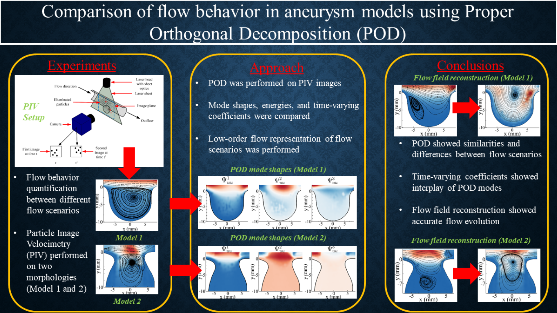
Experiments were performed on straight, rigid, idealized, sidewall aneurysm models; the schematics for the two models used in this investigation are shown in Figure 1a,b. The figures highlight the important features of the models, which have dimensions for , , , and . The aneurysm models are designed to have a long entry length in the cylindrical pipe () and allowed the fluid to fully develop prior to reaching the aneurysm region [58]. The return section () allowed flow disturbances to dissipate before recirculating back in the flow loop. The aneurysm geometries were spherical in shape, with maximum aneurysm sac diameters () and neck diameters () at mm for the model in Figure 1a and mm and mm for the model in Figure 1b. For this study, the aneurysm dimensions were characterized using bottleneck factor () [59] to provide a distinction between the models and their flow characteristics. The is the ratio of the maximum aneurysm diameter to the neck diameter opening, which provides for the model in Figure 1a and in Figure 1b.
The aneurysm models were fabricated at a professional glass shop. The borosilicate glass material was selected for the study as it is hydraulically smooth, and it allows accurate index matching with a commercially available fluid. The index of refraction matching enabled the flow structures in the aneurysm geometry to be optically accessed with minimal distortion. The aneurysm models were carefully inspected after fabrication. The neck edges were found to be smooth in the aneurysm geometries during their fabrication. Aneurysm model dimensions were also verified using a calibrated image plane. The inspection showed the pipe distance to the sac center (see Figure 1a,b) to be approximately 7 mm.
Aqueous glycerin was used in the current investigation to accurately match the index of refraction with the aneurysm models’ material. Aqueous glycerin was chosen as its fluid properties are known and has been previously used in other investigations [12,16,19,23,48,60]. The aqueous mixture of 60:40 by volume had a density of and a kinematic viscosity of . Non-dimensional parameters and [61] were used to characterize inflow conditions. The velocity scales and characteristic length scales were adjusted to match the flow regimes commonly found in the cerebral circulatory system [21,27,58,62,63].
2.2. Velocity Field Measurements
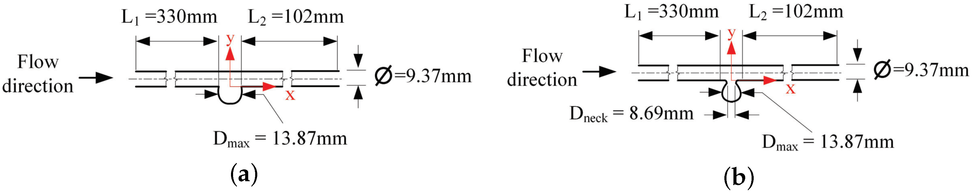
Velocity field measurements were performed on the aneurysm models using 2D PIV. Figure 2 shows a simplified schematic of the PIV system setup. The PIV system has a 200 mJ Nd:YAG double pulsed laser capable of pulsing at 15 Hz. The system also has a high resolution CCD camera (8 MP, 3312 × 2488 pixels) with a macro lens used to focus on the aneurysm region. The measurement plane was calibrated prior to experiments and had ≈0.012 mm/pixel spatial resolution. The calibration yielded a field of view of the aneurysm region to be 32 mm × 20 mm. A laser sheet thickness of 1 mm at the focal point was created using sheet optics.
The flow was seeded using silver-coated, neutrally buoyant, hollow glass spheres that were 9–13 μm in diameter. The aneurysm field of view was divided into three subregions, namely pipe, neck, and sac in order to appropriately select the time between PIV image pairs between the subregions. This approach made it possible to capture the flow structures at these subregions. To acquire an entire flow cycle, PIV images were acquired using a camera frame rate of Hz and sequenced to a single cycle. This method allowed us to capture different phases of the flow cycle, which were used for POD analyses. Velocity fields were determined from the PIV images using DaVis software. Post-processing used cross-correlation, multi-pass analyses with 50% overlap, and a final interrogation window of 32 × 32 pixels. The resulting velocity fields in the aneurysm yielded ≈9000, 6000, and 6800 velocity vectors in the pipe, neck, and sac regions, respectively.
2.3. Pump System
and were two inflow parameters used in this study, and these were controlled using a ViVitro Labs Inc. (Victoria, BC, Canada) SuperPump system. The piston pump system was used to move the fluid into the aneurysm model where the flow’s structure and behavior were captured by the PIV system. The pump system was capable of moving the piston at a frequency range of Hz to Hz. The system also featured a precise control of the flow rate and predefined waveform settings for the piston to follow. The design of the pump head contained spring-loaded disc valves that, in turn, allowed a uni-directional flow in the flow loop. The flow loop, thus, mimicked typical flows occurring in the human circulatory system.
In this study, piston stroke lengths of 2 mL to 50 mL and pump frequencies of Hz to Hz were used and correlated to non-dimensional fluid parameters and . The pump frequency of Hz corresponded to , while the pump frequency of Hz corresponded to flow conditions. A well-behaved sinusoidal waveform signal was selected for the piston to follow. The piston followed a periodic cycle with the other half of the waveform signal rectified due to the disc-valve’s design.
The flow fields were correlated to the flow cycle by synchronizing the PIV and pump systems. The synchronization of the hardware equipment was performed by simultaneously recording the PIV trigger signal and piston waveform during the experiments. The synchronization setup enabled us to determine when each PIV image was taken in relation to the flow cycle. The information acquired was then used for POD and flow evolution analyses.
2.4. Test Conditions
The inflow conditions for this study were varied by changing and [61]. These inflow parameters influence the flow’s structure and behavior in the aneurysm. Using the information from the pump and aneurysm model design, the pump piston frequency and pipe fluid velocity were then non-dimensionalized using and and provided as follows:
where is kinematic viscosity of the fluid, is diameter of the pipe, and f is flow frequency generated by the pump. The diameter of the pipe was used for the length scale (), while the maximum centerline velocity from the pipe () was used for the velocity scale. was then varied from 50 and 270, and varied from 2 and 5. The selected for this study represents quasi-steady flow and unsteady flow regimes, as identified by White [64]. Furthermore, the and conditions selected in this study were in the range of flow conditions used in previous studies [21,27,58,62,63]. For example, Steiger et al. [62] investigated basic flow structures in saccular aneurysms using a mean Reynolds number of 300 and an of 1.3 for pulsatile flow investigations. Work by Ku [58] had shown that the mean Reynolds number was around 300, and the Womersley number was about 4 in the carotid artery bifurcations located along the sides of the neck. Liou and Liou [63] used a mean Reynolds number of 500 to study human basilar tip aneurysms. Le et al. [21] used range of peak Reynolds number range from 375 to 800 and of 3.3–4.8. The computational studies by Asgharzadeh and Borazjani [27] in their computational study investigated the effect of mean Reynolds number and in intracranial aneurysms for a mean Reynolds number of 173–914 and of 5 to 30.
The test scenarios used and measurements performed for this investigation are summarized in Table 1. For each test scenario, dynamic equilibrium was achieved by waiting for several pump cycles. For scenarios, 170 complete pump cycles were acquired while 1040 complete pump cycles were obtained for . The table also shows the PIV frame rate chosen such that PIV images were acquired at a slightly different rate than the sub-multiples of the pump-driving frequency. The approach allowed PIV to capture different phases of the flow cycle [65]. The synchronization of the pump and PIV enabled velocity fields to be sequenced according to their phase in the flow cycle. This information was then used in the POD analyses, which helped in creating a flow evolution for a single flow cycle.
2.5. POD
POD was utilized to extract the energetic features or modes in the flow field. POD was used to understand flow behavior in the present study by isolating different flow features or modes and describing them through their energy content levels. Furthermore, the interplay of these modes along with their time-varying coefficients can provide a mathematical description of the flow field.
The mathematical background and description of POD are provided in great detail by several authors [28,30,66,67]. In the current investigation, a traditional (i.e.,vector POD) approach was used to ensure the coupling of u and v components of velocity.
POD is a method that aims to find a basis in the Hilbert space (i.e., ) that is optimal for the dataset and that can be represented in the following form:
where is a velocity field, and is the time-varying coefficient of the ith basis function () at time t. To find basis functions , they are chosen such that the averaged projection of the velocity field onto is maximized. This is shown as follows:
where denotes the modulus, is the ensemble average, represents the inner product, and denotes the norm. The solution to Equation (4) yields the approximation of the velocity field by a single function, but other critical points of this function are also physically significant. Thus, the set of functions, when taken together, provide the desired basis. This yields a variational calculus problem shown as follows.
A necessary condition is that the derivatives vanish for all variations , . In other words, we have the following.
Using calculus principles, the equation reduces to an Euler–Lagrangian equation shown as follows:
where is the domain of interest, is the spatial correlation of the velocity field, ⊗ is the tensor product, and is the energy associated with each POD mode. With further simplification and substitution, the formulation in Equation (7) can be described as follows:
where is the kernel of the POD formulation, i.e., the spatial velocity correlation matrix that results from the definition of velocity vector tensor product. The resulting simplification can be observed as an eigenvalue problem that is shown as follows:
where the eigen decomposition will have eigenvectors (i.e., POD modes) and , and represents the eigenvalues or energies captured by POD modes. The velocity field reconstruction in Equation (3) requires coefficients , which can be found by projecting the original velocity fields onto each of the POD modes and are provided as follows.
POD was implemented in-house using MATLAB. For each experimental inflow condition, 500 PIV images were acquired, which spanned several minutes. PIV images were acquired over 170 pump cycles for cases while 1040 complete pump cycles for cases. The average velocity flow field was subtracted for each inflow scenario before using POD, which allowed us to capture POD modes based on the flow fluctuations in the data set. POD implementation used a coupled u and v components of each velocity field, with auto and cross correlations operations to obtain the POD kernel (i.e., ). This coupling approach allowed the POD method to acquire the flow structures that were dependent on the u and v components of velocity, which were similar to the implementation used by Durgesh and Naughton [68]. For this study, the POD kernel was a square matrix of ∼13,000 × 13,000 elements. The mathematical formulation provided in Equation (9) was solved to calculate the eigenvalues (i.e., ) and eigenvectors (i.e., and ), where the subscript i represents POD mode numbers. The typical calculation processing time for POD analysis was approximately one hour. The obtained eigenvectors (i.e., POD modes) were then used to calculate the time-varying coefficients (i.e., Equation (10)) at a given time instance, and the low-order velocity field was performed using Equation (3).
3. Results
This section provides a discussion of the results obtained in this study. The average flow field results in the aneurysm region are presented to provide an overview of the flow features. The results from POD analysis are then presented, which include key results for POD modes, energies, and time-varying coefficients; and low-order reconstructions for both models. For brevity, only critical results in the aneurysm region are discussed here.
3.1. Average Flow Field
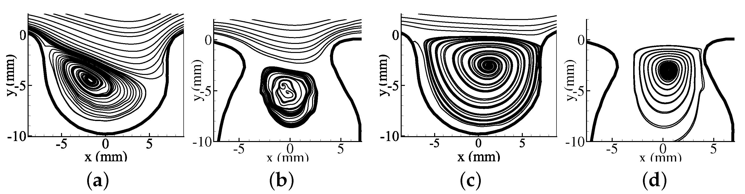
The mean flow results are first shown here to provide an overview of the bulk flow features at different inflow conditions. The time-averaged velocity fields for at different and are shown in Figure 3a–d. For each test scenario, 500 PIV images were used to calculate the time-averaged flow field. As seen from the figures, the mean flow results qualitatively indicate that the aneurysm is dominated by a clockwise vortex structure at different inflow conditions.
At and (i.e., Figure 3a), the vortex structure is pushed deep near the proximal side of the aneurysm sac with the average impinging location near the maximum aneurysm diameter (i.e., mm and mm). The closely compact streamlines near the distal neck (i.e., mm and mm) show high velocity gradients, which suggest an increase in shear stresses in this area. For (i.e., Figure 3b), the center of the vortical structure is below the neck diameter with the average impinging location near ( mm, mm). High velocity gradients are observed near the neck diameter (i.e., high shear stresses) as the incoming flow is diverted to the distal side for this . Similar average vortical structure shapes are observed for and scenarios, which are not discussed here.
For , there is a shift in flow behavior where the vortical structure (i.e., Figure 3c) engulfs the aneurysm sac for . The average impinging location moves closer to the distal neck (i.e., mm and mm) when compared to , while high shear stress is still observed in this area. With (i.e., Figure 3d), the vortex structure core moves near the neck diameter (i.e., mm, mm) with the average impinging locations and high velocity gradients near the neck area. Similar average vortical structure shapes are also observed for and scenarios, and they are not discussed here.
The average flow field results show that impacts the mean vortex structure shapes more than . When is compared across different and , the mean vortical shapes remain qualitatively similar. On the other hand, shows a engulfing vortical structure across different and . The impact of can be observed through the size of the vortical structure as the neck constricts this vortex. The similarity of the mean vortical shapes provides motivation to further investigate vortical structures and learn more about flow field behavior using POD.
3.2. POD Modes
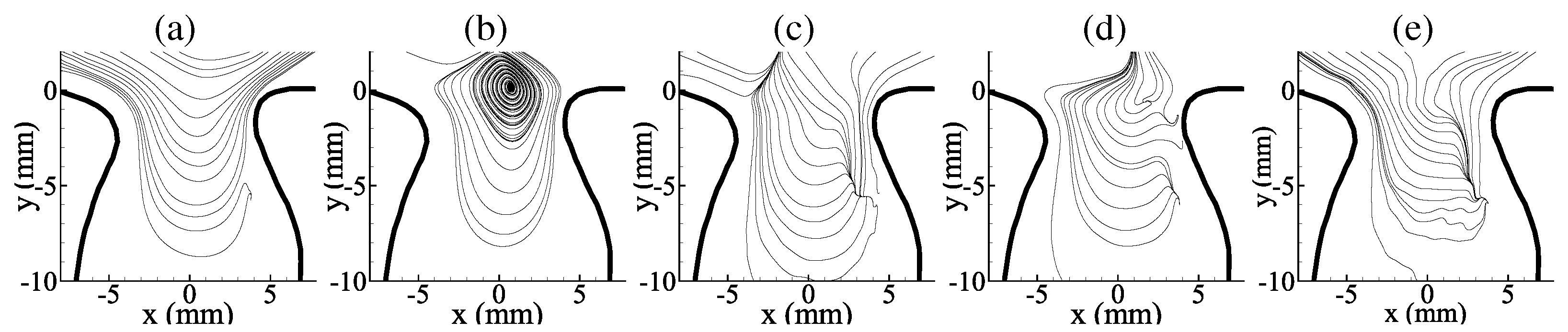
The POD mode results are presented here as they provide insights into large-scale flow structures and their underlying behavior. The POD modes shown here provide a mathematical description of the behavior of the flow structures present in the aneurysm, and they are ordered (i.e., the POD modes are ranked based on the fluctuating kinetic energies captured by them). The POD modes will have components and for streamwise and transverse components, respectively. For brevity, vector representation of the POD modes are presented and discussed in the manuscript.
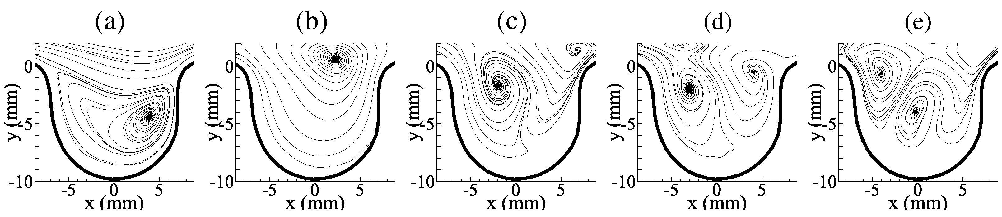
The first five POD modes () for , , and are shown in Figure 4a–e. The POD mode results for show different and distinct coherent structures within the aneurysm region. Such a variation in mode shapes allows for the convective motion of vortical structure. For a detailed discussion of the POD mode’s results for , see Yu et al. [23]. The POD mode results for , , and are shown in Figure 5a–e. Here, the overall POD modes are different from the ones observed in . POD modes still have symmetrical and asymmetrical features. Such features in the POD modes allow it to capture the convection of coherent structures. It should be noted that most of the spatial features in the POD modes are limited to the neck region of the aneurysm, suggesting that the coherent flow structure and its movements are confined to these locations for this model.
Next, the POD modes for the higher (i.e., 5) and for both models are analyzed. Figure 6a–e and Figure 7 show the POD modes for and , respectively. As observed in the figures, a change in results in very different sets of POD modes as compared to case for both s (see Figure 4 and Figure 5). This suggests that a change in impacts the flow features for both models. For model, we observe a variation in POD mode shapes inside the aneurysm sac, while for , most of the variations in the POD contour are confined to the neck region of the aneurysm sac. This suggests the presence of complex flow structures and their movement in the aneurysm sac for as compared to . It should also be noted that the POD mode shapes are significantly different for higher (i.e., 5) as compared to .
The POD mode shapes provide completely different spatial features between the two morphologies and inflow scenarios. The impact of is highlighted as the POD mode shapes show where distinct features and large-scale structures may be located. When inflow conditions are compared, the POD modes provide information on spatial features as well as the movement of large-scale structures. Next, we analyze the energy content of the POD modes to quantify the impact of POD modes on flow behavior.
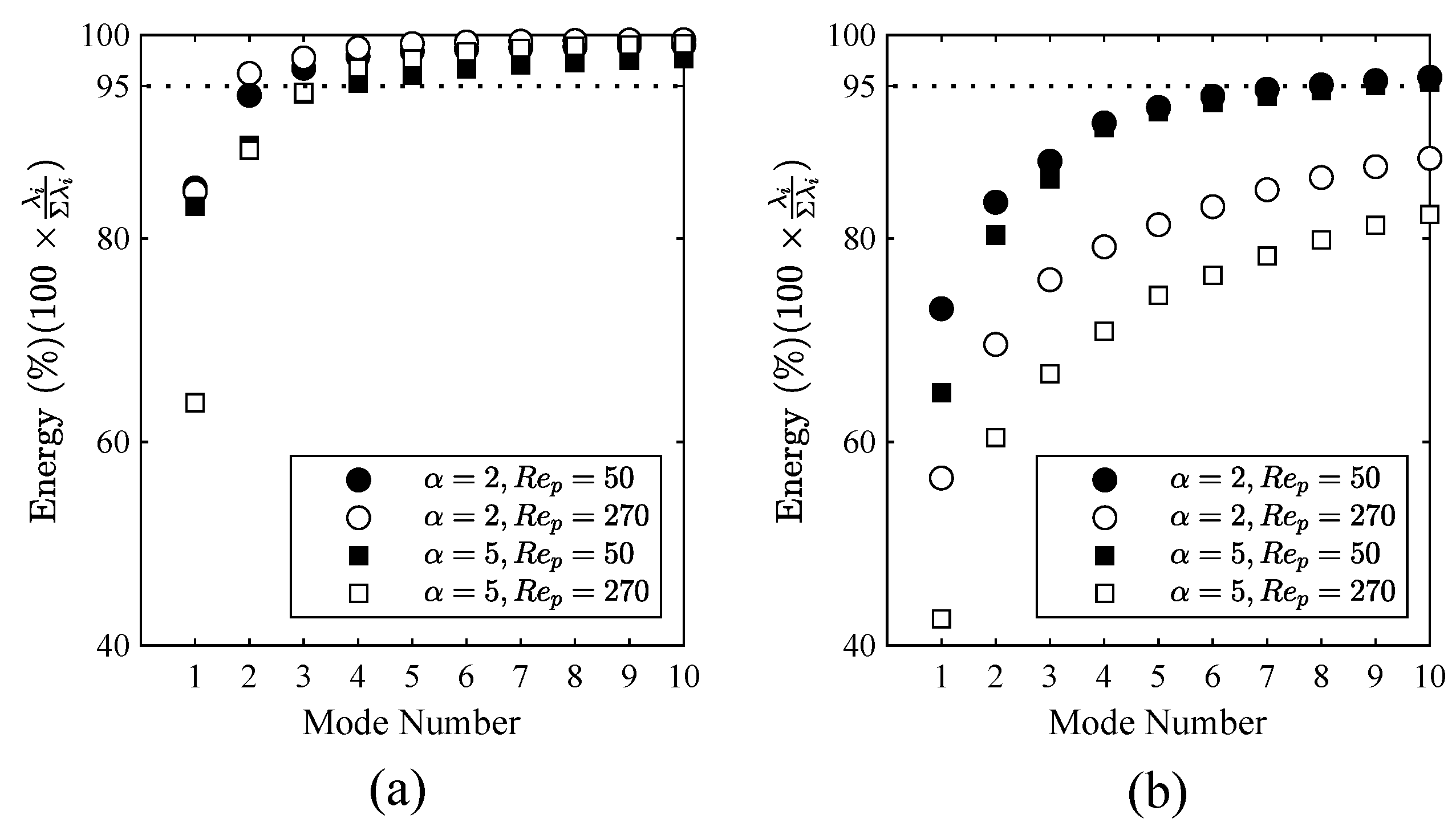
3.3. POD Energies
The relative POD energy (i.e., the ratio of energy captured by each POD mode and total fluctuating kinetic energy) results are analyzed to gain insight into the contribution of each POD mode. The results are shown in Figure 8 for the first ten modes for (Figure 8a) and (Figure 8b). As observed from these figures, the contribution of each POD mode decreases with increasing POD mode numbers. For (Figure 8a), the results indicate that about 95% of the fluctuating energy can be captured by five POD modes. For flow scenarios with , the first three mode shapes are likely to have dominating influences on the flow behavior in the aneurysm. This is in contrast with flow conditions, where five POD modes are needed to meet the threshold. Similar conclusions can be deduced for and scenarios (i.e., three modes) and scenarios (i.e., five POD modes).
In contrast to case, the energy results for exhibit different behaviors, as shown in Figure 8b. The results for this morphology show an increased number of modes required to reach a ∼95% of the total fluctuating kinetic energy. The scenarios show that at least five POD modes are needed to capture ∼95% of the total fluctuating kinetic energy. On the other hand, scenarios show that at least ten POD modes are needed to fully reconstruct an accurate representation of the flow field. Furthermore, the POD energy results for clearly show that impacts energy contributions.
The POD energy results suggest that aneurysm morphology and inflow conditions impact flow behavior. The energy results show critical differences between the two morphologies and provide an insight into the impact of inflow conditions on the large-scale structures in the aneurysm. To understand the dynamics of the POD modes and the interplay among the POD modes, the time-varying coefficients of the POD modes are analyzed.
3.4. POD Time-Varying Coefficients
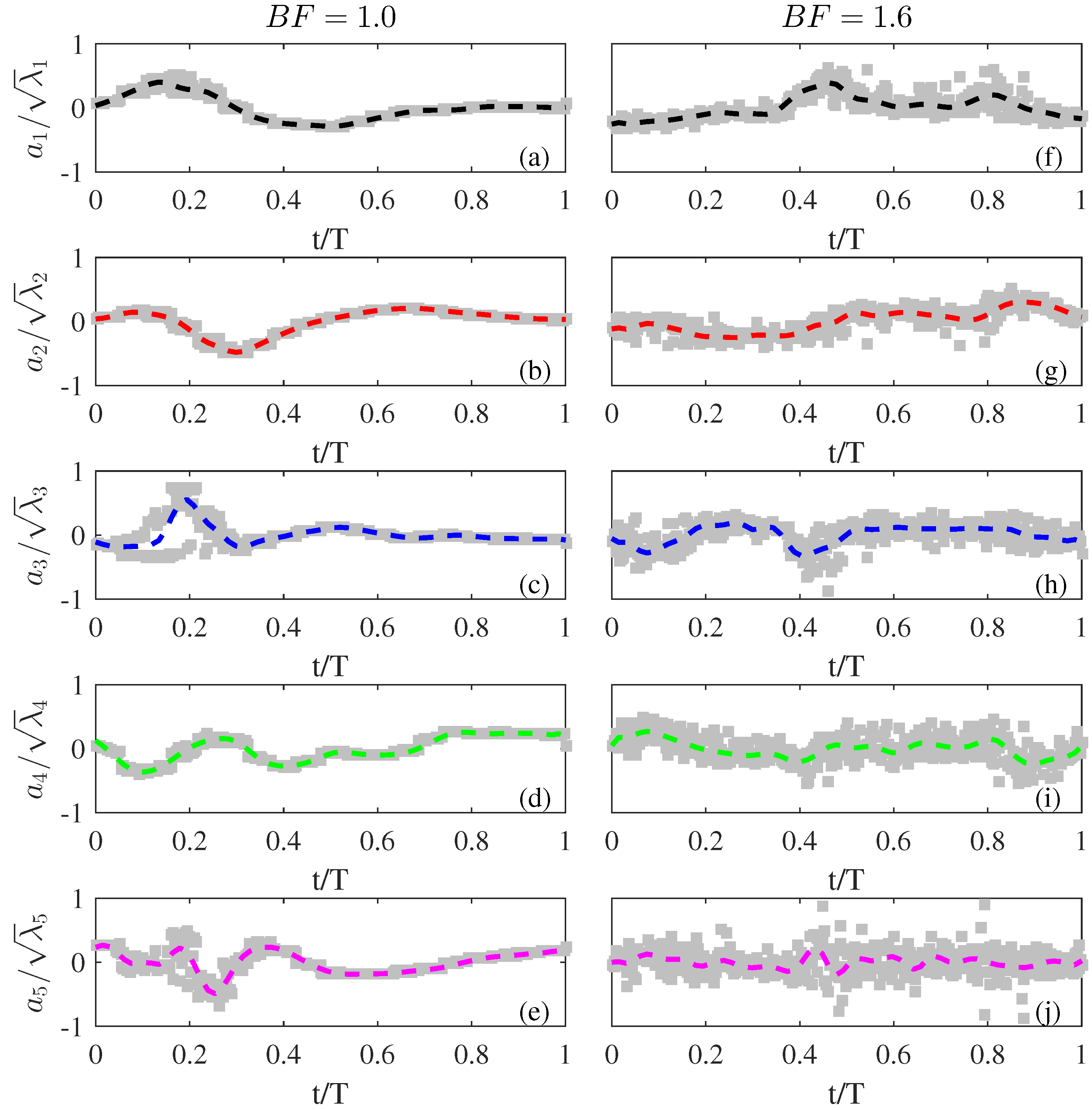
The time-varying coefficients of the POD modes are analyzed to learn about the interaction among various POD modes at different points in the flow cycle. This insight is important since the shape of the POD modes provide spatial information and their respective time-varying coefficients provide temporal information for low-order reconstructions of the flow field at a given time instance. The s are determined by projecting the velocity field at a given time instance on the POD modes (see Equation (10)). The obtained values were normalized by the square root of their respective energies (i.e., ). For each sub-figure, values were sequenced to a single flow cycle using the hardware synchronization approach where time information of the coefficients was determined by correlating the PIV trigger and the piston position from the experiments (see Section 2.3). Thus, the plots contained the scatter plot for each time-varying coefficient, and a spline curve fit operation was performed to determine a mathematical relationship for each coefficient. For brevity, only the results for and at different are shown here to illustrate the interaction of values for these scenarios.
Figure 9a–e contains the phase portrait plots for using the first five for , while Figure 9f–j contains the first five values for . From these figures, it can be observed that there is significant variation in the time-varying coefficients trend in a single flow cycle for both cases. There are points in the cycle when certain time-varying coefficients are close to zero value, suggesting that contributions from those POD modes to the flow field are minimal, and the other modes may play a bigger role in describing the flow behavior at that time. These figures clearly show the difference in time-varying coefficients between the and cases. This suggests that overall temporal flow behavior in these two aneurysm models will be different for the same inflow conditions.
3.5. POD Low-Order Reconstruction
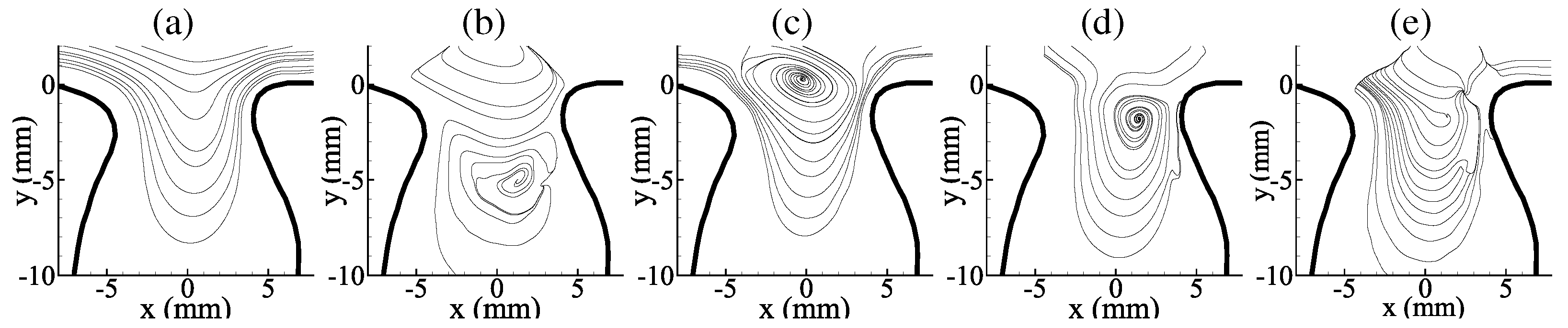
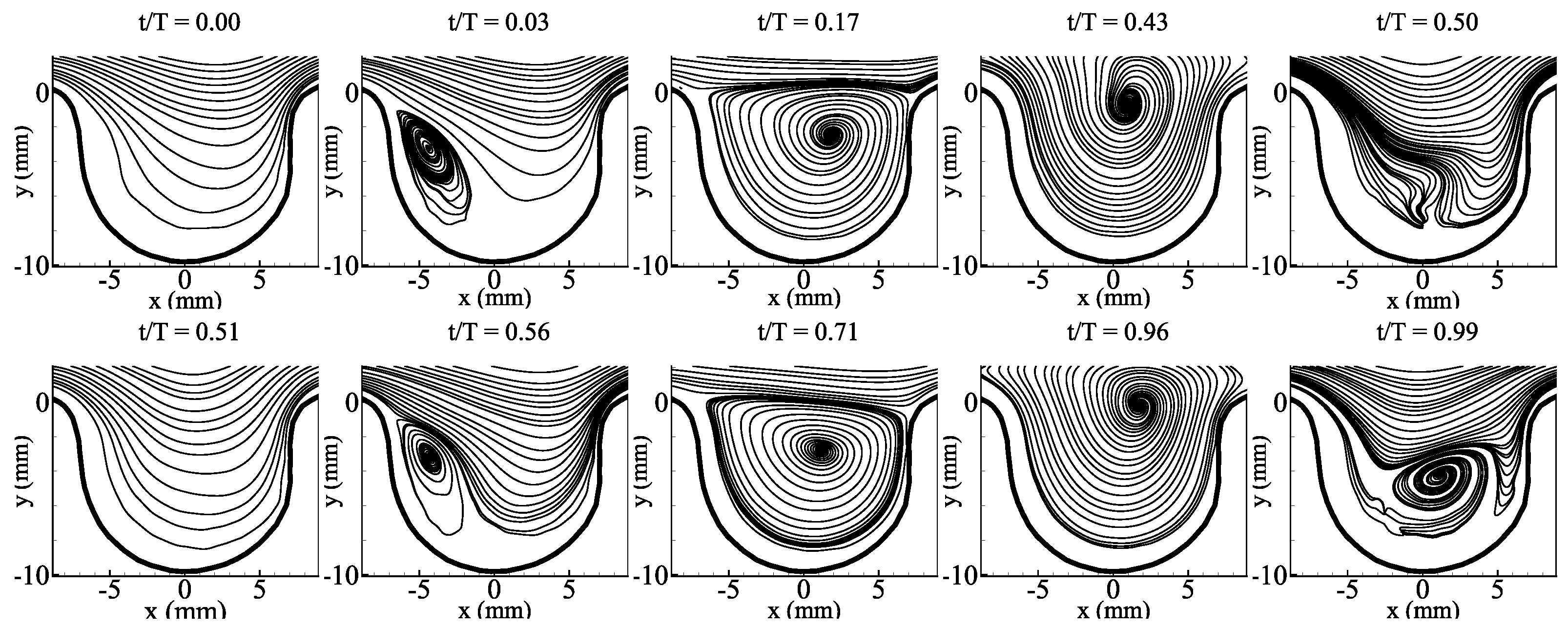
The POD modes, energies, and time-varying coefficient results from previous sections are combined together to create a low-order reconstruction for each flow condition. The low-order reconstruction allows obtaining insight on the dynamics of the flow through the interaction of POD mode shapes and coefficients. The reconstruction results used a mathematical model to create an accurate representation of the flow field. To create a low-order reconstruction model, Equation (3) is used for selected N POD modes. The number of modes was determined by comparing POD reconstructions relative to PIV images that sufficiently capture large-scale features (not shown in this paper). This corresponded to the first three POD modes for scenarios and the first five POD modes for scenarios for . For , five POD modes were used for scenarios while ten POD modes were used for flow scenarios. Here, the results were presented to focus on the similarities and differences observed between the flow scenarios and morphologies. A detailed discussion of POD reconstruction results for can be found in Yu et al. [23].
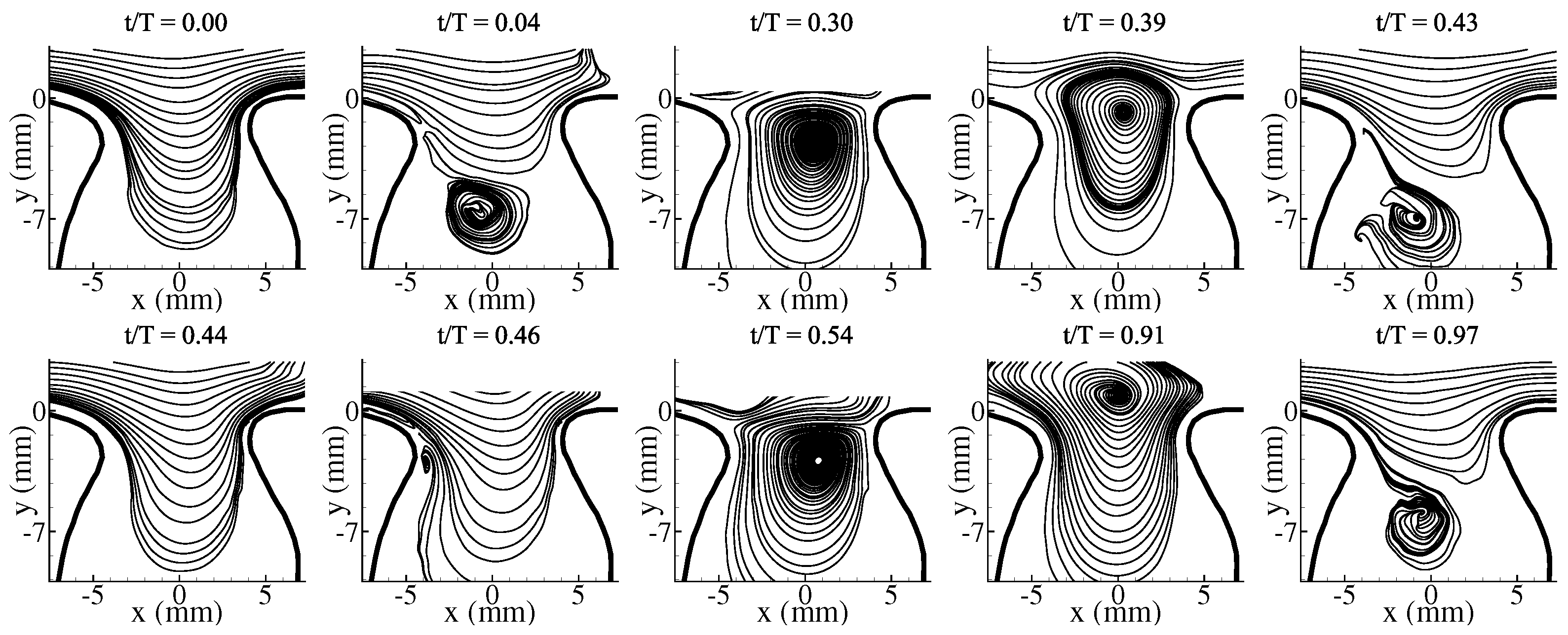
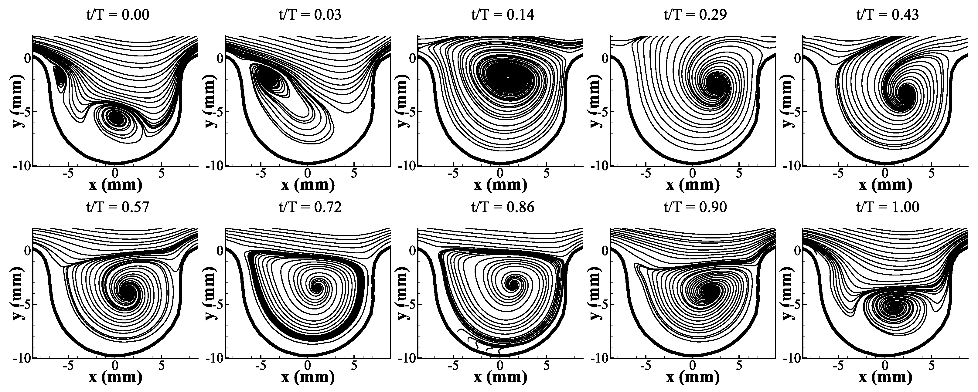
The low-order velocity reconstructions for the model with and inflow condition of and are shown in Figure 10. As observed in the figure, the vortical structure convects towards the center of the aneurysm and then out for the first half of the cycle. This process is repeated for the second half of the flow cycle, and the vortical structure follows the same path trajectory. For the model with and inflow condition of and , the low-order reconstructions are able to capture the initiation, growth, and convection of the vortical structure in the flow cycle, as shown in Figure 11. It is interesting to note here that we observe an elongation of the vortical structure as it convects out of the aneurysm sac, which was not observed for the case. For the model with , the vortical structure mostly spanned the neck and middle portion of the aneurysm model, but the vortical structure was able to cover the entire aneurysm sac. A similar trend in vortical structure formation and movement was observed for and for the models with and .
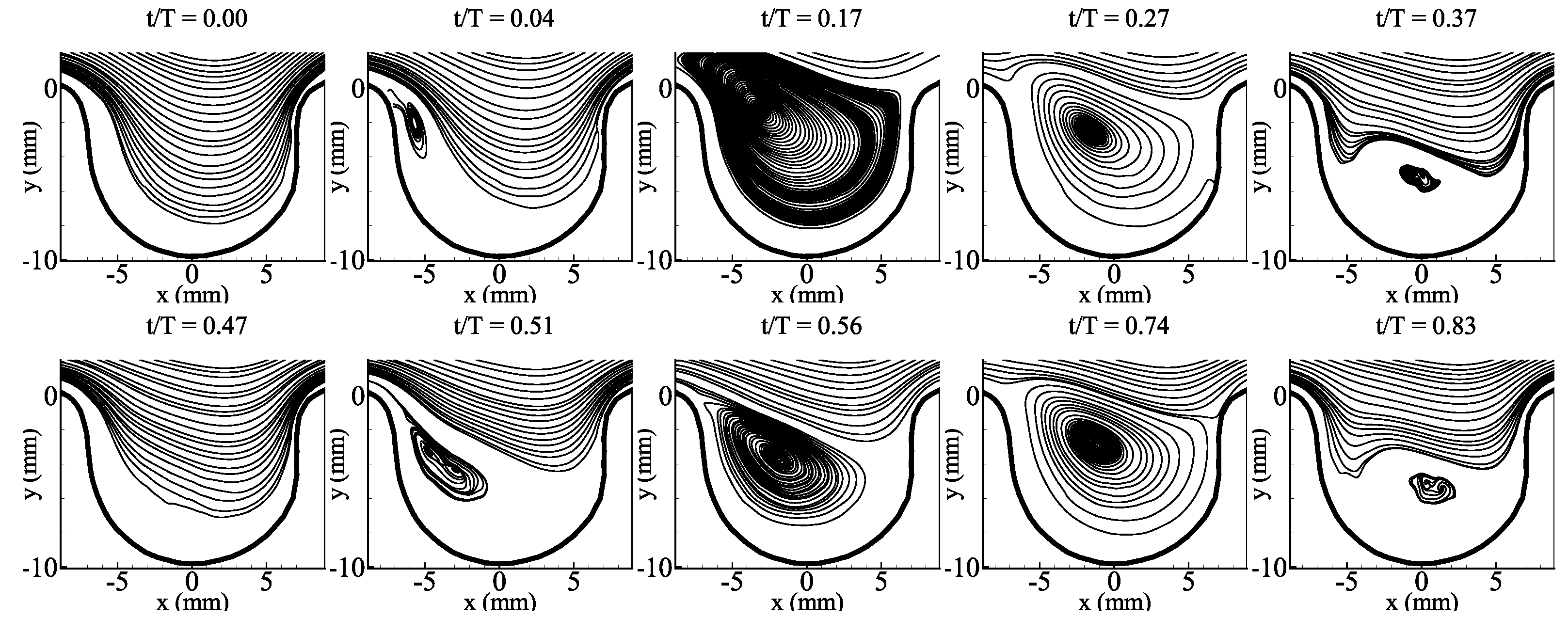
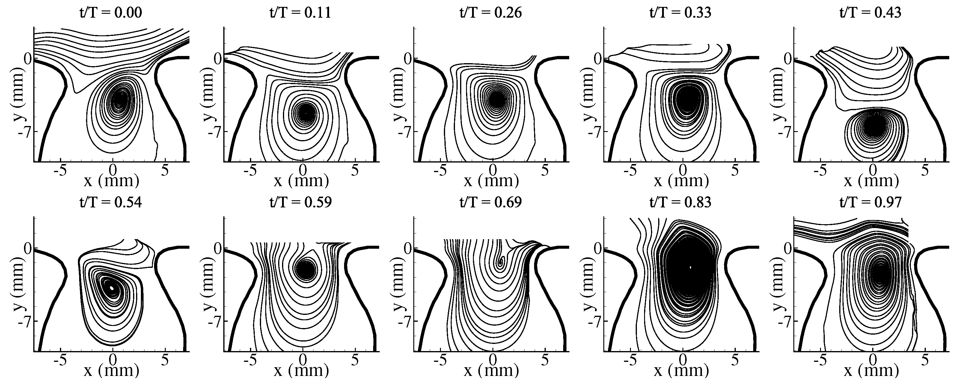
The low-order reconstructions for the model with and inflow conditions of and are shown in Figure 12. As observed in the figure, the vortex structure forms near the proximal side of the aneurysm, moves towards the distal side, and convects down into the aneurysm sac, where it dissipates, which is in contrast with the inflow condition of and and 270 for the model with case, where the vortical structure convects outside the aneurysm sac. Similarly to prior low-order reconstructions, we see the process repeated for the latter half of the cycle. With the change in to 1.6 and for the same inflow conditions (i.e., and ), the vortical structure forms near the proximal side, moves out of the aneurysm through the neck opening, and returns to the aneurysm sac, where it oscillates vertically (see Figure 13).
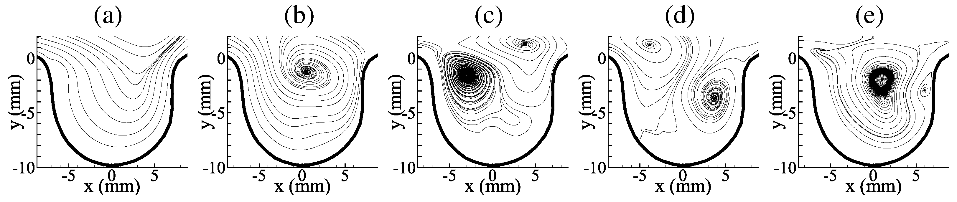
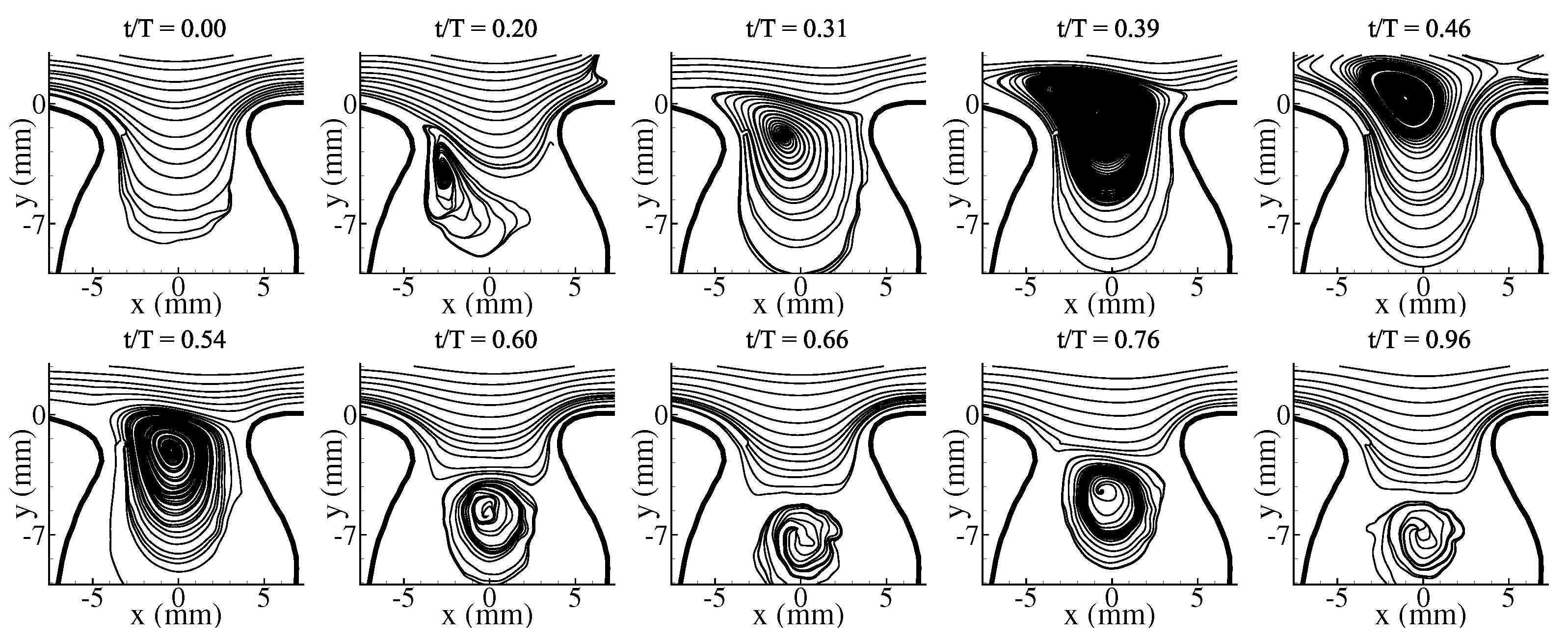
The next set of reconstructions was performed for inflow conditions of and for both models (i.e., and ), as shown in Figure 14 and Figure 15, respectively. It is evident from these figures that, at higher , the flow is significantly different for both models. For the model with , a primary vortical structure along with a secondary vortical is observed ( see Figure 14). It is also evident in these reconstructions that the secondary vortical structure merges with the primary vortical structure, forming a single vortex structure. With changes in morphology to (Figure 15), only a single vortical structure was observed in the aneurysm. This vortical structure moves back and forth between the aneurysm neck opening and the center of the aneurysm sac.
POD reconstructions were able to capture the flow evolution in the aneurysm sac at different inflow conditions. Results from POD provided information on the impact of inflow conditions and model geometry on the flow’s features. The low-order reconstruction captured vortex formation, evolution, and convection.
4. Conclusions
POD was used to quantify the coherent flow structures in aneurysm flow for two selected geometries. Two-dimensional PIV measurements were performed for two rigid aneurysm models to capture the flow field evolution at different inflow scenarios. PIV measurements were performed at inflow conditions of = 2–5 and = 50–270 for two models with and . A SuperPump system was used to control the inflow conditions, and it was synchronized with the PIV system to determine the phase in the flow cycle. The modes, energies, and time-varying coefficients at different inflow scenarios were extracted using POD. Low-order velocity field reconstruction at different inflow conditions was performed to quantify flow behavior, such as the vortex formation process and movement for the studied models and inflow conditions.
The average flow field results highlighted the differences in the mean flow structure present in the aneurysm at different inflow scenarios. The results showed that and had more significant influence on the averaged flow structures than the variation in . POD analysis provided detailed insight into the complex flow behavior in the aneurysm. The POD mode shape results changed with varying inflow conditions and geometries and provided spatial descriptions on the flow structures. POD energy results showed that different modes contained different energy levels, and the first ten POD modes can capture at least 80% of the fluctuating energy in the flow. The time-varying coefficients’ results showed the interaction among the modes, and this was highlighted with a complex interplay of modes for flow scenarios than . The POD modes, energies, and coefficients allowed low-order flow modeling to capture the complex flow behavior in the aneurysm.
The low-order flow reconstruction using appropriate amount of modes provided an accurate temporal representation of the large-scale structures in the flow field at different inflow conditions such as , , and model geometries (i.e., two ). The flow field at each phase of the flow cycle was obtained using POD modes and their time-varying coefficients. For fixed scenarios, the vortex formation process and movement remained relatively similar across different and . The formation of the vortex was initiated from the proximal side, which exited the aneurysm opening and was followed by its return and dissipation processes. This vortical formation and movement occurred between and , and this process repeated itself for the rest of the flow cycle. Meanwhile, for scenarios, different vortical structure behavior was observed at different and . In this study, we observed a single vortical structure in the aneurysm or a primary vortex merging together with a secondary vortex forming a single vortex at a latter time in the cycle.
POD provides a method for analyzing complex flow phenomena in great detail. It can be used to study a variety of unsteady, physiological flows to understand the behavior of energetic flow structures. POD also provides an alternative approach to create mathematical models and to examine flow evolution at any time step. This method can be more advantageous for a researcher than performing phase-locked measurements, which can be time consuming and require extensive hardware synchronization. With POD, pertinent information can be extracted with an appropriate number of PIV images. Lastly, POD can aid researchers in comparing numerical and computational data as well as quantification across different inflow scenarios.
Author Contributions
P.Y. and V.D. contributed equally to the manuscript. All authors have read and agreed to the published version of the manuscript.
Funding
This research received no external funding.
Institutional Review Board Statement
Not applicable.
Informed Consent Statement
Not applicable.
Data Availability Statement
Data are available upon request from the corresponding author.
Conflicts of Interest
The authors declare no conflict of interest.
Nomenclature
The following abbreviations, symbols, and markings are used in this manuscript:
| Computational Fluid Dynamics; | |
| Pipe diameter (m); | |
| Particle Image Velocimetry; | |
| Proper Orthogonal Decomposition; | |
| Spatial velocity correlation matrix; | |
| Peak Reynolds number; | |
| t | Time (s); |
| T | Time period (s); |
| Velocity vector; | |
| Velocity component in x-direction (m/s); | |
| Velocity component in y-direction (m/s); | |
| Maximum centerline velocity in the pipe (m/s); | |
| Cartesian coordinates; | |
| Womersley number; | |
| Blood kinematic viscosity (m2/s); | |
| Kinematic viscosity (m2/s); | |
| Blood density (kg/m3); | |
| Fluid density (kg/m3); | |
| Angular frequency (rad/s); | |
| ith POD mode; | |
| Streamwise component of ith POD mode; | |
| Transverse component of ith POD mode; | |
| Domain of interest; | |
| Energy captured by ith POD mode; | |
| ⊗ | Tensor product; |
| Ensemble averaging. |
References
- Wiebers, D.O.; Torner, J.C.; Meissner, I. Impact of unruptured intracranial aneurysms on public health in the United States. Stroke 1992, 23, 1416–1419. [Google Scholar] [CrossRef] [Green Version]
- Vega, C.; Kwoon, J.V.; Lavine, S.D. Intracranial aneurysms: Current evidence and clinical practice. Am. Fam. Physician 2002, 66, 601–610. [Google Scholar] [PubMed]
- Brisman, J.L.; Song, J.K.; Newell, D.W. Cerebral aneurysms. N. Engl. J. Med. 2006, 355, 928–939. [Google Scholar] [CrossRef] [Green Version]
- Lasheras, J.C. The biomechanics of arterial aneurysms. Annu. Rev. Fluid Mech. 2007, 39, 293–319. [Google Scholar] [CrossRef] [Green Version]
- Cebral, J.R.; Raschi, M. Suggested connections between risk factors of intracranial aneurysms: A review. Ann. Biomed. Eng. 2013, 41, 1366–1383. [Google Scholar] [CrossRef] [PubMed]
- Burleson, A.C.; Strother, C.M.; Turitto, V.T. Computer modeling of intracranial saccular and lateral aneurysms for the study of their hemodynamics. Neurosurgery 1995, 37, 774–784. [Google Scholar] [CrossRef] [PubMed]
- Tateshima, S.; Murayama, Y.; Villablanca, J.P.; Morino, T.; Takahashi, H.; Yamauchi, T.; Tanishita, K.; Viñuela, F. Intraaneurysmal flow dynamics study featuring an acrylic aneurysm model manufactured using a computerized tomography angiogram as a mold. J. Neurosurg. 2001, 95, 1020–1027. [Google Scholar] [CrossRef]
- Ujiie, H.; Tachi, H.; Hiramatsu, O.; Hazel, A.L.; Matsumoto, T.; Ogasawara, Y.; Nakajima, H.; Hori, T.; Takakura, K.; Kajiya, F. Effects of size and shape (aspect ratio) on the hemodynamics of saccular aneurysms: A possible index for surgical treatment of intracranial aneurysms. Neurosurgery 1999, 45, 119–130. [Google Scholar]
- Sekhar, L.N.; Heros, R.C. Origin, growth, and rupture of saccular aneurysms: A review. Neurosurgery 1981, 8, 248–260. [Google Scholar] [CrossRef]
- Hoi, Y.; Meng, H.; Woodward, S.H.; Bendok, B.R.; Hanel, R.A.; Guterman, L.R.; Hopkins, L.N. Effects of arterial geometry on aneurysm growth: Three-dimensional computational fluid dynamics study. J. Neurosurg. 2004, 101, 676–681. [Google Scholar] [CrossRef]
- Ionita, C.N.; Hoi, Y.; Meng, H.; Rudin, S. Particle image velocimetry (PIV) evaluation of flow modification in aneurysm phantoms using asymmetric stents. In Proceedings of the Medical Imaging 2004: Physiology, Function, and Structure from Medical Images, San Diego, CA, USA, 15–17 February 2004; International Society for Optics and Photonics: Bellingham, WA, USA, 2004; Volume 5369, pp. 295–307. [Google Scholar]
- Bouillot, P.; Brina, O.; Ouared, R.; Lovblad, K.; Pereira, V.M.; Farhat, M. Multi-time-lag PIV analysis of steady and pulsatile flows in a sidewall aneurysm. Exp. Fluids 2014, 55, 1746. [Google Scholar] [CrossRef] [Green Version]
- Bluestein, D.; Niu, L.; Schoephoerster, R.; Dewanjee, M. Steady flow in an aneurysm model: Correlation between fluid dynamics and blood platelet deposition. J. Biomech. Eng. 1996, 118, 280–286. [Google Scholar] [CrossRef] [PubMed]
- Lieber, B.B.; Livescu, V.; Hopkins, L.; Wakhloo, A.K. Particle image velocimetry assessment of stent design influence on intra-aneurysmal flow. Ann. Biomed. Eng. 2002, 30, 768–777. [Google Scholar] [CrossRef] [PubMed]
- Budwig, R.; Elger, D.; Hooper, H.; Slippy, J. Steady flow in abdominal aortic aneurysm models. J. Biomech. Eng. 1993, 115, 418–423. [Google Scholar] [CrossRef] [PubMed]
- Fukushima, T.; Matsuzawa, T.; Homma, T. Visualization and finite element analysis of pulsatile flow in models of the abdominal aortic aneurysm. Biorheology 1989, 26, 109–130. [Google Scholar] [CrossRef]
- Egelhoff, C. A model study of pulsatile flow regimes in abdominal aortic aneurysms. In Proceedings of the ASME FEDSM97-34-31, ASME Fluids Engineering Division Summer Division Meeting, Vancouver, BC, Canada, 22–26 June 1997. [Google Scholar]
- Taylor, T.W.; Yamaguchi, T. Three-dimensional simulation of blood flow in an abdominal aortic aneurysm—Steady and unsteady flow cases. J. Biomech. Eng. 1994, 116, 89–97. [Google Scholar] [CrossRef]
- Gobin, Y.; Counord, J.; Flaud, P.; Duffaux, J. In vitro study of haemodynamics in a giant saccular aneurysm model: Influence of flow dynamics in the parent vessel and effects of coil embolisation. Neuroradiology 1994, 36, 530–536. [Google Scholar] [CrossRef]
- Yu, S.; Zhao, J. A steady flow analysis on the stented and non-stented sidewall aneurysm models. Med. Eng. Phys. 1999, 21, 133–141. [Google Scholar] [CrossRef]
- Le, T.B.; Borazjani, I.; Sotiropoulos, F. Pulsatile flow effects on the hemodynamics of intracranial aneurysms. J. Biomech. Eng. 2010, 132, 111009. [Google Scholar] [CrossRef]
- Yu, P.; Durgesh, V. Experimental Study of Large-Scale Flow Structures in an Aneurysm. In Proceedings of the Fluids Engineering Division Summer Meeting, Montreal, QC, Canada, 15–20 July 2018; Volume 51555, p. V001T02A009. [Google Scholar]
- Yu, P.; Durgesh, V.; Xing, T.; Budwig, R. Application of Proper Orthogonal Decomposition to Study Coherent Flow Structures in a Saccular Aneurysm. J. Biomech. Eng. 2021, 143, 061008. [Google Scholar] [CrossRef]
- Yu, P.; Durgesh, V. Application of Dynamic Mode Decomposition to Study Temporal Flow Behavior in a Saccular Aneurysm. J. Biomech. Eng. 2022, 144, 51002. [Google Scholar] [CrossRef] [PubMed]
- Asgharzadeh, H.; Borazjani, I. A non-dimensional parameter for classification of the flow in intracranial aneurysms. I. Simplified geometries. Phys. Fluids 2019, 31, 031904. [Google Scholar] [CrossRef] [PubMed]
- Asgharzadeh, H.; Asadi, H.; Meng, H.; Borazjani, I. A non-dimensional parameter for classification of the flow in intracranial aneurysms. II. Patient-specific geometries. Phys. Fluids 2019, 31, 031905. [Google Scholar] [CrossRef] [PubMed]
- Asgharzadeh, H.; Borazjani, I. Effects of Reynolds and Womersley numbers on the hemodynamics of intracranial aneurysms. Comput. Math. Methods Med. 2016, 2016, 7412926. [Google Scholar] [CrossRef] [Green Version]
- Lumley, J.L. The structure of inhomogeneous turbulent flows. In Atmospheric Turbulence and Radio Wave Propagation; Yaglom, A.M., Tartarsky, V.I., Eds.; Nauka: Tokyo, Japan, 1967; pp. 166–177. [Google Scholar]
- Rowley, C.; Colonius, T.; Murray, R. POD based models of self-sustained oscillations in the flow past an open cavity. In Proceedings of the 6th Aeroacoustics Conference and Exhibit, Lahaina, HI, USA, 12–14 June 2000; p. 1969. [Google Scholar]
- Berkooz, G.; Holmes, P.; Lumley, J.L. The proper orthogonal decomposition in the analysis of turbulent flows. Annu. Rev. Fluid Mech. 1993, 25, 539–575. [Google Scholar] [CrossRef]
- Graftieaux, L.; Michard, M.; Grosjean, N. Combining PIV, POD and vortex identification algorithms for the study of unsteady turbulent swirling flows. Meas. Sci. Technol. 2001, 12, 1422. [Google Scholar] [CrossRef]
- Chen, H.; Selimovic, A.; Thompson, H.; Chiarini, A.; Penrose, J.; Ventikos, Y.; Watton, P.N. Investigating the influence of haemodynamic stimuli on intracranial aneurysm inception. Ann. Biomed. Eng. 2013, 41, 1492–1504. [Google Scholar] [CrossRef]
- Byrne, G.; Mut, F.; Cebral, J. Quantifying the large-scale hemodynamics of intracranial aneurysms. Am. J. Neuroradiol. 2014, 35, 333–338. [Google Scholar] [CrossRef] [Green Version]
- Daroczy, L.; Abdelsamie, A.; Janiga, G.; Thevenin, D. State Detection and Hybrid Simulation of Biomedical Flows. In Proceedings of the Tenth International Symposium on Turbulence and Shear Flow Phenomena, Chicago, IL, USA, 7–9 July 2017; Begel House Inc.: Danbury, CT, USA, 2017. [Google Scholar]
- Janiga, G. Quantitative assessment of 4D hemodynamics in cerebral aneurysms using proper orthogonal decomposition. J. Biomech. 2019, 82, 80–86. [Google Scholar] [CrossRef]
- Bluestein, D.; Moore, J.E. Biofluids educational issues: An emerging field aims to define its next generation. Ann. Biomed. Eng. 2005, 33, 1674–1680. [Google Scholar] [CrossRef]
- Cebral, J.R.; Castro, M.A.; Burgess, J.E.; Pergolizzi, R.S.; Sheridan, M.J.; Putman, C.M. Characterization of cerebral aneurysms for assessing risk of rupture by using patient-specific computational hemodynamics models. Am. J. Neuroradiol. 2005, 26, 2550–2559. [Google Scholar] [PubMed]
- Shojima, M.; Oshima, M.; Takagi, K.; Torii, R.; Nagata, K.; Shirouzu, I.; Morita, A.; Kirino, T. Role of the bloodstream impacting force and the local pressure elevation in the rupture of cerebral aneurysms. Stroke 2005, 36, 1933–1938. [Google Scholar] [CrossRef] [PubMed] [Green Version]
- Tateshima, S.; Tanishita, K.; Omura, H.; Villablanca, J.; Vinuela, F. Intra-aneurysmal hemodynamics during the growth of an unruptured aneurysm: In vitro study using longitudinal CT angiogram database. Am. J. Neuroradiol. 2007, 28, 622–627. [Google Scholar] [PubMed]
- Bluestein, D.; Dumont, K.; De Beule, M.; Ricotta, J.; Impellizzeri, P.; Verhegghe, B.; Verdonck, P. Intraluminal thrombus and risk of rupture in patient specific abdominal aortic aneurysm–FSI modelling. Comput. Methods Biomech. Biomed. Eng. 2009, 12, 73–81. [Google Scholar] [CrossRef]
- Watton, P.; Ventikos, Y. Modelling evolution of saccular cerebral aneurysms. J. Strain Anal. Eng. Des. 2009, 44, 375–389. [Google Scholar] [CrossRef]
- Torii, R.; Oshima, M.; Kobayashi, T.; Takagi, K.; Tezduyar, T.E. Influencing factors in image-based fluid–structure interaction computation of cerebral aneurysms. Int. J. Numer. Methods Fluids 2011, 65, 324–340. [Google Scholar] [CrossRef]
- Usmani, A.Y.; Muralidhar, K. Flow in an intracranial aneurysm model: Effect of parent artery orientation. J. Vis. 2018, 21, 795–818. [Google Scholar] [CrossRef]
- Li, Z.; Hu, L.; Chen, C.; Wang, Z.; Zhou, Z.; Chen, Y. Hemodynamic performance of multilayer stents in the treatment of aneurysms with a branch attached. Sci. Rep. 2019, 9, 10193. [Google Scholar] [CrossRef] [Green Version]
- Saqr, K.M.; Rashad, S.; Tupin, S.; Niizuma, K.; Hassan, T.; Tominaga, T.; Ohta, M. What does computational fluid dynamics tell us about intracranial aneurysms? A meta-analysis and critical review. J. Cereb. Blood Flow Metab. 2020, 40, 1021–1039. [Google Scholar] [CrossRef]
- Fahrig, R.; Nikolov, H.; Fox, A.; Holdsworth, D. A three-dimensional cerebrovascular flow phantom. Med. Phys. 1999, 26, 1589–1599. [Google Scholar] [CrossRef]
- Hopkins, L.; Kelly, J.; Wexler, A.; Prasad, A. Particle image velocimetry measurements in complex geometries. Exp. Fluids 2000, 29, 91–95. [Google Scholar] [CrossRef]
- Ugron, Á.; Farinas, M.I.; Kiss, L.; Paál, G. Unsteady velocity measurements in a realistic intracranial aneurysm model. Exp. Fluids 2012, 52, 37–52. [Google Scholar] [CrossRef]
- Geoghegan, P.; Buchmann, N.; Spence, C.; Moore, S.; Jermy, M. Fabrication of rigid and flexible refractive-index-matched flow phantoms for flow visualisation and optical flow measurements. Exp. Fluids 2012, 52, 1331–1347. [Google Scholar] [CrossRef]
- Le, T.B.; Troolin, D.R.; Amatya, D.; Longmire, E.K.; Sotiropoulos, F. Vortex phenomena in sidewall aneurysm hemodynamics: Experiment and numerical simulation. Ann. Biomed. Eng. 2013, 41, 2157–2170. [Google Scholar] [CrossRef]
- Yong, K.W.; Janmaleki, M.; Pachenari, M.; Mitha, A.P.; Sanati-Nezhad, A.; Sen, A. Engineering a 3D human intracranial aneurysm model using liquid-assisted injection molding and tuned hydrogels. Acta Biomater. 2021, 136, 266–278. [Google Scholar] [CrossRef] [PubMed]
- Budwig, R. Refractive index matching methods for liquid flow investigations. Exp. Fluids 1994, 17, 350–355. [Google Scholar] [CrossRef]
- Bai, K.; Katz, J. On the refractive index of sodium iodide solutions for index matching in PIV. Exp. Fluids 2014, 55, 1704. [Google Scholar] [CrossRef]
- Miller, P.; Danielson, K.; Moody, G.; Slifka, A.; Drexler, E.; Hertzberg, J. Matching index of refraction using a diethyl phthalate/ethanol solution for in vitro cardiovascular models. Exp. Fluids 2006, 41, 375–381. [Google Scholar] [CrossRef]
- Adrian, R.J. Particle-imaging techniques for experimental fluid mechanics. Annu. Rev. Fluid Mech. 1991, 23, 261–304. [Google Scholar] [CrossRef]
- Boillot, A.; Prasad, A. Optimization procedure for pulse separation in cross-correlation PIV. Exp. Fluids 1996, 21, 87–93. [Google Scholar] [CrossRef]
- Meinhart, C.D.; Wereley, S.T.; Santiago, J.G. A PIV algorithm for estimating time-averaged velocity fields. J. Fluids Eng. 2000, 122, 285–289. [Google Scholar] [CrossRef] [Green Version]
- Ku, D.N. Blood flow in arteries. Annu. Rev. Fluid Mech. 1997, 29, 399–434. [Google Scholar] [CrossRef]
- Ma, B.; Harbaugh, R.E.; Raghavan, M.L. Three-dimensional geometrical characterization of cerebral aneurysms. Ann. Biomed. Eng. 2004, 32, 264–273. [Google Scholar] [CrossRef] [PubMed]
- Steiger, H.; Poll, A.; Liepsch, D.; Reulen, H.J. Haemodynamic stress in lateral saccular aneurysms. Acta Neurochir. 1987, 86, 98–105. [Google Scholar] [CrossRef] [PubMed]
- Womersley, J.R. Method for the calculation of velocity, rate of flow and viscous drag in arteries when the pressure gradient is known. J. Physiol. 1955, 127, 553–563. [Google Scholar] [CrossRef]
- Steiger, H.J.; Poll, A.; Liepsch, D.; Reulen, H.J. Basic flow structure in saccular aneurysms: A flow visualization study. Heart Vessel. 1987, 3, 55–65. [Google Scholar] [CrossRef]
- Liou, T.M.; Liou, S.N. A review on in vitro studies of hemodynamic characteristics in terminal and lateral aneurysm models. Proc. Natl. Sci. Counc. Repub. China Part B Life Sci. 1999, 23, 133. [Google Scholar]
- White, F.M.; Corfield, I. Viscous Fluid Flow; McGraw-Hill: New York, NY, USA, 2006; Volume 3. [Google Scholar]
- Holman, R.; Utturkar, Y.; Mittal, R.; Smith, B.L.; Cattafesta, L. Formation criterion for synthetic jets. AIAA J. 2005, 43, 2110–2116. [Google Scholar] [CrossRef] [Green Version]
- Sirovich, L. Turbulence and the dynamics of coherent structures. I. Coherent structures. Q. Appl. Math. 1987, 45, 561–571. [Google Scholar] [CrossRef] [Green Version]
- Holmes, P.; Lumley, J.L.; Berkooz, G.; Rowley, C.W. Turbulence, Coherent Structures, Dynamical Systems and Symmetry; Cambridge University Press: Cambridge, MA, USA, 2012. [Google Scholar]
- Durgesh, V.; Naughton, J. Multi-time-delay LSE-POD complementary approach applied to unsteady high-Reynolds-number near wake flow. Exp. Fluids 2010, 49, 571–583. [Google Scholar] [CrossRef]
Figure 1.
Critical features of the idealized, saccular, aneurysm model for (a) and (b) .

Figure 2.
Key components of 2D PIV system for the experimental fluid flow study.

Figure 3.
Average velocity field inside the aneurysm sac for for (a) and , (b) and , (c) and , and (d) and .
Figure 3.
Average velocity field inside the aneurysm sac for for (a) and , (b) and , (c) and , and (d) and .

Figure 4.
POD modes presented as streamlines for , , and . (a) , (b) , (c) , (d) , and (e) .

Figure 5.
POD modes presented as streamlines for , , and . (a) , (b) , (c) , (d) , and (e) .

Figure 6.
POD modes presented as streamlines for , , and . (a) , (b) , (c) , (d) , and (e) .

Figure 7.
POD modes presented as streamlines for , , and . (a) , (b) , (c) , (d) , and (e) .

Figure 8.
Sum of energies for (a) BF = 1.0 and (b) BF = 1.6 at different and .

Figure 9.
Time-varying coefficients – for and . Grey square markers represent experimental data while dashed lines represent curve fit data. (a–e) and (f–j) .
Figure 9.
Time-varying coefficients – for and . Grey square markers represent experimental data while dashed lines represent curve fit data. (a–e) and (f–j) .

Figure 10.
POD low-order reconstruction for , , and for selected time phases. The velocity reconstruction used three POD modes.
Figure 10.
POD low-order reconstruction for , , and for selected time phases. The velocity reconstruction used three POD modes.

Figure 11.
POD low-order reconstruction for , , and for selected time phases. The velocity reconstruction used ten POD modes.
Figure 11.
POD low-order reconstruction for , , and for selected time phases. The velocity reconstruction used ten POD modes.

Figure 12.
POD low-order reconstruction for , , and for selected time phases. The velocity reconstruction used five POD modes.
Figure 12.
POD low-order reconstruction for , , and for selected time phases. The velocity reconstruction used five POD modes.

Figure 13.
POD low-order reconstruction for , , and for selected time phases. The velocity reconstruction used five POD modes.
Figure 13.
POD low-order reconstruction for , , and for selected time phases. The velocity reconstruction used five POD modes.

Figure 14.
POD low-order reconstruction for , , and for selected time phases. The velocity reconstruction used five POD modes.
Figure 14.
POD low-order reconstruction for , , and for selected time phases. The velocity reconstruction used five POD modes.

Figure 15.
POD low-order reconstruction for , , and for selected time phases. The velocity reconstruction used ten POD modes.
Figure 15.
POD low-order reconstruction for , , and for selected time phases. The velocity reconstruction used ten POD modes.


Table 1.
Test conditions and measurements performed for and for this study.
| BF | Re | PIV Images | PIV Frame Rate (Hz) | Pump Frequency (Hz) | |
|---|---|---|---|---|---|
| 1.0 | 50 | 2 | 500 | 1.17 | 0.4 |
| 1.0 | 270 | 2 | 500 | 1.17 | 0.4 |
| 1.0 | 50 | 5 | 500 | 1.17 | 2.4 |
| 1.0 | 270 | 5 | 500 | 1.17 | 2.4 |
| 1.6 | 50 | 2 | 500 | 1.17 | 0.4 |
| 1.6 | 270 | 2 | 500 | 1.17 | 0.4 |
| 1.6 | 50 | 5 | 500 | 1.17 | 2.4 |
| 1.6 | 270 | 5 | 500 | 1.17 | 2.4 |
Publisher’s Note: MDPI stays neutral with regard to jurisdictional claims in published maps and institutional affiliations. |
© 2022 by the authors. Licensee MDPI, Basel, Switzerland. This article is an open access article distributed under the terms and conditions of the Creative Commons Attribution (CC BY) license (https://creativecommons.org/licenses/by/4.0/).
Share and Cite
MDPI and ACS Style
Yu, P.; Durgesh, V. Comparison of Flow Behavior in Saccular Aneurysm Models Using Proper Orthogonal Decomposition. Fluids 2022, 7, 123. https://0-doi-org.brum.beds.ac.uk/10.3390/fluids7040123
AMA Style
Yu P, Durgesh V. Comparison of Flow Behavior in Saccular Aneurysm Models Using Proper Orthogonal Decomposition. Fluids. 2022; 7(4):123. https://0-doi-org.brum.beds.ac.uk/10.3390/fluids7040123
Chicago/Turabian StyleYu, Paulo, and Vibhav Durgesh. 2022. "Comparison of Flow Behavior in Saccular Aneurysm Models Using Proper Orthogonal Decomposition" Fluids 7, no. 4: 123. https://0-doi-org.brum.beds.ac.uk/10.3390/fluids7040123