
Modeling Conjugate Heat Transfer in an Anode Baking Furnace Using OpenFoam


1
Faculty of Electrical Engineering, Mathematics and Computer Science, Delft Institute of Applied Mathematics, Technical University of Delft, 2628 CD Delft, The Netherlands
2
Creative Fields Ltd., 10000 Zagreb, Croatia
3
PMSQUARED Engineering s.r.l.s., 09127 Cagliari, Italy
*
Author to whom correspondence should be addressed.
Fluids 2022, 7(4), 124; https://0-doi-org.brum.beds.ac.uk/10.3390/fluids7040124
Submission received: 2 February 2022
/
Revised: 10 March 2022
/
Accepted: 16 March 2022
/
Published: 23 March 2022
(This article belongs to the Special Issue Modeling and Experimental Techniques to Combat Pollutant Emissions from Combustion Systems)
Abstract
:The operation of large industrial furnaces will continue to rely on hydrocarbon fuels in the near foreseeable future. Mathematical modeling and numerical simulation is expected to deliver key insights to implement measures to further reduce pollutant emissions. These measures include the design optimization of the burners, the dilution of oxidizer with exhaust gasses, and the mixing of natural gas with hydrogen. In this paper, we target the numerical simulation of non-premixed turbulent combustion of natural gas in a single heating section of a ring pit anode baking furnace. In previous work, we performed combustion simulations using a commercial flow simulator combined with an open-source package for the three-dimensional mesh generation. This motivates switching to a fully open-source software stack. In this paper, we develop a Reynolds-Averaged Navier-Stokes model for the turbulent flow combined with an infinitely fast mixed-is-burnt model for the non-premixed combustion and a participating media model for the radiative heat transfer in OpenFoam. The heat transfer to the refractory brick lining is taken into account by a conjugate heat transfer model. Numerical simulations provide valuable insight into the heat release and chemical species distribution in the staged combustion process using two burners. Results show that at the operating conditions implemented, higher peak temperatures are formed at the burner closest to the air inlet. This results in a larger thermal nitric-oxide concentration. The inclusion of the heat absorption in the refractory bricks results in a more uniform temperature on the symmetry plane at the center of the section. The peak in thermal nitric-oxides is reduced by a factor of four compared to the model with adiabatic walls.
1. Introduction
This paper is motivated by the wish to reduce the pollutant emission from large industrial furnaces. We target modeling the non-premixed turbulent combustion of natural gas in ring pit furnaces used by our industrial partner AluChemie BV Rotterdam to bake anode blocks. These furnaces are shown in Figure 1. These anodes are used in the production of aluminum. During the electrolysis process, the anodes wear and require regular replacement. The design and operation of anode baking furnaces has attracted recent attention in e.g., [1,2] and references cited therein. These furnaces consist of long parallel masonry refractory walls. The space between the walls is alternatively being used as a flue (or furnace) and as a pit (or space in which the anode blocks are placed). Heating occurs by the non-premixed combustion of natural gas and pre-heated air. The fuel and oxidizer are injected from the top and the side of the flue, respectively. Raw nodes are baked by the indirect heating across the refractory wall. Along the length of the wall, the furnace is subdivided into sections. These sections accommodate the various stages in the anode baking process.
The numerical simulation of the turbulent combustion in anode baking furnaces was pursued in e.g., [1,2,3,4,5,6,7,8] and the references cited therein. These references provide valuable information on the general thermal management and fuel consumption in these furnaces. Modeling the formation of thermal nitric-oxides, however, requires taking detailed information of the design and operation of the furnace into account. In our previous work in collaboration with the company AluChemie BV Rotterdam, we studied a single heating section of the furnace. This section is the hottest and thus most sensitive to the formation of nitric-oxides. In these previous studies [9,10], we used the commercially available Comsol Multiphysics simulation software. The meshes employed in [9,10] were externally generated using the cfMesh mesh generator [11].
In this paper, we replace the commercial CFD software previously used by open-source alternatives. In recent work [12], we developed a Reynolds-average Navier-Stokes mixed-is-burnt combustion model including radiative heat transfer for a single section of the anode baking furnace using OpenFoam [13]. In this reference, we assumed that the furnace walls are thermally insulating. In the anode baking furnace, however, the heat transfer from the flue to the anode blocks occurs indirectly across the refractory lining. Using adiabatic furnace walls, the temperature in the furnace and the thermal nitric-oxide formation in the flue are over-predicted. We therefore wish to replace the adiabatic assumption in the OpenFoam model by a conjugate heat transfer model that allows for heat transfer into the lining.
The scientific contribution we thus wish to pursue is to quantify the effect of adding the conjugate heat transfer to the model developed in [12] in terms of reduction in peak temperature and thermal NO concentration. Simulations results show that the velocity profile on the symmetry plane is hardly effected by replacing the adiabatic wall by the heat transfer into the lining. The temperature is significantly reduced in the second half of the furnace and the temperature is more uniform across the symmetry plane. The peak in thermal nitric-oxide concentration is reduced by a factor of four.
Here, we simplify Dutch natural gas to its main component, i.e., methane [14]. We assume that the combustion reaction is a single step irreversible reaction. The eddy-dissipation model furthermore assumes that the reaction rate is solely determined by the turbulent mixing of the flow only. The simplifications used in this paper might not apply for natural gas from e.g., Northern Africa or Russia. Nor is our approach representative for the use of fuel blends with for instance hydrogen. To model the combustion of these fuels, more detailed chemical reaction mechanisms and more advanced combustion models are required. Multi-step chemical reaction mechanisms capture various fuel components and the intermediate species. Examples of more advanced combustion models than the model used in this paper include the eddy dissipation concept [15], the flamelet-generated manifold model [16], the thickened flame model [17] and the conditional moment closure method [18]. The judicious application of these more advanced combustion model might require adopting turbulence models that are more advanced models than the standard k- model used in this paper. Immediate candidates for such models include the k--SST and the (Delayed) Detached Eddy Simulation (DES) models [19,20]. Having a more detailed model for the turbulence-chemistry interaction in place would allow to explore more detailed models for the turbulence-radiation interaction in a subsequent step. An example of the use of a more detailed radiative heat transfer model on a lab scale furnace furnace is given in [21]. Examples of how detailed radiative transfer computations influence the modeled thermal nitric-oxide concentration are discussed in [22].
The remainder of this paper is structured in four sections as follows. In Section 2, we describe the geometry, the operational conditions and the mesh of a single section of the anode baking under study. In Section 3, we describe the models for the turbulent flow, the non-premixed combustion, the radiative heat transfer by radiation and the conjugate heat transfer through the lining as well as their use in OpenFoam. In Section 4 we describe results obtained for the turbulent viscosity ratio, temperature and chemical species concentrations. In Section 5 we present conclusions.
2. Heating Section of Anode Baking Furnace
In this section, we describe the geometry, the operating conditions and the mesh of a single section of the anode baking furnace under study.
2.1. Computational Domain for Flue and Lining
The computational domain we consider consists of two adjacent cuboidal subdomains. They represent the flue (i.e., the freeboard or the space in which the combustion takes place) and the masonry refractory lining. The anode blocks are not represented in the geometry. Instead, the measured temperature is imposed on the wall separating the refractory wall and the anode block. Physical properties on the lining are listed in Table 1. Both the flue and lining are heigh and wide. The flue and lining are and thick , respectively. The center plane of the flue is shown in Figure 2. Given that the flue is symmetrical with respect to this plane, only half of the flue is represented and symmetry boundary conditions on the center plane are imposed.
Figure 2 shows that flue is a double U-shaped duct. The natural gas combustion occurs staged by via two burners. Each burner is placed on top of the start of each U-shaped duct. Preheated combustion air is injected through the top left inlets, is mixed with the natural gas injected from both burners, travels through both U-shaped ducts and leaves the outlet located at the top-right. Tie-bricks placed in the center of the ducts ensure integrity of structure and uniformity of the flow. Top and bottom by-passes connect the U-shaped ducts and prevent high pressure zones. The geometrical complexity of both burners is reduced by representing the burners as cylindrical pipes. The arrangement of the tie-bricks is such that the jet leaving the first (or left-most) burner is convected by the cross flow of air and impinges on tie-brick further downstream. The jet leaving from the second burner on the other hand is free to pass in between the tie-bricks. The second jet thus travels further into the furnace than the first one. Our numerical simulations will reveal to what extent the aerodynamics and the heat release of both burners are distinct.
The boundary conditions for the inflow of air and natural gas are listed in Table 2. Both burners carry the same mass flow rate of fuel.
2.2. Computational Mesh in Flue and Lining Domain
Numerical simulations in this paper are performed using a cartesian mesh consisting of 670,579 cells. The boundary layers are not resolved. Wall functions are applied instead. The boundary layers thicker than used in previous simulations in [10] allowing the OpenFoam solvers to converge. The smallest edge length of the cells of the mesh in six zones of the computational domain are listed in Table 3. Four views on the mesh are shown in Figure 3. The local refinement around the tie-bricks and underneath the fuel pipe outlets can clearly be seen. The mesh on the fluid domain was extruded to cover the solid domain as shown at the top-right in Figure 3. At the moment, we focus on analyzing the sensitivity of various model components for the turbulent flow, the combustion and the radiative heat transfer on the mesh considered. We plan to perform a mesh sensitivity study in a later stage of the research. Such a study is computationally expensive in part due to the lack for fast iterative solvers for the large linear systems.
3. Modeling Non-Premixed Turbulent Combustion and Conjugate Heat Transfer in OpenFoam
In this section, we present the model for the non-premixed turbulent combustion in the furnace that we intend to solve numerically using OpenFoam. This model consists of a sub-model for the fluid and solid subdomain. The former consists of three components. The first component is a formulation for the non-isothermal turbulent flow of the mixture of pre-heated air and gaseous fuel. We resort to an unsteady formulation to facilitate handling non-linearities numerically using time-stepping. The second is a formulation for the transport by diffusion and by convection of the individual chemical species. The transport equations include sink and source terms for the depletion of oxidizer and fuel and the creation of combustion products, respectively. The third is a formulation for the radiative heat transport in participating media. The sub-model for the solid describes conductive heat transfer from the hot gasses into the masonry brick lining. This transfer is constrained that the temperature imposed on the outside wall. The fluid and solid sub-models are coupled by interface conditions on the shared boundary. The thermal nitric-oxide mass fraction is computed is post-processing stage. Additional information on the modeling of turbulent combustion and pollutant formation can be found in references such as e.g., [23,24,25]. For details on the modeling of radiative heat transfer and conjugate heat transfer we refer to [22,26], respectively.
We denote by and the molecular viscosity and the molecular thermal conductivity of the gas mixture. Modeling of combustion requires tracking the individual chemical species. We denote their mass fraction as for . We will assume that the heat capacity at constant pressure and the thermal absorption coefficient of the gas mixture depends on the temperature and the species mass fractions. We will denote them by and , respectively. The heat capacity is computed as the mass fraction weighted average
where the heat capacity for species s is a polynomial in T with coefficients that interpolate measured data. These coefficients can be found in the tabulated in the JANNAF tables. Similarly, the thermal absorption coefficient is computed using a weighted sum of grey gasses (WSSG) that models the temperature dependence of the spectral properties of HO and CO.
The Mach number of the flow of the gas mixture in the fluid domain remains bounded by 0.3. The assumption of an incompressible flow model is thus justified. We adopt an unsteady Reynolds-Averaged model with Favre averaging closed by the standard k- two-equation turbulence model for the turbulent kinetic energy k and the eddy dissipation rate , respectively. Let denote the Reynolds-averaged mass density. Using k and , the turbulent mixing time scale , the turbulent eddy viscosity and the turbulent kinematic viscosity are defined as
respectively. is a model constant equal to .
We assume that the combustion occurs in a regime in which diffusion flames with thin reaction fronts are formed. In this regime, the turbulent mixing time scale dominates the chemical time scale. The Damkohler number is thus much larger than one. The eddy dissipation model for combustion exploits the separation of mixing and reaction time scales. It assumes that the chemical reaction rate for the fuel (in ) is proportional to minimum of the mass fraction of fuel and oxidizer. In OpenFoam-v2012 (see Line 100-103 of /src/combustionModels/eddyDissipationModelBase/eddyDissipationModelBase.C of https://develop.openfoam.com/Development/openfoam/-/blob/OpenFOAM-v2012 accessed on 1 March 2022), this model is implemented as
where , and s are the mass fraction of the fuel, the mass fraction of the oxidizer and the stochiometric oxygen-to-fuel mass ratio, respectively. In regions in which the flow is laminar, the turbulent time scale is larger than the laminar diffusion time scale. In laminar flow regions, the time scale in the right-hand side of (3) is given by the smallest of both and defined by
where is the diameter of the cell of the mesh. The quantities and are model constants. Unlike in the classical formulation originally proposed in [27], the definition in (3) does not take the mass fraction of the combustion products is not taken into account. In our simulations, we observe that the value of peak temperature and therefore of the thermal NO concentration is sensitive to the values of and . To obtain closest resemblance to the standard eddy dissipation model possible, we set set and . We simplify Dutch natural gas to methane as its main component. We adapt the single step irreversible global reaction mechanism
which has an enthalpy of combustion equal to of CH. We thus need to track the mass fraction of chemical species. The presence of the inert N2 facilitates enforcing numerically that the mass fractions sum up to one.
Various models that capture the radiative heat transfer to various degrees of accuracy are available in the literature. The P1-model requires solving a non-linear diffusion equation for a single scalar field at each update of the radiative field. Therefore it offers a good comprise between the model accuracy and the computational cost and is therefore adopted in this paper. We neglect any effect of scattering. The P1-model assumes the medium to be isotropic in space for radiative transfer. This approximation is valid in case that the medium has a large optical thickness. This thickness is defined as , where L and are a characteristic length scale of the geometry and the thermal absorption coefficient of the medium, respectively. Simulations show that in case that the WSGG model is adapted, values for range between . In Section 4 we will show that shows that the concentration of CO and HO and therefore the computed value of remains small in the first leg of the furnace close to the walls. In this region, optical thickness is small. Whether this justifies replacing the P1-model by the computationally more expensive discrete ordinate or other models remains a topic for future investigations.
In the remainder of this section we describe the governing equations and boundary conditions in more details.
3.1. Flow of Mixture of Gasses in the Flue
In the flue of the furnace, we solve the turbulent incompressible transient Navier-Stokes that express the conservation of mass, momentum and energy of the non-isothermal flowing gas mixture. The density of the mixture varies in space due to the heat release by combustion. Density, pressure and temperature are linked by the ideal gas equation of state. An incompressible formulation is allowed as the mass flow rate of air and fuel and the diameter of the by-passes are sufficiently small for the Mach number to remain bounded by 0.3. In an incompressible variable density flow, the density and pressure fields are assumed to have small fluctuations only. In our application, the flow is entirely driven by the input conditions and the presence of gravity and other body forces is neglected. Turbulent fluctuations are taken into account by density-weighted Reynolds averaging. The standard k-epsilon turbulence model ensures closure.
In constant-density flows, Reynolds averaging is performed by splitting any turbulent physical quantity in a mean and fluctuating component (). In variable-density flow instead, Favre or density-weighted averaging is preferred [25]. This averaging is performed as follows
3.1.1. Conservation of Mass of the Mixture
After Favre averaging, the conversation of mass of the gas mixture can be expressed as
where is the Reynolds average density of the mixture and are the Favre average of the three velocity components, respectively.
3.1.2. Conservation of Momentum of the Mixture
The turbulent part of the deformation matrix is given by
The turbulent kinetic energy k and its dissipation rate are defined by
Using Bousinesq hypothesis, the conservation of momentum of the gas mixture can be expressed as
for , where and k denote the Favre averaged pressure and turbulent kinetic energy, respectively. The transport equations for the turbulent kinetic energy k and its dissipation rate are given by the standard k- [28] model as
where and the turbulent Prandtl numbers for k and , respectively. and are model constants. Standard wall functions are used. The flow sub-model is solved for the average pressure, the average velocity components and the turbulent quantities k and . Large values of indicate strong mixing of fuel and oxidizer.
3.1.3. Conservation of Energy of the Mixture
We will express the conservation of energy of the mixture using the sensible enthalpy with Favre average denoted by . We neglect all body forces except for the heat generated by combustion and the heat transport by radiation. The contribution of diffusive transport by the individual species and viscous heating is neglected. We neglect the Soret and Dufour effect and assume that the Lewis number is equal to one. With these assumptions, the transport equation for sensible enthalpy can then be written as
where is the Prandtl number for the transport of temperature. The source terms and represent the heat release due to combustion and the heat transport due to radiation, respectively. In case that the EDM model for combustion is used, is given by
where and are the heat of combustion of the fuel and chemical source term for the fuel defined by (3). In case that the P1 model for radiative heat transfer is used, is given by
where is the Favre average of the WSSG approximation of the thermal absorption coefficient and the Favre average of the total incident radiation. is the Stefan-Boltzmann constant. Here we assume that the Favre average of the product of and G is given by the product of the Favre averages of and G. Similarly, we assume that the Favre average of the fourth power of T is given by the fourth power of the Favre average of T. No turbulence-radiation interaction is thus taken into account.
3.1.4. Conservation of the Chemical Species
The concentration of the individual chemical species with Favre average for is governed by a set of convection-diffusion-reaction with source term given by the eddy dissipation combustion model. We assume that all species have the same molecular mass diffusivity denoted by . The Favre-averaged equations for conservation of can be written as
where is the turbulent Schmidt number for the transport of species. Suitable inlet conditions need to be imposed for and on the inlet patch for the burner and air inlet, respectively. Required values for , and follow from a previously discussed flow model. Computed values for allow to recompute and the combustion heat release term .
3.1.5. Computation of the Radiative Heat Flux
In the P1-model for radiative heat transfer, the total radiative intensity G with Favre average is governed by the following diffusion equation
The boundary condition requires introducing the wall emissivity denoted by . This emissivity is set to zero on the symmetry patch, to one on the inlet and outlet patches and to the value given in Table 1 on all other patches. The Marshak boundary condition for can then be expressed as
where the vector with component is the unit normal vector on the boundary patch. Required values for and follow from updating the WSGG model and solving the energy equation. The solution for allows to update the radiative source term .
3.2. Heat Transfer in the Refractory Lining
The heat generated by combustion in the flue is in part transferred to the refractory wall. This is modeled by a domain decomposition approach is which the energy equation on the flue domain is coupled with a heat conduction problem on the refractory domain. Both equations are coupled by interface conditions. The transport equation for the temperature of the refractory material is
where , and denote the density, heat capacity and the thermal conductivity of the insulating lining. No volumetric source are set. Instead, the value for is constrained to measured values on the interface between the refractory and the packing coke layer. On the opposite interface between the refractory and flue, the equality of the temperatures and heat fluxes is imposed. In the flue, the heat flux consists of a diffusive and radiative component. The interface conditions can thus be written as
where the vector with component is the unit normal vector on the interface between flue and refractory.
3.3. Zeldovich Thermal Nitric-Oxide Post-Processing
The thermal nitric-oxide concentration is computed in post-processing stage using a three-step Zeldovich mechanism described in e.g., [28]. For the O and OH-concentration required as input, equilibrium chemistry is assumed. The implementation described in the master thesis [29] is used. This implementation resulted in the solver called NOxFoam.
3.4. Implementation in OpenFoam
The set of conservation equations introduced above is discretized in space using a cell-centered finite volume method and a finite difference method in time. The resulting set of ordinary differential equations is integration in time using the PIMPLE algorithm. At each iteration of this algorithm, the interface conditions (19) are approximated allowing the flue and refractory domain to be solved consecutively. The equations in the flue domain are solved segregated by an extension of the PIMPLE algorithm for the velocity-pressure coupling that takes the variability of the density into account. At each pressure-velocity-energy iteration, the transport equations for the turbulent kinetic energy k and turbulent dissipation rate , the chemical species and for the total incident radiation are solved to be able to update the turbulent viscosity and the source terms and in the energy equation. The linear systems that arise from the discretization of the separate fields are solved by a suitably preconditioned Krylov subspace method.
Numerical simulations are performed using OpenFoam-v2012. To facilitate convergence, the physical complexity of the model is increased in three steps. The solution obtained at the end of the first and second step is used as initial solution for the second and third step, respectively. We next describe the three modeling steps in more details.
- step (1/3): in the first step, we allow the non-reactive flow field to fully develop in the flue from s to s. The patch separating the flue and the lining is set to be thermally insulating. We run as solver reactingFoam with psiThermo as thermodynamics, the transonic option set to false (allowing density variations in the pressure equation to be neglected), both the combustion and radiation switched off and with a fixed time step equal to ;
- step (2/3): in the second step, we allow the reactive flow field, the chemical species concentration and the incident radiation to fully develop in the flue from s to s. The patch separating the flue and the lining is again set to be thermally insulating. We run as solver reactingFoam with psiThermo as thermodynamics and the transonic option set to false as before. This time we switch on both the combustion and the radiative heat transfer. We use a fixed time step equal to . At s we run the NOxFoam post-processor to compute the nitric-oxide concentration in the adiabatic case as a reference
- step (3/3): in the third step, we permit the heat generated in the flue in the adiabatic case to be transported to the lining. We allow all fields in the flue and the lining to fully develop from s to s. We run as solver multiregionReactingFoam with psiThermo as thermodynamics, the transonic option set to false, and both the combustion and the radiative heat transfer switched on. We use a variable time step restricted by a Courant-Friedricks-Lev number equal to . In the final iterations a time step is equal to , i.e., ten times smaller than in the previous two simulation steps. We attribute this reduction of the time-step to the thermal stiffness of the lining. At s we run the NOxFoam post-processor to compute the nitric-oxide concentration in the non-adiabatic case.
4. Numerical Results
In this section we discuss the numerical results obtained from our simulations. We subsequently discuss results obtained for the turbulent flow, the temperature, the equivalence ratio, the mass fraction of the species, the thermal absorption coefficients and the mass fraction for thermal nitric-oxide. The inclusion of the lining hardly influences the results for flow and mass fraction of fuel, oxidizer and combustion products. Valuable insights are obtained from the results for the temperature and nitric-oxide concentration. All the values reported in this section are those obtained at the final time of simulation at .
4.1. Computed Fluid Flow
In this subsection we discuss how the location of the tie bricks underneath the fuel jet outlets affect the aerodynamics of the furnace. In a mixed-is-burned approach to turbulent combustion modeling, the aerodynamics has an immediate impact on the heat release. The computed turbulent viscosity at of computation time is plotted on the symmetry plane in Figure 4. Results for the inverse of the turbulent time scale and the combustion heat release term again at are plotted at the left and right-hand side of Figure 5, respectively. All three quantities are large at both burner outlets. Three facts are interesting to point out. The first is that the impingement of the jet from Burner-1 on the tie-brick lowers the computed values of , and further downstream of the first burner. The second is that the jet from Burner-2 penetrates further into the main duct due to the absence of obstructing tie-bricks. Computed values of , and remain large downstream of the second burner. The turbulent mixing and the heat released by combustion has a larger spatial spread in the second U-duct than in the first one. The third noticeable fact is that is large downstream of the tie-bricks and in narrow by-pass channels. We attribute these large values to the wall function being applied. Figure 5 shows that in the lower part of the first U-shaped duct, large values of do not translate into large values of in the same locations. This is due to the fact that the mass fraction is small there. In the second U-shaped duct, and have a larger spatial spread. More precise statements on how the wall functions cause large values in are left for future research.
4.2. Computed Temperature
The computed temperature at of computation time is shown in Figure 6 on various planes and two probe lines. The top left subfigure shows the computed temperature on the symmetry plane. The temperature is seen to be uniform with a value between and away from the two flames. The lowest value of indicated on the color bar legend is the ambient temperature of the fuel. The uniformity of temperature on the symmetry plane is caused by the radiative heat transfer. Close-up of the computed temperature in the first and second flame on the same symmetry plane are shown in the first and second middle subfigure, respectively. The left subfigure show how the flame from the Burner-1 impinges on the tie-brick located downstream. The right subfigure shows how the flame from Burner-2 travels further downstream. This is in agreement with the discussion in the previous subsection. To compare the temperature of the two flames, probe lines through the flames are used. The probe lines are at the height of underneath the fuel pipe outlets, are oriented perpendicular to the symmetry plane and encompass both the flue and the lining. The temperature on the probe lines are plotted in the top right subfigure. The location of the probe lines is marked by a star in the middle line of figures and is shown in the bottom line. Two facts are interesting to point out. The first is that the flame at the first burner is hotter than the flame at the second burner. A difference of more than in peak values can be observed. To elaborate on this fact, we look into the equivalence ratio in the next section. The second fact is that the gas mixture between the flame and the wall remains more than cooler at the first burner than at the second burner. This is shown in an alternative way in the bottom row of subfigures. The bottom two subfigures show the temperature on planes perpendicular to the symmetry plane through the first and second fuel pipe. The left-most bottom subfigure shows a colder region between the flame from Burner-1 and the hotter wall. This colder region is caused by the flow of colder combustion air and the heating of the solid by conduction. The right-most bottom subfigure shows that a similar cold front does not appear near Burner-2. The combustion air indeed heats up as it travels by the flame at Burner-1. The hot air near Burner-2 allows heat to transfer from the flue to the lining.
4.3. Computed Equivalence Ratio
In this subsection, we explore the relation between the temperature and the equivalence ratio to gain understanding into the difference of the flame temperature at Burner-1 and Burner-2. The equivalence ratio denoted by is defined as . The -T relationship is studied for various chemical reaction mechanisms for methane in e.g., Ref. [30]. In our simulations, all information on the chemical reaction kinetics is lost. The eddy-dissipation model indeed solely relies on the turbulence mixing time scale. No chemical time scale is taken into account. The equivalence ratio computed at of computation time in post-processing stage is plotted on probe lines in Figure 7. The same probe lines as in Figure 6 were used. Figure 7 shows that at both burners the mixture is fuel lean and closer to stochiometric at Burner-1. This renders the higher peak temperatures at Burner-1 plausible. A future study using a more detailed combustion model will yield more insight into this issue.
4.4. Computed Mass Fraction of Fuel, Oxidizer and Combustion Products
The mass fraction methane, oxygen, water vapor and carbon-dioxide computed at of computation time are shown on the symmetry plane in Figure 8 and Figure 9. These figures show how fuel and oxygen are consumed and combustion products being formed. The effect of the tie-brick underneath Burner-1 obstructing the flow and impeding the chemistry downstream can again be observed. At the outlet (at the top right corner) the mass fraction of methane is zero while the mass fraction of oxygen is non-zero. This is in agreement with the previous subsection that the combustion occurs at an excess of oxidizer.
4.5. Computed Thermal Absorption Coefficient
The thermal absorption coefficient computed the WSGG model at of computation time is shown in Figure 10. The spatial distribution of is shown to follow the distribution on and . The value of is smaller than close to the walls of the first leg of the first U-duct. It remains to be verified whether in these circumstances the gas is sufficiently optically thick for the P1-radiation model to be valid. This is left for future research.
4.6. Computed OH and Thermal NO Mass Fraction
The computed OH and thermal NO mass fraction in the vicinity of Burner-1 and Burner-2 on the symmetry plane at of computation time are plotted in Figure 11. The top and bottom row of subfigures correspond to Burner-1 and Burner-2, respectively. The left and right column of subfigures correspond to the OH and thermal NO mass fraction, respectively. At both burner outlets, the computed values of OH are large in two fronts of the burner jet where the temperature is large. This is explained by the equilibrium chemistry used to compute the OH mass fraction. At both burner outlets, the computed values of thermal NO are large in a plume delimited by the fronts of OH concentration. This is explained by the transport equation used to compute the thermal NO concentration in post-processing stage. The computed OH and thermal NO values are larger at Burner-1 where the computed temperature is larger. The values in Figure 11 correspond to the case in which peak temperature at the burner outlets is reduced due to the transfer of heat of combustion from the flue to the lining. Compared to results for the adiabatic case (without lining) published in [12], the peak value in nitric-oxide concentration is reduced by a factor of four.
4.7. Model Validation Using In-Situ Measurements at the Factory
Values for the temperature, the major species concentration and the thermal nitric-oxide concentration obtained via in-situ measurements are reported in our paper [10]. This paper also contains results of the 3D turbulent combustion model developed using the commercial software environment. The experimental campaign was performed on the full-scale installation with equipment that is commonly available within industry. Simulation results reported in this paper can thus be compared with simulation and experimental results reported in [10].
The comparison of the results in this paper and in [10] reveals that results for the simulated velocity in both the OpenFoam and commercial software model agree with measurements reasonably well. Results for the simulated temperate and thermal nitric-oxide concentration in the OpenFoam model is higher than in the commercial software model. We attribute higher peak temperatures to the implementation of the eddy-dissipation combustion model in OpenFoam that fails to take the limiting factor of the concentration of the combustion products into account when determining the reaction rate. We discussed this matter in Section 3. In future work we intend to replace the eddy-dissipation model by the eddy-dissipation concept implementation in OpenFoam.
5. Conclusions
In this paper, we developed a numerical model for the turbulent non-premixed combustion of natural gas in a single heating section on a ring pit anode baking furnace in the open-source OpenFoam platform. The model consists of a Reynolds-Averaged Navier-Stokes model for the flow of the fuel and oxidizer mixture, an eddy-dissipation model for combustion, a single-step reaction model for methane, a P1-model with grey-mean submodel for the thermal absorption coefficient and a conjugate heat transfer for the heat transfer from the hot gasses to the solid materials. This model alleviates the limitation of the assumption of adiabatic furnace walls in previous work. We discussed how the tie-brick in the wake of the first fuel jets affects the aerodynamics and the combustion. Compared with previous work that consider the thermally insulated case, we now obtain a more uniform temperature on the center plane of the furnace and a four times lower peak value on thermal nitric-oxide concentration. This model provides a stronger basis for comparison with experimental campaigns at our industrial partner AluChemie B.V. Rotterdam.
Author Contributions
Conceptualization, D.L., P.N.; Methodology, D.L., P.N.; Software, P.N., M.T., F.J.; Validation, D.L., P.N., M.T., F.J.; Formal Analysis, P.N., D.L.; Investigation, P.N., D.L.; Resources, D.L.; Data Curation, P.N., M.T., F.J.; Writing—original draft preparation, D.L., P.N.; Writing—review & Editing, D.L., P.N., K.V.; Visualization, P.N.; Supervision, D.L., K.V.; Project Administration, D.L. All authors have read and agreed to the published version of the manuscript.
Funding
This research received no external funding.
Conflicts of Interest
The authors declare no conflict of interest.
Nomenclature
| Symbol | Meaning | Symbol | Meaning |
| Gas density, kg/m | Optical Thickness, m | ||
| Refractory density, kg/m | Turbulent time scale, s | ||
| u | Velocity, m/s | Diffusion time scale, s | |
| s | Velocity Deformation Tensor, 1/s | Specific heat capacity, J/kg·C | |
| p | Reference press, Pa | T | Gas temperature, C |
| Molecular viscosity, kg/m·s | Refractory temperature, C | ||
| Gas thermal conductivity, W/m·K | Wall Temperature, C | ||
| Refractory thermal conductivity, W/m·K | Boltzmann constant, W/m·K | ||
| Turbulent viscosity, kg/m·s | Chemical heat source, J/m | ||
| Turbulent kinematic viscosity, m/s | Radiative heat source, J/m | ||
| k | Turbulent kinetic energy, m/s | Wall emissivity | |
| Turbulent dissipation rate, m/s | Molecular Mass Diffusivity, m/s | ||
| Specific enthalpy, J | Radiative heat flux, J/m·s | ||
| Mass fraction | G | Total Incident radiation, W/m | |
| Chemical source term, kg/(m·s) | Absorption coefficient, 1/m |
References
- Grégoire, F.; Gosselin, L. Comparison of three combustion models for simulating anode baking furnaces. Int. J. Therm. Sci. 2018, 129, 532–544. [Google Scholar] [CrossRef]
- Tajik, A.R.; Shamim, T.; Ghoniem, A.F.; Abu Al-Rub, R.K. The Impact of Critical Operational Parameters on the Performance of the Aluminum Anode Baking Furnace. J. Energy Resour. Technol. Trans. ASME 2021, 143, 062103. [Google Scholar] [CrossRef]
- Oumarou, N.; Kocaefe, D.; Kocaefe, Y.; Morais, B.; Chabot, J. A dynamic process model for simulating horizontal anode baking furnaces. Mater. Sci. Technol. Conf. Exhib. 2013, 3, 2017. [Google Scholar]
- Severo, D.S.; Gusberti, V.; Pinto, E.C.V. Advanced 3D modelling for anode baking furnaces. Light Met. 2005, 697–702. [Google Scholar]
- Tajik, A.R.; Shamim, T.; Zaidani, M.; Abu Al-Rub, R.K. The effects of flue-wall design modifications on combustion and flow characteristics of an aluminum anode baking furnace-CFD modeling. Appl. Energy 2018, 230, 207–219. [Google Scholar] [CrossRef]
- Zaidani, M.; Tajik, A.R.; Qureshi, Z.A.; Shamim, T.; Abu Al-Rub, R.K. Investigating the flue-wall deformation effects on performance characteristics of an open-top aluminum anode baking furnace. Appl. Energy 2018, 231, 1033–1049. [Google Scholar] [CrossRef]
- Zhang, L.; Zheng, C.; Xu, M. Simulating the heat transfer process of horizontal anode baking furnace. Dev. Chem. Eng. Miner. Process. 2004, 12, 427–440. [Google Scholar] [CrossRef]
- Lahaye, D.; el Abbassi, M.; Vuik, C.; Talice, M.; Juretić, F. Mitigating Thermal NOx by Changing the Secondary Air Injection Channel: A Case Study in the Cement Industry. Fluids 2020, 5, 220. [Google Scholar] [CrossRef]
- Nakate, P.; Lahaye, D.; Vuik, C.; Talice, M. Analysis of the aerodynamics in the heating section of an anode baking furnace using non-linear finite element simulations. Fluids 2021, 6, 46. [Google Scholar] [CrossRef]
- Nakate, P.; Lahaye, D.; Vuik, C. The Nitric Oxide Formation in Anode Baking Furnace through Numerical Modeling. Int. J. Thermofluids 2021, 12, 100–122. [Google Scholar] [CrossRef]
- Juretic, F. cfMesh Version 1.1 Users Guide. Available online: http://cfmesh.com/wp-content/uploads/2015/09/User_Guide-cfMesh_v1.1.pdf (accessed on 1 November 2020).
- Lahaye, D.; Nakate, P.; Vuik, C.; Talice, M.; Juretić, F. Turbulent Non-Premixed Combustion in Single Heating Section of an Anode Baking Ring Furnace; OpenFoam Workshop: Dublin, Ireland, 2021. [Google Scholar]
- Weller, H.G.; Tabor, G.; Jasak, H.; Fureby, C. A Tensorial Approach to Computational Continuum Mechanics Using Object-oriented Techniques. Comput. Phys. 1998, 12, 620–631. [Google Scholar] [CrossRef]
- Peeters, T. Numerical Modeling of Turbulent Natural-Gas Diffusion Flames. Ph.D. Thesis, Technical University of Delft, Delft, The Netherlands, 1995. [Google Scholar]
- Lewandowski, M.T.; Parente, A.; Pozorski, J. Generalised Eddy Dissipation Concept for MILD combustion regime at low local Reynolds and Damkohler numbers. Part 1: Model framework development. Fuel 2020, 278, 117743. [Google Scholar] [CrossRef]
- Gupta, H.; Teerling, O.J.; van Oijen, J.A. Effect of progress variable definition on the mass burning rate of premixed laminar flames predicted by the Flamelet Generated Manifold method. Combust. Theory Model. 2021, 25, 631–645. [Google Scholar] [CrossRef]
- Cuenot, B.; Shum-Kivan, F.; Blanchard, S. The thickened flame approach for non-premixed combustion: Principles and implications for turbulent combustion modeling. Combust. Flame 2021, 2021, 111702. [Google Scholar] [CrossRef]
- Gaikwad, P.; Sreedhara, S. OpenFOAM based conditional moment closure (CMC) model for solving non-premixed turbulent combustion: Integration and validation. Comput. Fluids 2019, 190, 362–373. [Google Scholar] [CrossRef]
- Zhang, C.; Bounds, C.P.; Foster, L.; Uddin, M. Turbulence Modeling Effects on the CFD Predictions of Flow over a Detailed Full-Scale Sedan Vehicle. Fluids 2019, 4, 148. [Google Scholar] [CrossRef] [Green Version]
- Suarez, J.A.G.; Mejia, A.G.; Uruena, C.H.G. Low-Cost Eddy-Resolving Simulation in the Near-Field of an Annular Swirling Jet for Spray Drying Applications. ChemEngineering 2021, 5, 80. [Google Scholar] [CrossRef]
- Huang, X.; Tummers, M.J.; van Veen, E.H.; Roekaerts, D.J.E.M. Modelling of MILD combustion in a lab-scale furnace with an extended FGM model including turbulence-radiation interaction. Combust. Flame 2022, 237, 111634. [Google Scholar] [CrossRef]
- Modest, M.F.; Haworth, D.C. Radiative Heat Transfer in Turbulent Combustion Systems: Theory and Applications; Springer: Berlin/Heidelberg, Germany, 2016. [Google Scholar]
- Baukal, C. Industrial Combustion Pollution and Control; Environmental Science & Pollution; CRC Press: Boca Raton, FL, USA, 2003. [Google Scholar]
- Law, C.K. Combustion Physics; Cambridge University Press: Cambridge, MA, USA, 2010. [Google Scholar]
- Poinsot, T.; Veynante, D. Theoretical and Numerical Combustion, 2nd ed.; R.T. Edwards, Inc.: Philadelphia, PA, USA, 2005. [Google Scholar]
- Dorfman, A.S. Conjugate Problems in Convective Heat Transfer; Heat Transfer Series; CRC Press: Boca Raton, FL, USA, 2009. [Google Scholar]
- Magnussen, B.F.; Hjertager, B.H. On mathematical modeling of turbulent combustion with special emphasis on soot formation and combustion. Symp. (Int.) Combust. 1977, 16, 719–729. [Google Scholar] [CrossRef]
- Versteeg, H.; Malalasekera, W. An Introduction to Computational Fluid Dynamics: The Finite Volume Method, 2nd ed.; Pearson Education Limited: London, UK, 2007. [Google Scholar]
- Kadar, A.H. Modelling Turbulent Non-Premixed Combustion in Industrial Furnaces. Master’s Thesis, Technical University of Delft, Delft, The Netherlands, 2015. [Google Scholar]
- Abou-Taouk, A.; Farcy, B.; Domingo, P.; Vervisch, L.; Sadasivuni, S.; Eriksson, L.-E. Optimized reduced chemistry and molecular transport for large eddy simulation of partially premixed combustion in a gas turbine. Combust. Sci. Technol. 2016, 188, 21–39. [Google Scholar] [CrossRef]
Figure 1.
Views on the anode baking furnace at our industrial partner AluChemie B.V. Rotterdam.

Figure 2.
Schematic view of single section of the anode baking furnace with air inlet (located at the top left of the furnace section), two burners (mounted at the top of the section) and outlet (located at the top right of the section).
Figure 2.
Schematic view of single section of the anode baking furnace with air inlet (located at the top left of the furnace section), two burners (mounted at the top of the section) and outlet (located at the top right of the section).

Figure 3.
Three-dimensional mesh of approximately 670 k cells used in simulations. The (top-left) picture shows the front view on the gas domain. The (top-right) picture shows a three-dimensional view on the lining and flue domain (top right the lining at the back and the flue in front. The (bottom-left) picture shows a details near the air inlet with local refinement underneath the first burner outlet, refinement around the tie-bricks and the top by-pass. The (bottom-right) picture shows the refinement around a representative tie-brick.

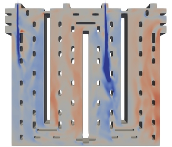
Figure 4.
Turbulent kinematic viscosity on the symmetry plane at s of computation time.

Figure 5.
Inverse of the turbulent time scale (left, logarithmic scale) and combustion energy source term (right, logarithmic scale) on the symmetry plane at s of computation time.
Figure 5.
Inverse of the turbulent time scale (left, logarithmic scale) and combustion energy source term (right, logarithmic scale) on the symmetry plane at s of computation time.

Figure 6.
Temperature (in degrees Celcius) on the symmetry plane (top left), on probe lines through the flame (top right), at the outlet of Burner-1 on the symmetry plane (middle left), at the outlet of Burner-2 on the symmetry plane (middle right), on the plane through Burner-1 perpendicular to the symmetry plane (bottom left) and on the plane through Burner-2 perpendicular to the symmetry plane (bottom right). Values at of computation time are shown.

Figure 7.
Computed equivalence ratio on two probe lines at after of simulation time.

Figure 8.
Mass fraction of CH (left, truncated to 0.1) and O on the symmetry plane (right) at s of computation time.
Figure 8.
Mass fraction of CH (left, truncated to 0.1) and O on the symmetry plane (right) at s of computation time.

Figure 9.
Mass fraction of CO (left) and HO (right) on the symmetry plane at s of computation time.

Figure 10.
Computed thermal absorption coefficient on the symmetry plane after of simulation time.

Figure 11.
Computed mass fraction of OH (left) and thermal NO (right) near Burner-1 (top) and near Burner-2 (bottom) at s of computation time.
Figure 11.
Computed mass fraction of OH (left) and thermal NO (right) near Burner-1 (top) and near Burner-2 (bottom) at s of computation time.


Table 1.
Geometrical and material properties of the thermally insulating lining and boundary conditions imposed.
Table 1.
Geometrical and material properties of the thermally insulating lining and boundary conditions imposed.
| Properties of the Lining | |
|---|---|
| thickness (D) | 0.11 m |
| density () | |
| specific heat capacity () | |
| thermal conductivity (k) | |
| wall emissivity () | |
| outside wall temperature () | |
Table 2.
Inlet conditions for preheated air and natural gas in single section of anode baking furnace.
Table 2.
Inlet conditions for preheated air and natural gas in single section of anode baking furnace.
| Inlet Conditions of Preheated Air | |
|---|---|
| x-Component of velocity () | |
| Temperature (T) | |
| Turbulent kinetic energy (k) | |
| Turbulent dissipation () | |
| Inlet Conditions of Natural Gas at Both Burners | |
| y-Component of velocity () | |
| Temperature (T) | |
| Turbulent kinetic energy (k) | |
| Turbulent dissipation () | |
Table 3.
Smallest edge length of cells in computational mesh in six zones of the computational domain.
Table 3.
Smallest edge length of cells in computational mesh in six zones of the computational domain.
| Zone | Location in the Geometry | Smallest Edge Length |
|---|---|---|
| Zone 1 | Interior of Two Fuel Pipes | 2 mm |
| Zone 2 | Near Walls of Tie Bricks with Curved Corners | 8 mm |
| Zone 3 | Inside of Refinement Zone at Two Fuel Pipe Exits | 16 mm |
| Zone 4 | Near Walls of Tie Bricks with Sharp Corners | 32 mm |
| Zone 5 | Near Walls of Main Channel | 32 mm |
| Zone 6 | Interior of Main Channel | 64 mm |
Publisher’s Note: MDPI stays neutral with regard to jurisdictional claims in published maps and institutional affiliations. |
© 2022 by the authors. Licensee MDPI, Basel, Switzerland. This article is an open access article distributed under the terms and conditions of the Creative Commons Attribution (CC BY) license (https://creativecommons.org/licenses/by/4.0/).
Share and Cite
MDPI and ACS Style
Lahaye, D.; Nakate, P.; Vuik, K.; Juretić, F.; Talice, M. Modeling Conjugate Heat Transfer in an Anode Baking Furnace Using OpenFoam. Fluids 2022, 7, 124. https://0-doi-org.brum.beds.ac.uk/10.3390/fluids7040124
AMA Style
Lahaye D, Nakate P, Vuik K, Juretić F, Talice M. Modeling Conjugate Heat Transfer in an Anode Baking Furnace Using OpenFoam. Fluids. 2022; 7(4):124. https://0-doi-org.brum.beds.ac.uk/10.3390/fluids7040124
Chicago/Turabian StyleLahaye, Domenico, Prajakta Nakate, Kees Vuik, Franjo Juretić, and Marco Talice. 2022. "Modeling Conjugate Heat Transfer in an Anode Baking Furnace Using OpenFoam" Fluids 7, no. 4: 124. https://0-doi-org.brum.beds.ac.uk/10.3390/fluids7040124