
Advances in CFD Modeling of Urban Wind Applied to Aerial Mobility


Aerospace Engineering Area, University of León, Campus dde Vegazana s/n, 24071 León, Spain
*
Author to whom correspondence should be addressed.
Fluids 2022, 7(7), 246; https://0-doi-org.brum.beds.ac.uk/10.3390/fluids7070246
Submission received: 21 June 2022
/
Revised: 12 July 2022
/
Accepted: 15 July 2022
/
Published: 18 July 2022
(This article belongs to the Special Issue Aerodynamics and Aeroacoustics of Vehicles, Volume II)
Abstract
:The feasibility, safety, and efficiency of a drone mission in an urban environment are heavily influenced by atmospheric conditions. However, numerical meteorological models cannot cope with fine-grained grids capturing urban geometries; they are typically tuned for best resolutions ranging from 1 to 10 km. To enable urban air mobility, new now-casting techniques are being developed based on different techniques, such as data assimilation, variational analysis, machine-learning algorithms, and time series analysis. Most of these methods require generating an urban wind field database using CFD codes coupled with the mesoscale models. The quality and accuracy of that database determines the accuracy of the now-casting techniques. This review describes the latest advances in CFD simulations applied to urban wind and the alternatives that exist for the coupling with the mesoscale model. First, the distinct turbulence models are introduced, analyzing their advantages and limitations. Secondly, a study of the meshing is introduced, exploring how it has to be adapted to the characteristics of the urban environment. Then, the several alternatives for the definition of the boundary conditions and the interpolation methods for the initial conditions are described. As a key step, the available order reduction methods applicable to the models are presented, so the size and operability of the wind database can be reduced as much as possible. Finally, the data assimilation techniques and the model validation are presented.

1. Introduction
The use of UAVs in urban areas is becoming a growing trend [1]. This is due to numerous applications varying from civil security to parcel delivery. In spite of this considerable interest, the flight of drones in cities is a genuine challenge due to the high turbulence levels and the drastic changes in wind patterns experienced by the aircraft [2]. This is further aggravated given that the small size of the aircraft increases its vulnerability to weather.
To guarantee the safety of these missions, it is essential to know, as precisely as possible, the wind and turbulence conditions that the aircraft are likely to undergo [3]. Traditionally, mesoscale models have been the tools used to numerically predict the weather [4]. These algorithms implement full-physical models, including long- and shortwave radiation, surface interaction, planetary boundary layer and, of course, water vapor and rain behavior. Nevertheless, these models have best resolutions in the range of 1–1.5 km at best, which is insufficient to accurately represent the relevant scales for the operation of UAVs [5].
CFD simulations are typically used to obtain the required resolution of this application [6]. Usually, the initial and boundary conditions are interpolated from the results produced by a coarser mesoscale prediction, making it necessary to have a proper procedure for the coupling of both models. Though reliable results are obtained, the high cost, both in time and resources, makes this technique unfeasible for real-time now-casting as per today.
Given the previous, current studies are focused on refining the predictions (mainly wind fields) made with mesoscale models using other auxiliary numerical techniques, such as neural networks and sparse regression techniques [7,8], in order to enhance the spatial and temporal resolution. Most of these algorithms, however, require training with huge datasets of real wind fields. In order to generate these wind fields, CFD simulations are again necessary.
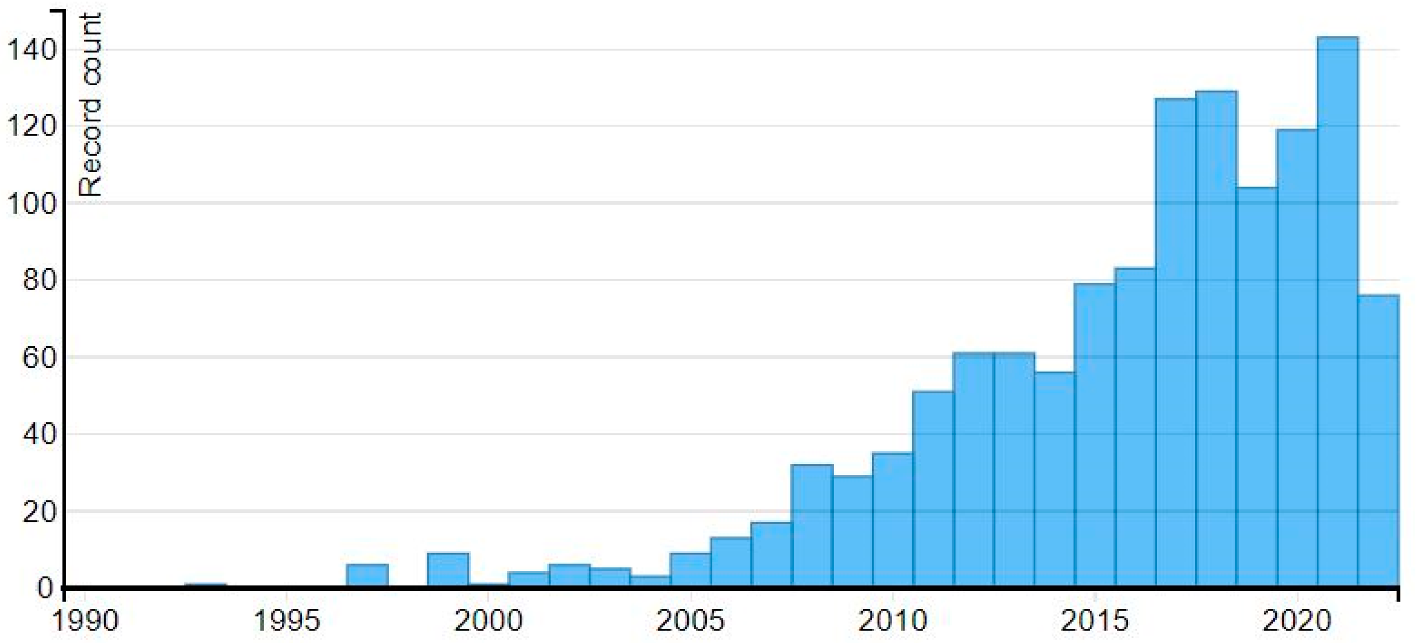
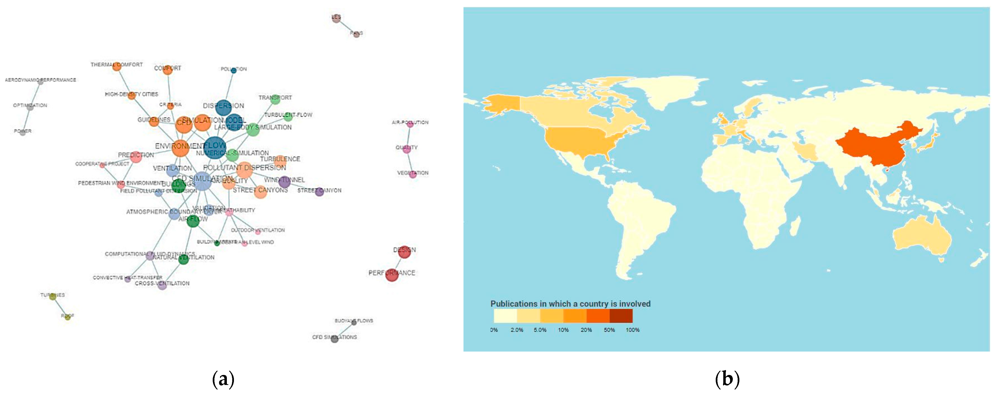
A brief bibliometric analysis was undertaken for this review, along with detailed a continuation. The following databases were analyzed for searching scientific articles: Scopus, Web of Science, and Google Scholar. Web of Science was selected because it generates the largest number of results. The following search criteria (query string) were adopted and applied to the fields for title, keywords, or abstract: “CFD urban winds” or “CFD city wind” or “RANS city wind” or “RANS urban winds”. After filtering, using the tool Biblio ToolBox [9], 1266 scientific papers directly related to the topic were identified in the period from January 1990 to the present. Figure 1 shows the number of publications per year. The total number of publications for each of the five countries with the largest number of papers were China (421), USA (123), UK (114), Italy (83), and Japan (82). The relevance of each country is shown in Figure 2 together with the most relevant keywords that appear in the abstracts.
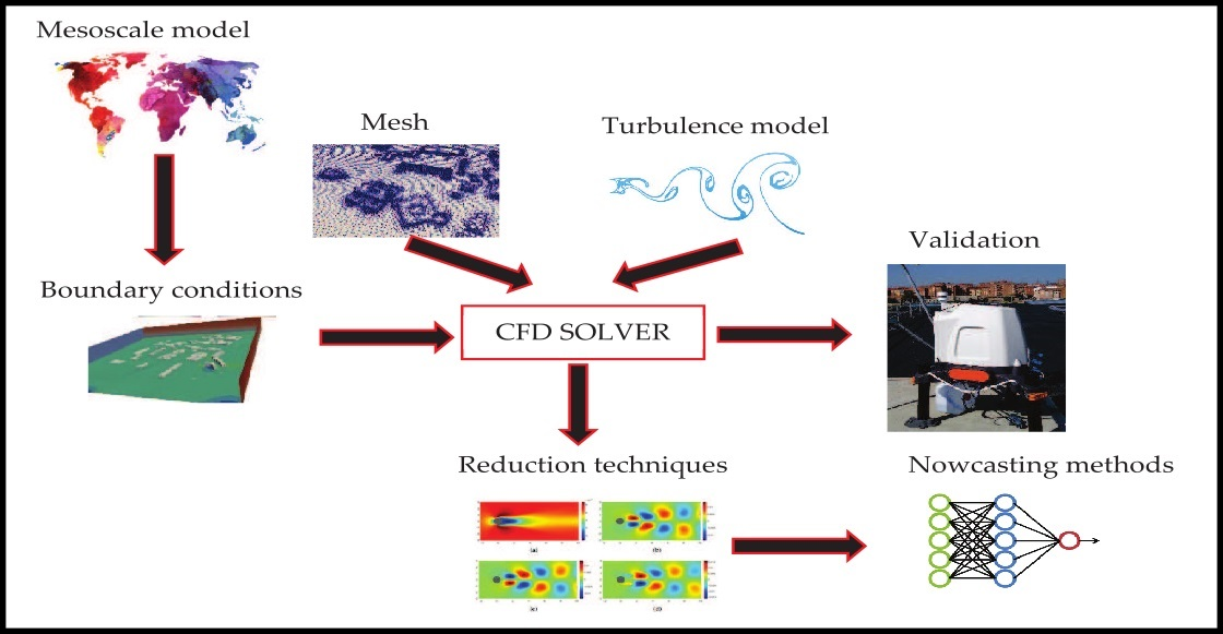
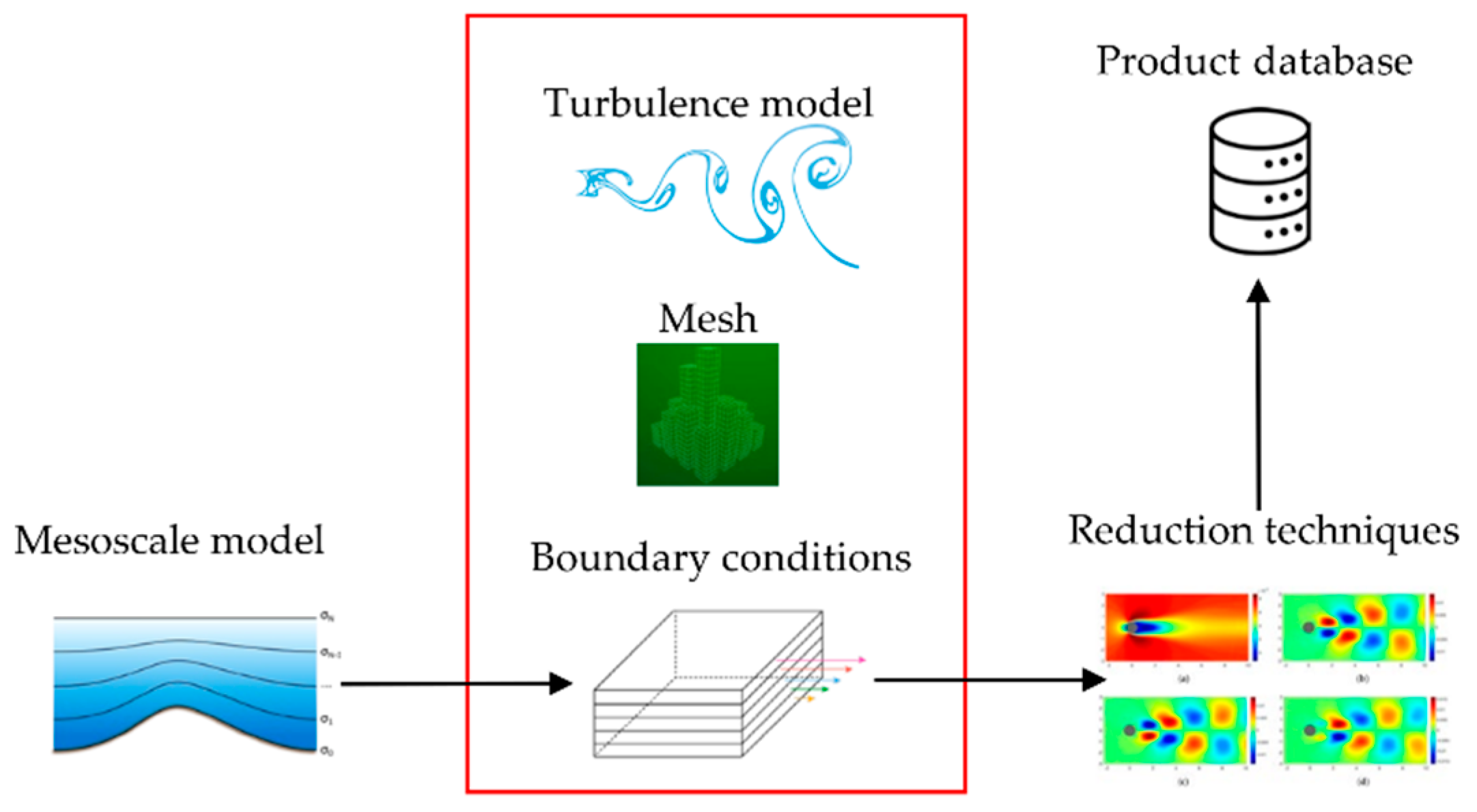
This paper presents the recent advancements in CFD simulation of urban wind to examine how these advancements can be applied to obtain the datasets required to train the now-casting algorithms (see Figure 3). Section 2 describes the different turbulence models available, as well as the modifications to be applied to the closure coefficients. In Section 3, the emphasis is on the preparation of the digital terrain model and the meshing necessary for the simulations. Subsequently, the way that the mesoscale model forecasts have to be interpolated to obtain the initial and boundary conditions of the CFD simulations is discussed. Finally, as the goal was to generate a wind database of a substantial size, different model order reduction techniques are explored. To validate the CFD simulations and increase the reliability of the results, experimental measurements can also be considered, as detailed in Section 5.
2. Turbulence Models
The first question is related to the CFD engine and, more specifically, to which turbulence model is optimal to solve the CFD simulations. In fact, it is possible to directly solve the following Navier-Stokes equations without using any modeling assumptions:
where represents the ith component of the fluid velocity at a point in space and time, represents the static pressure, represents the viscous stresses, and represents the fluid density.
This approach is called direct numerical simulation, or DNS, and requires solving the extensive range of temporal and spatial scales of a turbulent flow from the integral scale up to the Kolmogorov length scale. The mesh resolution and time steps required to correctly resolve the complexity of the fluid structure scale with the 9/4 power of the Reynolds number makes the DNS approach practically unaffordable for engineering applications [10].
The next option is to use LES models. In these models, the smaller scales of the turbulence are spatially filtered:
Meanwhile the larger, more energy-containing scales are solved directly. The symbol denotes the filtering kernel. Given the inherent nature of turbulence, at a very small scale, the flow structures tend to be quite similar to each other, even in different applications [11]. This allows the use of simpler turbulence models for these particular scales.
Finally, in RANS models, the flow is decomposed in two parts: a mean (capital letter) component and a fluctuating component:
This way, the equations for the conservation of momentum can be written as:
where is the averaging operator and the terms are known as the Reynolds stresses. The RANS models are characterized by the fact that the Reynolds stresses are fully modeled.
Turbulence models are typically classified according to the number of additional equations required to model the effect of turbulence on the flow. Models range from simple to complex algebraic relationships and improve their fidelity as the number of equations used increases [12].
It is worth noting that Toparlar et al. [13] investigated 176 studies, reported until 2015, on CFD modeling of urban microclimate, out of which 96% used RANS, 2.8% used LES, and the rest used both. It seems clear, therefore, that there is a predominance for the use of RANS models in this particular application, with an outstanding level of maturity.
As it has been mentioned, DNS is not currently a viable option for these studies, so the decision is between a RANS or a LES model.
LES models are capable of solving the finer scales while modeling the scales in the inertial range. They have been used in several previous works [14], their main drawback being the considerable amount of computational power and time they require. One of the key concerns when simulating urban flows is the large variability and uncertainty of the initial and boundary conditions [15]. Despite using a very accurate turbulence model, which has been successfully validated with experimental results, the errors are not eliminated when comparing predictions against full-scale measurements [16]. This was demonstrated, for example, in simulations of wind flow in the center of various cities [17]. When compared to RANS results, a more expensive and detailed LES did not systematically improve the mean velocity prediction.
Alternatively, RANS models can significantly reduce computing time. A large number of RANS models are available depending on the type of application. The vast majority of the studies carried out to date have used RANS models, with the standard and realizable models standing out [18,19,20,21,22].
The standard model is inefficient when solving complex three-dimensional flows, such as the one arising in urban environments, due to the onset of strong pressure gradients and flow separation [23]. As an alternative, many authors prefer the realizable model [24], which makes some of the closure coefficients become functions of strain rate and rotation rate. In this way, it allows for a consideration of the impact of the flow rate of deformation; thus, it is more flexible.
Other studies have shown that the RNG [25] model presents better results in most cases examined. Another solution is the Reynolds-stress model, although its accuracy is not significantly better than the other models and it presents convergence problems [25].
Previous studies [26,27,28] have shown that standard eddy viscosity closures are not able to fully capture the physics of the atmospheric boundary layer. The underlying cause of this inadequacy is that the wall functions were developed for the boundary layers attached to the wall, assuming equilibrium conditions, i.e., small pressure gradients, local balance between turbulent energy generation and dissipation, and a constant shear stress in the near-wall region. This is far from conditions analogous to those encountered in urban environments. Therefore, it is necessary to modify the coefficients for a realistic coupling between the mesoscale model and the RANS models. New closure coefficients for the model with the proper near-wall treatment for non-neutral and transient simulation have already been tested by Temel and van Beeck [20].
To model the effect of vegetation zones, the most commonly used method is known as the Darcy–Forchheimer (DF) model [29]. In this model, plants are considered to be a momentum sink, which constitutes a simple and robust tool to depict the flow of air through vegetation, regardless of what its morphology is [30]. Two parameters are necessary to model green areas: the Forchheimer drag and the permeability of the vegetation. The permeability parameter is sensitive to variation between species, while Forchheimer drag is not [30]. Thus, the main limitation of these methods is that it depends on the plant morphologies and it should be adapted to the particular situation of study.
Another alternative is to use the model of Shaw and Schumann [31,32], assuming that turbulent kinetic energy is dissipated by the canopy due to the rapid dissipation of wake turbulence in the lee of plant elements. Thus, the plant canopy acts as a sink for momentum due to pressure and viscous drag forces. More details about the model can be found in [31,32]. Several studies apply similar roughness setting methods for the ground surface to approximate building structures [33].
It is worth highlighting several specific implementations of the CFD models:
- MITRAS [34], defined by authors as a “microscale obstacle-resolving model”, computes the wind components, temperature, humidity, and precipitation fields, explicitly resolving obstacles, such as buildings, which are represented by impermeable grid cells at the building positions so that the wind speed vanishes in these grid cells.
- PALM [35], which is an abbreviation for “Parallelized Large-Eddy Simulation Model”, has been widely used to model the atmospheric layer both in the ocean and on land. It uses an LES turbulence model and is especially focused on parallelization. PALM has been used to study ventilation at the pedestrian level, to study wind in street canyons, and even to simulate entire cities. In this regard, the simulation of the city of Macau stands out [36]. The simulation domain has an extension of 30 km2 and a spatial resolution of 1 m. The simulation time was about one hour, while the results required 128 CPUs in parallel, running for 1.5 h.
- ASMUS [37] has been specifically designed to simulate wind and temperature distribution in cities. The turbulence model is RANS and employs the Prandtl–Kolmogorov relation to fulfill the kinetic energy of turbulence modeling. They achieved mesh resolutions of 2 m and were able to simulate more than 44 h. However, the total CPU time is not included in the original paper and it appears that no other studies since 2014 have used this software.
- ENVI-met [38] is built on RANS equations using a 1.5 order turbulence closure model. Some studies [39] mentioned that this closure model tends to overestimate the turbulent production in areas with high acceleration or deceleration, such as the flow around a building. ENVI-met is the detailed vegetation model, in which plants are not only symbolized as a porous media to solar insolation and wind flow, but could actually interact with the surrounding environment by evapotranspiration [40] It has been used to study the wind pattern in cities such as Bilbao [39]. Unlike the other options, it is a paid software.
3. Meshing
Meshing is one of the most important stages of any CFD simulation. In principle, meshing can be achieved with any of the several available software packages (open or paid). Often, the selection of this software depends on the chosen simulation software. Among the various options available, blockMesh/snappyhexMesh (Openfoam) [44], Gambit [45], and ICEM [21] stand out.
One of the most challenging parts of meshing is the generation of the digital terrain model that forms one of the boundaries of the simulation domain. Many studies utilize existing digital terrain models (DTMs) of large or major cities [46]. Other projects with more financial resources create their own maps using LIDAR instruments or satellite products [47]. However, it is currently feasible to build digital models of many cities around the world at almost no cost. The digital models can be built through geographic information system (GIS) data, such as the model given by the AW3D Satellite [48] or European national geographic institutes [49]. These institutes, following the European Directive Inspire (Directive 2007/2/EC, Infrastructure for Spatial Information in Europe), provides web services that allow the download of predefined geographic datasets using ATOM technology [50].
However, with this information, the buildings can be reconstructed in a horizontal plane because the ATOM models do not consider the contribution of the terrain to the difference in the heights of the ground itself and, consequently, the heights of the roofs of the buildings.
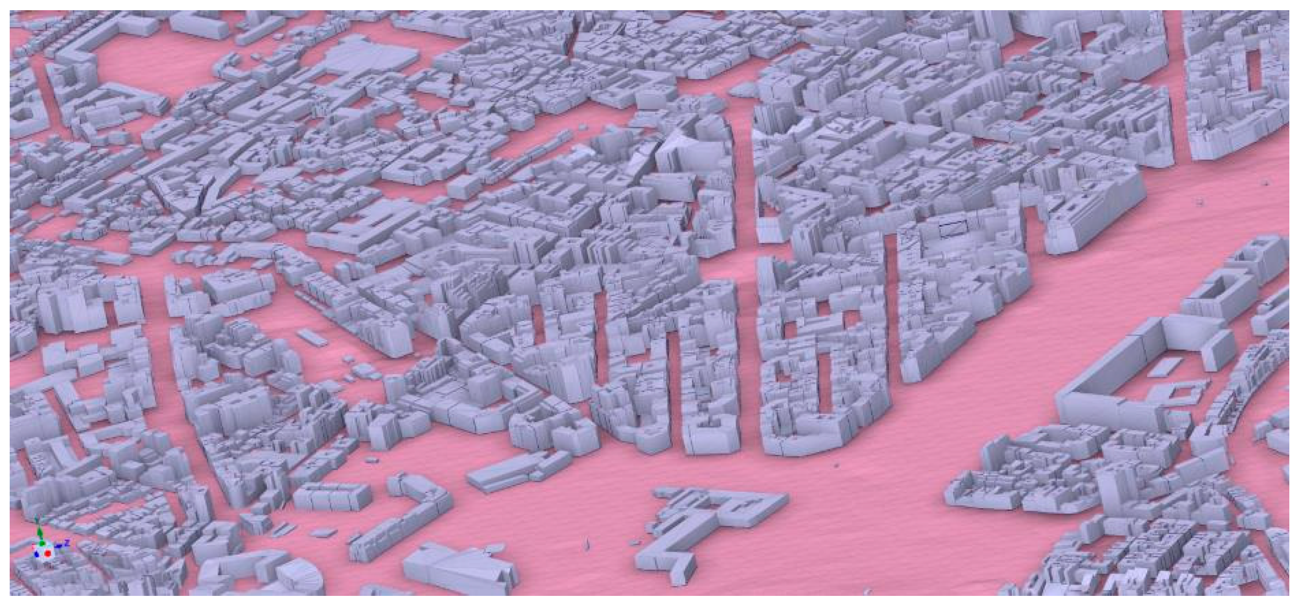
To solve this problem, the data of the city map has to be fused with the geographic properties of the terrain. In many countries, the DTM of the region of interest can be downloaded from the different national centers for geographic information [50]. Joining the data from both sources, a complete model can be obtained. For example, Figure 4 shows how the proposed methodology allows the creation of a 3D model of a medium-sized Spanish city.
Experiments have found that in the simulation of large-scale urban wind fields, low-rise buildings and buildings with too small an area have little impact on the wind field of the whole city [42]. Thus, the urban building models can be simplified to reduce the amount of data and calculations in urban-scale CFD wind field simulations. Li et al. [46] proposed an algorithm to perform this simplification based on ArcGIS 10.2 (ESRI, California, EEUU) to complete the building data generalization program. However, it is unclear how these simplifications could potentially impact the operation of UAVs.
Typically, the vertical extension of the simulation domain is determined by the lockage ratio. That number is defined as the ratio of the projected area of the obstacles to the cross-section of the computational domain, and it is generally required to be less than 3%. Further studies may focus on dynamically adjusting the vertical extent of the domain based on calculations from the mesoscale meteorological models [51].
Due to some instability problems in numerical solutions, in many studies, simulation domains are artificially extended to include fetch zones (typically 10% of the domain length). These regions are added to allow the development of the boundary layer before the flow reaches the modeling region of interest and can be used to avoid pressure field anomalies at the inlet [52].
The use of hexahedral meshes is recommended, since the use of tetrahedral meshes often implies the use of low-order numerical discretization methods. This way, the poor grid quality is compensated with numerical diffusion errors caused by first-order schemes. Although these errors cause a stabilizing effect, the quality of the simulation is reduced [28].
The resolution of the mesh must be sufficient to capture the behavior of the smallest scales. In general, for urban winds, at least a 10 cell per cube root of the building volume is recommended as well as 10 cells in between every two buildings. It should not be forgotten that the overall resolution must be analyzed by means of a mesh convergence study for which at least three different meshes must be used, with a refinement factor of about 1.5 in each direction. This study must be accompanied by an evaluation of errors by what is known as Richardson extrapolation [53].
4. Boundary Conditions
Once the turbulence model has been selected and the meshing process has been successfully completed, it is time to set up the boundary conditions.
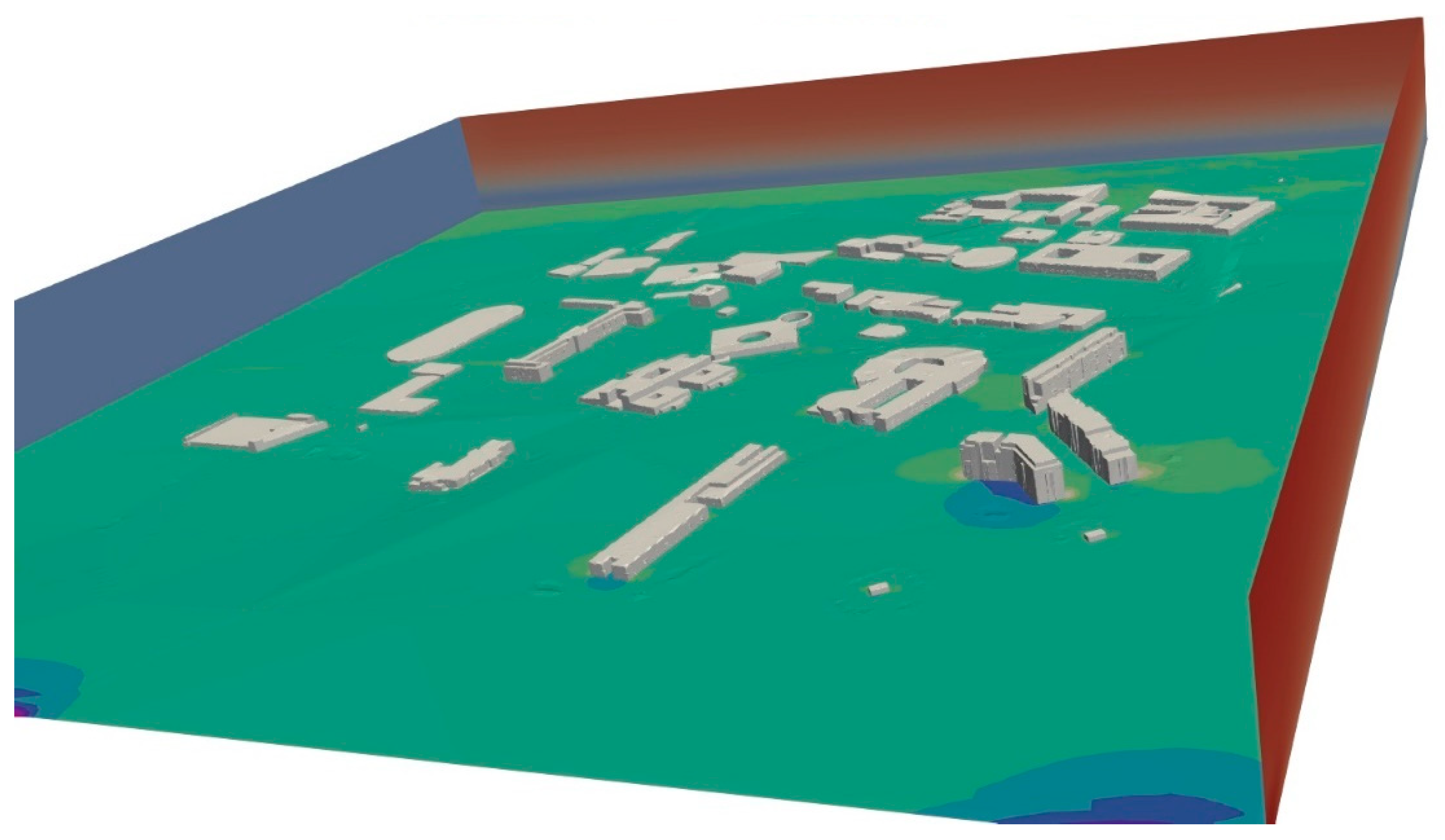
In general, the simulation domain is a prism with six boundary faces (see Figure 5). On the bottom face, the ground, the no-slip condition is set, using the appropriate wall functions for the turbulence model variables. For the remaining five faces, different strategies have been used:
- One of the most common options is known as extrapolation [54]. In this method, only one of the mesoscale model profiles is imposed on an entire inlet face of the CFD domain, while the mesoscale wind data are extrapolated in the grid points outside that profile. This method is the easiest to implement; however, the distributions of the wind velocity on the boundary is uniform in the horizontal direction and, as a consequence, extrapolation is not capable of appropriately coupling the mesoscale and CDF solvers over complex terrains.
- Imposing the zero-gradient boundary conditions at the outflow boundaries and a space-varying inlet condition is another solution [55]. The problem with this solution is in determining which boundary is an inlet and which one is outlet, and how that configuration can change from one day to another.
- The side and top surfaces are modeled as spatially and time-varying velocity inflow and outflow conditions, and the data are extracted from the mesoscale model solutions using interpolation [56]. This solution is the most robust while it comes at the price of implementation complexity.
As it has been seen, in all methods it is required to interpolate the value from the mesoscale mesh to the CFD mesh. Different difficulties can be found when conducting that interpolation. First of all, the horizontal and vertical spacing of each model are very different from each other. In addition, the topography of the boundaries in the CFD domain can also be very different from those of the mesoscale domain. Usually, the interpolation scheme selected is the trilinear interpolation [57]. However, as an alternative, the Cressman interpolation [58] or the inverse distance weighting (IDW) [59] method can be used instead. This way, a great improvement of the models can be achieved [60].
Near the ground (i.e., the first cell of the mesoscale model), all the interpolation schemes may increase the errors, so the velocity is computed following the wall law [61]:
in which is the shear velocity, is the von Kárman constant, is the wind speed, and is the distance from the boundary at which the idealized velocity given by the law of the wall goes to zero. Since the mesh of the CFD model has a higher resolution than that of the mesoscale model, it is possible that the ground does not match in both models. In that case, the mesoscale model profiles are shifted until the origin coincides with the CFD model terrain.
When the atmosphere is non-neutral, the Monin–Obukhov similarity theory should be used instead of Equation (6):
in which the non-neutral condition is modelled by the stability function . is known as the Obukhov length and determines the stability of the atmospheric boundary layer [62]. In a neutral boundary layer, the effects of buoyancy are neglectable, as the temperature of an air parcel decreases at the same rate as that of the surroundings. The neutral condition is the characteristic regime of windy and cloudy conditions so that there is neither a strong heating nor cooling over the surface. The boundary layer tends to be unstable during sunny days when the surface is warmer than the air. Conversely, the atmosphere tends to be stable at night when the surface is cooler than the air.
Apart from the interpolation scheme, it is also important to determine how to compute the variables of the turbulence closure of the CFD, i.e., the kinetic turbulence energy and the viscous dissipation. As it is subsequently shown, TKE values for CFD simulations can be directly obtained from the mesoscale grids if the proper physics model has been selected, which are nearer to the building scale domain. However, certain variables, such as the momentum diffusion coefficient and TKE dissipation rate are estimated using parameterized expressions.
Relative to the turbulent kinetic energy, following the methodology of different studies, such as [63,64,65], it is better to use a boundary layer model for the mesoscale solver which explicitly computes the turbulent kinetic energy. In WRF, there are four different options: MYJ, QNSE, MYNN, and BouLac [66]. However, data from several studies suggest that the MYNN scheme is the best option, offering the lowest root mean square error [63,67].
In order to estimate the viscous dissipation, different approaches can be found in literature:
- Baik, Park, and Kim [64], using the turbulence model RNG , estimated the viscosity dissipation using following the equation:in which is a constant fixed to 0.09, is the turbulent kinetic energy, and is the von Kárman constant.
- Mochida et al. [65] calculated the viscous dissipation based on the length scale of the precedent mesoscale domain. In order to do it, they used the following equation:in which is the ration between the spatial scales and . is the closure constant.
- Another method is considered by Tewari et al. [63]. They used the definition of the viscous dissipation:in which the density is computed from the state equation, is a product of the mesoscale model, and is a constant that is usually fixed to 0.09. However, this method seems to produce too high values of viscous dissipation.
5. Dimensionality Reduction Methods
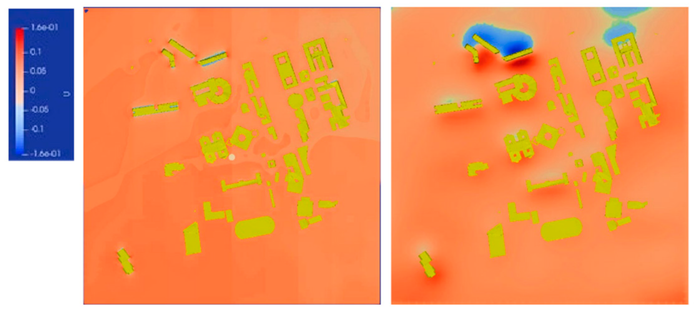
Following the discussion of the introduction, a large number of wind fields are needed to train the numerical now-casting algorithms in such a way that all plausible wind conditions can be collected (see, for example, Figure 6). Due to the considerable size of the files generated in the simulations, it is advisable to use some reduction method in order to minimize the file size. The task is not easy, since the degrees of freedom of the system must be reduced as much as possible while the main characteristics of the system are maintained [68].
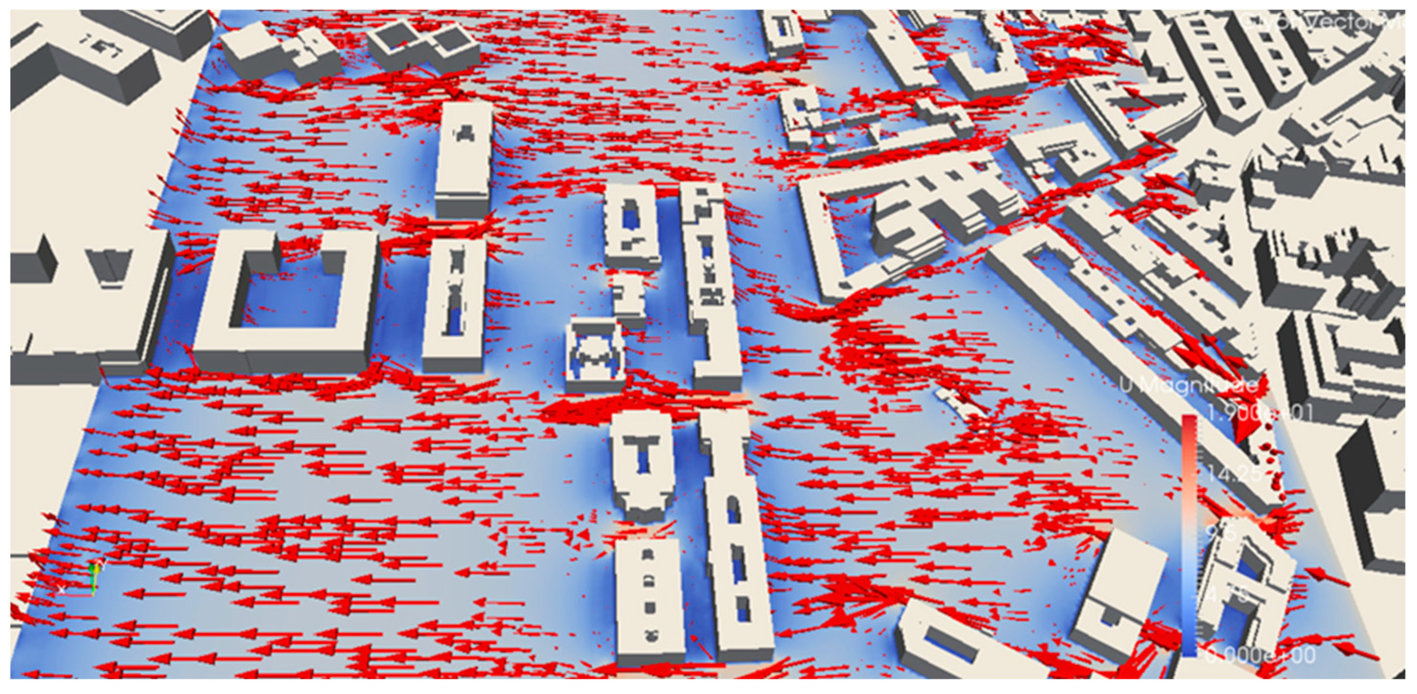
The reduction methods are based on the existence of so-called coherent structures, regions containing the most significant features of the flows [69]. Figure 7, for example, shows how the presence of the buildings causes specific and well-defined wind patterns. By capturing the behavior of these structures, one would be able to reproduce the behavior of the entire wind field with excellent accuracy.
Reduction techniques are classified into two types: linear and nonlinear. An extensive review of both types of methods as applied to urban winds can be found in [70]. Among the linear techniques, the most common is the proper orthogonal decomposition, also known as POD [8,71], in which the most energetic modes in the system can be extracted using the singular value decomposition. To give an idea of its capabilities, Masoumi-Verki et al. [72] reported that, within the wake region of an isolated high-rise building, the contribution of the first 30 POD modes to the total turbulent kinetic energy was about 80.89% and 81.39%, respectively. The total number of wind fields used to calculate the PODs was 4500. Considering that their simulation had approximately 2 million cells, this implies that, instead of storing the 108 Gb of their initial data, they could reconstruct 80% of the kinetic energy using just 1Gb of data. The compression rate improves as the size of the simulations and the number of snapshots increase.
Contrary to the POD, the dynamic mode decomposition computed the modes based on the dynamics of the system rather than the energy content [73]. A POD mode may contain a continuous frequency spectrum, while each DMD mode is characterized by a single frequency. This is a major difference between the two methods, innately. Sometimes, if a flow structure contains relatively small energy but is strongly connected to other structures sharing the same frequency, this structure is likely to be ignored by POD analysis but would be captured by the DMD. However, up to this day, PODs are still the most widely used linear technique [74,75,76,77,78].
Of course, the major drawback of both the POD and the DMD is their linear nature. They project the wind field snapshots in an optimal linear subspace. However, the non-linear nature of the Navier-Stokes equations and the dynamic boundary conditions [79,80] can penalize the performance of these algorithms. It is for these reasons that many authors argue that using linear dimensionality reduction techniques is not the most suitable choice for urban wind now-casting [70].
This hypothesis has been supported by several studies comparing POD techniques with nonlinear methods based on encoders [80]. The nonlinear approaches performed better in obtaining a low-dimensional model of the original data. Other investigations based on nonlinear reduction may be found in [79,80,81]. At the present time, research is also being conducted on deep learning methods [82] with promising results.
6. Data Assimilation and Validation
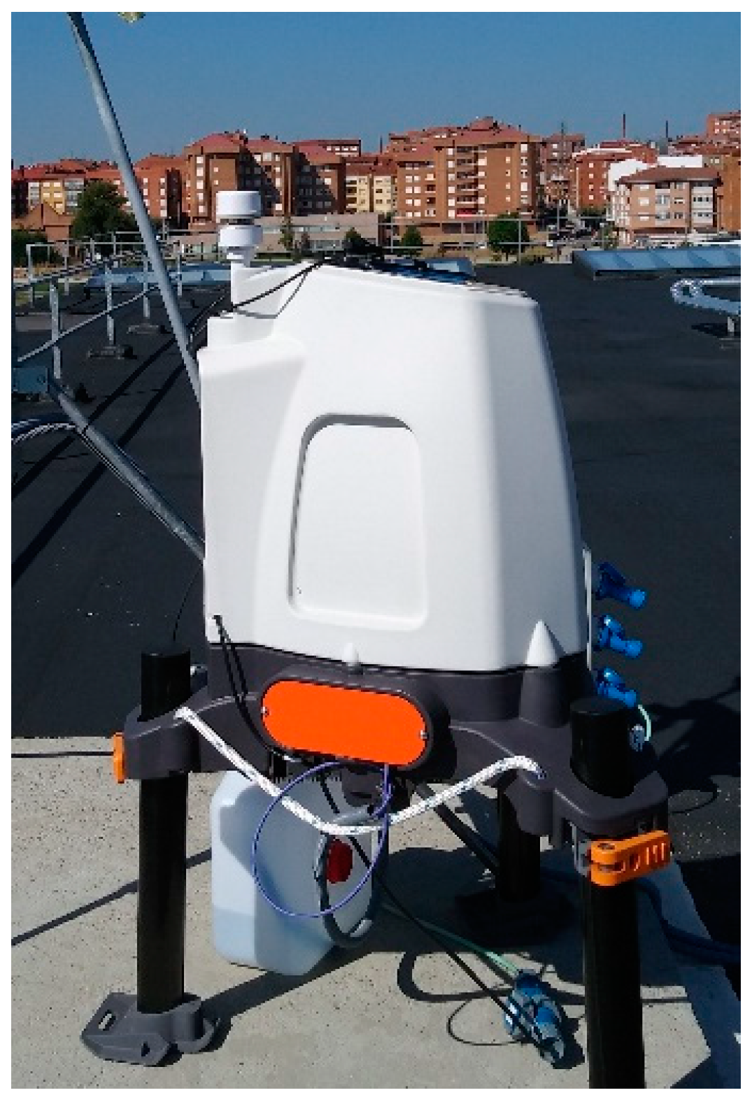
Finally, to check the performance and to improve the reliability of the CFD simulations, it is necessary to validate the results. This can be done using wind tunnel experiments [83]. This approach faces the challenge of actually being able to produce realistic wind conditions, in spite of the cost of building the test models and of the wind tunnel operation. The second option is to deploy multiple wind sensors throughout the city under study and to compare the measurements recorded by the instruments to the results of the simulations for specific wind conditions. As sensors, one may find a wide range of solutions from meteorological stations [84] to LIDAR instruments [61,85], such as in Figure 8, satellites [86], and/or other more innovative methods [87].
Despite all previous efforts, it is unlikely that the predictions made are completely accurate, i.e., they must be adjusted according to the measurements made by a network of sensors distributed throughout the city. In this manner, data assimilation using wind sensors located within the urban canopy offers promising possibilities to enhance the reliability of the predictions.
Considerable studies have discussed how to accomplish this data assimilation. The different algorithms rely mainly on either variational principles [88], nonlinear Kalman filters [89], and/or Bayesian techniques [90].
Under that premise, there are currently several ongoing studies that have addressed the use of real wind measurements from UAVs to solve the inverse problem of predicting wind conditions as it flies over the city [91]. The most common method to do it is the use of a particle filter in combination with a surrogate model [92,93].
Although the results are encouraging, it should be noted that, due to the large size of cities and the high variability of winds around buildings, the number of sensors required is expected to be relatively high. For this reason, and also due to the cost of acquisition and maintenance of wind sensors, it is essential to optimize their distribution. This optimization has been studied in several studies, such as [94,95].
7. Conclusions
Currently, the implementation of U-space in urban environments requires now-casting techniques that can accurately estimate wind fields and turbulence levels. Since the resolution of mesoscale models is not sufficient and CFD models require too much simulation time, the most suitable solution is to use a machine-learning algorithm trained with a large dataset of wind field data. In this review, we have collected the key steps for the elaboration of this database: choice of the turbulence model, creation of the mesh, interpolation of the boundary conditions from the mesoscale fields, and the necessary order reduction methods.
Due to the high number of wind field required to train the prediction algorithms, the use of RANS-type turbulence models is preferable. The models are currently a standard for this type of study, although it is necessary to modify the closure turbulence.
Concerning the meshing, obtaining the digital model of the terrain and the buildings is one of the most difficult steps. Other recommendations are: to use hexahedral cells to reduce numerical diffusion, to adequately refine the high gradient zones, and to perform the corresponding sensitivity analysis of the mesh.
The initial and boundary conditions are to be interpolated from the mesoscale model results. The Cressman interpolation is outstanding for this purpose, except for the cells closest to the ground, where the logarithmic law must be considered. For determining the viscous dissipation, there are several alternatives, which have been described in this document.
In the post-processing phase, the result is to reduce the size of the wind fields as much as possible while preserving their most relevant characteristics. With more conventional techniques, such as POD or DMD, compression ratios of up to 100 can be achieved. This rate can be increased even further by means of nonlinear methods, the study of which is currently on the rise.
Finally, it is important to highlight the relevance of making these databases publicly accessible. In this way, the different now-casting algorithms could be tested, trained, and validated using the same data, encouraging their continuous evolution.
Author Contributions
Conceptualization, A.G.-G. and J.G.; methodology, D.L. and A.G.-G.; formal analysis, J.G. and A.D.; investigation, A.G.-G. and D.L.; resources, J.G.; writing—original draft preparation, A.G.-G. and A.D.; writing—review and editing, J.G. and D.L.; visualization, D.L.; supervision, J.G.; project administration, J.G. All authors have read and agreed to the published version of the manuscript.
Funding
This research received no external funding.
Data Availability Statement
Not applicable.
Acknowledgments
The authors acknowledge the valuable suggestions of the anonymous referees that helped to enhance the manuscript.
Conflicts of Interest
The authors declare no conflict of interest.
Nomenclature
| Closure constant | |
| Mathematical constant | |
| DF | Darcy–Forchheimer model |
| DNS | Direct numerical simulation |
| DMD | Dynamic mode decomposition |
| DTM | Digital terrain model |
| IDW | Inverse distance weighting interpolation |
| G | Filtering kernel |
| GIS | Geographic information system |
| Turbulence kinetic energy | |
| LES | Large-eddy simulation |
| Static pressure | |
| P | Mean component of the pressure |
| POD | Proper orthogonal decomposition |
| p | Fluctuating component of the pressure |
| RANS | Reynolds-averaged Navier–Stokes equations |
| UAV | Unmanned aerial vehicle |
| i-the component of the fluid velocity | |
| Mean component of the velocity | |
| Fluctuating component of the velocity | |
| Shear velocity | |
| Viscous stresses | |
| Turbulence dissipation | |
| von Kárman constant | |
| fluid density | |
| Specific rate of dissipation of turbulence kinetic energy |
References
- Barrado, C.; Boyero, M.; Brucculeri, L.; Ferrara, G.; Hately, A.; Hullah, P.; Martin-Marrero, D.; Pastor, E.; Rushton, A.P.; Volkert, A. U-Space Concept of Operations: A Key Enabler for Opening Airspace to Emerging Low-Altitude Operations. Aerospace 2020, 7, 24. [Google Scholar] [CrossRef] [Green Version]
- Lieb, J.; Volkert, A. Unmanned Aircraft Systems Traffic Management: A comparison on the FAA UTM and the European CORUS ConOps based on U-space. In Proceedings of the 2020 AIAA/IEEE 39th Digital Avionics Systems Conference (DASC), San Antonio, TX, USA, 11 October 2020; pp. 1–6. [Google Scholar] [CrossRef]
- Sunil, E.; Sun, J.; Koerse, R.; van Selling, S.; van Doorn, J.-W.; Brinkman, T. METSIS: Hyperlocal Wind Nowcasting for U-space Knowledge extraction from large-scale air traffic data View project METSIS: Hyperlocal Wind Nowcasting for U-space. In Proceedings of the 11th SESAR Innovation Days, Virtual Event, 7 December 2021; pp. 1–8. [Google Scholar]
- Gonzalo, J.; Domínguez, D.; López, D.; García-Gutiérrez, A. An analysis and enhanced proposal of atmospheric boundary layer wind modelling techniques for automation of air traffic management. Chin. J. Aeronaut. 2021, 34, 129–144. [Google Scholar] [CrossRef]
- Kadaverugu, R.; Sharma, A.; Matli, C.; Biniwale, R. High Resolution Urban Air Quality Modeling by Coupling CFD and Mesoscale Models: A Review. Asia-Pac. J. Atmos. Sci. 2019, 55, 539–556. [Google Scholar] [CrossRef]
- Grushin, A.; Tyagi, A.; Gluck, J.; Mohseni, S.; Nigam, N.; Klopfenstein, M.; Lee, R.S. Gump: General urban area microclimate predictions tool. In Proceedings of the AIAA AVIATION 2020 FORUM, Virtual Event, 15–19 June 2020; pp. 1–17. [Google Scholar] [CrossRef]
- Sofos, F.; Stavrogiannis, C.; Exarchou-Kouveli, K.K.; Akabua, D.; Charilas, G.; Karakasidis, T.E. Current Trends in Fluid Research in the Era of Artificial Intelligence: A Review. Fluids 2022, 7, 116. [Google Scholar] [CrossRef]
- Vuppala, R.K.S.S.; Kara, K. A Novel Approach in Realistic Wind Data Generation for the Safe Operation of Small Unmanned Aerial Systems in Urban Environment. In Proceedings of the AIAA AVIATION 2021 FORUM, Virtual Event, 2–6 August 2021. [Google Scholar] [CrossRef]
- Grauwin, S.; Jensen, P. Mapping scientific institutions. Scientometrics 2011, 89, 943–954. [Google Scholar] [CrossRef] [Green Version]
- Karniadakis, G.E.; Orszag, S.A. Nodes, Modes and Flow Codes. Phys. Today 2008, 46, 34. [Google Scholar] [CrossRef] [Green Version]
- Mansouri, Z.; Verma, S.; Selvam, R.P. Teaching Modeling Turbulent Flow around Building Using LES Turbulence Method and Open-source Software OpenFOAM. In Proceedings of the 2021 ASEE Midwest Section Conference, Virtual Event, 17 November 2021. [Google Scholar] [CrossRef]
- Heinz, S. A review of hybrid RANS-LES methods for turbulent flows: Concepts and applications. Prog. Aerosp. Sci. 2020, 114, 100597. [Google Scholar] [CrossRef]
- Toparlar, Y.; Blocken, B.; Maiheu, B.; van Heijst, G. A review on the CFD analysis of urban microclimate. Renew. Sustain. Energy Rev. 2017, 80, 1613–1640. [Google Scholar] [CrossRef]
- García-Sánchez, C.; van Beeck, J.; Gorlé, C. Predictive large eddy simulations for urban flows: Challenges and opportunities. Build. Environ. 2018, 139, 146–156. [Google Scholar] [CrossRef]
- Schatzmann, M.; Leitl, B. Issues with validation of urban flow and dispersion CFD models. J. Wind Eng. Ind. Aerodyn. 2011, 99, 169–186. [Google Scholar] [CrossRef]
- Blocken, B. LES over RANS in building simulation for outdoor and indoor applications: A foregone conclusion? Build. Simul. 2018, 11, 821–870. [Google Scholar] [CrossRef] [Green Version]
- Gorlé, C. Improving Predictions of the Urban Wind Environment Using Data. Technol. Archit. Des. 2019, 3, 137–141. [Google Scholar] [CrossRef]
- Ricci, A.; Kalkman, I.; Blocken, B.; Burlando, M.; Repetto, M.P. Impact of turbulence models and roughness height in 3D steady RANS simulations of wind flow in an urban environment. Build. Environ. 2020, 171, 106617. [Google Scholar] [CrossRef]
- Zheng, X.; Montazeri, H.; Blocken, B. CFD simulations of wind flow and mean surface pressure for buildings with balconies: Comparison of RANS and LES. Build. Environ. 2020, 173, 106747. [Google Scholar] [CrossRef]
- Temel, O.; Porchetta, S.; Bricteux, L.; van Beeck, J. RANS closures for non-neutral microscale CFD simulations sustained with inflow conditions acquired from mesoscale simulations. Appl. Math. Model. 2018, 53, 635–652. [Google Scholar] [CrossRef] [Green Version]
- Shirzadi, M.; Tominaga, Y.; Mirzaei, P.A. Experimental and steady-RANS CFD modelling of cross-ventilation in moderately-dense urban areas. Sustain. Cities Soc. 2020, 52, 101849. [Google Scholar] [CrossRef]
- Temel, O.; van Beeck, J. Adaptation of mesoscale turbulence parameterisation schemes as RANS closures for ABL simulations. J. Turbul. 2016, 17, 966–997. [Google Scholar] [CrossRef]
- Longo, R.; Ferrarotti, M.; Sánchez, C.G.; Derudi, M.; Parente, A. Advanced turbulence models and boundary conditions for flows around different configurations of ground-mounted buildings. J. Wind Eng. Ind. Aerodyn. 2017, 167, 160–182. [Google Scholar] [CrossRef] [Green Version]
- Jian, Z.; Bo, L.; Mingyue, W. Study on windbreak performance of tree canopy by numerical simulation method. J. Comput. Multiph. Flows 2018, 10, 259–265. [Google Scholar] [CrossRef]
- Koutsourakis, N.; Bartzis, J.G.; Markatos, N.C. Evaluation of Reynolds stress, k-ε and RNG k-ε turbulence models in street canyon flows using various experimental datasets. Environ. Fluid Mech. 2012, 12, 379–403. [Google Scholar] [CrossRef]
- Zhao, Z.; Xiao, Y.; Li, C.; Wang, J.; Hu, G. New consideration of lateral boundary treatment for meso- and micro-scale nested PBL simulations over complex terrain. Atmos. Res. 2021, 105507, 1–18. [Google Scholar] [CrossRef]
- Antoniou, N.; Montazeri, H.; Neophytou, M.; Blocken, B. CFD simulation of urban microclimate: Validation using high-resolution field measurements. Sci. Total Environ. 2019, 695, 133743. [Google Scholar] [CrossRef] [PubMed]
- Blocken, B. Computational Fluid Dynamics for urban physics: Importance, scales, possibilities, limitations and ten tips and tricks towards accurate and reliable simulations. Build. Environ. 2015, 91, 219–245. [Google Scholar] [CrossRef] [Green Version]
- Verbruggen, S.W.; Keulemans, M.; van Walsem, J.; Tytgat, T.; Lenaerts, S.; Denys, S. CFD modeling of transient adsorption/desorption behavior in a gas phase photocatalytic fiber reactor. Chem. Eng. J. 2016, 292, 42–50. [Google Scholar] [CrossRef]
- Koch, K.; Samson, R.; Denys, S. Aerodynamic characterisation of green wall vegetation based on plant morphology: An experimental and computational fluid dynamics approach. Biosyst. Eng. 2019, 178, 34–51. [Google Scholar] [CrossRef]
- Cassiani, M.; Katul, G.G.; Albertson, J.D. The Effects of Canopy Leaf Area Index on Airflow across Forest Edges: Large-eddy Simulation and Analytical Results. Bound.-Layer Meteorol. 2007, 126, 433–460. [Google Scholar] [CrossRef] [Green Version]
- Serra-Neto, E.M.; Martins, H.S.; Dias-Júnior, C.Q.; Santana, R.A.; Brondani, D.V.; Manzi, A.O.; de Araújo, A.C.; Teixeira, P.R.; Sörgel, M.; Mortarini, L. Simulation of the Scalar Transport above and within the Amazon Forest Canopy. Atmosphere 2021, 12, 1631. [Google Scholar] [CrossRef]
- Liu, S.; Pan, W.; Zhang, H.; Cheng, X.; Long, Z.; Chen, Q. CFD simulations of wind distribution in an urban community with a full-scale geometrical model. Build. Environ. 2017, 117, 11–23. [Google Scholar] [CrossRef]
- Salim, M.H.; Heinke Schlünzen, K.; Grawe, D.; Boettcher, M.; Gierisch, A.M.U.; Fock, B.H. The Microscale Obstacle Resolving Meteorological Model MITRAS: Model Theory. Geosci. Model Dev. 2018, 11, 3427–3445. [Google Scholar] [CrossRef] [Green Version]
- Gronemeier, T.; Surm, K.; Harms, F.; Leitl, B.; Maronga, B.; Raasch, S. Evaluation of the dynamic core of the PALM model system 6.0 in a neutrally stratified urban environment: Comparison between les and wind-tunnel experiments. Geosci. Model Dev. 2021, 14, 3317–3333. [Google Scholar] [CrossRef]
- Urban Large-Eddy Simulation. Available online: https://av.tib.eu/media/14368 (accessed on 17 July 2022).
- Gross, G. Effects of different vegetation on temperature in an urban building environment. Micro-scale numerical experiments. Meteorol. Z. 2012, 21, 399–412. [Google Scholar] [CrossRef]
- Müller, N.; Kuttler, W.; Barlag, A.B. Counteracting urban climate change: Adaptation measures and their effect on thermal comfort. Theor. Appl. Climatol. 2014, 115, 243–257. [Google Scholar] [CrossRef] [Green Version]
- Acero, J.A.; Arrizabalaga, J. Evaluating the performance of ENVI-met model in diurnal cycles for different meteorological conditions. Theor. Appl. Climatol. 2018, 131, 455–469. [Google Scholar] [CrossRef]
- Liu, Z.; Cheng, W.; Jim, C.Y.; Morakinyo, T.E.; Shi, Y.; Ng, E. Heat mitigation benefits of urban green and blue infrastructures: A systematic review of modeling techniques, validation and scenario simulation in ENVI-met V4. Build. Environ. 2021, 200, 107939. [Google Scholar] [CrossRef]
- Eichhorn, J.; Kniffka, A. The numerical flow model MISKAM: State of development and evaluation of the basic version. Meteorol. Z. 2010, 19, 81–90. [Google Scholar] [CrossRef]
- Farkas, O.; Török, Á. Dust deposition, microscale flow-and dispersion model of particulate matter, examples from the city center of Budapest. J. Hung. Meteorol. Serv. 2019, 123, 39–55. [Google Scholar] [CrossRef] [Green Version]
- Bächler, P.; Müller, T.K.; Warth, T.; Yildiz, T.; Dittler, A. Impact of ambient air filters on PM concentration levels at an urban traffic hotspot (Stuttgart, Am Neckartor). Atmospheric Pollut. Res. 2021, 12, 101059. [Google Scholar] [CrossRef]
- Elfverson, D.; Lejon, C. Use and Scalability of OpenFOAM for Wind Fields and Pollution Dispersion with Building- and Ground-Resolving Topography. Atmosphere 2021, 12, 1124. [Google Scholar] [CrossRef]
- Gallagher, J.; Gill, L.W.; McNabola, A. Numerical modelling of the passive control of air pollution in asymmetrical urban street canyons using refined mesh discretization schemes. Build. Environ. 2012, 56, 232–240. [Google Scholar] [CrossRef]
- Li, M.; Qiu, X.; Shen, J.; Xu, J.; Feng, B.; He, Y.; Shi, G.; Zhu, X. CFD Simulation of the Wind Field in Jinjiang City Using a Building Data Generalization Method. Atmosphere 2019, 10, 326. [Google Scholar] [CrossRef] [Green Version]
- Saeedrashed, Y.S.; Benim, A.C. Validation Methods of Geometric 3D-CityGML Data for Urban Wind Simulations. E3S Web Conf. 2019, 128, 10006. [Google Scholar] [CrossRef]
- Girindran, R.; Boyd, D.S.; Rosser, J.; Vijayan, D.; Long, G.; Robinson, D. On the Reliable Generation of 3D City Models from Open Data. Urban Sci. 2020, 4, 47. [Google Scholar] [CrossRef]
- Atazadeh, B.; Halalkhor Mirkalaei, L.; Olfat, H.; Rajabifard, A.; Shojaei, D. Integration of cadastral survey data into building information models. Geo-Spat. Inf. Sci. 2021, 24, 387–402. [Google Scholar] [CrossRef]
- Technical Guidance for the Implementation of INSPIRE Download Services|INSPIRE. Available online: https://inspire.ec.europa.eu/documents/technical-guidance-implementation-inspire-download-services (accessed on 13 June 2022).
- Kadaverugu, R.; Purohit, V.; Matli, C.; Biniwale, R. Improving accuracy in simulation of urban wind flows by dynamic downscaling WRF with OpenFOAM. Urban Clim. 2021, 38. [Google Scholar] [CrossRef]
- Zajaczkowski, F.J.; Haupt, S.E.; Schmehl, K.J. A preliminary study of assimilating numerical weather prediction data into computational fluid dynamics models for wind prediction. J. Wind Eng. Ind. Aerodyn. 2011, 99, 320–329. [Google Scholar] [CrossRef]
- Franke, J.; Hellsten, A.; Schlünzen, K.H.; Carissimo, B. The COST 732 Best Practice Guideline for CFD simulation of flows in the urban environment: A summary. Int. J. Environ. Pollut. 2011, 44, 419–427. [Google Scholar] [CrossRef]
- Laporte, L.; Dupont, É.; Carissimo, B.; Musson-Genon, L.; Sécolier, C. Atmospheric CFD simulations coupled to mesoscale analyses for wind resource assessment in complex terrain. In Proceedings of the European Wind Energy Conference, Marseille, France, 15–17 March 2009. [Google Scholar]
- A Pre-Processing Utility for Coupling WRF and Openfoam. Available online: https://scholar.googleusercontent.com/scholar?q=cache:dqmW-oxctV8J:scholar.google.com/&hl=en&as_sdt=0,5 (accessed on 31 March 2022).
- Li, S.; Sun, X.; Zhang, S.; Zhao, S.; Zhang, R. A Study on Microscale Wind Simulations with a Coupled WRF–CFD Model in the Chongli Mountain Region of Hebei Province, China. Atmosphere 2019, 10, 731. [Google Scholar] [CrossRef] [Green Version]
- Lundquist, K.A.; Chow, F.K.; Lundquist, J.K. An Immersed Boundary Method Enabling Large-Eddy Simulations of Flow over Complex Terrain in the WRF Model. Month. Weather Rev. 2012, 140, 3936–3955. [Google Scholar] [CrossRef]
- Li, S.; Sun, X.; Zhang, R.; Zhang, C. A Feasibility Study of Simulating the Micro-Scale Wind Field for Wind Energy Applications by NWP/CFD Model with Improved Coupling Method and Data Assimilation. Energies 2019, 12, 2549. [Google Scholar] [CrossRef] [Green Version]
- Wiersema, D.J.; Lundquist, K.A.; Chow, F.K. Mesoscale to Microscale Simulations over Complex Terrain with the Immersed Boundary Method in the Weather Research and Forecasting Model. Month. Weather Rev. 2020, 148, 577–595. [Google Scholar] [CrossRef]
- Zhao, Z.; Li, C.; Xiao, Y.; Wang, J.; Hu, G.; Xiao, K. Multiscale modelling of planetary boundary layer flow over complex terrain: Implementation under near-neutral conditions. Environ. Fluid Mech. 2021, 21, 759–790. [Google Scholar] [CrossRef]
- García-Gutiérrez, A.; Domínguez, D.; López, D.; Gonzalo, J. Atmospheric Boundary Layer Wind Profile Estimation Using Neural Networks Applied to Lidar Measurements. Sensors 2021, 21, 3659. [Google Scholar] [CrossRef] [PubMed]
- Probst, O.; Cárdenas, D. State of the Art and Trends in Wind Resource Assessment. Energies 2010, 3, 1087–1141. [Google Scholar] [CrossRef] [Green Version]
- Tewari, M.; Kusaka, H.; Chen, F.; Coirier, W.J.; Kim, S.; Wyszogrodzki, A.A.; Warner, T.T. Impact of coupling a microscale computational fluid dynamics model with a mesoscale model on urban scale contaminant transport and dispersion. Atmospheric Res. 2010, 96, 656–664. [Google Scholar] [CrossRef]
- Baik, J.J.; Park, S.B.; Kim, J.J. Urban Flow and Dispersion Simulation Using a CFD Model Coupled to a Mesoscale Model. J. Appl. Meteorol. Clim. 2009, 48, 1667–1681. [Google Scholar] [CrossRef]
- Mochida, A.; Iizuka, S.; Tominaga, Y.; Lun, I.Y.F. Up-scaling CWE models to include mesoscale meteorological influences. J. Wind Eng. Ind. Aerodyn. 2011, 99, 187–198. [Google Scholar] [CrossRef]
- Rajeswari, J.R.; Srinivas, C.V.; Mohan, P.R.; Venkatraman, B. Impact of Boundary Layer Physics on Tropical Cyclone Simulations in the Bay of Bengal Using the WRF Model. Pure Appl. Geophys. 2020, 177, 5523–5550. [Google Scholar] [CrossRef]
- Giannakopoulou, E.M.; Nhili, R. WRF model methodology for offshore wind energy applications. Adv. Meteorol. 2014, 2014, 1–14. [Google Scholar] [CrossRef] [Green Version]
- Schmid, P.J.; Garciá-Gutierrez, A.; Jiménez, J. Description and detection of burst events in turbulent flows. J. Phys. Conf. Ser. 2018, 1001, 012015. [Google Scholar] [CrossRef]
- Oehler, S.; Garcia–Gutiérrez, A.; Illingworth, S. Linear estimation of coherent structures in wall-bounded turbulence at Reτ = 2000. J. Phys. Conf. Ser. 2018, 1001, 012006. [Google Scholar] [CrossRef] [Green Version]
- Masoumi-Verki, S.; Haghighat, F.; Eicker, U. A review of advances towards efficient reduced-order models (ROM) for predicting urban airflow and pollutant dispersion. Build. Environ. 2022, 216, 1–13. [Google Scholar] [CrossRef]
- Ding, S.; Yang, R. Reduced-order modelling of urban wind environment and gaseous pollutants dispersion in an urban-scale street canyon. J. Saf. Sci. Resil. 2021, 2, 238–245. [Google Scholar] [CrossRef]
- Masoumi-Verki, S.; Gholamalipour, P.; Haghighat, F.; Eicker, U. Embedded LES of thermal stratification effects on the airflow and concentration fields around an isolated high-rise building: Spectral and POD analyses. Build. Environ. 2021, 206, 108388. [Google Scholar] [CrossRef]
- Wu, Z.; Laurence, D.; Utyuzhnikov, S.; Afgan, I. Proper orthogonal decomposition and dynamic mode decomposition of jet in channel crossflow. Nucl. Eng. Des. 2019, 344, 54–68. [Google Scholar] [CrossRef]
- Quilodrán-Casas, C.; Arcucci, R.; Pain, C.; Guo, Y. Adversarially Trained LSTMs on Reduced Order Models of Urban Air Pollution Simulations. arXiv 2021, preprint. arXiv:2101.01568. [Google Scholar] [CrossRef]
- Quilodrán-Casas, C.; Arcucci, R.; Mottet, L.; Guo, Y.; Pain, C.C. Adversarial Autoencoders and Adversarial LSTM for Improved Forecasts of Urban Air Pollution Simulations. arXiv 2021, preprint. arXiv:2104.06297. [Google Scholar] [CrossRef]
- Xiao, D.; Fang, F.; Heaney, C.E.; Navon, I.M.; Pain, C.C. A domain decomposition method for the non-intrusive reduced order modelling of fluid flow. Comput. Methods Appl. Mech. Eng. 2019, 354, 307–330. [Google Scholar] [CrossRef]
- Xiao, D.; Heaney, C.E.; Fang, F.; Mottet, L.; Hu, R.; Bistrian, D.A.; Aristodemou, E.; Navon, I.M.; Pain, C.C. A domain decomposition non-intrusive reduced order model for turbulent flows. Comput. Fluids 2019, 182, 15–27. [Google Scholar] [CrossRef] [Green Version]
- Xiao, D.; Heaney, C.E.; Mottet, L.; Fang, F.; Lin, W.; Navon, I.M.; Guo, Y.; Matar, O.K.; Robins, A.G.; Pain, C.C. A reduced order model for turbulent flows in the urban environment using machine learning. Build. Environ. 2019, 148, 323–337. [Google Scholar] [CrossRef] [Green Version]
- Xiang, S.; Zhou, J.; Fu, X.; Zheng, L.; Wang, Y.; Zhang, Y.; Yi, K.; Liu, J.; Ma, J.; Tao, S. Fast simulation of high resolution urban wind fields at city scale. Urban Clim. 2021, 39, 100941. [Google Scholar] [CrossRef]
- Xiang, S.; Fu, X.; Zhou, J.; Wang, Y.; Zhang, Y.; Hu, X.; Xu, J.; Liu, H.; Liu, J.; Ma, J.; et al. Non-intrusive reduced order model of urban airflow with dynamic boundary conditions. Build. Environ. 2021, 187, 107397. [Google Scholar] [CrossRef]
- Na, J.; Jeon, K.; Lee, W.B. Toxic gas release modeling for real-time analysis using variational autoencoder with convolutional neural networks. Chem. Eng. Sci. 2018, 181, 68–78. [Google Scholar] [CrossRef]
- Fu, R.; Xiao, D.; Navon, I.M.; Wang, C. A data driven reduced order model of fluid flow by Auto-Encoder and self-attention deep learning methods. arXiv 2021, arXiv:2109.02126. [Google Scholar]
- Franke, J.; Sturm, M.; Kalmbach, C. Validation of OpenFOAM 1.6.x with the German VDI guideline for obstacle resolving micro-scale models. J. Wind Eng. Ind. Aerodyn. 2012, 104–106, 350–359. [Google Scholar] [CrossRef]
- Brozovsky, J.; Simonsen, A.; Gaitani, N. Validation of a CFD model for the evaluation of urban microclimate at high latitudes: A case study in Trondheim, Norway. Build. Environ. 2021, 205, 108175. [Google Scholar] [CrossRef]
- Toja-Silva, F.; Kono, T.; Peralta, C.; Lopez-Garcia, O.; Chen, J. A review of computational fluid dynamics (CFD) simulations of the wind flow around buildings for urban wind energy exploitation. J. Wind Eng. Ind. Aerodyn. 2018, 180, 66–87. [Google Scholar] [CrossRef]
- Klok, L.; Zwart, S.; Verhagen, H.; Mauri, E. The surface heat island of Rotterdam and its relationship with urban surface characteristics. Resour. Conserv. Recycl. 2012, 64, 23–29. [Google Scholar] [CrossRef]
- Gonzalo, J.; Domínguez, D.; López, D.; Fernández, J. Lighter-than-air particle velocimetry for wind speed profile measurement. Renew. Sustain. Energy Rev. 2014, 33, 323–332. [Google Scholar] [CrossRef]
- Khassenova, Z.T.; Kussainova, A.T. Applying data assimilation on the urban environment. Commun. Comput. Inf. Sci. 2019, 998, 125–134. [Google Scholar] [CrossRef]
- Ashrafi, M.; Chua, L.H.C.; Irvine, K.N.; Yang, P. Spatiotemporal Modeling of the Wind Field over an Urban Lake Subject to Wind Sheltering. J. Appl. Meteorol. Clim. 2022, 61, 489–501. [Google Scholar] [CrossRef]
- Sousa, J.; Gorlé, C. Computational urban flow predictions with Bayesian inference: Validation with field data. Build. Environ. 2019, 154, 13–22. [Google Scholar] [CrossRef]
- Patrikar, J.; Moon, B.; Scherer, S. Wind and the City: Utilizing UAV-Based In-Situ Measurements for Estimating Urban Wind Fields—The Robotics Institute Carnegie Mellon University. In Proceedings of the International Conference on Intelligent Robots and Systems, Kyoto, Japan, 23–27 October 2020; pp. 1254–1260. [Google Scholar]
- Wang, R.; Chen, B.; Qiu, S.; Zhu, Z.; Ma, L.; Qiu, X.; Duan, W. Real-time data driven simulation of air contaminant dispersion using particle filter and UAV sensory system. In Proceedings of the 2017 IEEE/ACM 21st International Symposium on Distributed Simulation and Real Time Applications (DS-RT), Rome, Italy, 18–20 October 2017; pp. 1–4. [Google Scholar] [CrossRef]
- Oh, H.; Kim, S. Persistent standoff tracking guidance using constrained particle filter for multiple UAVs. Aerosp. Sci. Technol. 2019, 84, 257–264. [Google Scholar] [CrossRef]
- Sousa, J.; García-Sánchez, C.; Gorlé, C. Improving urban flow predictions through data assimilation. Build. Environ. 2018, 132, 282–290. [Google Scholar] [CrossRef]
- Papadopoulou, M.; Raphael, B.; Smith, I.F.C.; Sekhar, C. Optimal Sensor Placement for Time-Dependent Systems: Application to Wind Studies around Buildings. J. Comput. Civ. Eng. 2015, 30, 04015024. [Google Scholar] [CrossRef] [Green Version]
Figure 1.
Histogram of publications on urban wind CFD simulations.

Figure 2.
(a) Term map, (b) contribution of each country to the total number of papers.

Figure 3.
Diagram showing the relationship between the different components of the proposed solution.
Figure 3.
Diagram showing the relationship between the different components of the proposed solution.

Figure 4.
D Model of the city of Leon (Spain). Approximated scale: 1:10,000.

Figure 5.
Domain definition.

Figure 6.
Numerical predictions of the flow field at University of León campus showing the different flow patterns for two different wind directions.
Figure 6.
Numerical predictions of the flow field at University of León campus showing the different flow patterns for two different wind directions.

Figure 7.
Streamlines of the flow field at University of León.

Figure 8.
LIDAR located on the rooftop of a building at the University of León campus.

Publisher’s Note: MDPI stays neutral with regard to jurisdictional claims in published maps and institutional affiliations. |
© 2022 by the authors. Licensee MDPI, Basel, Switzerland. This article is an open access article distributed under the terms and conditions of the Creative Commons Attribution (CC BY) license (https://creativecommons.org/licenses/by/4.0/).
Share and Cite
MDPI and ACS Style
García-Gutiérrez, A.; Gonzalo, J.; López, D.; Delgado, A. Advances in CFD Modeling of Urban Wind Applied to Aerial Mobility. Fluids 2022, 7, 246. https://0-doi-org.brum.beds.ac.uk/10.3390/fluids7070246
AMA Style
García-Gutiérrez A, Gonzalo J, López D, Delgado A. Advances in CFD Modeling of Urban Wind Applied to Aerial Mobility. Fluids. 2022; 7(7):246. https://0-doi-org.brum.beds.ac.uk/10.3390/fluids7070246
Chicago/Turabian StyleGarcía-Gutiérrez, Adrián, Jesús Gonzalo, Deibi López, and Adrián Delgado. 2022. "Advances in CFD Modeling of Urban Wind Applied to Aerial Mobility" Fluids 7, no. 7: 246. https://0-doi-org.brum.beds.ac.uk/10.3390/fluids7070246