Electrohydrodynamic Liquid Sheet Instability of Moving Viscoelastic Couple-Stress Dielectric Fluid Surrounded by an Inviscid Gas through Porous Medium

Abstract

Viscoelastic liquid sheet of couple-stress type streaming with relative motion into an inviscid gas through porous molium is studied theoretically and quantitatively in this project. To derive the differential equations that describe liquids, gases, and the electric field, we linearized the governing equations of motion and continuity, Maxwell’s equations in quasi-static approximation, and the appropriate boundary conditions at the two interfaces. Then we used the normal mode method. It was demonstrated analytically that the solutions to these differential equations can be found for both symmetric and antisymmetric disturbances, respectively. We could not obtain an explicit form of the growth rates since we could not solve the dispersion relations for both situations because they were obtained in highly complex forms. The Mathematica program is used to solve the dimensionless forms of the dispersion relations numerically using Gaster’s theorem. Various influences on the stability analysis of the considered system have been studied in detail, and it is determined that the system in the presence of a porous material is more unstable than it would be otherwise. In a two-dimensional system, the antisymmetric disturbance case is found to be more unstable than the corresponding symmetric disturbance situation. Some characteristics, such as Wabe number, Ohnesorge number, and electric field, have destabilizing effects, whereas others, such as porosity, medium permeability, viscoelasticity parameter, gas-to-liquid viscosity ratio, and dielachic constants, have stabilizing effects. Finally, it is discovered that the gas-to-liquid velocity ratio plays a dual role in the stability condition depending on whether the gas-to-liquid velocity ratio U ≶ 1. In the past, we have only found evidence of very few previous studies.

1. Introduction

The instability of a thin liquid sheet has been extensively investigated in the past and is of great scientific and technological value. In relation to the process of atomization, it was studied by Squire [1], Hagerty and Shea [2], Dombrowski and Johns [3], and Li and Tankin [4] on the stability and breakup process of thin liquid sheets. An inviscid liquid sheet in a stationary inviscid gas medium was studied by Squire [1]. If the Weber number (We) is greater than one, he found that instability arises. Antisymmetric and symmetric waves are the only two types of waves that Hagerty and Shea [2] found to exist at any given frequency. Researchers discovered that antisymmetric waves have a higher growth rate than their symmetric counterparts. Dombrowski and Johns [3] were the first to investigate the instability of viscous liquid sheets and derive a drop-size relation that showed to be in good agreement with experimental results. They based some of their conclusions on a few educated guesses. Li and Tanken [4] found that the viscosity of a viscous liquid sheet moving in an inviscid gas is complicated at small wave numbers because the dispersion curve exhibits two local maxima, one corresponding to aerodynamic instability, and the other is viscosity enhanced.

Several practical applications rely on the ability of a liquid sheet to fragment into minute droplets when ejected into a gaseous medium, including spray painting and inkjet printing, as well as gas turbine and liquid rocket motors and oil burners [5]. Understanding how liquid sheets become unstable and break up is important both for science and industry. There are a wide variety of uses for this technology, and books about it tend to focus on a single application. Examples include Lefebvre [6], Yarin [7], and Lin [8], all of which deal with non-Newtonian fluids, as well as Lefebvre’s book on internal combustion and Lin’s book on liquid sheet and liquid jet breaking up. The review article by Dasgupta et al. [9] provides an excellent overview of the issue.

For practical reasons, electrohydrodynamics is an essential branch of fluid mechanics that studies the interactions between electric and hydrodynamic forces. Hydrodynamic motion and electric phenomena are linked in this manner. Consequently, the electrohydrodynamic equations of motion can be split into two groups: hydrodynamic equations and electrical fields-equation sets. The boundary conditions for these equations are also influenced by their connection. The electro-fluid dynamics of biological systems, liquid ejection in zero gravity environments, and liquid and gas insulation studies are all examples of electrohydrodynamics applications. Due to the complexity of the fluid-elastic interaction in the presence of an electric field, few results are known about the instability and breakup of electrohydrodynamic non-Newtonian liquid sheets, which is why new work on the fundamental electrohydrodynamic phenomena involving non-Newtonian fluids is increasingly needed [10,11,12,13]. Melcher [14] provides an overview of electrohydrodynamics that includes numerous references to recent advances in the subject.

Couple-stress fluids are becoming increasingly important in current technology and industry, making further study of these fluids desirable. Couple-stress fluids were first proposed by Stokes [15]. The study of the lubricating mechanics of synovial joints, a topic of current scientific inquiry, makes use of such fluids. Since the long chain hyaluronic acid molecules in synovial fluid are discovered as additive, this theory states that fluids with very large molecules exhibit noticeable magnitudes of Couple-stress [16,17,18,19,20,21,22]. In recent years, there has been a lot of interest in figuring out how non-Newtonian fluids flowing through porous media are affected by Couple-stress effects. The authors of [23,24,25,26,27] indicated an increased interest in the possibilities of boosting oil recovery efficiency from water flooding projects by mobility control with non-Newtonian displacing fluids in this area. It is also important to note that the flow through porous media is of interest to petroleum engineers and geophysical dynamicists; for example see refs. [28,29]. The present work hopes to provide a foundation for further investigations of the instability and breakup of viscoelastic liquid sheets in the presence of electric fields [30,31].

Electrohydrodynamic time instability of viscoelastic liquid sheet streaming with relative motion into an ambient inviscid gas through porous material is the focus of this paper. For both antisymmetric and symmetric disturbances, the three-dimensional dispersion relations in non-dimensional form have been established using complex forms. To the best of our knowledge, this subject has never been explored before, and certain limiting examples of prior efforts are found in the literature. Using a novel numerical technique to see the impacts of various parameters on the stability of the system, stability analysis and discussion are provided in this article’s concluding remarks section.

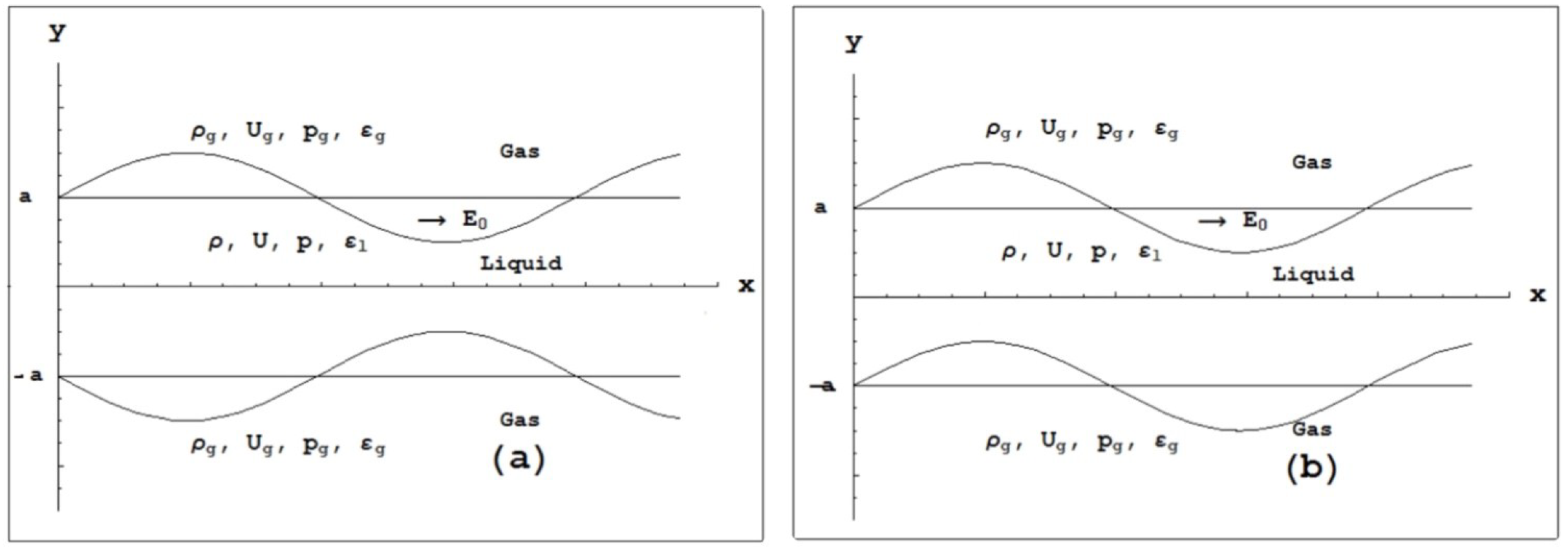
2. Formulation and Perturbation Equations

We consider a viscoelastic dielectric liquid sheet of couple-stress type whose thickness is $2a$ that issues from a nozzle at a velocity $U_{0l}$ and has a density ${\rho }_l$, pressure $p_l$, dielectric constant ${ϵ}_l$, kinematic viscosity $v_l\left(={\mu }_l/{\rho }_l\right)$, and kinematic viscoelasticity $v_l^{\prime }\left(={\mu }_l^{\prime }/{\rho }_l\right)$, where ${\mu }_l$ and ${\mu }_l^{\prime }$ are the dynamic viscosity and dynamic viscoelasticity, respectively. This liquid sheet is surrounded by a moving inviscid dielectric gas whose velocity is $U_{0g}$ and has a density ${\rho }_g$, pressure $p_g$, dielectric constant ${ϵ}_g$ and kinematic viscosity ${\nu }_g,$ as shown in Figure 1. The whole system is influenced by the presence of an electric field ${\mathit{E}}_0$ parallel to the interfaces $y=\pm a$, and streaming through a porous medium whose porosity is $\epsilon$, and whose permeability is $k_1$.

The governing equations in three-dimensional Cartesian coordinates are the equation of continuity, Navier–Stokes equation of motion, and Maxwell’s equations in both liquid and gas media defined by [32,33]

$$\frac{\partial u_l}{\partial x}+\frac{\partial v_l}{\partial y}+\frac{\partial w_l}{\partial z}=0$$

(1)

$$\frac{1}{\epsilon }\frac{\partial u_l}{\partial t}+\frac{1}{{\epsilon }^2}{U}_{0l}\frac{\partial u_l}{\partial x}=-\frac{1}{{\rho }_l}\frac{\partial p_l}{\partial x}-\frac{1}{k_1}\left(v_l-v_l^{\prime }{\nabla }^2\right)u_l$$

(2)

$$\frac{1}{\epsilon }\frac{\partial v_l}{\partial t}+\frac{1}{{\epsilon }^2}{U}_{0l}\frac{\partial v_l}{\partial x}=-\frac{1}{{\rho }_l}\frac{\partial p_l}{\partial y}-\frac{1}{k_1}\left(v_l-v_l^{\prime }{\nabla }^2\right)v_l$$

(3)

$$\frac{1}{\epsilon }\frac{\partial w_l}{\partial t}+\frac{1}{{\epsilon }^2}{U}_{0l}\frac{\partial w_l}{\partial x}=-\frac{1}{{\rho }_l}\frac{\partial p_l}{\partial z}-\frac{1}{k_1}\left(v_l-v_l^{\prime }{\nabla }^2\right)w_l$$

(4)

and

$$\frac{\partial u_g}{\partial x}+\frac{\partial v_g}{\partial y}+\frac{\partial w_g}{\partial z}=0$$

(5)

$$\frac{1}{\epsilon }\frac{\partial u_g}{\partial t}+\frac{1}{{\epsilon }^2}{U}_{0g}\frac{\partial u_g}{\partial x}=-\frac{1}{{\rho }_g}\frac{\partial p_g}{\partial x}-\frac{v_g}{k_1}{u}_g$$

(6)

$$\frac{1}{\epsilon }\frac{\partial v_g}{\partial t}+\frac{1}{{\epsilon }^2}{U}_{0g}\frac{\partial v_g}{\partial x}=-\frac{1}{{\rho }_g}\frac{\partial p_g}{\partial y}-\frac{v_g}{k_1}{v}_g$$

(7)

$$\frac{1}{\epsilon }\frac{\partial w_g}{\partial t}+\frac{1}{{\epsilon }^2}{U}_{0g}\frac{\partial w_g}{\partial x}=\frac{1}{{\rho }_g}\frac{\partial p_g}{\partial z}-\frac{v_g}{k_1}{w}_g$$

(8)

$$\nabla ·\left({ϵ}_j{\mathit{E}}_j\right)=0$$

(9)

$$\nabla \times {\mathit{E}}_j=0$$

(10)

Maxwell’s equations of motion are used to derive Equations (9) and (10) by assuming that the quasi-static approximation is applicable in this problem, and so the electric field ${\mathit{E}}_j$ can be calculated from the gradient of a scalar electric potential ${\psi }_j$. The subscripts $(j=l,g)$ signify the liquid sheet and the gas.

The flow has been divided into a steady flow and a time dependent perturbation. The total electric field will be defined as ${\mathit{E}}_j={\mathit{E}}_0\mathit{i}-\nabla {\psi }_j$, then Equation (9) indicates that electric potentials ${\psi }_j$ in the two regions satisfy the following Laplace’s equations

$${\nabla }^2{\psi }_j=0$$

(11)

Let $u_{1j},v_{1j},w_{1j},p_{1j}$, and ${\psi }_{1j}$ where $(j=l,g)$, denote perturbations in the fluid velocity components $u_{0j},v_{0j},w_{0j}$, the pressure $p_{0j}$, and the electric potentials ${\psi }_{0j}$. Hence, we also can write

$$u_j=u_{0j}+u_{1j},v_j=v_{1j},w_j=w_{1j},p_j=p_{0j}+p_{1j}\mathrm{and}{\psi }_j={\psi }_{0j}+{\psi }_{1j}$$

Substituting for the above quantities into Equations (1)–(8), and (11), we obtain the following perturbed equations in the liquid sheet medium

$$\frac{\partial u_{1l}}{\partial x}+\frac{\partial v_{1l}}{\partial y}+\frac{\partial w_{1l}}{\partial z}=0$$

(12)

$$\frac{1}{{\epsilon }^2}\left[\epsilon \frac{\partial u_{1l}}{\partial t}+U_{0l}\frac{\partial u_{1l}}{\partial x}+\frac{{\epsilon }^2}{k_1}\left(v_l-v_l^{\prime }{\nabla }^2\right)u_{1l}\right]=-\frac{1}{{\rho }_l}\frac{\partial p_{1l}}{\partial x}$$

(13)

$$\frac{1}{{\epsilon }^2}\left[\epsilon \frac{\partial v_l}{\partial t}+U_{0l}\frac{\partial v_{1l}}{\partial x}+\frac{{\epsilon }^2}{k_1}\left(v_l-v_l^{\prime }{\nabla }^2\right)v_{1l}\right]=-\frac{1}{{\rho }_l}\frac{\partial p_{1l}}{\partial y}$$

(14)

$$\frac{1}{{\epsilon }^2}\left[\epsilon \frac{\partial w_{1l}}{\partial x}+U_{0l}\frac{\partial w_{1l}}{\partial x}+\frac{{\epsilon }^2}{k_1}\left(v_l-v_l^{\prime }{\nabla }^2\right)w_{1l}\right]=-\frac{1}{{\rho }_l}\frac{\partial p_{1l}}{\partial z}$$

(15)

and in the gas region as

$$\frac{\partial u_{1g}}{\partial x}+\frac{\partial v_{1g}}{\partial y}+\frac{\partial w_{1g}}{\partial z}=0$$

(16)

$$\frac{1}{{\epsilon }^2}\left[\epsilon \frac{\partial u_{1g}}{\partial t}+U_{0g}\frac{\partial u_{1g}}{\partial x}+\frac{{\epsilon }^2{v}_g}{k_1}{u}_{1g}\right]=-\frac{1}{{\rho }_g}\frac{\partial p_{1g}}{\partial x}$$

(17)

$$\frac{1}{{\epsilon }^2}\left[\epsilon \frac{\partial v_{1g}}{\partial t}+U_{0g}\frac{\partial v_{1g}}{\partial x}+\frac{{\epsilon }^2{v}_g}{k_1}{v}_{1g}\right]=-\frac{1}{{\rho }_g}\frac{\partial p_{1g}}{\partial y}$$

(18)

$$\frac{1}{{\epsilon }^2}\left[\epsilon \frac{\partial v_{1g}}{\partial t}+U_{0g}\frac{\partial v_{1g}}{\partial x}+\frac{{\epsilon }^2{v}_g}{k_1}{w}_{1g}\right]=-\frac{1}{{\rho }_g}\frac{\partial p_{1g}}{\partial z}$$

(19)

Together with the electric potential equations in both regions

$${\nabla }^2{\psi }_{1l}=0\mathrm{and}{\nabla }^2{\psi }_{1g}=0$$

(20)

3. Normal Modes Analysis and Solutions

We seek solutions to Equations (13)–(20) in the liquid and gas medium whose dependency on $x,y,z,$ and t is of the type [34] to analyze the disturbance into normal modes analysis

$$\left(u_{1l},v_{1l},w_{1l},p_{1l},{\psi }_{1l}\right)=\left(U_l,V_l,W_l,P_l,{\Psi }_l\right)exp[i(kx+nz)+\omega t]$$

(21)

$$\left(u_{1g},v_{1g},w_{1g},p_{1g},{\psi }_{1g}\right)=\left(U_g,V_g,W_g,P_g,{\Psi }_g\right)exp[i(kx+nz)+\omega t]$$

(22)

where $U_l,V_l,W_l,P_l,{\Psi }_l$ and $U_g,V_g,W_g,P_g,{\Psi }_g$ are functions of y only; k and n are the wave numbers in the x and z, respectively, and $\omega ={\omega }_r+i{\omega }_i$ is the complex frequency.

The interface displacement is given by

$$\eta ={\eta }_{0}exp[i(kx+nz)+\omega t]$$

(23)

Substituting Equations (21) and (22) into Equations (13)–(20), we obtain in the liquid sheet medium the equation

$$ik{U}_l+D{V}_l+in{W}_l=0$$

(24)

$$\left\{\left(\epsilon \omega +ik{U}_{0l}\right)+\frac{{\epsilon }^2}{k_1}\left[v_l-v_l^{\prime }\left(D^2-m^2\right)\right]\right\}{U}_l=-\frac{{\epsilon }^2}{{\rho }_l}\left(ik{P}_l\right)$$

(25)

$$\left\{\left(\epsilon \omega +ik{U}_{0l}\right)+\frac{{\epsilon }^2}{k_1}\left[v_l-v_l^{\prime }\left(D^2-m^2\right)\right]\right\}{V}_l=-\frac{{\epsilon }^2}{{\rho }_l}\left(D{P}_l\right)$$

(26)

$$\left\{\left(\epsilon \omega +ik{U}_{0l}\right)+\frac{{\epsilon }^2}{k_1}\left[v_l-v_l^{\prime }\left(D^2-m^2\right)\right]\right\}{W}_l=-\frac{{\epsilon }^2}{{\rho }_l}\left(in{P}_l\right)$$

(27)

$$\left(D^2-m^2\right){\Psi }_l=0$$

(28)

where $m^2=k^2+n^2$. Similarly, in the gas medium we obtain the following equations

$$ik{U}_g+D{V}_g+in{W}_g=0$$

(29)

$$\left[\left(\epsilon \omega +ik{U}_{0g}\right)+\frac{{\epsilon }^2{v}_g}{k_1}\right]U_g=-\frac{{\epsilon }^2}{{\rho }_l}\left(ik{P}_g\right)$$

(30)

$$\left[\left(\epsilon \omega +ik{U}_{0g}\right)+\frac{{\epsilon }^2{v}_g}{k_1}\right]V_g=-\frac{{\epsilon }^2}{{\rho }_l}\left(D{P}_g\right)$$

(31)

$$\left[\left(\epsilon \omega +ik{U}_{0g}\right)+\frac{{\epsilon }^2{v}_g}{k_1}\right]W_g=-\frac{{\epsilon }^2}{{\rho }_l}\left(in{P}_g\right)$$

(32)

$$\left(D^2-m^2\right){\Psi }_g=0$$

(33)

Multiplying Equation (25) by $ik$, operate by the operator D on Equation (26), multiply Equation (27) by $in$, and add the obtained three equations. Afterwards, using Equation (24), we obtain

$$\left(D^2-m^2\right)P_l=0$$

(34)

The solution of Equation (34) is given by

$$p_{1l}=\left[C_1{e}^{my}+C_2{e}^{-my}\right]exp[i(kx+nz)+\omega t]$$

(35)

where $C_1$ and $C_2$ are constants of integration to be determined. Then, we can write

Equation (25) can be written in the form

$$\left(D^2-s^2\right)U_l=\frac{ik{k}_1}{{\rho }_l{v}_l^{\prime }}\left(C_1{e}^{my}+C_2{e}^{-my}\right)$$

(36)

where

$$s^2=m^2+\frac{k_1\left(\epsilon \omega +ik{U}_{ol}\right)+{\epsilon }^2{v}_l}{{\epsilon }^2{v}_l^{\prime }}$$

(37)

Hence, the general solution of nonhomogeneous differential Equation (36) is given by

$$u_{1l}=\left[C_3{e}^{sy}+C_4{e}^{-sy}+\frac{ik{k}_1}{{\rho }_l{v}_l^{\prime }}\left(\frac{C_1{e}^{my}+C_2{e}^{-my}}{m^2-s^2}\right)\right]exp[i(kx+nz)+\omega t]$$

(38)

Similarly, Equations (26) and (27) can be written in the form

$$\left(D^2-s^2\right)V_l=\frac{m{k}_1}{{\rho }_l{v}_l^{\prime }}\left(C_1{e}^{my}-C_2{e}^{-my}\right)$$

(39)

$$\left(D^2-s^2\right)W_l=\frac{in{k}_1}{{\rho }_l{v}_l^{\prime }}\left(C_1{e}^{my}+C_2{e}^{-my}\right)$$

(40)

The solutions to nonhomogeneous differential Equations (39) and (40) are

$$v_{1l}=\left[C_5{e}^{sy}+C_6{e}^{-sy}+\frac{m{k}_1}{{\rho }_l{v}_l^{\prime }}\left(\frac{C_1{e}^{my}-C_2{e}^{-my}}{m^2-s^2}\right)\right]exp[i(kx+nz)+\omega t]$$

(41)

$$w_{1l}=\left[C_7{e}^{sy}+C_8{e}^{-sy}+\frac{in{k}_1}{{\rho }_l{v}_l^{\prime }}\left(\frac{C_1{e}^{my}+C_2{e}^{-my}}{m^2-s^2}\right)\right]exp[i(kx+nz)+\omega t]$$

(42)

where $C_3$–$C_8$ are constants to determined. Furthermore, from Equations (29)–(32), we obtain

$$\left(D^2-m^2\right)P_g=0$$

(43)

The solution of Equations (28), (33) and (43) can be written in the forms

Hence, we can write

$$p_{1g}=\left[C_9{e}^{my}+C_{10}{e}^{-my}\right]exp[i(kx+nz)+\omega t]$$

(44)

$${\psi }_{1l}=\left[A_1{e}^{my}+A_2{e}^{-my}\right]exp[i(kx+nz)+\omega t]$$

(45)

$${\psi }_{1g}=\left[B_1{e}^{my}+B_2{e}^{-my}\right]exp[i(kx+nz)+\omega t]$$

(46)

where $A_1,A_2,B_1,B_2,C_9$ and $C_{10}$ are constants of integration to be determined.

4. Boundary Conditions

If the disturbance is antisymmetric or symmetric, the required boundary conditions for the considered system are different. The upper and lower interfaces are used for antisymmetric disturbances, for example at $y=\pm a$ is described by $y=a+\eta$ and $y=-a+\eta$, respectively, while for symmetric disturbance, the two interfaces are described, respectively, by $y=a+\eta$ and $y=$$-a-\eta$, where $\eta$ is defined by Equation (23).

The antisymmetric disturbance case boundary conditions at $y=\pm a$ are [8,13]

• The kinematic boundary condition should be satisfied at the two interfaces, which states that the normal velocities of the liquid sheet at $y=\pm a$ are

  $$v_{1l}=\epsilon \frac{\partial \eta }{\partial t}+U_{0l}\frac{\partial \eta }{\partial x}\mathrm{at}y=\pm a$$

  (47)

  and for the gas medium, this condition yields

  $$v_{1g}=\epsilon \frac{\partial \eta }{\partial t}+U_{0g}\frac{\partial \eta }{\partial x}\mathrm{at}y=a$$

  (48)
• The perturbed velocity of the gas far away from the interface should be vanishes, i.e.,

  $$v_{1g}=0\mathrm{at}y\to \pm \infty$$

  (49)
• The stress tensor’s tangential component must be continuous at the interfaces, i.e.,

  $${\tau }_{yx}=\frac{1}{k_1}\left({\mu }_l-{\mu }_l^{\prime }{\nabla }^2\right)\left(\frac{\partial u_{1l}}{\partial y}+\frac{\partial v_{1l}}{\partial x}\right)=0\mathrm{at}y=\pm a$$

  (50)

  $${\tau }_{yz}=\frac{1}{k_1}\left({\mu }_l-{\mu }_l^{\prime }{\nabla }^2\right)\left(\frac{\partial v_{1l}}{\partial z}+\frac{\partial w_{1l}}{\partial y}\right)=0\mathrm{at}y=\pm a$$

  (51)
• At the interfaces, the electric field’s tangential component is continuous.

  $$\frac{\partial {\psi }_{1l}}{\partial x}=\frac{\partial {\psi }_{1g}}{\partial x}\mathrm{at}y=\pm a$$

  (52)
• At interfaces, the electric displacement’s normal component is continuous.

  $${ϵ}_l\frac{\partial {\psi }_{1l}}{\partial y}-{ϵ}_g\frac{\partial {\psi }_{1g}}{\partial y}=ik\eta E_0\left({ϵ}_l-{ϵ}_g\right)\mathrm{at}y=\pm a$$

  (53)
• The stress tensor normal component is broken up at the interface by the surface tension coefficient, i.e.,

  $$-p_{1l}+{ϵ}_l{E}_0\frac{\partial {\psi }_{1l}}{\partial x}+2\left({\mu }_l-{\mu }_l^{\prime }{\nabla }^2\right)\frac{\partial v_{1l}}{\partial y}=-p_{1g}+{ϵ}_g{E}_0\frac{\partial {\psi }_{1g}}{\partial x}+p_{\sigma }\mathrm{at}y=\pm a$$

  (54)

  where $p_{\sigma }$ is the pressure due to the surface tension $\sigma$.
  Please note that for symmetric disturbances the boundary conditions that change forms are

• The kinematic boundary condition (47) and the electric displacement boundary condition (53) at $y=-a$ take the forms

  $$v_{1l}=-\left(\epsilon \frac{\partial \eta }{\partial t}+U_{0l}\frac{\partial \eta }{\partial x}\right)\mathrm{at}y=-a$$

  (55)

  $$v_{1g}=-\left(\epsilon \frac{\partial \eta }{\partial t}+U_{0g}\frac{\partial \eta }{\partial x}\right)\mathrm{at}y=-a$$

  (56)

  $${ϵ}_l\frac{\partial {\psi }_{1l}}{\partial y}-{ϵ}_g\frac{\partial {\psi }_{1g}}{\partial y}=-ik\eta E_0\left({ϵ}_l-{ϵ}_g\right)\mathrm{at}y=-a$$

  (57)

5. The Antisymmetric Disturbance Case

For each of the fluid sheets and gas media (upper and lower phases), as well as the differential equation representing the influence of the electric field, we will try to find solutions in this section as follows:

5.1. Solutions in the Liquid Sheet Phase

The kinematic boundary condition (47), on using Equations (23) and (41), can be written at the two interfaces in the form

$$C_5{e}^{sa}+C_6{e}^{-sa}+\frac{m{k}_1}{{\rho }_l{v}_l^{\prime }}\frac{\left(C_1{e}^{ma}-C_2{e}^{-ma}\right)}{\left(m^2-s^2\right)}=\left(\epsilon \omega +ik{U}_{0l}\right){\eta }_0$$

(58)

$$C_5{e}^{-sa}+C_6{e}^{sa}+\frac{m{k}_1}{{\rho }_l{v}_l^{\prime }}\frac{\left(C_1{e}^{-ma}-C_2{e}^{ma}\right)}{\left(m^2-s^2\right)}=\left(\epsilon \omega +ik{U}_{0l}\right){\eta }_0$$

(59)

Solving Equations (58) and (59), we obtain

$$C_5=\frac{\left(\epsilon \omega +ik{U}_{0l}\right){\eta }_0}{2cosh\left(sa\right)}-\frac{m{k}_1\left\{C_{1}sinh\left[(s+m)a\right]-C_{2}sinh\left[(s-m)a\right]\right\}}{{\rho }_l{v}_l^{\prime }\left(m^2-s^2\right)sinh\left(2sa\right)}$$

(60)

$$C_6=\frac{\left(\epsilon \omega +ik{U}_{0l}\right){\eta }_0}{2cosh\left(sa\right)}-\frac{m{k}_1\left\{C_{1}sinh\left[(s-m)a\right]-C_{2}sinh\left[(s+m)a\right]\right\}}{{\rho }_l{v}_l^{\prime }\left(m^2-s^2\right)sinh\left(2sa\right)}$$

(61)

The tangential stress boundary condition (50), on using Equations (38), (41), (58) and (59), can be written at the two interfaces in the form

$$C_{3}s{e}^{sa}-C_{4}s{e}^{-sa}+\frac{ik{k}_{1}m\left(C_1{e}^{ma}-C_2{e}^{-ma}\right)}{{\rho }_l{v}_l^{\prime }\left(m^2-s^2\right)}+ik\left(\epsilon \omega +ik{U}_{0l}\right){\eta }_0=0$$

(62)

$$C_{3}s{e}^{-sy}-C_{4}s{e}^{sa}+\frac{ik{k}_{1}m\left(C_1{e}^{-ma}-C_2{e}^{ma}\right)}{{\rho }_l{v}_l^{\prime }\left(m^2-s^2\right)}+ik\left(\epsilon \omega +ik{U}_{0l}\right){\eta }_0=0$$

(63)

Solving Equations (62) and (63), we obtain

$$C_3=-\frac{ik{k}_{1}m\left\{C_{1}sinh\left[(s+m)a\right]-C_{2}sinh\left[(s-m)a\right]\right\}}{s{\rho }_l{v}_l^{\prime }\left(m^2-s^2\right)sinh\left(2sa\right)}-\frac{ik\left(\epsilon \omega +ik{U}_{0l}\right){\eta }_0}{2scosh\left(sa\right)}$$

(64)

$$C_4=\frac{ik{k}_{1}m\left\{C_{1}sinh\left[(s-m)a\right]-C_{2}sinh\left[(s+m)a\right]\right\}}{s{\rho }_l{v}_l^{\prime }\left(m^2-s^2\right)sinh\left(2sa\right)}+\frac{ik\left(\epsilon \omega +ik{U}_{0l}\right){\eta }_0}{2scosh\left(sa\right)}$$

(65)

The tangential stress boundary condition (51), on using Equations (41), (42), (58) and (59), can be written at the two interfaces in the form

$$s\left(C_7{e}^{sa}-C_8{e}^{-sa}\right)=-in\left(\epsilon \omega +ik{U}_{0l}\right){\eta }_0-\frac{inm{k}_1\left(C_1{e}^{ma}-C_2{e}^{-ma}\right)}{{\rho }_l{v}_l^{\prime }\left(m^2-s^2\right)}$$

(66)

$$s\left(C_7{e}^{-sa}-C_8{e}^{sa}\right)=-in\left(\epsilon \omega +ik{U}_{0l}\right){\eta }_0-\frac{inm{k}_1\left(C_1{e}^{-ma}-C_2{e}^{ma}\right)}{{\rho }_l{v}_l^{\prime }\left(m^2-s^2\right)}$$

(67)

Solving Equations (66) and (67), we obtain

$$C_7=-\frac{in\left(\epsilon \omega +ik{U}_{0l}\right){\eta }_0}{2scosh\left(sa\right)}-\frac{inm{k}_1\left\{C_{1}sinh\left[(s+m)a\right]-C_{2}sinh\left[(s-m)a\right]\right\}}{s{\rho }_l{v}_l^{\prime }\left(m^2-s^2\right)sinh\left(2sa\right)}$$

(68)

$$C_8=\frac{in\left(\epsilon \omega +ik{U}_{0l}\right){\eta }_0}{2scosh\left(sa\right)}+\frac{\left.inm{k}_1\left\{C_{1}sinh\left[(s-m)a\right]-C_{2}sinh\left[(s+m)a\right]\right]\right\}}{s{\rho }_l{v}_l^{\prime }\left(m^2-s^2\right)sinh\left(2sa\right)}$$

(69)

The equation of continuity (12) at $y=\pm a$, on using Equations (38), (41), and (42) can be written in the form

$$\begin{array}{cc}\hfill \left[{sinh}^2\left(sa\right)cosh\left(ma\right)\right.& \left.+{cosh}^2\left(sa\right)sinh\left(ma\right)\right]C_1\hfill \\ \hfill & -\left[{sinh}^2\left(sa\right)cosh\left(ma\right)-{cosh}^2\left(sa\right)sinh\left(ma\right)\right]C_2\hfill \\ \hfill & +\frac{{\rho }_l{v}_l^{\prime }}{k_{1}m}\left(m^2+s^2\right)\left(\epsilon \omega +ik{U}_{0l}\right){\eta }_0{sinh}^2\left(sa\right)=0\hfill \end{array}$$

(70)

and

$$\begin{array}{cc}\hfill \left[{sinh}^2\left(sa\right)cosh\left(ma\right)\right.& \left.-{cosh}^2\left(sa\right)sinh\left(ma\right)\right]C_1\hfill \\ \hfill & -\left[{sinh}^2\left(sa\right)cosh\left(ma\right)+{cosh}^2\left(sa\right)sinh\left(ma\right)\right]C_2\hfill \\ \hfill & +\frac{{\rho }_l{v}_l^{\prime }}{k_{1}m}\left(m^2+s^2\right)\left(\epsilon \omega +ik{U}_{0l}\right){\eta }_0{sinh}^2\left(sa\right)=0\hfill \end{array}$$

(71)

Solving Equations (70) and (71), we obtain

$$C_1=-C_2=-\frac{{\rho }_l{v}_l^{\prime }\left(m^2+s^2\right)\left(\epsilon \omega +ik{U}_{0l}\right){\eta }_0}{2k_{1}mcosh\left(ma\right)}$$

(72)

Substitute from Equations (72) into Equations (64), (65), (60), (61), (68), and (69), respectively, we obtain

$$C_3=-C_4=\frac{iks\left(\epsilon \omega +ik{U}_{0l}\right){\eta }_0}{\left(m^2-s^2\right)cosh\left(sa\right)}$$

(73)

$$C_5=C_6=\frac{m^2\left(\epsilon \omega +ik{U}_{0l}\right){\eta }_0}{\left(m^2-s^2\right)cosh\left(sa\right)}$$

(74)

$$C_7=-C_8=-\frac{ins\left(\epsilon \omega +ik{U}_{0l}\right){\eta }_0}{\left(m^2-s^2\right)cosh\left(sa\right)}$$

(75)

Substitute from Equations (72) and (75) into Equations (38), (41) and (42) we obtain

$${\mathrm{p}}_{1l}=-\frac{{\rho }_l{v}_l^{\prime }\left(m^2+s^2\right)\left(\epsilon \omega +ik{U}_{0l}\right){\eta }_{0}sinh\left(my\right)}{k_{1}mcosh\left(ma\right)}exp[i(kx+nz)+\omega t]$$

(76)

and

$$u_{1l}=\frac{ik\left(\epsilon \omega +ik{U}_{0l}\right){\eta }_0}{\left(m^2-s^2\right)}\left[\frac{2ssinh\left(sy\right)}{cosh\left(sa\right)}-\frac{\left(m^2+s^2\right)sinh\left(my\right)}{mcosh\left(ma\right)}\right]exp[i(kx+nz)+\omega t]$$

(77)

$$v_{1l}=\frac{\left(\epsilon \omega +ik{U}_{0l}\right){\eta }_0}{\left(m^2-s^2\right)}\left[\frac{2m^{2}cosh\left(sy\right)}{cosh\left(sa\right)}-\frac{\left(m^2+s^2\right)cosh\left(my\right)}{cosh\left(ma\right)}\right]exp[i(kx+nz)+\omega t]$$

(78)

$$w_{1l}=\frac{in\left(\epsilon w+ik{U}_{0l}\right){\eta }_0}{\left(m^2-s^2\right)}\left[\frac{2ssinh\left(sy\right))}{cosh\left(sa\right)}-\frac{\left.\left(m^2+s^2\right)sinh\left(my\right)\right)}{mcosh\left(ma\right)}\right]exp[i(kx+nz)+\omega t]$$

(79)

5.2. Solutions in the Gas Medium (in the Upper and Lower Phases)

Substitute form Equation (44) into Equations (30)–(32), we obtain

$$u_{1g}=-\frac{ik{\epsilon }^2\left(C_9{e}^{my}+C_{10}{e}^{-my}\right)}{{\rho }_g\left[\left(\epsilon \omega +ik{U}_{0g}\right)+\frac{{\epsilon }^2{v}_g}{k_1}\right]}$$

(80)

$$v_{1g}=-\frac{m{\epsilon }^2\left(C_9{e}^{my}-C_{10}{e}^{-my}\right)}{{\rho }_g\left[\left(\epsilon \omega +ik{U}_{0g}\right)+\frac{{\epsilon }^2{v}_g}{k_1}\right]}$$

(81)

$$w_{1g}=-\frac{in{\epsilon }^2\left(C_9{e}^{my}+C_{10}{e}^{-my}\right)}{{\rho }_g\left[\left(\epsilon \omega +ik{U}_{0g}\right)+\frac{{\epsilon }^2{v}_g}{k_1}\right]}$$

(82)

Using the kinematic boundary condition (48), and condition (49) in the two regions $(y\to \infty )$ and $(y\to -\infty )$, the in the upper gas region we obtain $C_9=0$, while in the lower gas region, we have $C_{10}=0$. Then in the upper gas region $(y\ge a)$, we have

$$C_{10}=\frac{{\rho }_g\left(\epsilon \omega +ik{U}_{0g}\right){\eta }_0}{m{\epsilon }^2}\left[\left(\epsilon \omega +ik{U}_{0g}\right)+\frac{{\epsilon }^2{v}_g}{k_1}\right]e^{ma}$$

(83)

Therefore, in the upper gas medium, Equation (44) gives

$$p_{1g}^u=\frac{{\rho }_g\left(\epsilon \omega +ik{U}_{0g}\right){\eta }_0}{m{\epsilon }^2}\left[\left(\epsilon \omega +ik{U}_{0g}\right)+\frac{{\epsilon }^2{v}_g}{k_1}\right]exp\left[m(a-y)\right]exp[i(kx+nz)+\omega t]$$

(84)

Furthermore, Equations (80)–(82) yield the velocity component for $(y\ge a)$ as

$$u_{1g}^u=-\frac{ik\left(\epsilon \omega +ik{U}_{0g}\right){\eta }_0}{m}exp\left[m(a-y)\right]exp[i(kx+nz)+\omega t]$$

(85)

$$v_{1g}^u=\left(\epsilon \omega +ik{U}_{0g}\right){\eta }_{0}exp\left[m(a-y)\right]exp[i(kx+nz)+\omega t]$$

(86)

$$w_{1g}^u=-\frac{ik\left(\epsilon \omega +ik{U}_{0g}\right){\eta }_0}{m}exp\left[m(a-y)\right]exp[i(kx+nz)+\omega t]$$

(87)

Similarly, in the lower gas region $(y\le -a)$, we have

$$C_9=-\frac{{\rho }_g\left(\epsilon \omega +ik{U}_{0g}\right){\eta }_0}{m{\epsilon }^2}\left[\left(\epsilon \omega +ik{U}_{0g}\right)+\frac{{\epsilon }^2{v}_g}{k_1}\right]e^{ma}$$

(88)

Therefore, in the lower gas medium, Equation (44) gives

$$\begin{array}{cc}\hfill p_{1g}^l=-\frac{{\rho }_l\left(\epsilon \omega +ik{U}_{0g}\right){\eta }_0}{m{\epsilon }^2}& \left[\left(\epsilon \omega +ik{U}_{0g}\right)+\frac{{\epsilon }^2{v}_g}{k_1}\right]exp\left[m(a+y)\right]exp[i(kx+nz)+\omega t]\hfill \end{array}$$

(89)

Hence, Equations (80)–(82) yield

$$u_{1g}^l=\frac{ik\left(\epsilon \omega +ik{U}_{0g}\right){\eta }_0}{m}exp\left[m(a+y)\right]exp[i(kx+nz)+\omega t]$$

(90)

$$v_{1g}^l=\left(\epsilon \omega +ik{U}_{0g}\right){\eta }_{0}exp\left[m(a+y)\right]exp[i(kx+nz)+\omega t]$$

(91)

$$w_{1g}^l=\frac{in\left(\epsilon \omega +ik{U}_{0g}\right){\eta }_0}{m}exp\left[m(a+y)\right]exp[i(kx+nz)+\omega t]$$

(92)

Furthermore, the pressure due to the presence of surface tension is given by

$$p_{\sigma }=\sigma \left(\frac{{\partial }^2\eta }{\partial x^2}+\frac{{\partial }^2\eta }{\partial z^2}\right)=-\sigma m^2{\eta }_{0}exp[i(kx+nz)+\omega t]$$

(93)

5.3. Solutions of the Electric Field (in the Upper and Lower Phases)

From Equation (46), since ${\psi }_{1g}\to 0$ as $y\to \pm \infty$, then in the upper gas region $(y\ge a)$, we take $B_1=0$, while in the lower gas region $(y\le -a)$, we take $B_2=0$. Then substituting from Equation (45) of the liquid phase and Equation (46) for the gas phase (in the upper and lower regions) into the boundary conditions (52) and (53) at $y=\pm a$, we obtain

$$\left(A_1{e}^{ma}+A_2{e}^{-ma}\right)=B_2{e}^{-ma}$$

(94)

$$\left(A_1{e}^{-ma}+A_2{e}^{ma}\right)=B_1{e}^{-ma}$$

(95)

$${ϵ}_{l}m\left(A_1{e}^{ma}-A_2{e}^{-ma}\right)+{ϵ}_{g}m{B}_2{e}^{-ma}=ik{\eta }_0{E}_0\left({ϵ}_l-{ϵ}_g\right)$$

(96)

$${ϵ}_{l}m\left(A_1{e}^{-ma}-A_2{e}^{ma}\right)-{ϵ}_{g}m{B}_1{e}^{-ma}=ik{\eta }_0{E}_0\left({ϵ}_l-{ϵ}_g\right)$$

(97)

Now, solving Equations (94)–(97), we obtain

$$A_1=-A_2=\frac{ik{\eta }_0{E}_0\left({ϵ}_l-{ϵ}_g\right)}{2mcosh\left(ma\right)\left[{ϵ}_l+{ϵ}_{g}tanh\left(ma\right)\right]}$$

(98)

and

$$B_1=-B_2=-\frac{ik{\eta }_0{E}_0\left({ϵ}_l-{ϵ}_g\right)e^{ma}tanh\left(ma\right)}{m\left[{ϵ}_l+{ϵ}_{g}tanh\left(ma\right)\right]}$$

(99)

Therefore, the solutions (45) and (46) can be written in the form

$${\psi }_{1l}=\frac{ik{\eta }_0{E}_0\left({ϵ}_l-{ϵ}_g\right)sinh\left(my\right)}{m\left[{ϵ}_l+{ϵ}_{g}tanh\left(ma\right)\right]cosh\left(ma\right)}exp[i(kx+nz)+\omega t]$$

(100)

$${\psi }_{1g}^u=\frac{ik{\eta }_0{E}_0\left({ϵ}_l-{ϵ}_g\right)tanh\left(ma\right)}{m\left[{ϵ}_l+{ϵ}_{g}tanh\left(ma\right)\right]}exp\left[m(a-y)\right]exp[i(kx+nz)+\omega t]$$

(101)

$${\psi }_{1g}^l=-\frac{ik{\eta }_0{E}_0\left({ϵ}_l-{ϵ}_g\right)tanh\left(ma\right)}{m\left[{ϵ}_l+{ϵ}_{g}tanh\left(ma\right)\right]}exp\left[m(a+y)\right]exp[i(kx+nz)+\omega t]$$

(102)

6. The Symmetric Disturbance Case

In this section, we will try to obtain the solutions for the above-mentioned differential equations describing each of the liquid sheet medium, and the gas medium (in the upper and lower phases), together with the solution of the differential equation of the electric field, in the corresponding case of symmetric disturbance. We note that the obtained solutions for the gas medium in this case is found to be similar to the solutions for the previous case of antisymmetric disturbances and will not be given here.

6.1. Solutions in the Liquid Sheet Phase

Following the same procedure shown in the previous case of antisymmetric disturbance together with the help of Equation (55) at $y=-a$, we obtain

$$C_1=C_2=-\frac{{\rho }_l{v}_l^{\prime }\left(m^2+s^2\right)\left(\epsilon \omega +ik{U}_{0l}\right){\eta }_0}{2k_{1}msinh\left(ma\right)}$$

(103)

$$C_3=C_4=\frac{iks\left(\epsilon \omega +ik{U}_{0l}\right){\eta }_0}{\left(m^2-s^2\right)sinh\left(sa\right)}$$

(104)

$$C_5=-C_6=\frac{m^2\left(\epsilon \omega +ik{U}_{0l}\right){\eta }_0}{\left(m^2-s^2\right)sinh\left(sa\right)}$$

(105)

$$C_7=C_8=\frac{ins\left(\epsilon \omega +ik{U}_{0l}\right){\eta }_0}{\left(m^2-s^2\right)sinh\left(sa\right)}$$

(106)

Hence, we have the following solution

$${\mathrm{p}}_{1l}=-\frac{{\rho }_l{v}_l^{\prime }\left(m^2+s^2\right)\left(\epsilon \omega +ik{U}_{0l}\right){\eta }_{0}cosh\left(my\right)}{k_{1}msinh\left(ma\right)}exp[i(kx+nz)+\omega t]$$

(107)

$$u_{1l}=\frac{ik\left(\epsilon \omega +ik{U}_{0l}\right){\eta }_0}{\left(m^2-s^2\right)}\left[\frac{2scosh\left(sy\right)}{sinh\left(sa\right)}-\frac{\left(m^2+s^2\right)cosh\left(my\right)}{msinh\left(ma\right)}\right]exp[i(kx+nz)+\omega t]$$

(108)

$$v_{1l}=\frac{\left(\epsilon \omega +ik{U}_{0l}\right){\eta }_0}{\left(m^2-s^2\right)}\left[\frac{2m^{2}sinh\left(sy\right)}{sinh\left(sa\right)}-\frac{\left(m^2+s^2\right)sinh\left(my\right)}{sinh\left(ma\right)}\right]exp[i(kx+nz)+\omega t]$$

(109)

$$w_{1l}=\frac{in\left(\epsilon w+ik{U}_{0l}\right){\eta }_0}{\left(m^2-s^2\right)}\left[\frac{2scosh\left(sy\right))}{sinh\left(sa\right)}-\frac{\left.\left(m^2+s^2\right)cosh\left(my\right)\right)}{msinh\left(ma\right)}\right]exp[i(kx+nz)+\omega t]$$

(110)

6.2. Solutions of the Electric Field (in the Upper and Lower Phases)

Following the same procedure given in the previous case of antisymmetric disturbance, together with the help of Equation (57) at $y=-a$, we obtain

$$A_1=A_2=\frac{ik{\eta }_0{E}_0\left({ϵ}_l-{ϵ}_g\right)}{2msinh\left(ma\right)\left[{ϵ}_l+{ϵ}_{g}coth\left(ma\right)\right]}$$

(111)

and

$$B_1=B_2=\frac{ik{\eta }_0{E}_0\left({ϵ}_l-{ϵ}_g\right)e^{ma}coth\left(ma\right)}{m\left[{ϵ}_l+{ϵ}_{g}coth\left(ma\right)\right]}$$

(112)

Hence, we have the following solutions

$${\psi }_{1l}=\frac{ik{\eta }_0{E}_0\left({ϵ}_l-{ϵ}_g\right)cosh\left(my\right)}{m\left[{ϵ}_l+{ϵ}_{g}coth\left(ma\right)\right]sinh\left(ma\right)}exp[i(kx+nz)+\omega t]$$

(113)

$${\psi }_{1g}^u=\frac{ik{\eta }_0{E}_0\left({ϵ}_l-{ϵ}_g\right)coth\left(ma\right)}{m\left[{ϵ}_l+{ϵ}_{g}coth\left(ma\right)\right]}exp\left[m(a-y)\right]exp[i(kx+nz)+\omega t]$$

(114)

$${\psi }_{1g}^l=\frac{ik{\eta }_0{E}_0\left({ϵ}_l-{ϵ}_g\right)coth\left(ma\right)}{m\left[{ϵ}_l+{ϵ}_{g}coth\left(ma\right)\right]}exp\left[m(a+y)\right]exp[i(kx+nz)+\omega t]$$

(115)

7. Non-Dimensional Dispersion Relations

Using the normal stress boundary condition (54) at $y=a$ we can now calculate the dispersion relation for the antisymmetric disturbance situation by substituting the following Equations (75), (78), (84), (85), (93), (100), and (101) into the normal stress boundary condition:

$$\begin{array}{cc}\hfill & \frac{{\rho }_l{v}_l^{\prime }\left(m^2+s^2\right)\left(\epsilon \omega +ik{U}_{0l}\right)}{k_1}tanh\left(ma\right)-\frac{k^2{E}_0^2{\left({ϵ}_l-{ϵ}_g\right)}^2}{\left[{ϵ}_l+{ϵ}_{g}tanh\left(ma\right)\right]}tanh\left(ma\right)\hfill \\ \hfill & +\frac{2\mu m^2\left(\epsilon \omega +ik{U}_{0l}\right)}{k_1\left(m^2-s^2\right)}\left[2mstanh\left(sa\right)-m^2\left(m^2+s^2\right)tanh\left(ma\right)\right]\hfill \\ \hfill & +4{\mu }^{\prime }{m}^{3}s\left(\epsilon \omega +ik{U}_{0l}\right)tanh\left(sa\right)+\frac{{\rho }_g\left(\epsilon \omega +ik{U}_{0g}\right)}{{\epsilon }^2}\left[\left(\epsilon \omega +ik{U}_{0g}\right)+\frac{{\epsilon }^2{v}_g}{k_1}\right]\hfill \\ \hfill & +\sigma m^3=0\hfill \end{array}$$

(116)

To facilitate the analysis, we need to write the dispersion relation (116) in dimensionless form using the following non-dimensional quantities: Weber number $We=\left({\rho }_l{U}_{0l}^{2}a\right)/\sigma$, Reynolds liquid number $R{e}_l=\left(U_{0l}a\right)/v_l$, Ohnesorge number $Oh=\sqrt{We}/Re=v_l\sqrt{{\rho }_l/\left(a\sigma \right)}$ gas to liquid density ratio $\rho ={\rho }_g/{\rho }_l$, gas to liquid velocity ratio $U=U_{0g}/U_{0l}$, gas to liquid viscosity ratio $v=v_g/v_l$, Reynolds gas number $R{e}_g=(U/v)R{e}_l$, viscoelasticity parameter $V^{\prime }=(v_l^{\prime }/a^2)\sqrt{{\rho }_l/\left(a\sigma \right)},$ electric field parameter $E=E_0/\sqrt{\sigma }$, non-dimensional dielectric constants ${\widetilde{ϵ}}_l={ϵ}_{l}a,{\widetilde{ϵ}}_g={ϵ}_{g}a$, the non-dimensional medium permeability ${\kappa }_1=k_1/a^2$ and let $K=ka,N=na$ represent the non-dimensional wave numbers. Furthermore, put $M=ma,S=sa$. We also define the quantities $\Omega ={\Omega }_r+i{\Omega }_i\sqrt{We}$, where ${\Omega }_r={\omega }_r{a}^2\sqrt{{\rho }_l/\left(\sigma a\right)},{\Omega }_i=\left({\omega }_{i}a\right)/U_{0l}$. Hence the non-dimensional form of the dispersion relation (116) for antisymmetric disturbance case reduces to the form

$$\begin{array}{cc}\hfill & \left\{\frac{{(\epsilon \Omega +iK\sqrt{We})}^2}{{\epsilon }^2}+\frac{\left(2M^2{V}^{\prime }+Oh\right)}{{\kappa }_1}(\epsilon \Omega +iK\sqrt{We})-\frac{K^2{E}^2{\left({\widetilde{ϵ}}_l-{\widetilde{ϵ}}_l\right)}^2}{\left[{\widetilde{ϵ}}_l+{\widetilde{ϵ}}_{g}tanh\left(M\right)\right]}\right\}tanh\left(M\right)\hfill \\ \hfill & -\frac{4{\epsilon }^2{V}^{\prime }\left(Oh\right)M^3(\epsilon \Omega +iK\sqrt{We})}{\left[{\kappa }_1(\epsilon \Omega +iK\sqrt{We})+{\epsilon }^2\left(Oh\right)\right]}[Stanh\left(S\right)-Mtanh\left(M\right)]\hfill \\ \hfill & +2\left(Oh\right)M^2(\epsilon \Omega +iK\sqrt{We})tanh\left(M\right)+4V^{\prime }{M}^{3}S(\epsilon \Omega +iK\sqrt{We})tanh\left(S\right)\hfill \\ \hfill & +\frac{\rho v\left(Oh\right)(\epsilon \Omega +iKU\sqrt{We})}{{\kappa }_1}+\frac{\rho {(\epsilon \Omega +iKU\sqrt{We})}^2}{{\epsilon }^2}+M^3=0\hfill \end{array}$$

(117)

where

$$S=\sqrt{M^2+\frac{\left[{\kappa }_1(\epsilon \Omega +iK\sqrt{We})+{\epsilon }^2\left(Oh\right)\right]}{{\epsilon }^2{V}^{\prime }}}$$

(118)

For the symmetric disturbance example, we use Equations (84), (86), (93), (107), (109), (113), and (114) in Equation (54) to derive the following non-dimensional dispersion relation in the form of a dispersion relation for the symmetric disturbance scenario.

$$\begin{array}{cc}\hfill & \left\{\frac{{(\epsilon \Omega +iK\sqrt{We})}^2}{{\epsilon }^2}+\frac{\left(2M^2{V}^{\prime }+Oh\right)}{{\kappa }_1}(\epsilon \Omega +iK\sqrt{We})-\frac{K^2{E}^2{\left({\widetilde{ϵ}}_l-{\widetilde{ϵ}}_l\right)}^2}{\left[{\widetilde{ϵ}}_l+{\widetilde{ϵ}}_{g}coth\left(M\right)\right]}\right\}coth\left(M\right)\hfill \\ \hfill & -\frac{4{\epsilon }^2{V}^{\prime }\left(Oh\right)M^3(\epsilon \Omega +iK\sqrt{We})}{\left[{\kappa }_1(\epsilon \Omega +iK\sqrt{We})+{\epsilon }^2\left(Oh\right)\right]}[Scoth\left(S\right)-Mcoth\left(M\right)]\hfill \\ \hfill & +2\left(Oh\right)M^2(\epsilon \Omega +iK\sqrt{We})coth\left(M\right)+4V^{\prime }{M}^{3}S(\epsilon \Omega +iK\sqrt{We})coth\left(S\right)\hfill \\ \hfill & +\frac{\rho v\left(oh\right)(\epsilon \Omega +iKU\sqrt{We})}{{\kappa }_1}+\frac{\rho {(\epsilon \Omega +iKU\sqrt{We})}^2}{{\epsilon }^2}+M^3=0\hfill \end{array}$$

(119)

The non-dimensional dispersion relations (117) and (119) for non-porous media ( $\epsilon =1$ and ${\kappa }_1\to \infty$), and absence of viscosity and viscoelasticity parameters ($Oh=0,V^{\prime }=0$) and gas velocity ($U=0$), reduce to the dispersion relations obtained by El- Sayed [35], which is a generalization of the work of Ibrahim and Akpan [36] in absence of electric field, and hence their results have been recovered. This limiting case in the absence of an electric field and presence of viscosity, reduces to the same results obtained by Dasgupta et al. [37], while in absence of viscosity and presence of gas velocity, it reduces to the same results of Nath et al. [38], respectively.

8. Stability Analysis and Discussion

The dispersion relations (117) and (119) are very complicated and cannot be solved analytically to express the real part of growth rates in terms of the wave numbers; otherwise, these two equations can be solved numerically using Mathematica software, to yield values of wave number K as a function of growth rate $\Omega$ for various values of the other physical parameters included in the analysis. In providing a guessed root of ${\Omega }_r$, it is helpful to realize that the imaginary part ${\Omega }_i$ = $-K$, in accordance with Gaster’s theorem [39]. Please note that the three-dimensional results are obtained from the numerical solutions of the dispersion relations (117) and (119) with $N=1,2$ (the z-direction wave numbers), while the two-dimensional results corresponds to the case $N=0$. Hence, by solving the dispersion relations (117) and (119) in the temporal mode of instability for both the antisymmetric and symmetric disturbances cases, the effects of various parameters on the stability of an electrified viscolastic couple-stress liquid sheet surrounded by an inviscid gas in porous medium can be examined. These dispersion relations are solved numerically using Mathematica via a new technique combined between Muller and Gaster methods, see refs. [40,41] to obtain relationships between the non-dimensional real part of growth rates ${\Omega }_r$ and the non-dimensional wave numbers K of the both disturbances. The effects of the other physical parameters including in this study are shown graphically in the following Figure 2, Figure 3, Figure 4, Figure 5, Figure 6, Figure 7, Figure 8, Figure 9, Figure 10, Figure 11, Figure 12, Figure 13, Figure 14, Figure 15 and Figure 16 which exhibit the growth rate ${\Omega }_r$ as a function of the wave number K for the flow. Both symmetric and antisymmetric disturbances cause ${\Omega }_r$ to rise initially when K climbs to its maximum value, and thereafter it falls. The dominant growth rate and the related dominant wave number are both referred to as the dominant growth rate and the dominant wave number. The critical wave number $K_c$ is the point where the growth rate curve intersects the wave number axis. Couple-stress liquid sheet becomes unstable with positive growth rate in the region beneath the growth rate curve whose wave number ranges from zero to the cutoff critical wave number, which is defined as the instability zone. With maximum dominant growth rates ${\Omega }_r$ and dominant wave number K in place, the liquid sheet becomes unstable. Figure 2 depicts the fluctuation of the non-dimensional growth rate ${\Omega }_r$ with the non-dimensional wave number K in the antisymmetric disturbance situation for two-dimensional configurations $(N=0)$ and three-dimensional ones $(N=1,2)$ and constant physical parameter values. Two-dimensional disturbances $(N=0)$ have higher growth rates than three-dimensional disturbances ($N\ge 1$), and three-dimensional disturbances with $(N=1)$ have higher growth rates than those with $(N=2)$, as seen in the figure. As a result, we can say that the system is more unstable in two dimensions than it is in three dimensions.

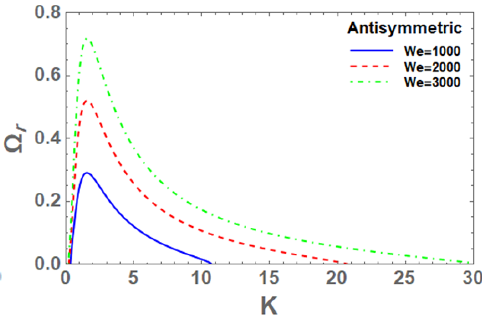
8.1. Effect of the Weber Number

For various values of the Weber number and constant values of other parameters included in the analysis, the non-dimensional growth rate ${\Omega }_r$ is shown in Figure 3 for the antisymmetric disturbance example. This graph shows that when the Weber number rises, so do the dominant growth rates, dominant wave numbers, and critical wave numbers. Consequently, the instability zone expands, demonstrating that the Weber number destabilizes the system.

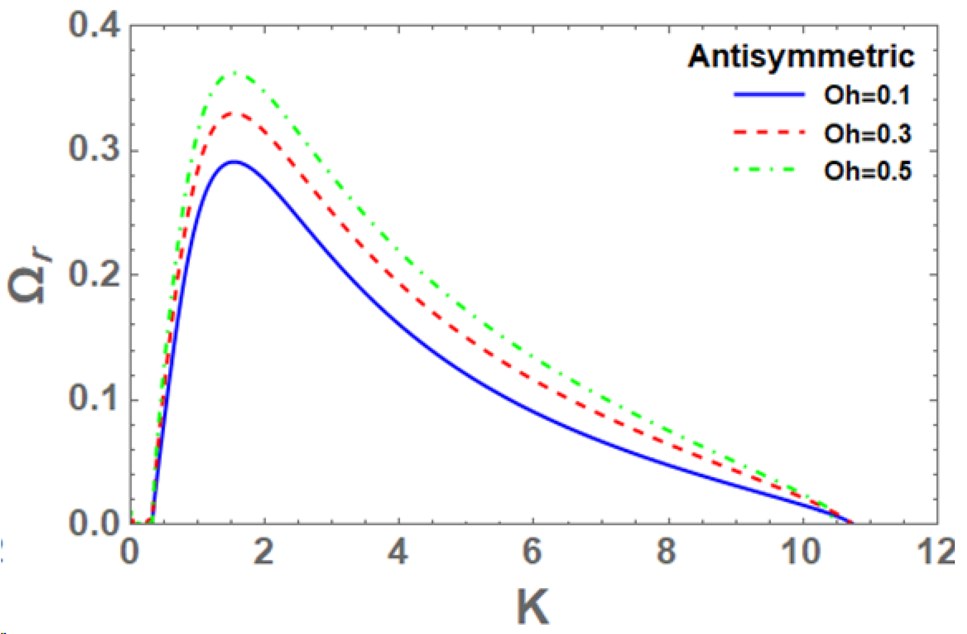
8.2. Effect of Ohnesorge Number

For antisymmetric disturbances with fixed physical parameters, the Ohnesorge number $Oh$ affects the non-dimensional growth rate ${\Omega }_r$ against the non-dimensional wave number K in Figure 4. The figure shows that all curves have the same wave number at both the beginning and the conclusion, as can be seen. Increasing the Ohnesorge number $Oh$ raises the maximum dominant wave numbers, and they are the same as the dominant wave number, while the critical wave numbers remain unchanged. As a result, we can infer that the Ohnesorge number $Oh$ destabilizes the system under consideration as the unstable zone under the curves expands.

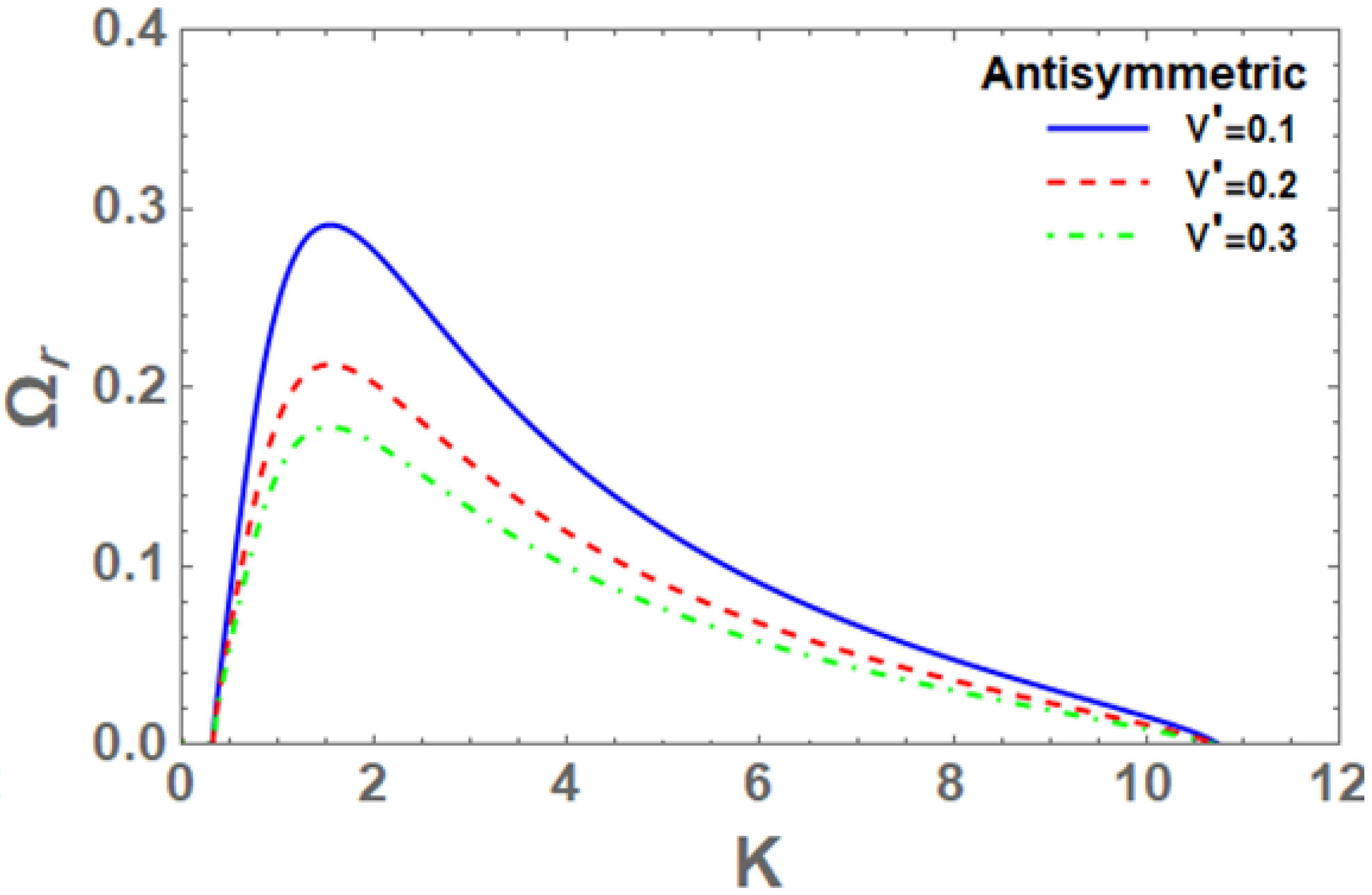
8.3. Effect of Viscolasticity Parameter

Viscoelasticity parameter and other physical constants remain constant in the antisymmetric disturbance situation, hence the growth rate ${\Omega }_r$ of the non-dimensional wave number K is shown in Figure 5. The graphic shows that the maximum dominating growth rates fall as the viscoelasticity parameter $V^{\prime }$ is increased, and that all curves have the same starting wave number value and critical wave number value. The instability zone shrinks when the viscoelasticity parameter $V^{\prime }$ is increased, indicating that the viscoelasticity parameter $V^{\prime }$ has a stabilizing effect.

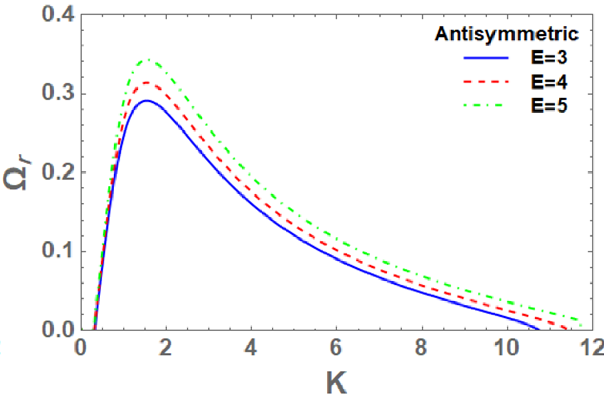
8.4. Effect of Electric Field

According to the antisymmetric disturbance case, the relationship between non-dimensional growth rate ${\Omega }_r$ and non-dimensional wave number K can be seen in Figure 5 for various electric field E values and constant other physical parameters. Increasing the electric field E values increases both the maximum dominant wave numbers and critical wave numbers, but the dominant wave number remains constant. For this sort of disturbance, the electric field has a destabilizing effect because it increases the instability zones.

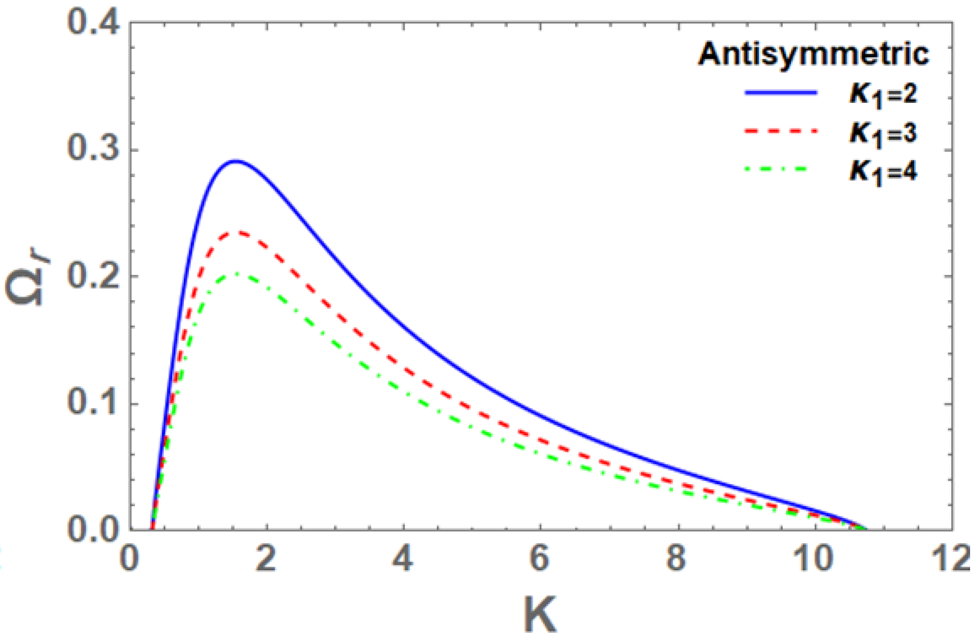
8.5. Effect of Medium Permeability

The antisymmetric disturbance mode is depicted in Figure 7, which shows how disturbance ${\Omega }_r$ growth rate changes with non-dimensional wave number K under various values of medium permeability ${\kappa }_1$ and constant values of other physical parameters. For example, we see in this figure that as permeability is increased, dominant and critical wave numbers remain at their predetermined values due to lower maximum dominant growth rates. Increased values of medium permeability ${\kappa }_1$, therefore, we suggest that medium permeability has stabilizing effects on this system of interest.

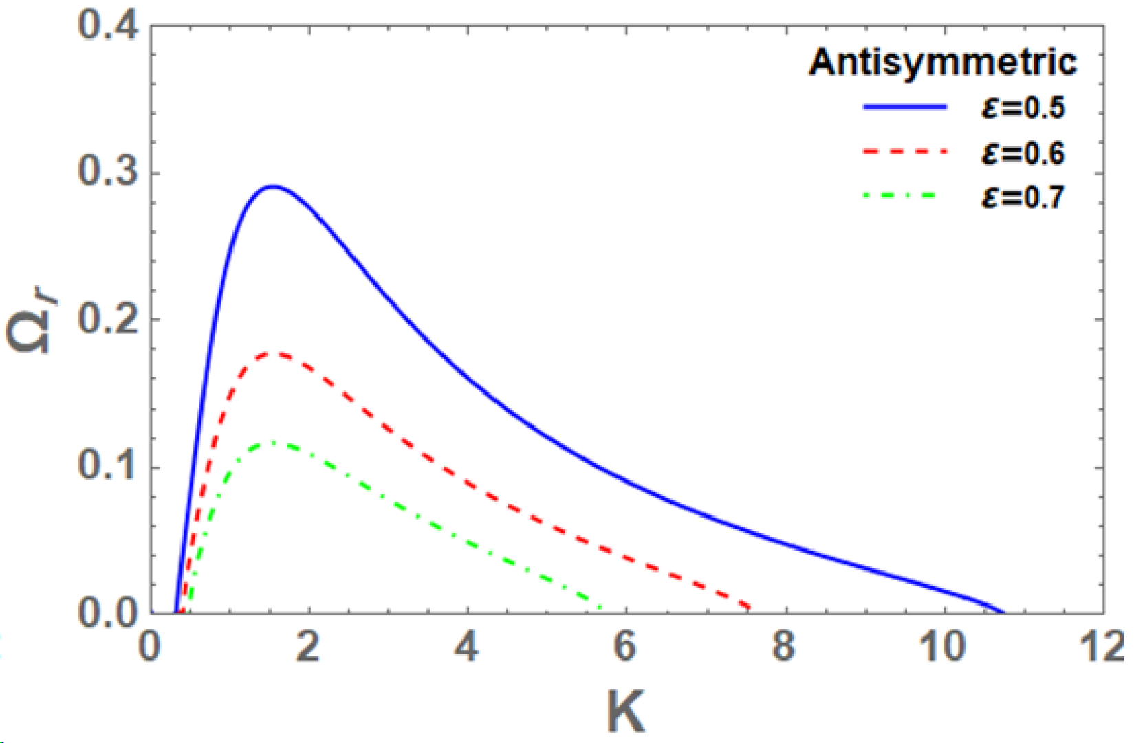
8.6. Effect of Porosity of Porous Medium

Using a non-dimensional growth rate ${\Omega }_r$ vs. a non-dimensional wave number K and the same values for the other parameters, Figure 8 depicts the effect of porous medium $\epsilon$ porosity on the instability of couple-stress viscoelastic electrified liquid sheets for antisymmetric disturbances. Increasing the porosity of porous medium decreases the maximum dominant growth rate ${\Omega }_r$, but they retain at the same dominent wave number value. As a result, we may deduce that increasing the porosity of a porous medium $\epsilon$ stabilizes this system by raising the starting wave numbers and critical wave numbers, respectively, while decreasing the instability zones.

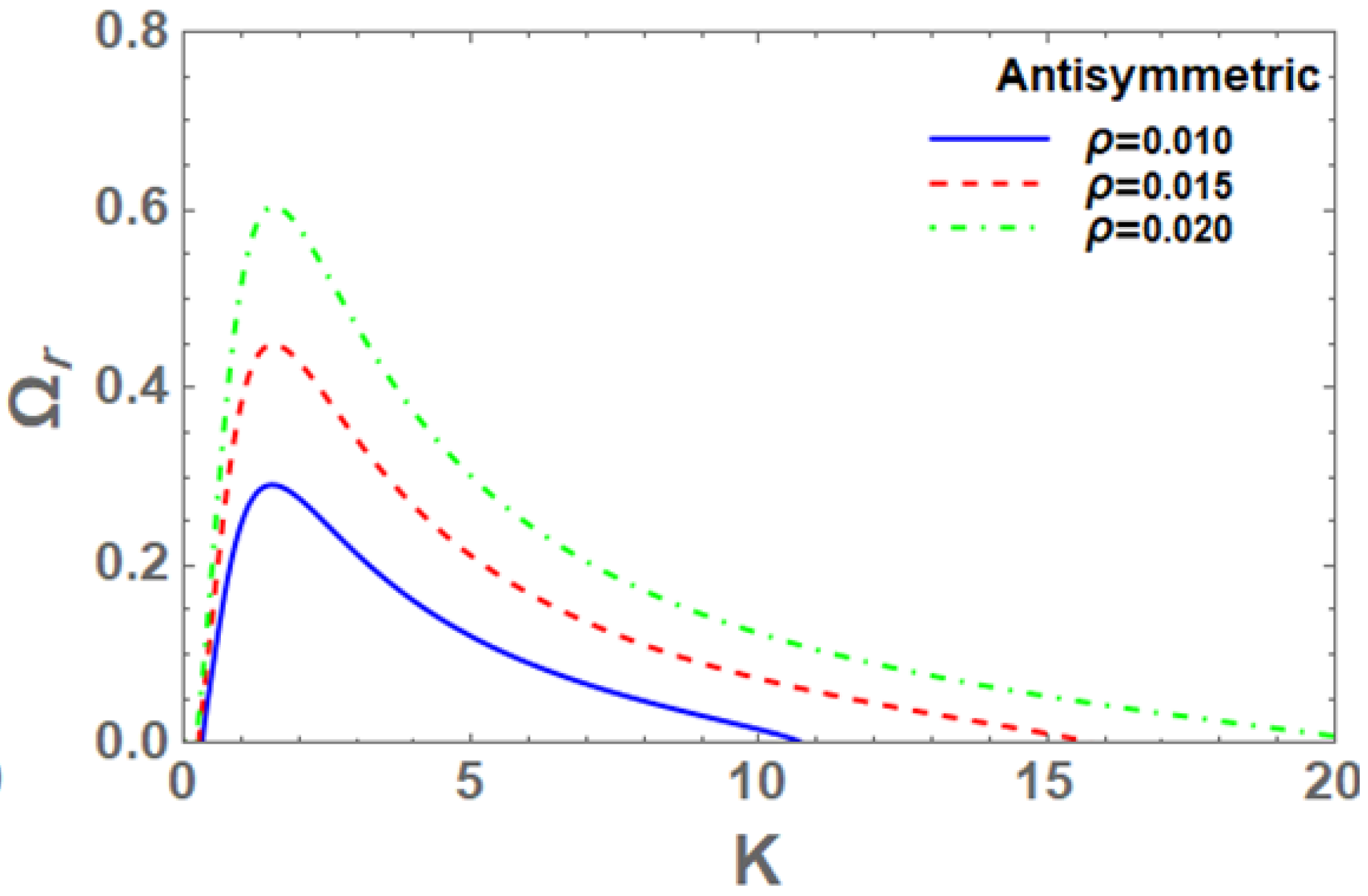
8.7. Effect of Gas to Liquid Density Ratio

Non-dimensional growth rate of disturbance ${\Omega }_r$ with non-dimensional wave number K for varying gas to liquid density ratio $\rho$ and constant values of the other physical parameters is shown in Figure 9 for antisymmetric disturbance modes. When the gas to liquid density ratio grows, both the dominant growth rates and crucial wave numbers increase, while the dominant wave numbers occur at the same fixed wave number value and the starting points of the curves are coincidental. The instability zone expands as the gas-to-liquid density ratio increases, demonstrating the destabilizing effect of gas to liquid density on the examined structure.

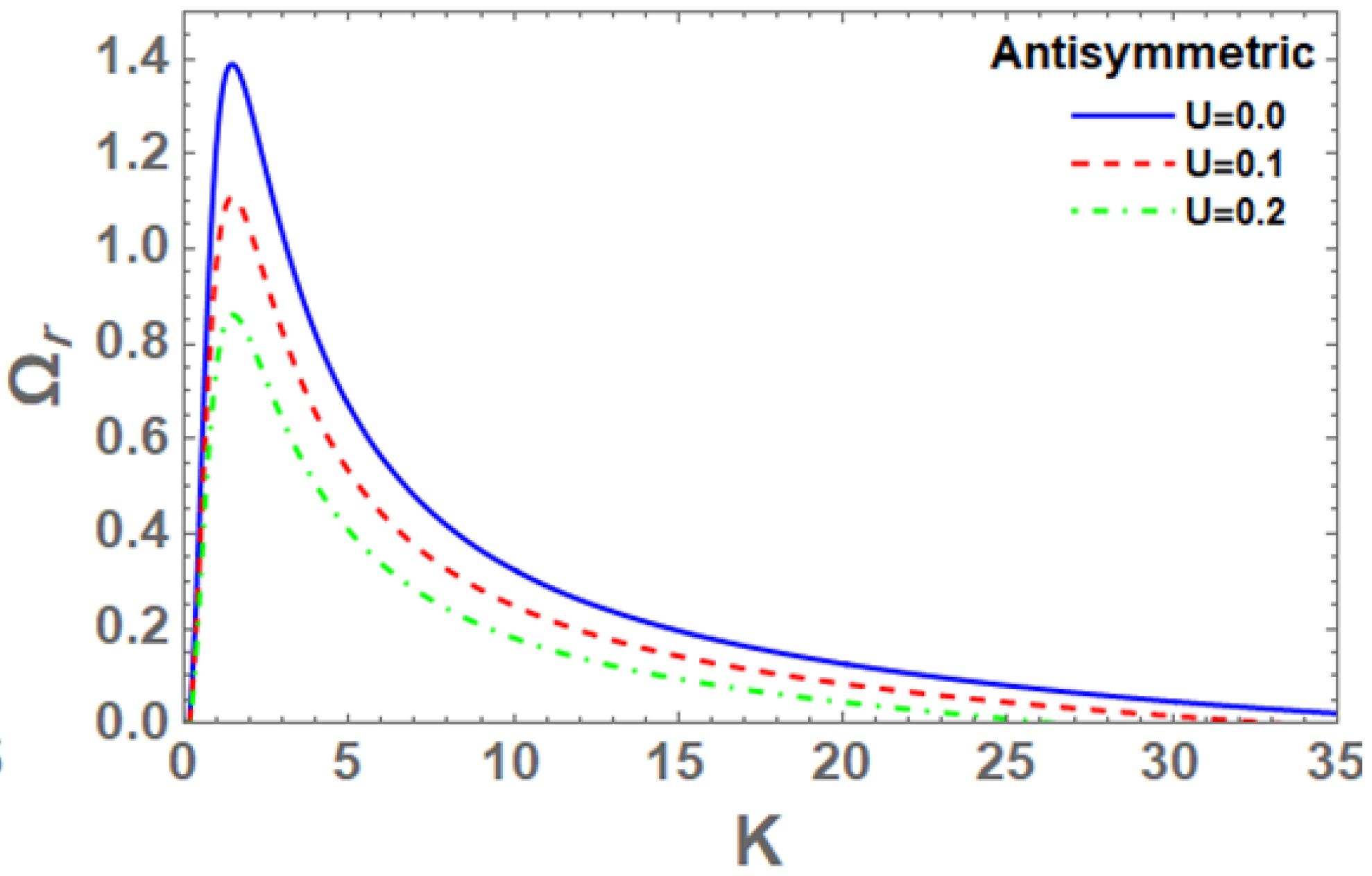
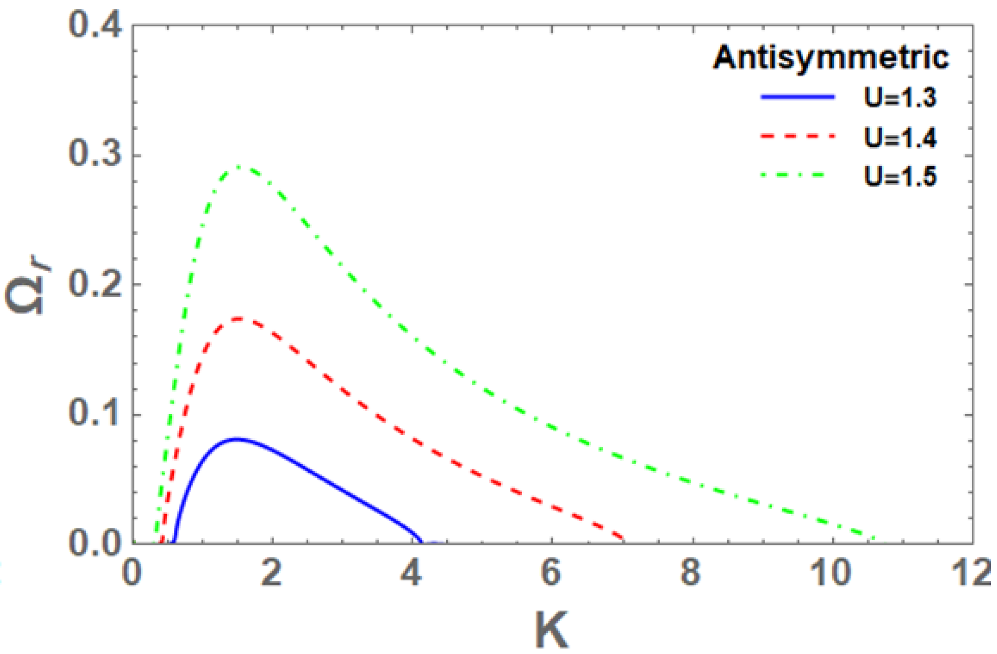
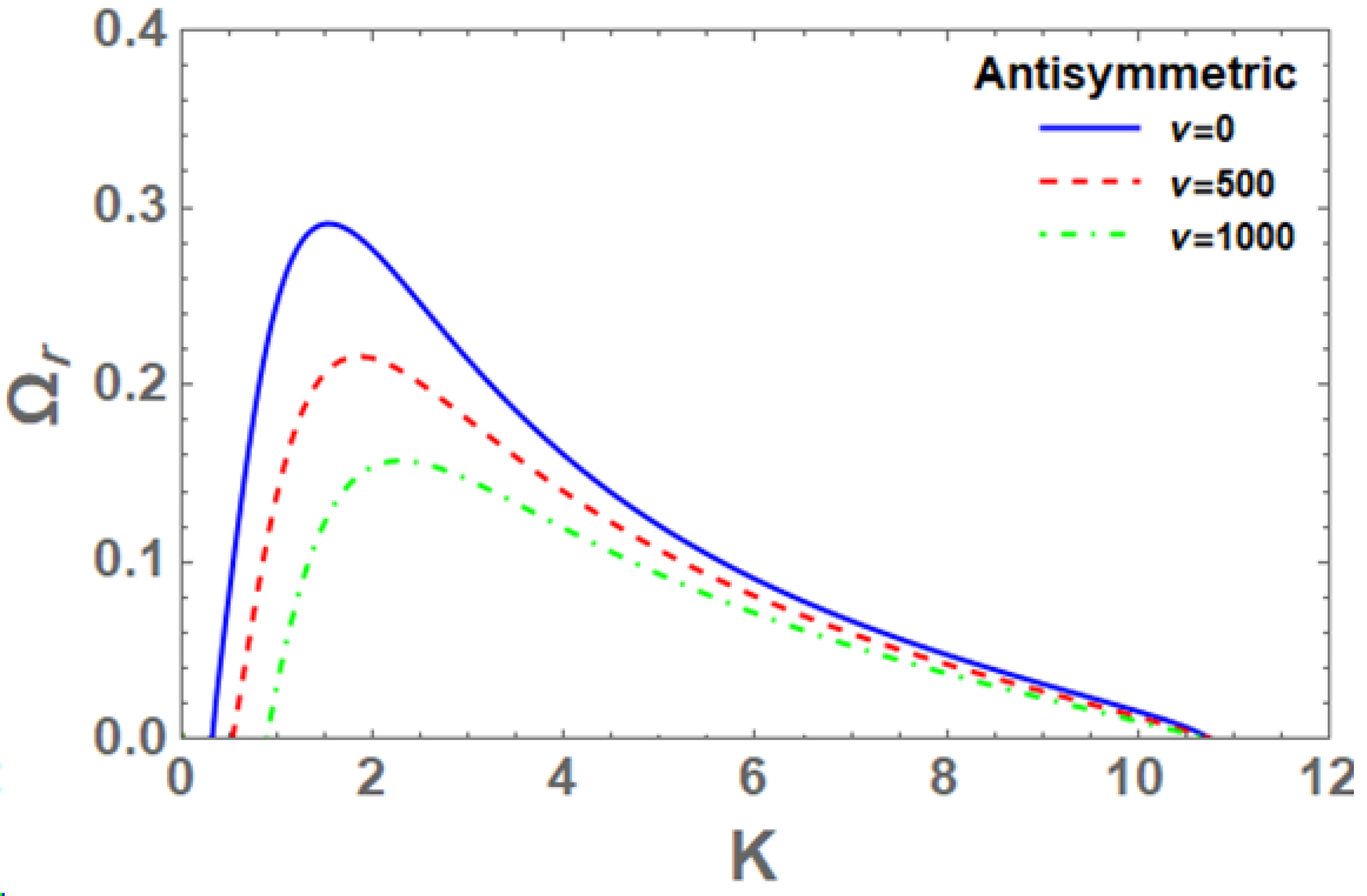
8.8. Effect of Gas to Liquid Velocity Ratio

There is an antisymmetric form of disturbance when U≶ 1, which is depicted in Figure 10 and Figure 11 by the fluctuation of the non-dimensional growth rate ${\Omega }_r$ with the non-dimensional wave number K for various values of the gas to liquid velocity ratio U. With increasing gas to liquid velocity ratio U < 1, both dominating growth rates and critical wave numbers drop, and thus the instability zone reduces as well, as seen in Figure 10. Therefore, we infer that the gas to liquid velocity ratio $0\le U<$ 1 stabilizes the system in question, as seen in the following figure: As shown in Figure 11, the gas to liquid velocity ratio greater than one ($U>$ 1) has a destabilizing effect on a similar system. Furthermore, keep in mind that the dominant wave numbers fall and grow (slightly) as the gas to liquid velocity ratio increases in the cases when U≶ 1. Therefore, we conclude that the ratio of gas to liquid velocity affects the stability of the system in two ways. Stabilization and destabilization of the system are both dependent on U ≶ 1, and vice versa.

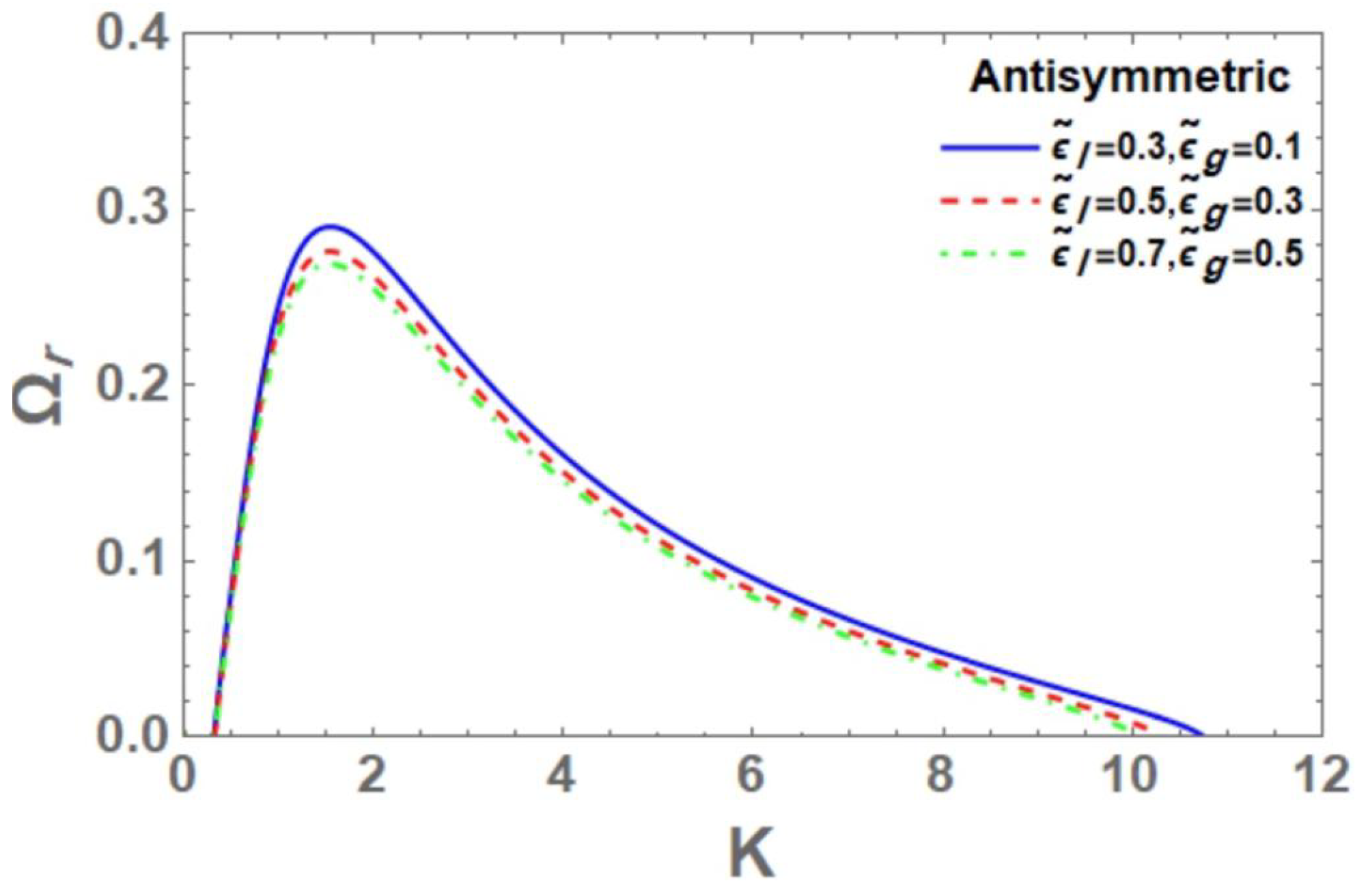
8.9. Effect of Dielectric Constants

Non-dimensional growth rate ${\Omega }_r$ is shown in relation to the now-dimensional wave number K for different values of dielectric constant ${\widetilde{ϵ}}_l,{\widetilde{ϵ}}_g$ in liquid and gaseous media. As dielectric constants are increased, the resultant curves tend to converge and the instability zones narrow gradually, as seen by the curves’ behavior. The dislectric constants ${\widetilde{ϵ}}_l,{\widetilde{ϵ}}_g$ in liquid and gas media have a small stabilizing influence on the system under consideration, therefore we can draw this conclusion.

8.10. Effect of Gas to Liquid Viscosity Ratio

Figure 13 shows the non-dimensional growth rate ${\Omega }_r$ vs. the non-dimensional wave number K as a function of the gas to liquid viscosity ratio $\nu$ and various other factors. The figure clearly shows that the system is stable in the absence of gas viscosity, and we found that increasing the gas to liquid viscosity ratio $\nu$ caused all of the curves to nearly coincide, but the figure is not shown here. This result shows that the system is neutrally unstable for small values of the gas to liquid viscosity ratio. It is also worth noting that the maximum dominant growth rates and, thus, the instability zones shrink when the gas to liquid viscosity ratio rises significantly. For very low gas to liquid viscosity ratios, the corresponding effect is only mildly stabilizing, but for high gas to liquid viscosity ratios, the effect is stabilizing.

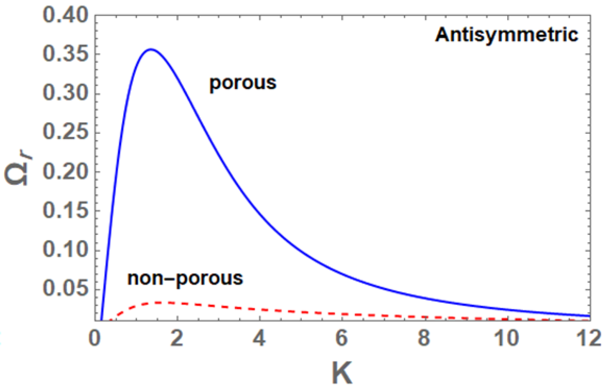
8.11. Effect of Porous Medium

As shown in Figure 14, for antisymmetric disturbance mode, the non-dimensional growth rate ${\Omega }_r$ and wave number K are related to each other in the presence ($\epsilon$ and ${\kappa }_1$) and absence ($\epsilon =1$ and ${\kappa }_1\to$∞ ) of porous media. The presence of porous media makes the system more unstable than it would be in the absence of porous medium, as can be seen from this image. All preceding figures that indicate the effect of other parameters, such as Figure 7 and Figure 8, are based on this result. As a result, we have come to the conclusion that the system is more susceptible to breakup in the presence of porous medium than in the absence of such media.

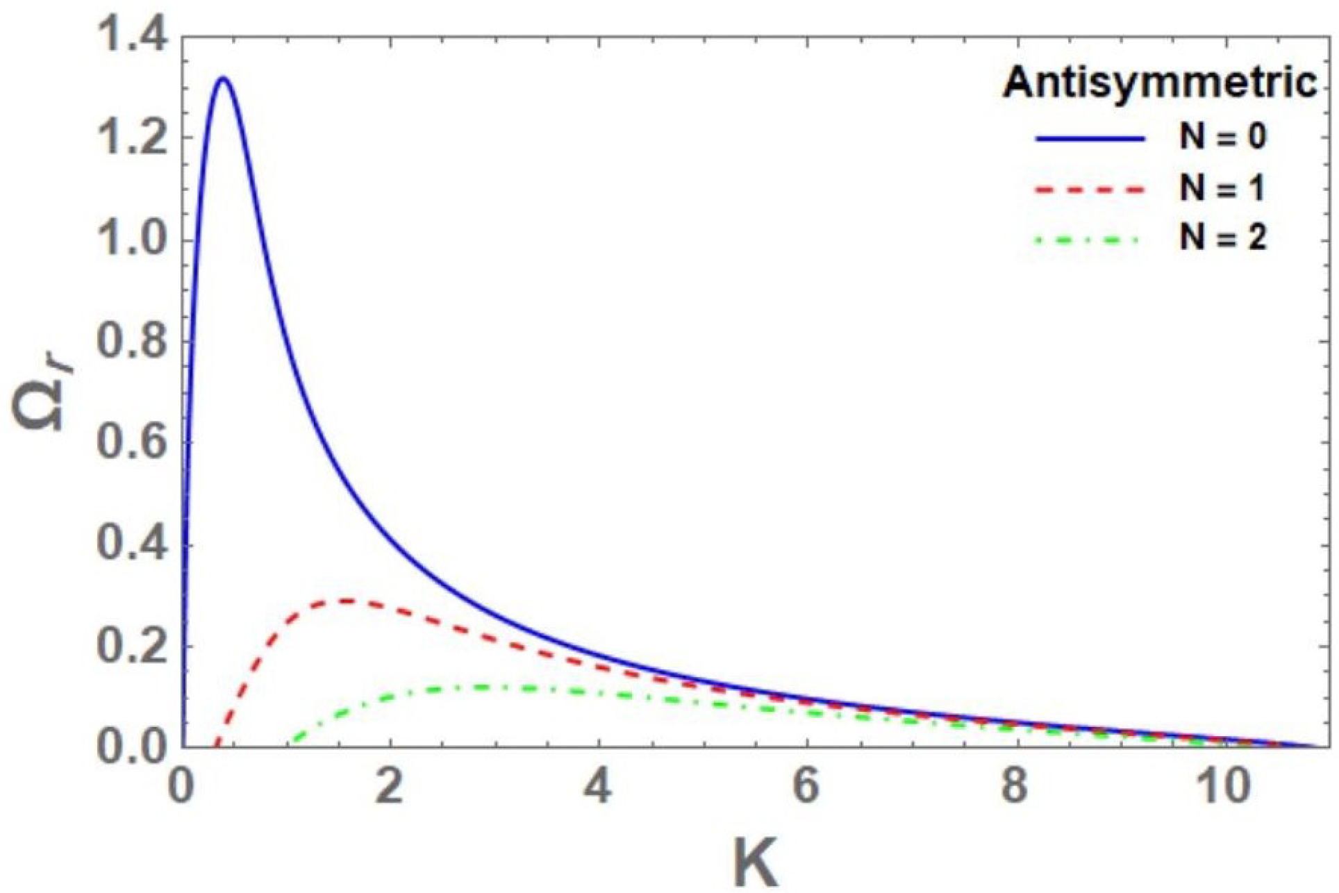
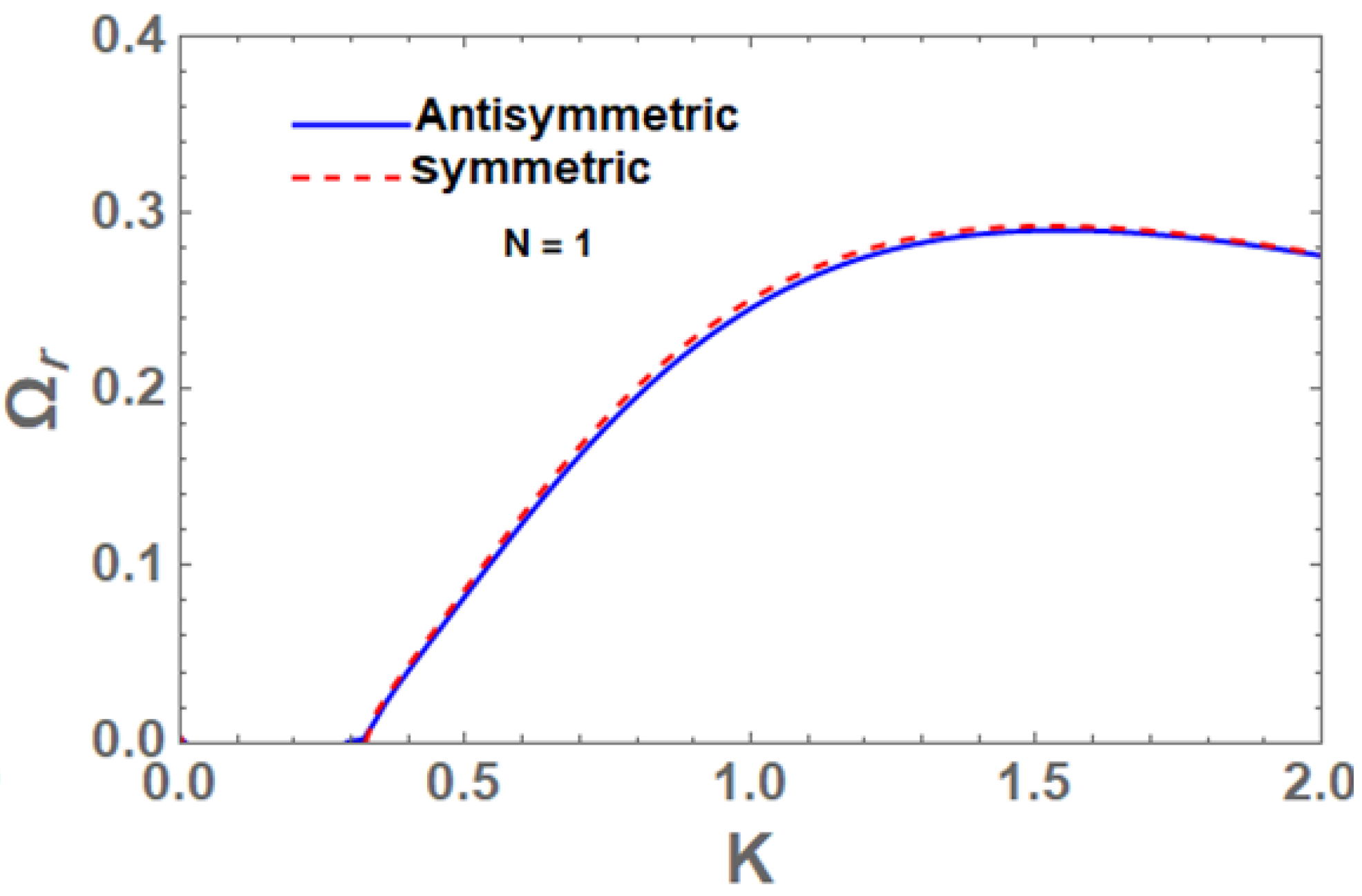
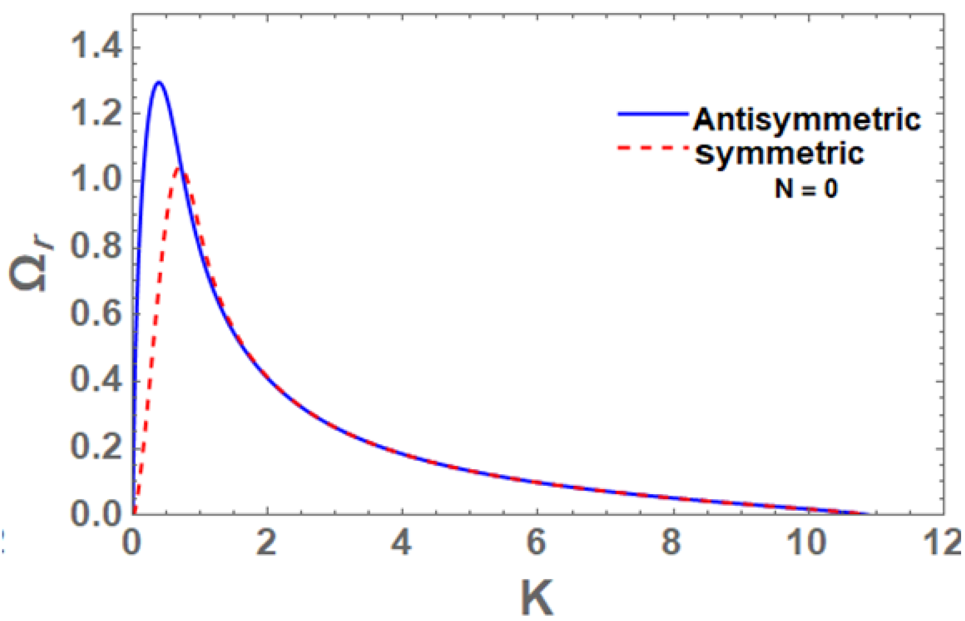
8.12. Effect of Dimension

There is an inverse relationship between non-dimensional growth rates ${\Omega }_r$ and non-dimensional wave number K in the cases of a three-dimensional configuration $(N=1)$ and a zero dimension $(N=0)$, as shown in Figure 15 and Figure 16. According to Figure 15, both symmetric and antisymmetric disturbances have nearly the same influence on the increasing rate of instability in the three-dimensional example. There is no difference between an antisymmetric or symmetric disturbance’s impact on instability, because the growth rate curves are nearly identical. Figure 16 shows that for small wave numbers, the dominating growth rate for antisymmetric disturbance mode is higher than the equivalent symmetric disturbance mode, whereas for higher wave numbers, the growth rate curves for both antisymmetric and symmetric cases are coincident. To sum up, in the three-dimensional disturbance case, every parameter has an identical effect in both antisymmetric and symmetric mods, but in the two-dimensional disturbance case, the antisymmetric instability zone is larger than the symmetric instability zone, and as a result, the system is more unstable when configured in the antisymmetric mode than when configured in the symmetric mode.

9. Concluding Remarks

An incompressible viscoelastic dielectric liquid sheet of the couple-stress type streaming with relative velocity in an inviscid dielectric gas medium through a porous medium has been studied using fluid and electric field equations of motion with the corresponding appropriate boundary conditions in this work, resulting in an electrohydrodynamic instability analysis. It was found that there are two types of disturbances: antisymmetric and symmetrical. Analytically, we may derive the dispersion relations for both antisymmetric and symmetric disturbances, and by defining some non-dimensional qualities of the parameters included in our analysis, we can represent the derived dispersion equations in dimensionless forms. The influence of various factors on the instability of this type of liquid sheet problem can be explored by computationally resolving the non-dimensional dispersion relations using Mathematica software via the Gaster technique. Based on the preceding discussion and examination of the numbers, here are a few possible conclusions:

(1)

When a system is placed in a two-dimensional configuration, it is more unstable when it is subjected to antisymmetric disturbance than when it is subjected to symmetric disturbance.

(2)

A porous medium makes the system more unstable, and it breaks down more quickly, compared to the lack of a porous medium.

(3)

Ohnesorge number, Weber number, and electric field all have a destabilizing effect on the system under consideration.

(4)

The system is stabilized by the viscoelasticity parameter, the medium permeability, the porous medium porosity, and the gas to liquid viscosity ratio.

(5)

We have found that the dielectric constants have a small stabilizing effect.

(6)

The gas to liquid velocity ratio affects system stability in two ways: it stabilizes when $U<1$ is less than one, and it destabilizes when $U>1$ is more than one.

References

1. Squire, H.B. Investigation of the instability of a moving liquid Sheet. Br. J. Appl. Phys. 1953, 4, 167–169. [Google Scholar] [CrossRef]
2. Hagerty, W.W.; Shea, J.F. A study of the stability of plane fluid sheets. J. Appl. Mech. 1955, 22, 509–514. [Google Scholar] [CrossRef]
3. Dombrowski, N.; Johns, W.R. The aerodynamic instability and disintegration of viscous liquid sheets. Chem. Eng. Sci. 1963, 18, 203–214. [Google Scholar] [CrossRef]
4. Li, X.; Tankin, R.S. On the temporal instability of a two-dimensional viscous liquid sheet. J. Fluid Mech. 1991, 225, 425–443. [Google Scholar] [CrossRef]
5. Tong, M.-X.; Fu, Q.-F.; Yang, L.-J. Two-dimensional instability responce of an electrified viscoelastic planar liquid sheet subjected to unrelaxed axial elastic tension. At. Sprays 2015, 25, 99–121. [Google Scholar] [CrossRef]
6. Lefebvre, A.H. Atomization and Sprays; Hemisphere: New York, NY, USA, 1989. [Google Scholar]
7. Yarin, A.L. Free Liquid Jets Films: Hydrodynamics and Rheology; John Wiley & Sons: New York, NY, USA, 1993. [Google Scholar]
8. Lin, S.P. Breakup of Liquid Sheets and Jets, 2nd ed.; Cambridge University Press: New York, NY, USA, 2010. [Google Scholar]
9. Dasgupta, D.; Nath, S.; Makhopadhyay, A. Linear and nonlinear analysis of breakup of liquid sheats: A Review. J. Indian Inst. Sci. 2019, 99, 59–75. [Google Scholar] [CrossRef]
10. Liu, Z.; Braen, G.; Durst, F. Linear analysis of the instability of two-dimensional non-Newtonian liquid sheets. J. Non–Newton. Fluid Mach. 1998, 78, 133–166. [Google Scholar] [CrossRef]
11. Brenn, G.; Liu, Z.; Durst, F. Three dimensional temporal instability of non- Newtonian liquid sheets. At. Sprays 2001, 11, 49–84. [Google Scholar] [CrossRef]
12. Yang, L.-J.; Liu, Y.-X.; Fu, Q.-F.; Wang, C.; Ning, Y. Linear stability analysis of electrified viscoelastic liquid sheets. At. Sprays 2012, 22, 951–982. [Google Scholar] [CrossRef]
13. El-Sayed, M.F.; Moatimid, G.M.; Elsabaa, F.M.F.; Amer, M.F.E. Electrohydrodynamic instability of non-Newtonian dielectric liquid sheet issued into streaming dielectric gaseous environment. Interfacial Phenom. Heat Transf. 2015, 3, 159–183. [Google Scholar] [CrossRef]
14. Melcher, J.R. Continuum Electromechanics; MIT Press: Cambridge, MA, USA, 1981. [Google Scholar]
15. Stokes, V.K. Couple stresses in fluids. Phys. Fluids 1966, 9, 1709–1715. [Google Scholar] [CrossRef]
16. Chavaraddi, K.B.; Awati, V.B.; Gouder, P.M. Effects of boundary roughness on Rayleigh-Taylor instability of a couple-stress fluid. Gen. Math. Notes 2013, 17, 66–75. [Google Scholar]
17. Chavaraddi, K.B.; Katagi, N.N.; Awati, V.B.; Gouder, P.M. Effect of boundary roughness on Kelvin-Helmholtz instability in couple stress fluid layer bounded above by a porous layer and below by rigid surface. Int. J. Chem. Eng. Res. 2014, 4, 35–43. [Google Scholar]
18. Chavaraddi, K.B.; Gouder, P.M.; Kudenatti, R.B. The influence of boundary roughness on Rayleigh-Taylor instability at the interface of superposed couple-stress fluids. J. Adv. Res. Fluid Mech. Thermal Sci. 2020, 75, 1–10. [Google Scholar] [CrossRef]
19. Rudrauah, R.; Chandrashekara, G. Effects of couple stress on the growth rate of Rayleigh-Taylor instability at the interface in a finite thickness couple stress fluid. J. Appl. Fluid Mech. 2010, 3, 83–89. [Google Scholar]
20. Sharma, R.C.; Sunil; Sharma, Y.D.; Chandel, R.S. On couple-stress fluid permeated with suspended particles heated from below. Arch. Mech. 2002, 54, 287–298. [Google Scholar]
21. Kumar, P.; Lal, R.; Sharma, P. Effect of rotation on thermal instability in couple-stress elastic-viscous fluid. Z. Naturforsh. A 2004, 59, 407–4011. [Google Scholar] [CrossRef]
22. Kumar, P.; Sing, G.J. Analysis of stability in couple-stress magneto-fluid. Nepal J. Math. Sci. 2021, 2, 35–42. [Google Scholar] [CrossRef]
23. Nield, D.A.; Bejan, A. Convection in Porous Medium, 3rd ed.; Springer: New York, NY, USA, 2006. [Google Scholar]
24. Mathur, R.P.; Gupta, D. Effect of surface tension on the stability of superposed viscous-viscoelastic (couple-stress) fluids through porous medium. Proc. Indian Natn. Sci. Acad. 2011, 77, 335–342. [Google Scholar]
25. Shankar, B.M.; Shivakumara, I.S.; Ng, C.O. Stability of couple stress fluid flow through a horizontal porous layer. J. Porous Med. 2016, 19, 391–404. [Google Scholar] [CrossRef]
26. Rudraiah, N.; Shankar, B.M. Stability of Parallel couple strep viscous fluid flow in a channel. Int. J. Appl. Math. 2009, 1, 67–78. [Google Scholar]
27. Agoor, M.B.; Eldabe, N.T.M. Rayleigh-Taylor instability at the interface of superposed couple-stress casson fluids flow in porous medium under the effect of a magnetic field. J. Appl. Fluid. Mech. 2014, 7, 573–580. [Google Scholar]
28. Shirakumara, I.S.; Kumar, S.S.; Devaraju, N. Effect of non- uniform Temperature gradients on the onset of convection in couple stress fluid-saturated porous medium. J. Appl. Fluid Mech. 2012, 5, 49–55. [Google Scholar]
29. Sharma, R.C.; Sunil Pal, M. On superposed couple-stress fluid in porous medium. Studia Geotech. Mech. 2001, 33, 55–66. [Google Scholar]
30. Rana, G.C.; Saxena, H.; Gautam, P.K. The onset of electrohydrodynamic instability in a couple-stress nanofluid saturating a porous medium: Brinkman model. Rev. Cubana Fis. 2019, 36, 37–45. [Google Scholar] [CrossRef]
31. Rudrajah, N.; Shankar, B.M.; Ng, C.O. Electrohydrodynamic stability of couple stress fluid flow in a channel occupied by a porous medium. Spec. Top. Rev. Porous Media 2011, 2, 11–22. [Google Scholar] [CrossRef]
32. El-Sayed, M.F.; Eldabe, N.T.; Haroun, M.H.; Mastafa, D.M. Nonlinear electroviscous potential flow instability of two superposed couple-stress fluids streaming through porous medium. J. Porous Med. 2014, 17, 405–420. [Google Scholar] [CrossRef]
33. Chandrasekhar, S. Hydrodynamic and Hydromagnetic Stability; Dover Publications: New York, NY, USA, 1981. [Google Scholar]
34. Shivakumara, I.S.; Akkanagamma, M.; Ng, C.-O. Electrohydrodynamic instability of a rotating couple-stress dielectric fluid layer. Int. J. Heat Mass Transfer. 2013, 62, 761–771. [Google Scholar] [CrossRef] [Green Version]
35. El-Sayed, M.F. Three-dimensional Electrohydrodynamic temporal instability of a moving dielectric liquid sheet emanated into a gas medium. Eur. Phys. J. E 2004, 15, 443–455. [Google Scholar] [CrossRef]
36. Ibrahim, E.A.; Akpan, E.T. Liquid sheat instability. Acta Mech. 1998, 131, 153–167. [Google Scholar] [CrossRef]
37. Dasgupta, D.; Nath, S.; Bhanja, D. Linear instability analysis of viscous planar liquid sheet sandwiched between two moving gas streams. In Advances in Mechanical Engineering; Lecture Notes in Mechanical Engineering; Biswal, B., Sarkar, B., Mahanta, P., Eds.; Springer: Singapore, 2020; pp. 41–50. [Google Scholar]
38. Nath, S.; Mukhopadhyay, A.; Sen, S.; Tharakan, T.J. Influence of gas velocity on breakup of planar liquid sheets sandwiched between two gas streams. At. Sprays 2010, 20, 983–1003. [Google Scholar] [CrossRef]
39. Gaster, M. A note on the relation between temporally increasing and spatially-increasing disturbances in hydrodynamic stability. J. Fluid Mech. 1962, 14, 222–224. [Google Scholar] [CrossRef]
40. El-Sayed, M.F.; Moatimid, G.M.; Elsabaa, F.M.F.; Amer, M.F.E. Axlaymmotric and asymmetric instabilities of a non-Nowtonian liquid jet moving in an Inviscid streaming gas through porous media. J. Porous Modia 2016, 19, 751–769. [Google Scholar] [CrossRef]
41. El-Sayed, M.F.; Moatimid, G.M.; Elsabaa, F.M.F.; Amer, M.F.E. Electrohydrodynamic instability of a non-Newtonian dielectric liquid jet moving in a streaming dielectric gas with a surface tension gradient. At. Sprays 2016, 26, 349–376. [Google Scholar] [CrossRef]
Figure 1. Description of the system for (a) Symmetric and (b) Antisymmetric disturbances.
Fluids 07 00247 g001
Figure 2. Variation in the non-dimensional growth rate Ω r with different values of the non-dimensional wave number K the two- and three-dimensional of configuration N = 0 and N = 1 , 2 , respectively, when W e = 1000; O h = 0.1; ρ = 0.01; v = 0.2; κ 1 = 2; ϵ ˜ l = 0.3; ϵ ˜ g = 0.1; E = 3; U = 1.5; V = 0.1; ε = 0.5, for axisymmetric disturbance case.
Fluids 07 00247 g002
Figure 3. For various Weber numbers W e , the variation in the non-dimensional growth rate Ω r depends on the non-dimensional wave number K, W e , when N = 1 ;   O h = 0.1 ;   ρ = 0.01 ;   n = 1 ;   v = 0.2 ;   κ 1 = 2 ;   ϵ ˜ l = 0.3 ;   ϵ ˜ g = 0.1 ;   E = 3 ;   U = 1.5 ; V = 0.1 ;   ε = 0.5 , for axisymmetric disturbance case.
Fluids 07 00247 g003
Figure 4. Non-dimensional growth rate Ω r and non-dimensional wave number K for different values of Ohnesorge number O h , when W e = 1000 ; N = 1 ; ρ = 0.01 ; v = 0.2 ; κ 1 = 2 ; ϵ ˜ l = 0.3 ; ϵ ˜ g = 0.1 ; E = 3 ; U = 1.5 ; V = 0.1 ; ε = 0.5 , for axisymmetric disturbance case.
Fluids 07 00247 g004
Figure 5. Non-dimensional growth rate Ω r and non-dimensional wave number K for different values of viscoelastitily parameter V , when W e = 1000 ;   O h = 0.1 ; ρ = 0.01 ; N = 1 ;   v = 0.2 ; κ 1 = 2 ;   ϵ ˜ l = 0.3 ;   ϵ ˜ g = 0.1 ;   U = 1.5 ;   ε = 0.5 , for axisymmetric disturbance case.
Fluids 07 00247 g005
Figure 6. Analysis of non-dimensional growth rate Ω r and non-dimensional wave number K for different electric field strengths E, when W e = 1000 ; Oh = 0.1 ;   ρ = 0.01 ;   N = 1 ; v = 0.2 ;   ϵ ˜ l = 0.3 ; ϵ ˜ g = 0.1 ;   E = 3 ; U = 1.5 ;   V = 0.1 ;   ε = 0.5 , for axisymmetric disturbance case.
Fluids 07 00247 g006
Figure 7. Variation of non-dimensional growth rate Ω r with non-dimensional wave number K for various medium permeability values κ 1 , when W e = 1000 ; Oh = 0.1 ;   ρ = 0.01 ; n = 1 ;   v = 0.2 ;   κ 1 = 2 ; ϵ ˜ l = 0.3 ;   ϵ ˜ g = 0.1 ;   E = 3 ; U = 1.5 ;   V = 0.1 , for axisymmetric disturbance case.
Fluids 07 00247 g007
Figure 8. Non-dimensional growth rate Ω r and non-dimensional wave number K for different values of porous medium porosity ε , when W e = 1000 ; O h = 0.1 ;   N = 1 ;   v = 0.2 ;   κ 1 = 2 ;   ϵ ˜ l = 0.3 ;   ϵ ˜ g = 0.1 ; E = 3 ; U = 1.5 ;   V = 0.1 ;   ε = 0.5 , for axisymmetric disturbance case.
Fluids 07 00247 g008
Figure 9. Non-dimensional growth rate Ω r and non-dimensional wave number K for different gas to liquid densities ρ , when W e = 1000 ; O h = 0.1 ;   N = 1 ; ρ = 0.01 ;   v = 0.2 ;   κ 1 = 2 ;   ϵ ˜ l = 0.3 ;   ϵ ˜ g = 0.1 ; E = 3 ; V = 0.1 ;   ε = 0.5 , for axisymmetric disturbance case.
Fluids 07 00247 g009
Figure 10. Change in non-dimensional growth rate Ω r with non-dimensional wave number K for varied gas to liquid velocity values U < 1 , when W e = 1000 ;   O h = 0.1 ;   N = 1 ; ρ = 0.01 ; v = 0.2 ;   κ 1 = 2 ; ϵ ˜ l = 0.3 ;   ϵ ˜ g = 0.1 ;   E = 3 ;   V = 0.1 ;   ε = 0.5 , for axisymmetric disturbance case.
Fluids 07 00247 g010
Figure 11. Variation of non-dimensional growth rate Ω r with non-dimensional wave number K for varied gas to liquid velocities U > 1 , when W e = 1000 ; Oh = 0.1 ;   N = 1 ; ρ = 0.01 ;   v = 0.2 ;   κ 1 = 2 ; E = 3 ;   V = 0.1 ;   ε = 0.5 , for axisymmetric disturbance case.
Fluids 07 00247 g011
Figure 12. Change in non-dimensional growth rate Ω r with non-dimensional wave number K for various dielectric constants values ϵ ˜ l and ϵ ˜ g , when W e = 1000 ;   O h = 0.1 ;   N = 1 ; ρ = 0.01 ;   κ 1 = 2 ; ϵ ˜ l = 0.3 ;   ϵ ˜ g = 0.1 ;   E = 3 ;   V = 0.1 ;   ε = 0.5 , for axisymmetric disturbance case.
Fluids 07 00247 g012
Figure 13. Non-dimensional growth rate Ω r and non-dimensional wave number K for different gas to liquid viscosity values ν , when W e = 2000 ; Oh = 2 ;   N = 1 ;   v = 0.2 ;   ρ = 0.1 ;   U = 1.5 ;   ϵ ˜ l = 0.3 ; ϵ ˜ g = 0.1 ; E = 10 ;   V = 5 ; for axisymmetric disturbance case.
Fluids 07 00247 g013
Figure 14. Non-dimensional growth rate Ω r and non-dimensional wave number K for both case of porous medium ε = 0.5 ;   κ 1 = 2 , and non-porous medium ε = 1 ;   κ 1 ), when W e = 2000 ; Oh = 2 ;   N = 1 ;   v = 0.2 ;   ρ = 0.1 ;   U = 1.5 ;   ϵ ˜ l = 0.3 ;   ϵ ˜ g = 0.1 ;   E = 10 ;   V = 5 ; for axisymmetric disturbance case.
Fluids 07 00247 g014
Figure 15. Variational of non-dimensional Ω r with non-dimensional K in three-dimensional case ( N = 1 ) for both anlisymmetric and symmetric disturbances with the same values of the parameters shown before.
Fluids 07 00247 g015
Figure 16. Change in in non-dimensional Ω r with non-dimensional K in two-dimensional case ( N = 0 ) for both antisymmetric and symmetric disturbances with the same values of the parameters used above.
Fluids 07 00247 g016
Publisher’s Note: MDPI stays neutral with regard to jurisdictional claims in published maps and institutional affiliations.