Article

Numerical Study of the Influence of the Critical Reynolds Number on the Aerodynamic Characteristics of the Wing Airfoil

1
Department of Applied Mathematics, Nizhny Novgorod State Technical University n.a. R.E. Alekseev, 24 ul. Minina, Nizhny Novgorod 603155, Russia
2
Russian Federal Nuclear Center All-Russian Research Institute of Experimental Physics FSUE RFNC—VNIIEF, Sarov, Mira Ave, 37, Nizhny Novgorod 607188, Russia
3
Aircraft Design and Certification Department, Moscow Aviation Institute, Volokolamskoe Shosse, 4, Moscow 125993, Russia
*
Author to whom correspondence should be addressed.
Submission received: 13 July 2023 / Revised: 27 September 2023 / Accepted: 28 September 2023 / Published: 13 October 2023

Abstract

:
The paper reports the results of a study concerned with the influence of the size of the leading edge laminar bubble on the aerodynamic characteristics of the HGR01 airfoil. The completely turbulent and transient flows are considered. The mechanism of the appearance and interaction of laminar and turbulent flow separation near the leading and trailing edges of the airfoil is studied in detail. In the paper, the dependence of aerodynamic forces on the critical Reynolds number for the HGR01 airfoil is discussed. It has been established that the separation bubble at the leading edge can only be obtained using the laminar–turbulent transition model. Fully turbulent models are not able to show this feature of the airfoil flow. Graphs of the lift coefficient as a function of the critical Reynolds number, as well as the pressure distribution as a function of the size of the laminar bubble, are shown.

1. Introduction

At a low angle of attack, the laminar boundary layer separates from the airfoil surface due to an unfavorable gradient in the middle part of the wing. In the detached flow, a laminar–turbulent transition occurs, and the turbulent flow reattaches to the airfoil surface. This local separation zone is called a “laminar separation bubble” [1]. One of the main goals of aircraft design is to maximize the wing lift coefficient. In practice, this leads to the need to take into account the separation of the laminar bubble from the leading edge, because it causes a hysteresis loop in the lift curve, which can be significant. The transition between positions on the curve can lead to a sharp loss of lift, and to prevent stall, a rapid change in the angle of attack is necessary. This was the reason for a detailed study of the occurrence and prevention of this phenomenon [1,2,3].
To calculate the maximum lift for airfoils with separation at the leading edge, it is important to accurately identify the separation point of the laminar bubble. Depending on the external conditions, the laminar bubble on the leading edge at large angles of attack can either “burst”, causing the so-called separation from the leading edge, or, for example, for higher critical Reynolds numbers, it can lead to a combination of separation from the leading and trailing edges, by interacting with the turbulent separation moving upstream from the trailing edge. In the latter case, the separation from the trailing edge may have a strong non-stationary character [1].
The study of the phenomenon is carried out experimentally by evaluating the position of the laminar bubble. It is clear that a comprehensive experimental study of this phenomenon is time-consuming and expensive; therefore, it is advisable to use mathematical modeling for the study, which has begun to be carried out in as yet isolated works. For example, at the Institute of Fluid Mechanics of Braunschweig Technical University, an investigation of the aerodynamic characteristics of the HGR01 airfoil [1] was carried out, purposely designed to study the separation of a mixed type (meaning the separation at both the leading and trailing edges).
It is shown in [1] that numerical modeling of the laminar–turbulent transition allows us to obtain a flow structure close to that observed in the experiment. In the case of modeling a laminar–turbulent transition, in contrast to modeling a fully developed turbulent flow, the result essentially depends on the critical Reynolds number, which is the function of turbulence intensity and pressure gradient.
The paper reports the results of the numerical simulation of the flow structure as affected by the critical Reynolds number. In the paper, the aerodynamic forces as a function of the critical Reynolds number for the HGR01 airfoil [1] are presented. The influence of the size of the leading-edge bubble on the aerodynamic characteristics of this airfoil is shown. The dependence of the lift coefficient on the critical Reynolds number, as well as the airfoil pressure distribution versus the size of the laminar bubble, are presented.

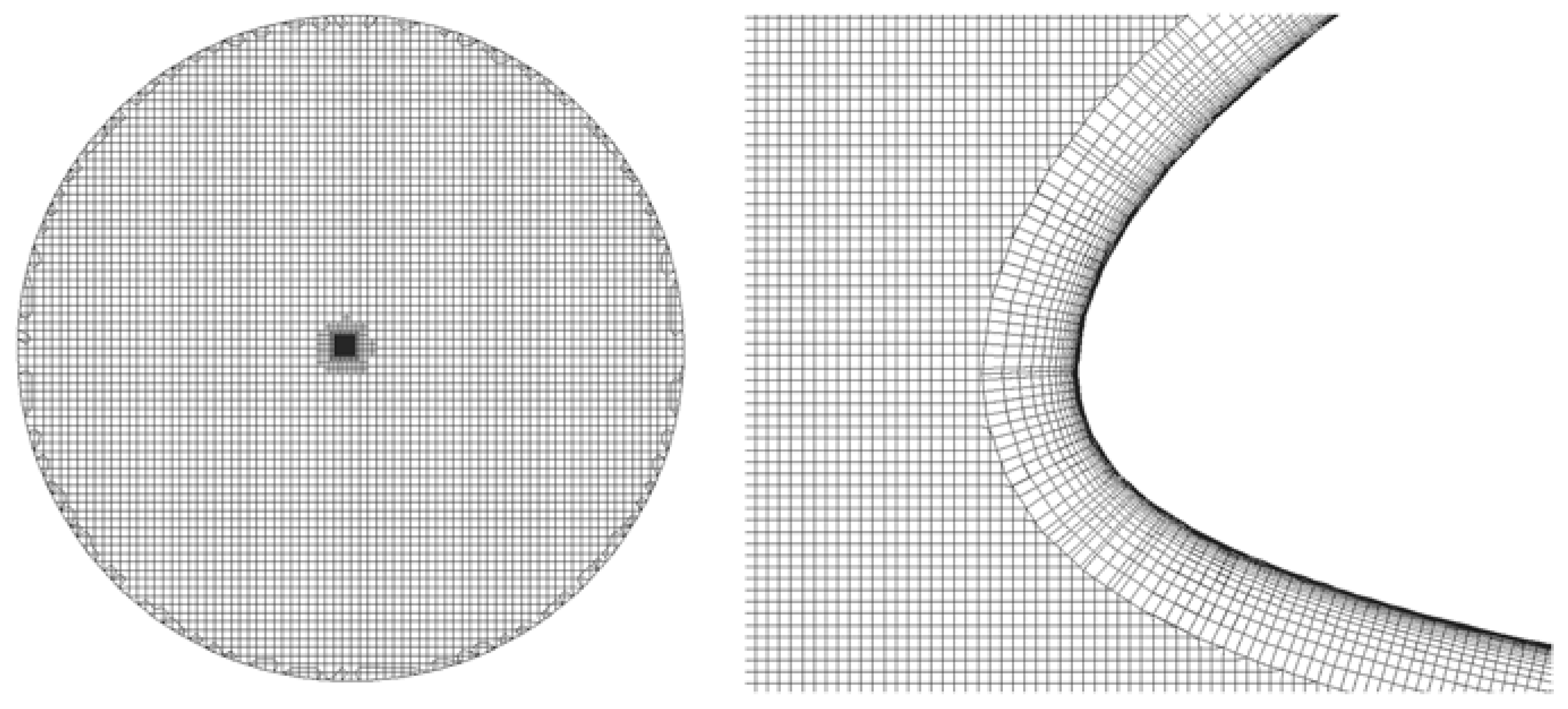
2. Model Implementation (Numerical Methods)

To study the influence of the position of the laminar bubble on the airfoil characteristics, we will use a well-known approach, based on the numerical solution of the Navier–Stokes equations averaged by Reynolds (RANS approach) [4]. In this approach, the one-parameter Spalart–Allmaras model (SA) [5] and the two-parameter Menter shear stress transport model (SST) [6] have been widely used. The disadvantage of the SA and SST models is the lack of correlation dependencies describing the laminar–turbulent transition. Therefore, these models cannot predict leading-edge laminar bubbles. Note that, although in the original Spalart–Allmaras model there is a term responsible for the laminar–turbulent transition, it requires an explicit assignment of the transition position.
To determine the position of the separation point, low-Reynolds number (low-Re) differential turbulence models were created. One of the most successful is the γ-Reθt model [7,8], developed with a focus on its use in conjunction with the SST turbulence model [6]. The γ-Reθt model uses a bypass transition scenario in which the transition to turbulence occurs in the region of linear stability of small perturbations. According to this scenario, the low-Re transition process begins with the sudden appearance of turbulent spots—the areas of turbulent pulsations, drifting downstream and increasing in size, lead to the complete turbulization of the downstream boundary layer. The formation of turbulent spots leads to the alternation of laminar and turbulent regimes in the boundary layer. This alternation can be characterized by the intermittency coefficient γ (the transition weight factor). The intermittency coefficient can be varied in order to artificially define laminar and turbulent flow regions.
The γ-Reθt model includes the transfer equation for the intermittency coefficient γ and the critical Reynolds number Reθt:
ρ γ t + ( ρ γ U j ) x j = P γ E γ + x j μ l + μ t σ γ γ x j
ρ Re θ t * t + ( ρ Re θ t * U j ) x j = P θ t + x j σ θ t μ l + μ t Re θ t * x j
where the terms of the equations take into account: P γ and E γ —the generation and dissipation of the intermittency γ; P θ t —the generation of the critical Reynolds number Reθt; and σ γ and σ θ t —the constants of the model. The term P γ is responsible for the transition onset and controls the length of the transition, and E γ is responsible for the suppression of γ in the laminar layer and in the viscous sublayer. The parameter Re θ t * is used to trigger the transition. The source term P θ t is responsible for the transfer Re θ t * so that the transferred scalar Re θ t * diffuses with the freestream flow. A complete description of the model with empirical relations is given in [8,9,10].
In the γ-Reθt turbulence model, the critical Reynolds number Re θ t * depends on a large number of calibration constants. In this paper, the γ-Reθt model, with an imposed critical Reynolds number, is used to control the length of the laminar portion of the boundary layer.
As will be shown below, classical RANS turbulence models do not allow description of the laminar separation bubble in the nose area at medium angles, which is consistent with the results of other studies [1,11]. To eliminate this disadvantage in RANS modeling, one can use the SSG/LRR-ω model, which better predicts the evolution of the boundary layer. A full description of the model can be found in [11]. Calculations were carried out with the LOGOS software package [12,13,14,15,16,17].

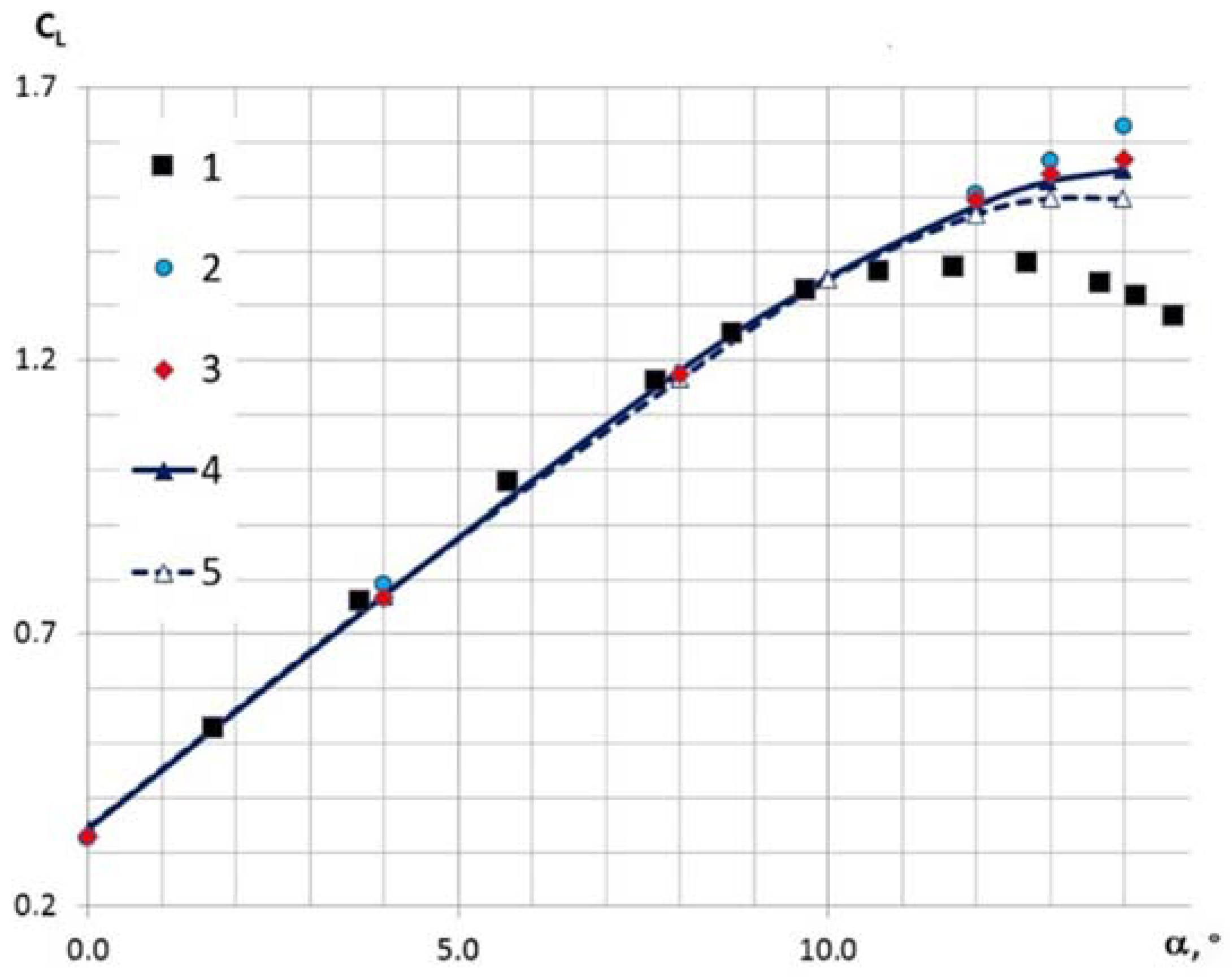
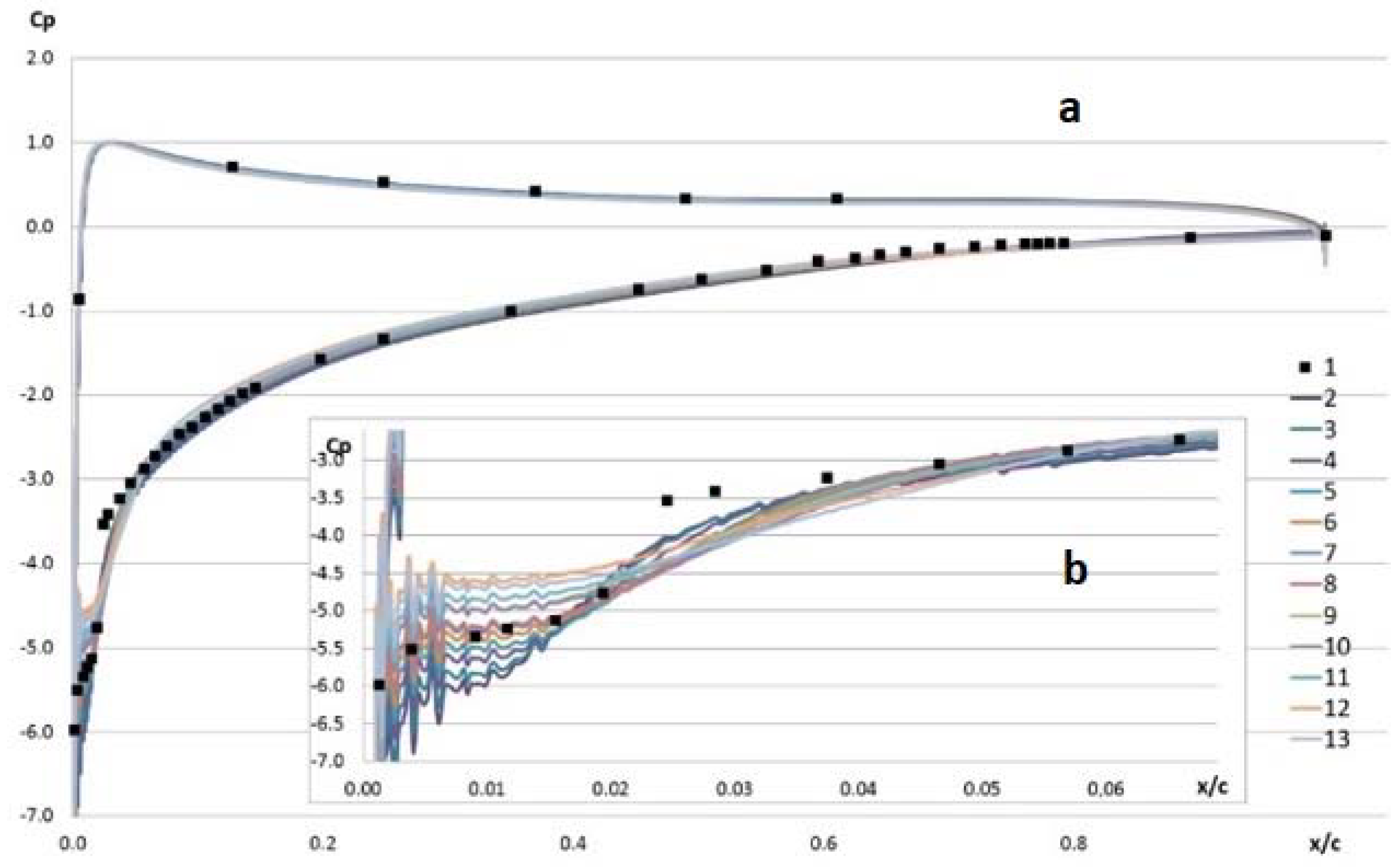
2.1. Predicting Lift Curve using RANS Turbulence Models

For the numerical experiment, an unstructured grid consisting of truncated hexagons and containing two million cells (Figure 1) was generated. The grid point nearest the wall has a distance to the wall of y+ ≈ 1. The case investigated here refers to the experiments carried out at a Mach number of M = 0 . 073 and a Reynolds number of Re = 0 . 65 × 10 6 . The boundaries of the computational domain were assigned to 100 reference lengths, so the turbulence parameters set at the inlet faded and had almost zero value near the airfoil, i.e., the incoming flow could be considered laminar.
A series of simulations using the turbulence models SSG/LRR-ω at different angles of attack was carried out. The results of calculations obtained by other authors are also given [11].
Figure 2 shows the corresponding lift curve. The graphs show the results of the experiment in [11], the numerical results obtained in Logos using the SA and RSM models, as well as others by the author of [11]. The experimental curve is close to linear, up to the angle of attack of 12°. Within the linear portion of the graph, there is a good agreement of the results for all turbulence models. The lift curves obtained using the turbulence model SA at angles of attack α ≥ 12°, retain a linear character. The results obtained using the RSM model show a deviation from linearity, but quantitatively they also differ significantly from the experimental data.
Figure 3 shows the streamlines at the airfoil trailing edge at α = 12°. Figure 3 demonstrates that in the experiment in [1], a bubble at the airfoil trailing edge is observed. The SSG/LRR-ω model shows the presence of only a small vortex zone, whereas, with the RANS turbulence models based on the Boussinesq hypothesis, no vortex is observed.
In the experiment with the HGR01 airfoil, a complex flow was recorded, including the leading-edge bubble. The bubble appeared at the average angles of attack long before there was turbulent separation from the trailing edge. Figure 4 shows the flow structure obtained in the experiment at an angle of attack of 10°. Figure 4 gives an example of the flow past the upper surface of the model visualized with oil paint. The extent of the separation bubble is clearly visible as a straight line of structured fluid film over the model span, as the paint is captured within the bubble through the experiment duration and is formed by surface tension and by flow structures within the bubble [1] (this is a quotation from [1]).
The reason for this is that under the considered conditions, the formation of a leading-edge laminar bubble is observed, which appears at the average angles of attack long before the trailing edge vortices [1]. As the angle of attack increases, the bubble shrinks and moves towards the leading edge. The presence of laminar flow on the leading edge leads to a decrease in friction force in this area.
Figure 5 shows the pressure coefficient distribution and the streamlines near the leading edge of the airfoil obtained with the RANS model.
It can be seen that with the RANS model, a flow circulation zone in the form of a laminar bubble is not formed at the leading edge. RANS turbulence models are based on a priori ideas about the nature of the flow, namely, fully developed turbulent flow. Therefore, no RANS model predicts the laminar boundary layer on the leading edge.

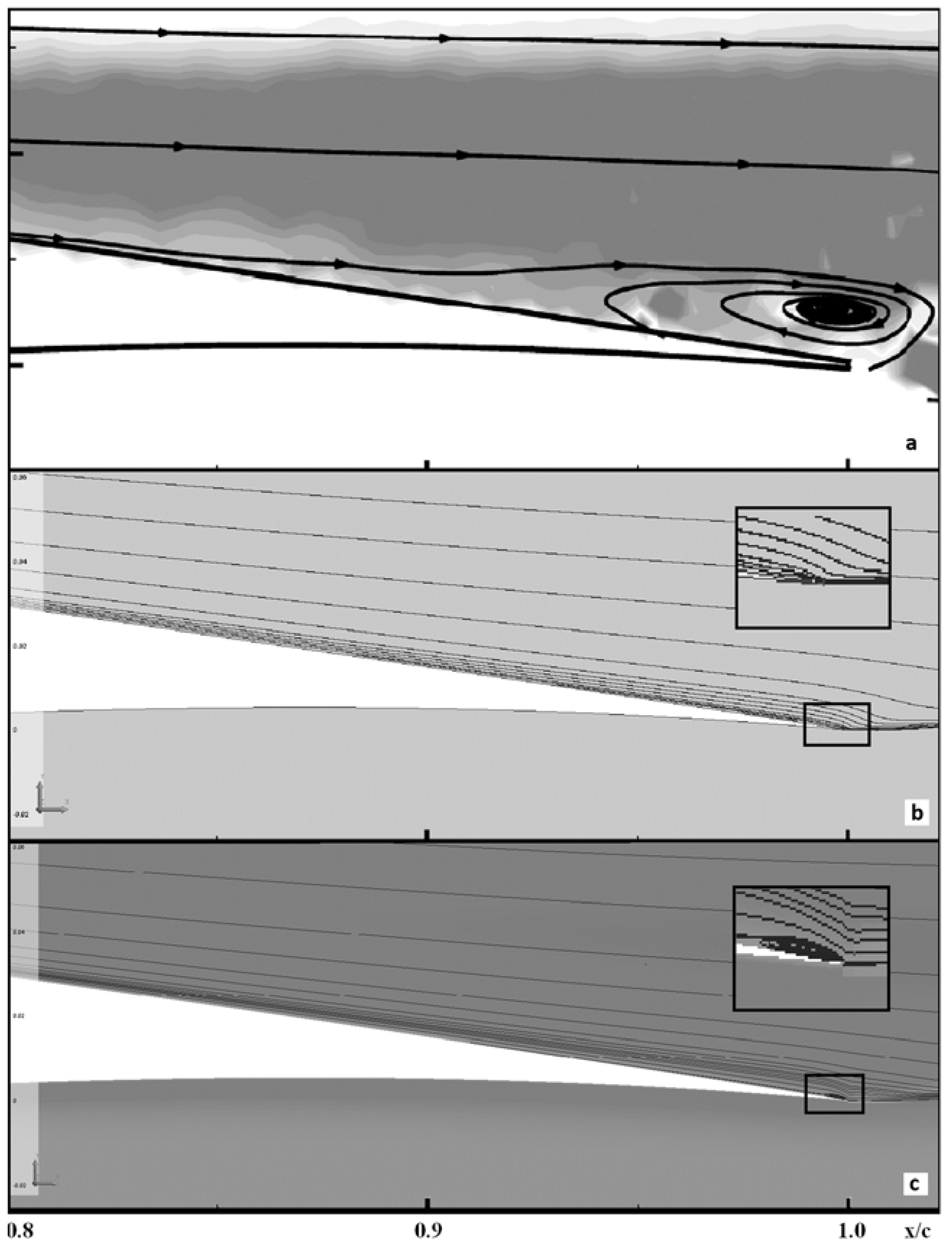
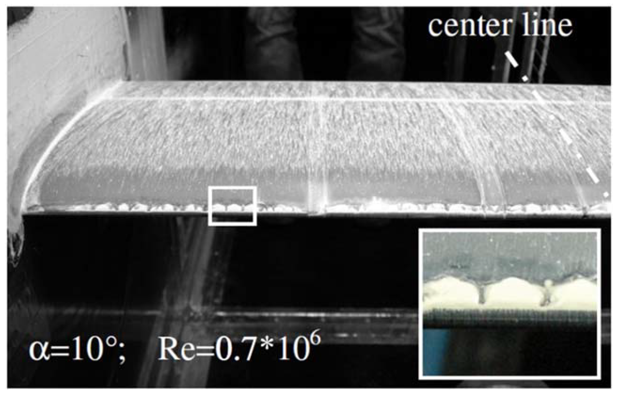
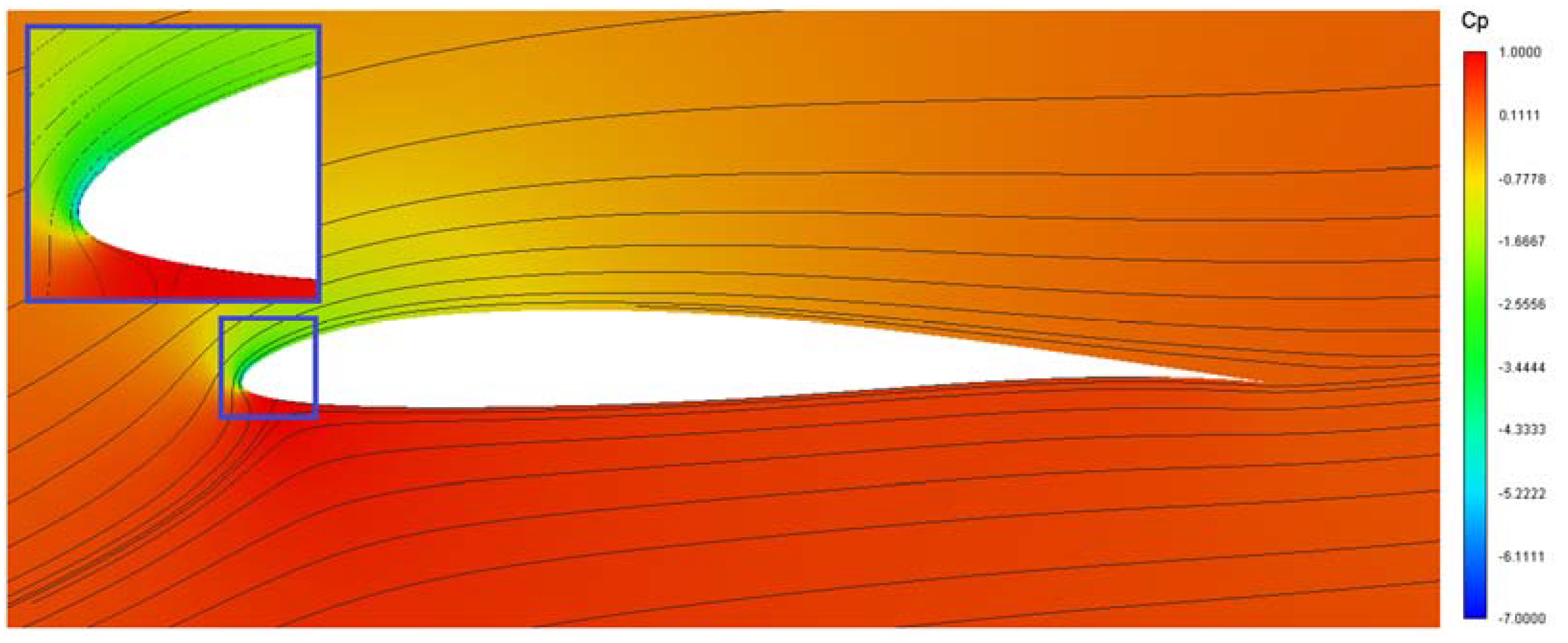
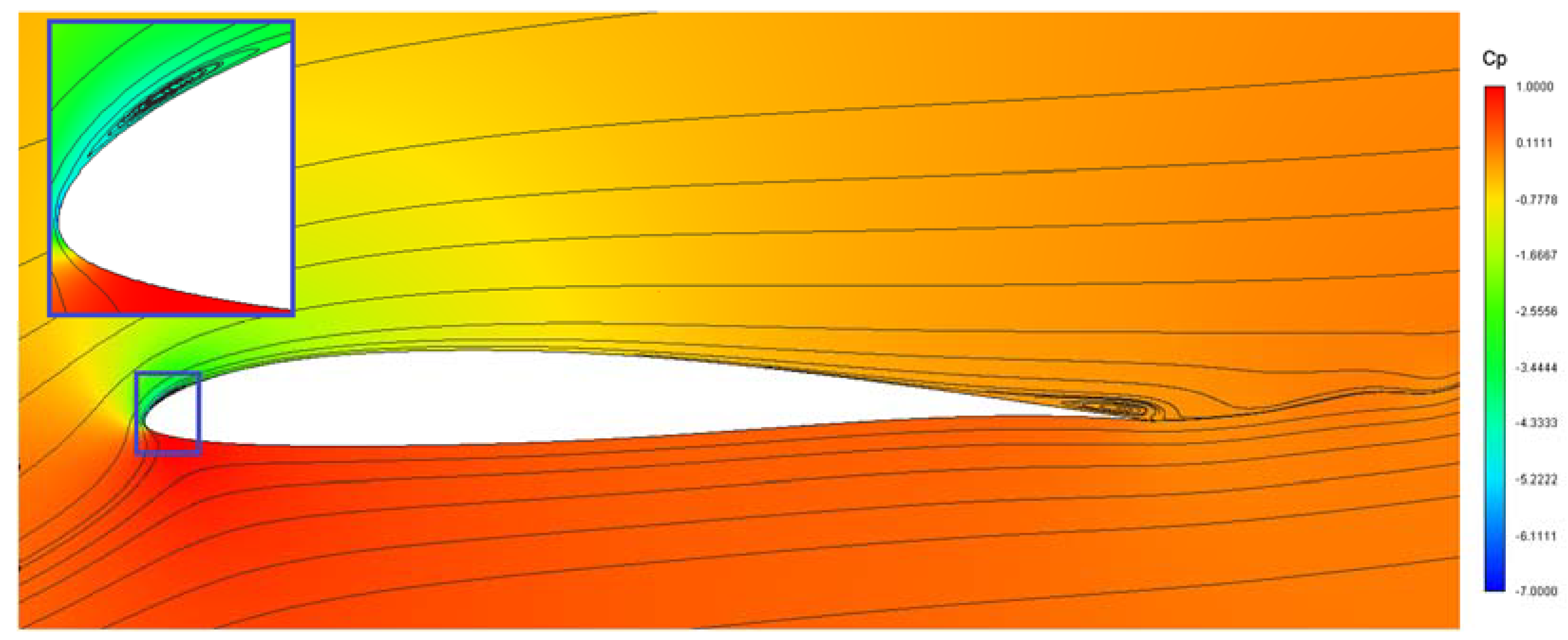
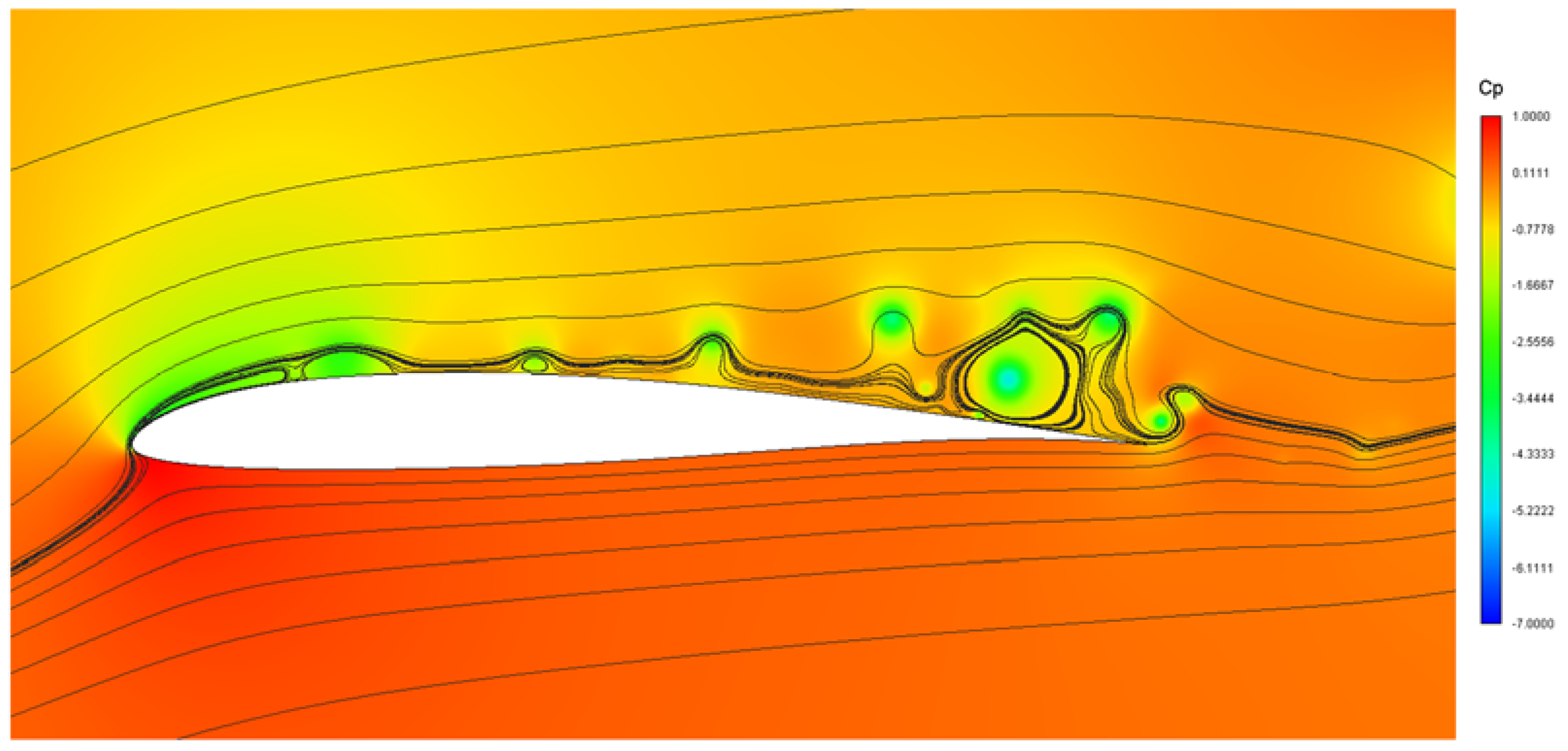
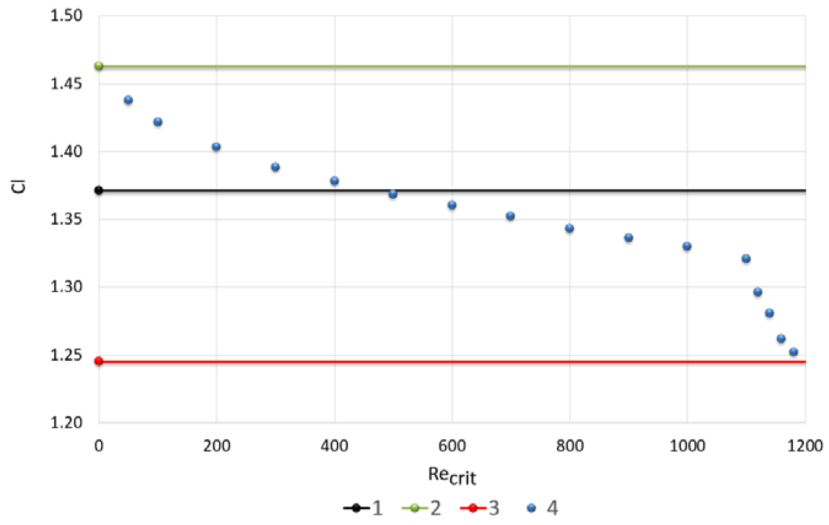
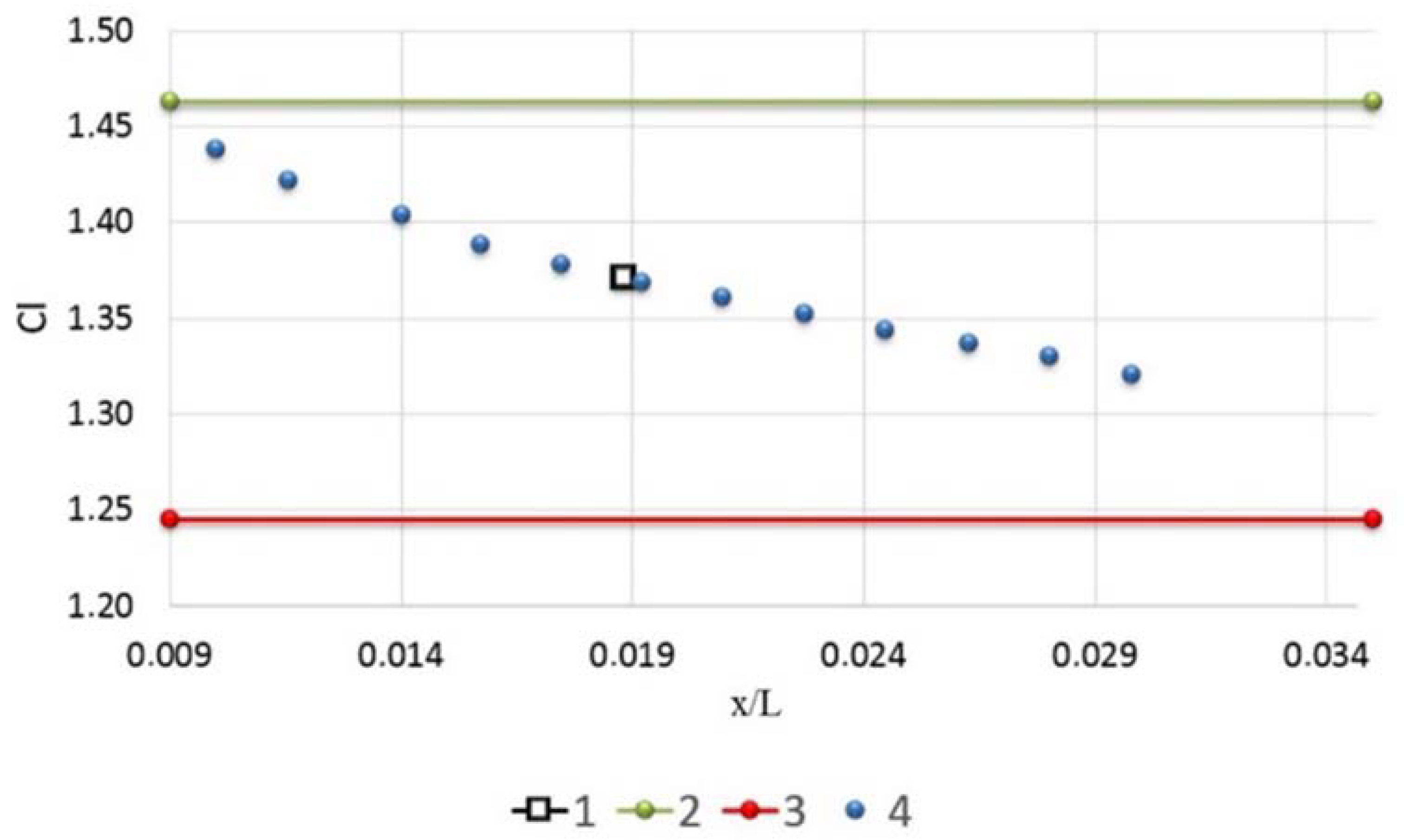
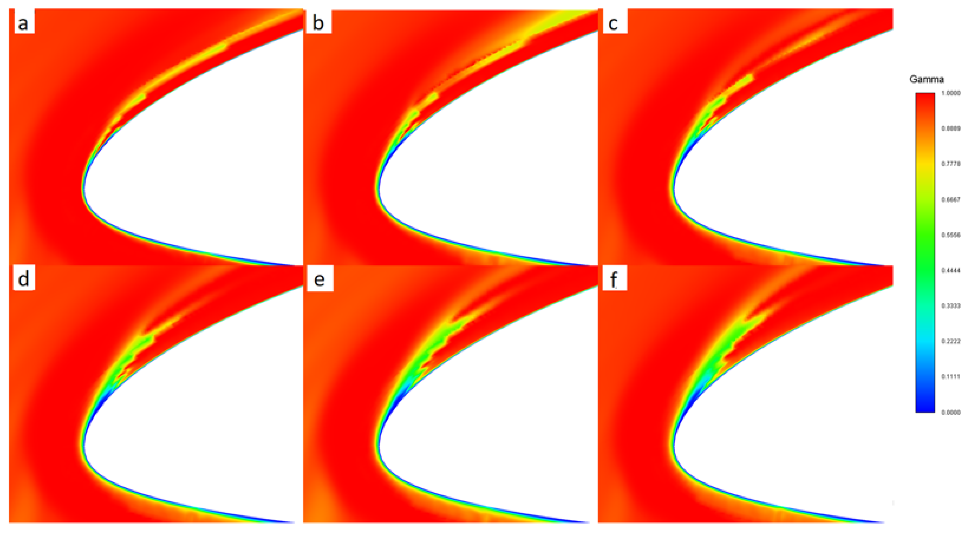
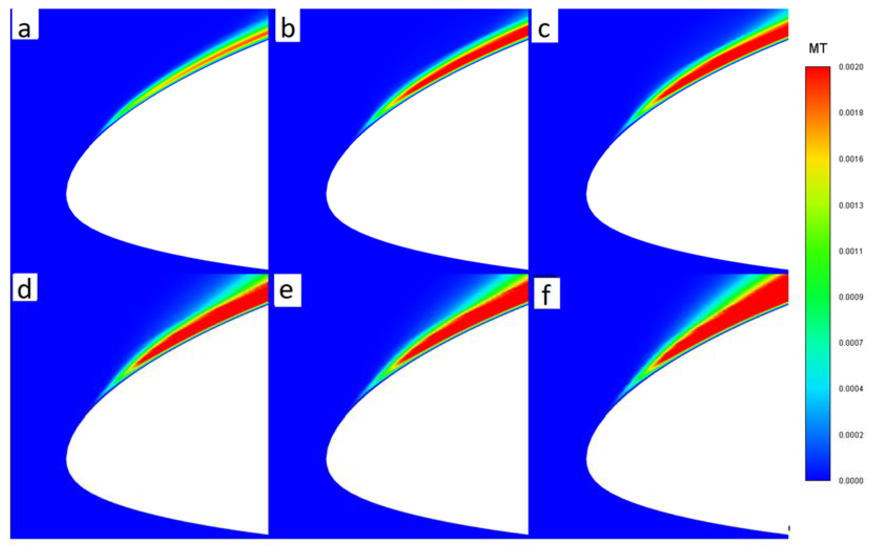
2.2. Numerical Study of the Influence of the Critical Reynolds Number (Recrit) on the Airfoil Aerodynamic Characteristics

The laminar boundary layer can be modeled using the laminar–turbulent transition model γ-Reθt [7,8]. The use of RANS models without the laminar–turbulent transition is impossible in this case, because these models are designed for completely turbulent flows and cannot represent the flow transition from its laminar state to a turbulent one.
In this work, the Recrit parameter is varied in order to control the size of the laminar region. This effect could be achieved by changing the turbulence parameters of the oncoming flow, but, in this case, it is necessary to take into account the effect of turbulence damping when the flow moves from the boundary to the profile. In this investigation, the γ-Reθt model was used in combination with the SSG/LRR-ω RSM turbulence model [12].
Below we will try to trace the influence of the laminar boundary layer on the airfoil aerodynamic characteristics. The numerical experiment makes it possible to investigate the variation of aerodynamic characteristics, such as lift and pressure distribution, with the size of the laminar bubble. A series of calculations were carried out using the turbulence model SSG/LRR-ω at the angle of attack α = 12°, in which the length of the laminar boundary layer varied. Table 1 shows the corresponding design cases.
Figure 6 and Figure 7 show the pressure coefficient distribution and the streamlines for the airfoil at Recrit = 1100 and Recrit = 1120, respectively. Figure 6 shows the characteristic fully attached flow structure at Recrit = 1100. At the leading edge, there is a flow circulation zone in the form of a laminar bubble, which leads to the flow separation and the laminar–turbulent transition. Downstream of the circulation zone, the flow is reattached. With an increase in the critical Reynolds number, the flow does not reattach. Figure 7 shows the structure of the flow at Recrit > 1100, at which there is a separation of the laminar bubble without subsequent attachment.
Figure 8 shows the dependence of the lift coefficient on the critical Reynolds number. The upper vertical line shows the values of the maximum and minimum lift coefficient corresponding to the turbulent and laminar regimes. The middle line shows the value of the lift coefficient corresponding to the given flow parameters in the experiment. It can be seen from the graph that with an increase in the Reynolds number, the value of the lift coefficient tends from a completely turbulent regime to a laminar one, and at Recrit > 1100 there is a sharp decrease in the lift coefficient. This sharp drop in the lift coefficient is due to the fact that the laminar bubble is detached.
Figure 9 shows the dependence of the lift coefficient on the position of the center of the laminar bubble. The position of the bubble center is closest to the experiment in cases No. 5–7.
For a more detailed analysis of the flow behavior, Figure 10 and Figure 11 present the laminar portion of the boundary layer and the turbulent viscosity near the leading-edge. Figure 10 shows that a bubble forms at the leading edge and expands with an increase in the critical Reynolds number. Figure 11 shows that the laminar flow delays the formation of a turbulent boundary layer, which leads to a decrease in the lift coefficient. With an increase in the size of the laminar bubble, the lift coefficient tends from a completely turbulent regime to a laminar one.
The pressure coefficient distribution at the angle of attack α = 12° is shown in Figure 12 for all design cases. The laminar flow also leads to a decrease in the pressure coefficient at the leading edge of the wing. The enlarged part of the pressure coefficient distribution graph in the trailing edge area is shown in the lower right corner of Figure 12b. For most modes, there is a slight deviation of the pressure coefficient on the upper surface of the airfoil, which explains the observed overestimation or underestimation of the lift coefficient from experimental data. In case No. 6, the distribution of the pressure coefficient at the leading edge is closest to the experimental data.
This is most pronounced at the leading and trailing edges of the wing. Figure 13 and Figure 14 show the pressure coefficient distribution at the angle of attack α = 12° for case No. 6, in comparison with the results obtained without taking into account the laminar–turbulent transition model and experimental data.
In the region of the nose and trailing edge of the profile in the turbulent regime, there was the maximum difference from the experimental data, while the laminar–turbulent transition mode (case 6) using the model γ-Reθt made it possible to approach the experimental values.
The numerical analysis provided an insight into the flow structure observed in the experiment. At the leading edge, there is a flow circulation zone in the form of a laminar bubble, which leads to the separation and the laminar–turbulent transition.
The influence of the size of the leading-edge bubble on the aerodynamic characteristics of the airfoil was studied. At Recrit = 1100, the formation of a laminar bubble was observed, which led to the separation and the laminar–turbulent transition. Downstream of the circulation zone, the flow was reattached. With an increase in the size of the laminar bubble, the lift coefficient tended from a completely turbulent regime to a laminar one. At Recrit > 1100, there was a separation of the laminar bubble without subsequent attachment.
The numerical results obtained at Recrit = 500 are in good agreement with the experimental data. For Recrit = 500, the length of the laminar portion of the boundary layer is 0.0192 m.

3. Conclusions

A study is made of the features of the flow around the HGR01 airfoil using various turbulence models. It is shown that in the presence of complex flow regimes, the Spalart–Allmaras model based on the Boussinesq hypothesis gives a result that is far from the experimental data. More complex nonlinear turbulence models also do not allow one to achieve a qualitative description of the flow structure near the airfoil, although the trend towards a decrease in lift can already be traced.
A significant problem in the numerical experiment is the description of the laminar bubble near the leading edge. None of the RANS models show the presence of the laminar separation bubble in this area.
The correct behavior of the flow in the calculation is obtained only using the laminar–turbulent transition model. It has been established that the size of the separation region in the region of the leading edge depends significantly on the critical Reynolds number.
The results of a study of the dependence of the influence of the bubble size near the nose of the HGR01 airfoil on its aerodynamic characteristics are presented. The structure of the flow is shown as a function of the critical Reynolds number along the profile. The dependence of the lifting force on the size of the bubble is obtained. Graphs of the dependence of the lift force coefficient on the critical Reynolds number are presented, as well as the pressure distribution on the profile on the size of the laminar bubble on the profile. The paper demonstrates that a decreasing critical Reynolds number leads to a larger laminar section in the front part of the airfoil that, in turn, leads to a lower value of the lift coefficient. With an increased size of this section, the lift coefficient tends to change its value from that for the completely turbulent to the laminar flow conditions.

Author Contributions

Conceptualization, A.U. and A.K.; methodology, A.U. and R.Z.; software, A.K.; validation, R.Z. and D.S.; formal analysis, A.K. and D.S.; investigation, A.U.; resources, R.Z.; data curation, A.K.; writing—original draft preparation, A.U.; writing—review and editing, A.U., A.K. and D.S.; visualization, R.Z. All authors have read and agreed to the published version of the manuscript.

Funding

The work is prepared in the implementation of the program for the creation and development of the World-Class Research Center “Supersonic” for 2020–2025 funded by the Ministry of Science and Higher Education of the Russian Federation (Grant agreement of 20 April 2022 № 075-15-2022-309). The results have been obtained with financial support from the Science and Universities National Project under the Young Scientists Lab Program of the RF Ministry of Education and Science—project identifier № FSWE-2021-0009 (Research topic: development of CFD methods, models and algorithms to simulate liquids and gases in natural and industrial environments under normal and critical conditions on petascale supercomputers) and the Council of the Grants of the President of the Russian Federation for state support of Leading Scientific Schools of the Russian Federation (Grant № NSH-70.2022.1.5).

Data Availability Statement

Not acceptable.

Conflicts of Interest

The authors declare no conflict of interest.

References

  1. Wokoeck, R.; Krimmelbein, N.; Radespiel, R.; Ciobaca, V.; Krumbein, A. RANS Simulation and Experiments on the Stall Behaviour of an Airfoil with Laminar Separation Bubbles. In Proceedings of the 44th AIAA Aerospace Sciences Meeting and Exhibit, Reno, NV, USA, 9–12 January 2006. [Google Scholar]
  2. Baragona, M.; Boermanns, L.M.M.; van Tooren, M.J.L.; Bijl, H.; Beukers, A. Bubble Bursting and Stall Hysteresis on Single-Slotted Flap High Lift Configuration. AIAA J. 2003, 41, 1230–1237. [Google Scholar] [CrossRef]
  3. Broeren, A.P.; Bragg, M.B. Spanwise Variation in the Unsteady Stalling Flowfields of Two-Dimensional Airfoil Models. AIAA J. 2001, 39, 1641–1651. [Google Scholar] [CrossRef]
  4. Spalart, P.R. Strategies for turbulence modeling and simulations. Int. J. Heat Fluid Flow 2020, 21, 252–263. [Google Scholar] [CrossRef]
  5. Spalart, P.R.; Allmaras, S.R. A one-equation turbulence model for aerodynamic flows. In Proceedings of the 30th Aerospace Sciences Meeting and Exhibit, Reno, NV, USA, 6–9 January 1992. [Google Scholar]
  6. Menter, F.R. Zonal two equation k-w turbulence models for aerodynamic flows. In Proceedings of the 23rd Fluid Dynamics, Plasmadynamics, and Lasers Conference, Orlando, FL, USA, 6–9 July 1993. [Google Scholar]
  7. Langtry, R.B.; Menter, F.R. Transition Modeling for General CFD Applications in Aeronautics. In Proceedings of the 43rd AIAA Aerospace Sciences Meeting and Exhibit, Reno, NV, USA, 10–13 January 2005. [Google Scholar]
  8. Langtry, R.B.; Menter, F.R. Correlation-Based Transition Modeling for Unstructured Parallelized Computational Fluid Dynamics Codes. AIAA J. 2009, 47, 2894–2906. [Google Scholar] [CrossRef]
  9. Menter, F.R.; Langtry, R.B.; Likki, S.R.; Suzen, Y.B.; Huang, P.G.; Völker, S. A Correlation based Transition Model using Local Variables. Part 1: Model Formulation. J. Turbomach. 2006, 128, 413–422. [Google Scholar] [CrossRef]
  10. Langtry, R.B. A Correlation-Based Transition Model Using Local Variables for Unstructured Parallelized CFD Codes. Ph.D. Thesis, Institute of Thermal Turbomachinery and Machinery Laboratory, University of Stuttgart, Stuttgart, Germany, 2006. Available online: https://elib.unistuttgart.de/opus/volltexte/2006/2801/ (accessed on 1 January 2020).
  11. Cecora, R.-D.; Eisfeld, B.; Probst, A.; Crippa, S.; Radespiel, R. Differential Reynolds Stress. In Proceedings of the 50th AIAA Aerospace Sciences Meeting including the New Horizons Forum and Aerospace Exposition, Nashville, TN, USA, 9–12 January 2012. [Google Scholar]
  12. Zhuchkov, R.N.; Utkina, A.A. Combining the differential SSG/LRR-ω Reynolds stress model with models of detached vortices and laminar-turbulent transition. J. Fluid Gas Mech. 2016, 51, 25–35. [Google Scholar]
  13. Utkina, A.A.; Zhuchkov, R.N.; Deryugin, Y.N.; Emelyanova, Y.V. Application of hybrid dissipation scheme in solving computational aeroacoustics problems. J. Comput. Math. Math. Phys. 2018, 58, 1478–1487. [Google Scholar]
  14. Struchkov, A.V.; Kozelkov, A.S.; Volkov, K.; Kurkin, A.A.; Zhuchkov, R.N.; Sarazov, A.V. Numerical simulation of aerodynamic problems based on adaptive mesh refinement method. Acta Astronaut. 2020, 172, 7–15. [Google Scholar] [CrossRef]
  15. Kozelkov, A.S.; Pogosyan, M.A.; Strelets, D.Y.; Tarasova, N.V. Application of mathematical modeling to solve the emergency water landing task in the interests of passenger aircraft certification. Aerosp. Syst. 2021, 4, 75–89. [Google Scholar] [CrossRef]
  16. Tyatyushkina, E.S.; Kozelkov, A.S.; Kurkin, A.A.; Pelinovsky, E.N.; Kurulin, V.V.; Plygunova, K.S.; Utkin, D.A. Verification of the LOGOS Software Package for Tsunami Simulations. Geosciences 2020, 10, 385. [Google Scholar] [CrossRef]
  17. Kozelkov, A.S.; Strelets, D.Y.; Sokuler, M.S.; Arifullin, R.H. Application of Mathematical Modeling to Study Near-Field Pressure Pulsations of a Near-Future Prototype Supersonic Business Aircraft. J. Aerosp. Eng. 2022, 35, 04021120. [Google Scholar] [CrossRef]
  18. Probst, A.; Radespiel, R.; Wolf, C.; Knopp, T.; Schwamborn, D. A Comparison of Detached-Eddy Simulation and Reynolds-Stress Modelling Applied to the Flow over a Backward-Facing Step and an Airfoil at Stall. In Proceedings of the 48th AIAA Aerospace Sciences Meeting Including the New Horizons Forum and Aerospace Exposition, Orlando, FL, USA, 4–7 January 2010. [Google Scholar]
Figure 1. Computational domain.
Fluids 08 00276 g001
Figure 2. Lift curve: 1—experimental data [11], 2—SA, 3—SSG/LRR-ω, 4—SSG/LRR-ω [11], 5—JHh-v2 [11].
Fluids 08 00276 g002
Figure 3. Streamlines near the trailing edge of the HGR01 airfoil: (a)—PIV measurements [1], (b)—SA, (c)—SSG/LRR-ω.
Fluids 08 00276 g003
Figure 4. Leading-edge flow visualization in the experiment.
Fluids 08 00276 g004
Figure 5. Pressure coefficient distribution and streamlines for the HGR01 airfoil at an angle of attack of 12°.
Fluids 08 00276 g005
Figure 6. Pressure coefficient distribution and streamlines for the HGR01 airfoil at Recrit = 1100.
Fluids 08 00276 g006
Figure 7. Pressure coefficient distribution and streamlines for the HGR01 airfoil at Recrit = 1120.
Fluids 08 00276 g007
Figure 8. Lift coefficient versus the critical Reynolds number: 1—experimental data [11], 2—turbulent mode (SSG/LRR-ω), 3—laminar mode, 4—SSG/LRR-ω at different Recrit.
Fluids 08 00276 g008
Figure 9. Lift coefficient versus the position of the center of the laminar separation bubble: 1—experimental data [11], 2—turbulent mode (SSG/LRR-ω), 3—laminar mode, 4—SSG/LRR-ω at different Recrit.
Fluids 08 00276 g009
Figure 10. Laminar boundary layer: (a)—No. 2, (b)—No. 4, (c)—No. 6, (d)—No. 8, (e)—No. 10, (f)—No. 12.
Fluids 08 00276 g010
Figure 11. Distribution of turbulent viscosity: (a)—No. 2, (b)—No. 4, (c)—No. 6, (d)—No. 8, (e)—No. 10, (f)—No. 12, P a · s .
Fluids 08 00276 g011
Figure 12. Pressure coefficient distribution for the airfoil (a) and the enlarged part of the graph in the leading-edge area (b) at the angle of attack α = 12°: 1—experimental data [18], 2–13—No. 1–12.
Fluids 08 00276 g012
Figure 13. Leading-edge pressure distribution at the angle of attack α = 12°: 1—experimental data [14], 2—turbulent mode, 3—laminar–turbulent mode (No. 6).
Fluids 08 00276 g013
Figure 14. Trailing-edge pressure distribution at the angle of attack α = 12°: 1—experimental data [14], 2—turbulent mode, 3—laminar–turbulent mode (No. 6).
Fluids 08 00276 g014
Table 1. Design cases.
No.RecritNo.RecritNo.RecritNo.Recrit
15054009800131120
2100650010900141140
32007600111000151160
43008700121100161180
Disclaimer/Publisher’s Note: The statements, opinions and data contained in all publications are solely those of the individual author(s) and contributor(s) and not of MDPI and/or the editor(s). MDPI and/or the editor(s) disclaim responsibility for any injury to people or property resulting from any ideas, methods, instructions or products referred to in the content.

