
Parametrization Effects of the Non-Linear Unsteady Vortex Method with Vortex Particle Method for Small Rotor Aerodynamics

Abstract
:1. Introduction
- 1.
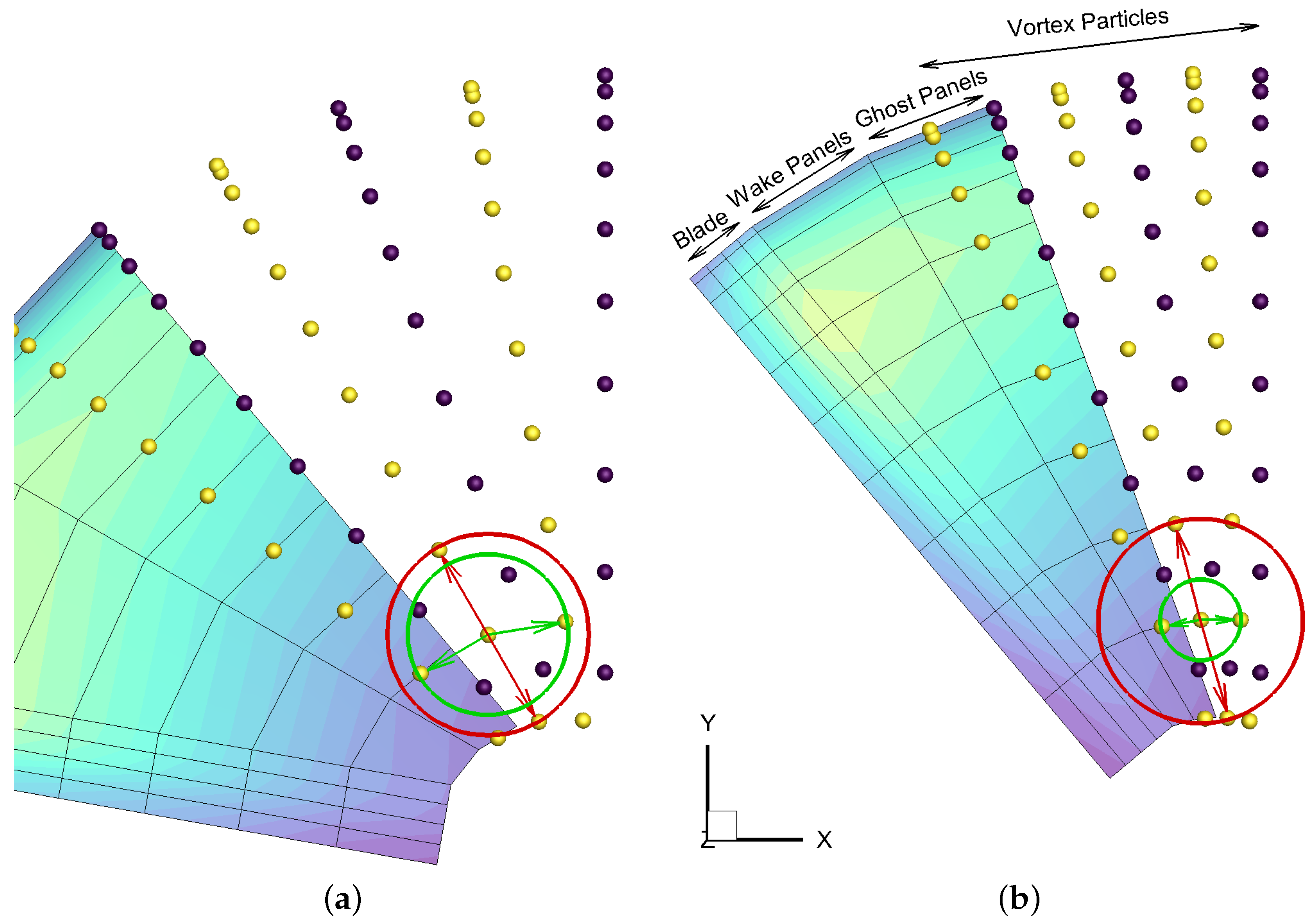
- UVLM Vatistas core size (): It was not needed in the previous work, because the wake panels were instantly converted into particles. In the present work, some rows of wake panels are kept behind the blade to help reduce the near-field discretization error of the velocity induced on the blades because the discrete particles approximation of the straight-line vortex elements are now farther from the rotor plane. Reducing the impact of particles on the blade allows coarser particles discretization than before. However, the prescribed Vatistas core size provided to smooth the wake panels induced velocity singularity needs to be carefully selected to achieve stability without significantly affecting the results;
- 2.
- Geometry discretization refinement (mesh): In the previous work, the geometry discretization refinement was conducted simultaneously with the time discretization refinement. The method appeared to be consistent with refinement. After the publication, it was realized that independently varying the geometry and time discretizations was not consistent. The reasons for this inconsistency and the solution to the problem are detailed at the beginning of Section 3.2;
- 3.
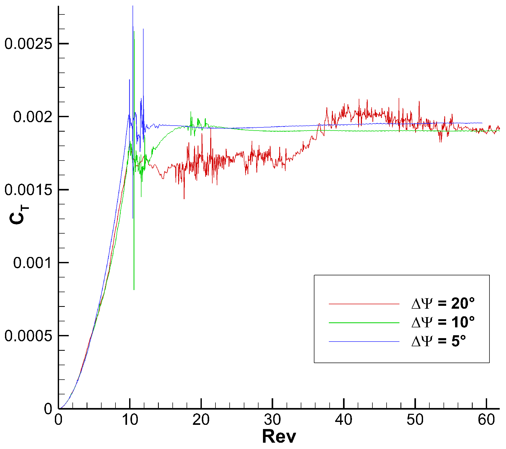
- Time discretization refinement (time step, ):where is the azimuthal increment per time step in degree, is the time step in seconds and is the rotational speed in degree per second. It was previously performed jointly with the geometry discretization refinement;
- 4.
- Vreman model coefficient (): In the previous work, the Vreman model coefficient was set to 0.07 as it is the equivalent value to the theoretical value of the Smagorinsky constant for homogeneous isotropic turbulence. The theoretical value kept all the simulations stable, so it was thought to be appropriate. However, the theoretical value did not keep the VPM stability on the smaller radius and aspect ratio rotor of the current work. Vreman states that to obtain robust simulations for complex practical cases, the value can be higher or lower than the theoretical value [6]. In this work, it is observed that the value needed for this constant varies with the tip particle spacing;
- 5.
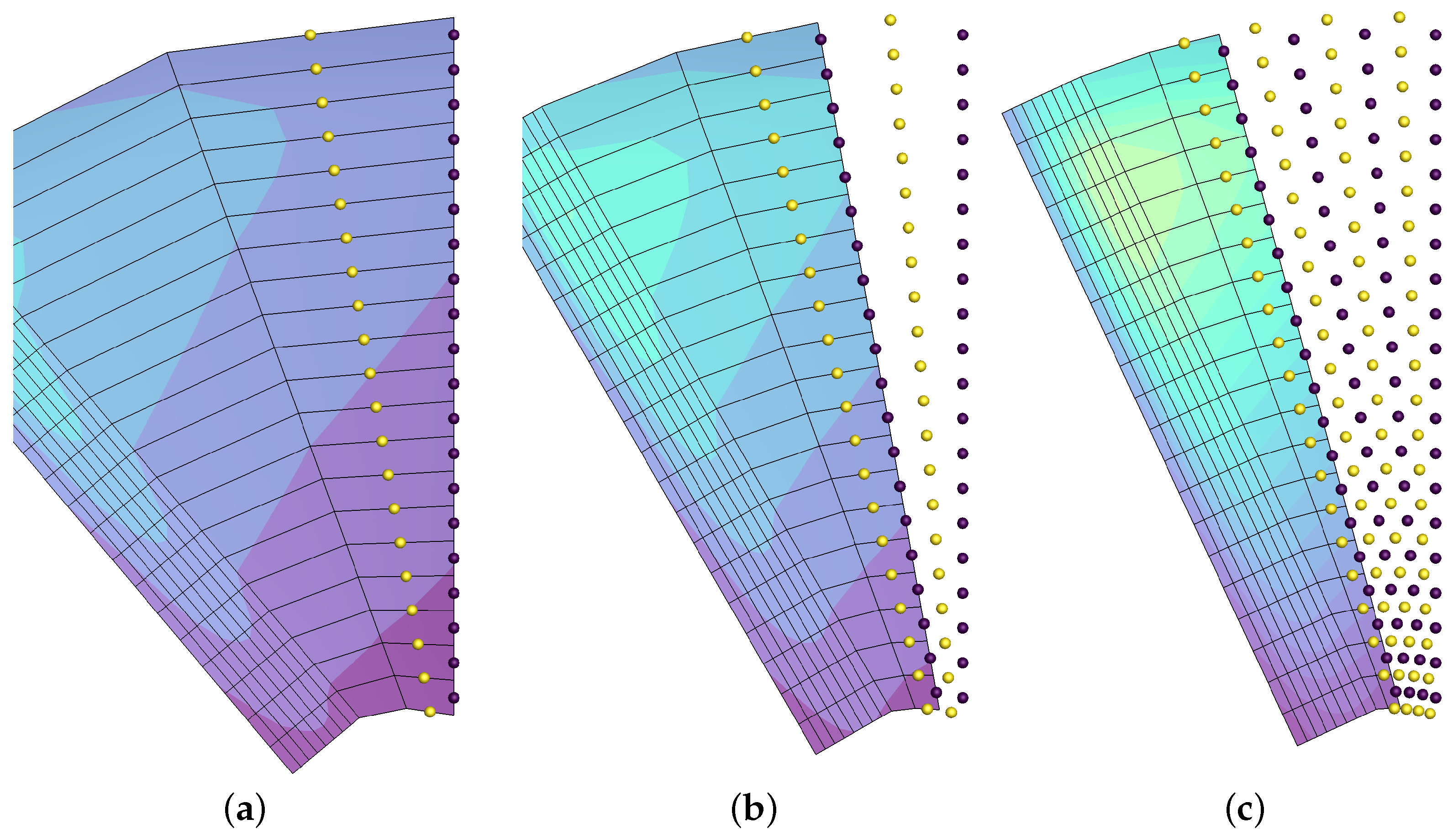
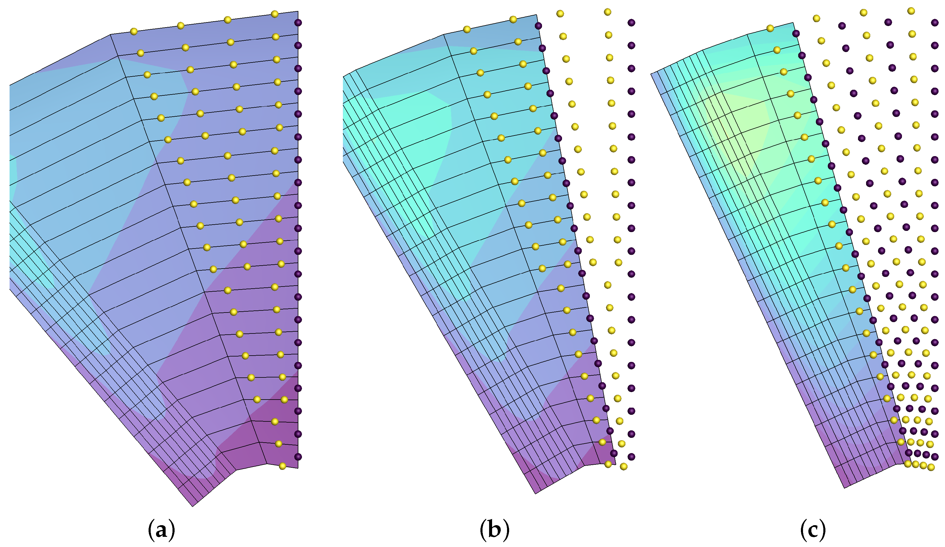
- Tip particle spacing ():where is the tip particle spacing and is the number of streamwise particles per time step at the tip of the blade. In the previous work, a straight-line vortex line was always converted in a single particle, therefore it was not possible to test that parameter independently from the time step. The time step was much smaller, so it was a reasonable simplification. With the larger time step used in this work, it is important to have multiple particles on the longer straight-line elements to avoid discretizing them with a single enormous discrete particle;
- 6.
- Wake-particle conversion time (revolution): In the previous work, the wake panels were instantly converted into particles, so that parameter was not present. In the current work, keeping the wake panels helps to increase the time step by moving farther from the rotor plane the discretization error caused by the discrete particles;
- 7.
- Database for the non-linear coupling: Two different databases were tested along with the linear UVLM in the previous work. In this work, since the parametric study focuses on a single case, four different databases are tested in the Results section of the present article.
2. Literature Comparison
2.1. Similar Methods Summary
2.2. Similar Methods Validation Cases
2.3. Similar Methods Validation Comparison
2.4. Conclusion of the Literature Comparison
3. Method
3.1. Previous Method Summary
3.2. Method Improvements
4. Test Case
4.1. Definition
4.2. Database Generation
5. Parametrization
5.1. Parametrization of the UVLM
5.1.1. UVLM Vatistas Core Size
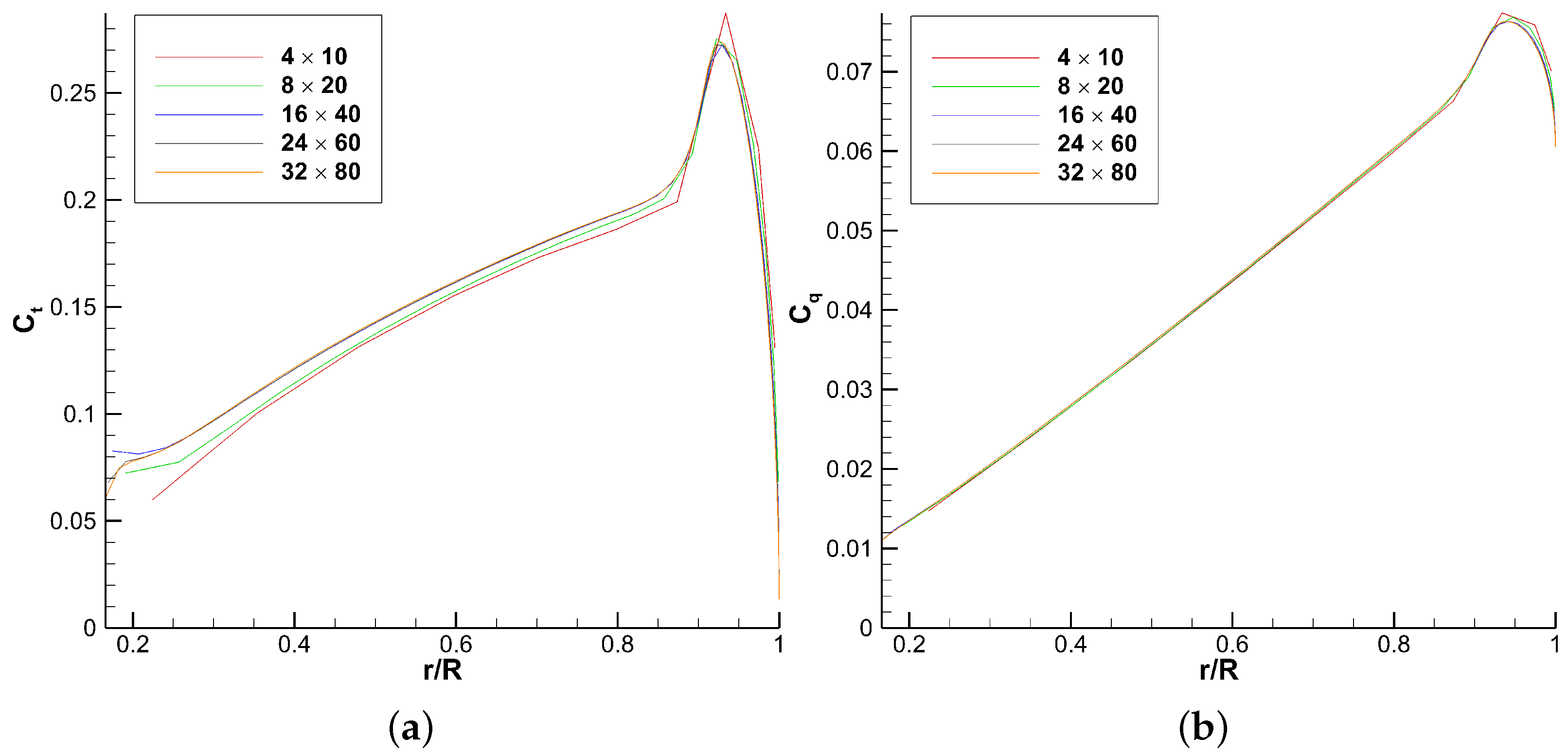
5.1.2. UVLM Mesh Refinement
5.1.3. NL-UVLM Time Refinement
5.1.4. NL-UVLM Vatisas Verification
5.1.5. Summary of the UVLM Parametrization
5.2. Parametrization of the UVLM-VPM
5.2.1. UVLM-VPM Vreman Model Coefficient Stability at Constant
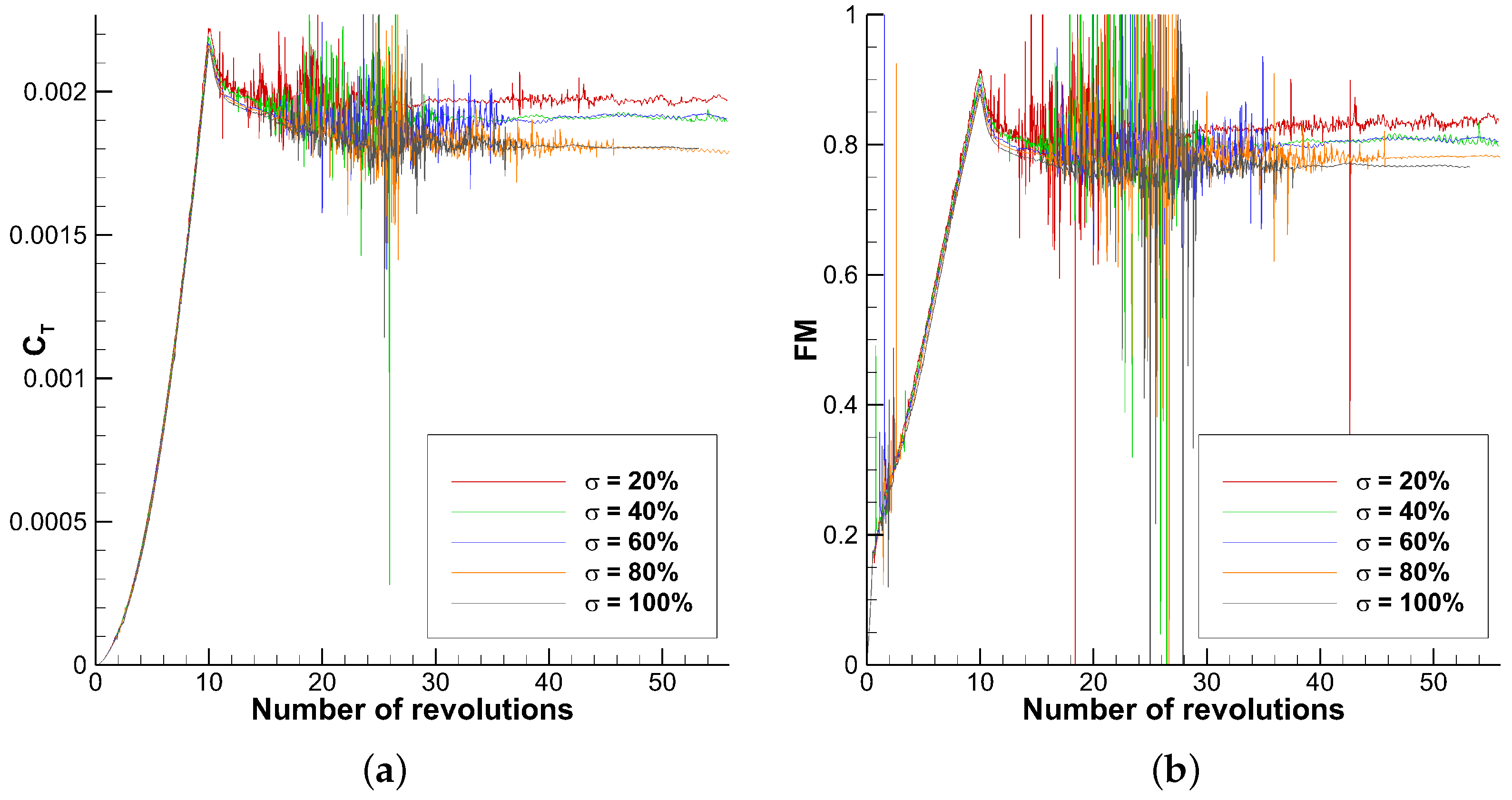
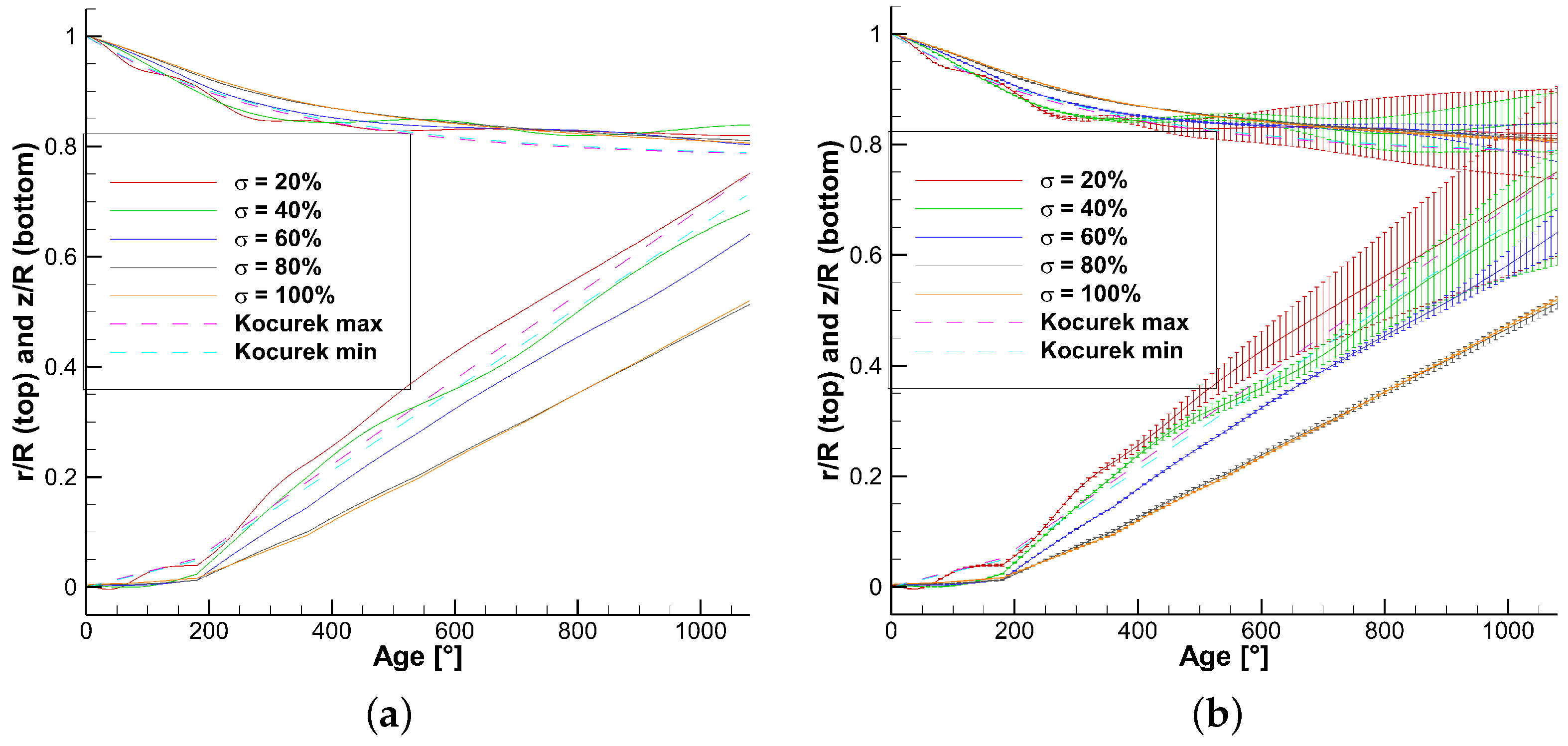
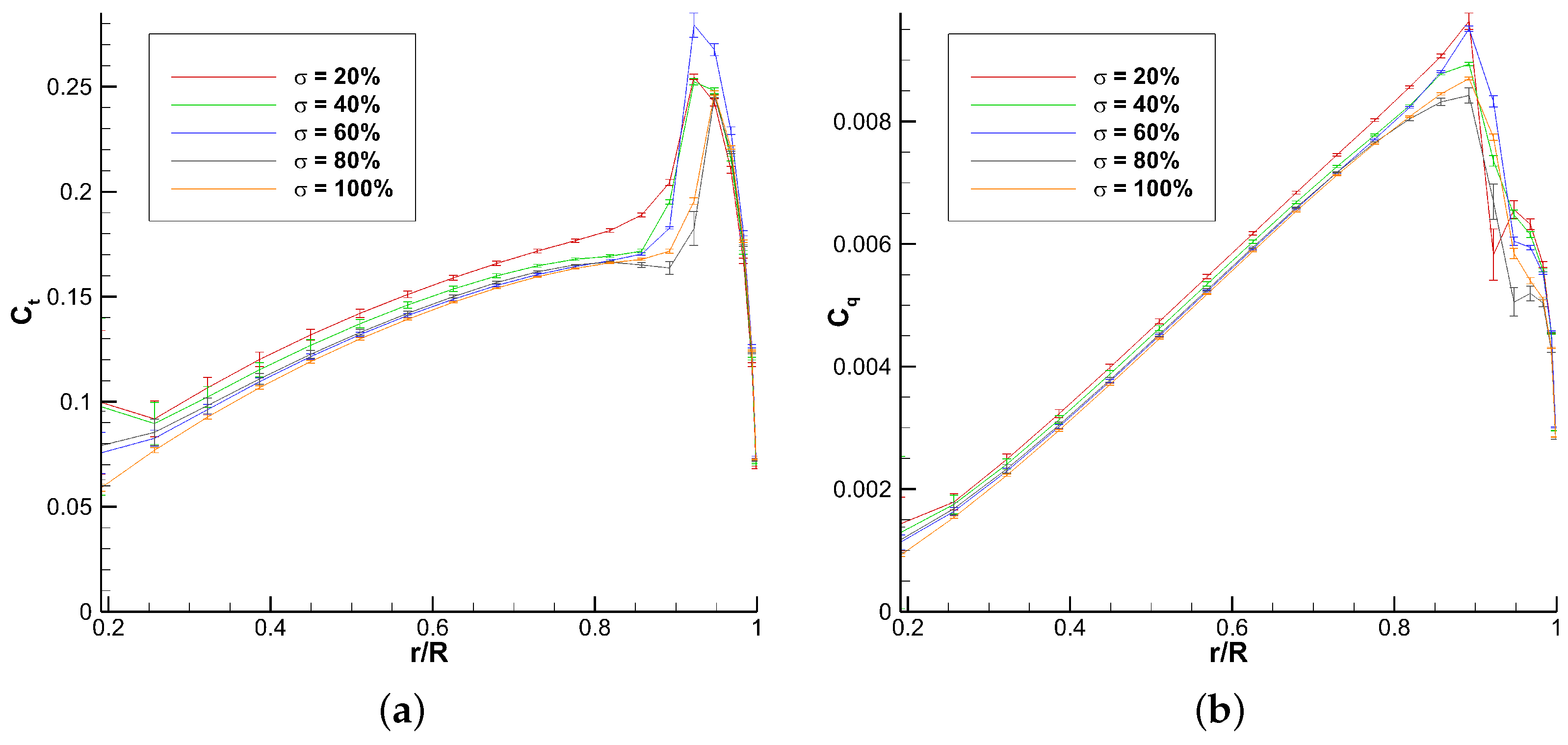
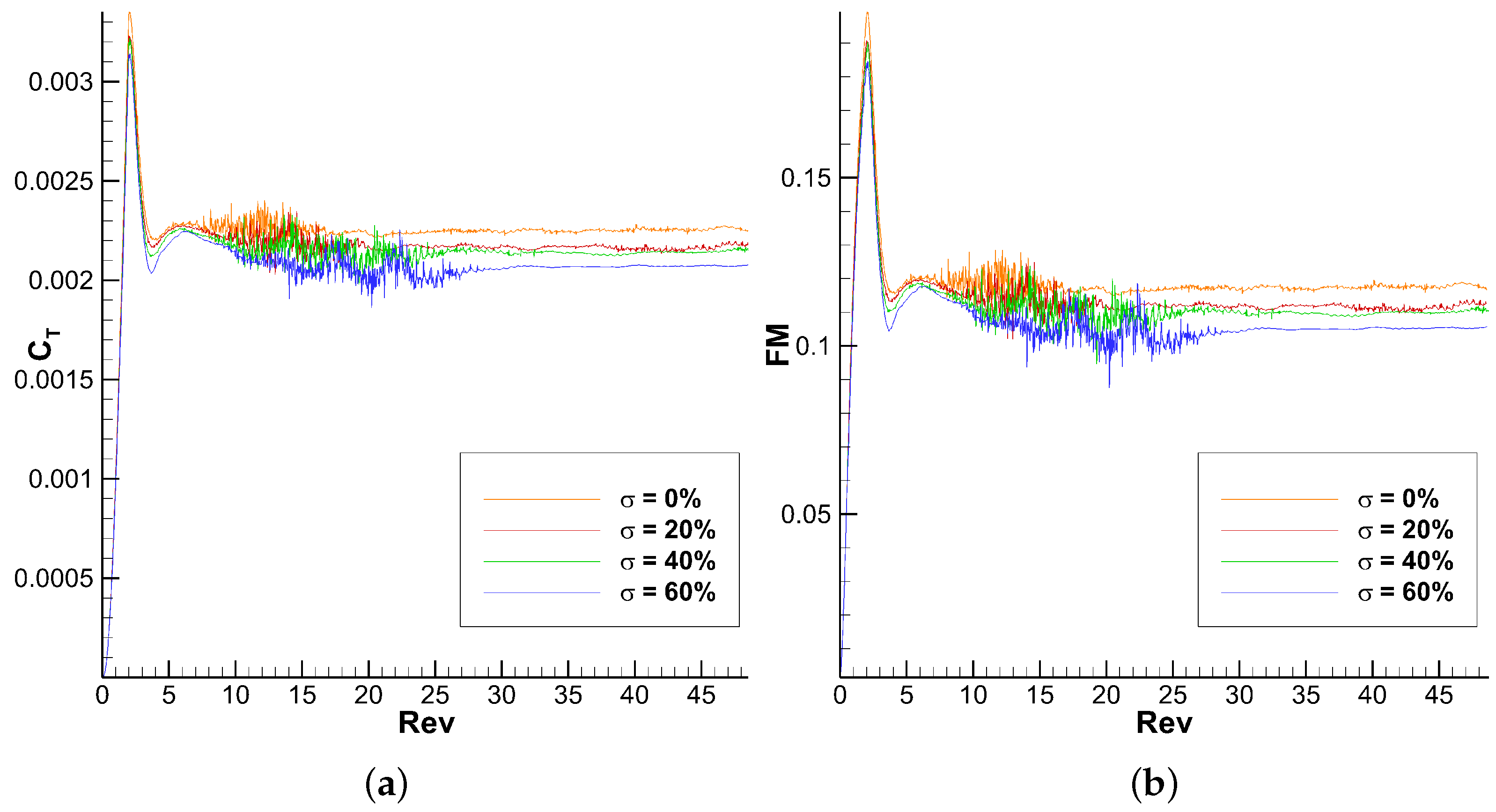
5.2.2. NL-UVLM-VPM Tip Vortex Particle Refinement () at Constant Time Step ()
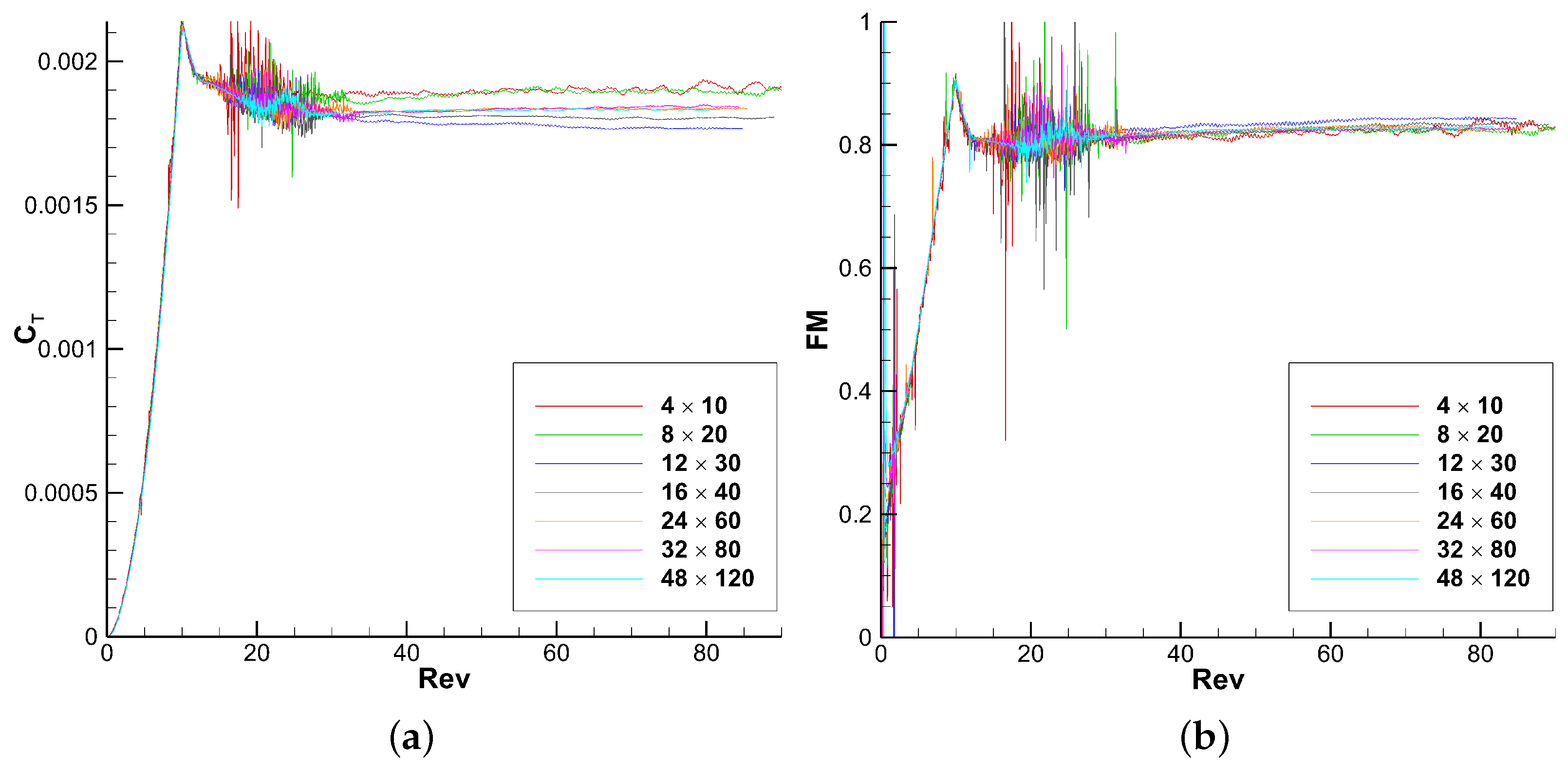
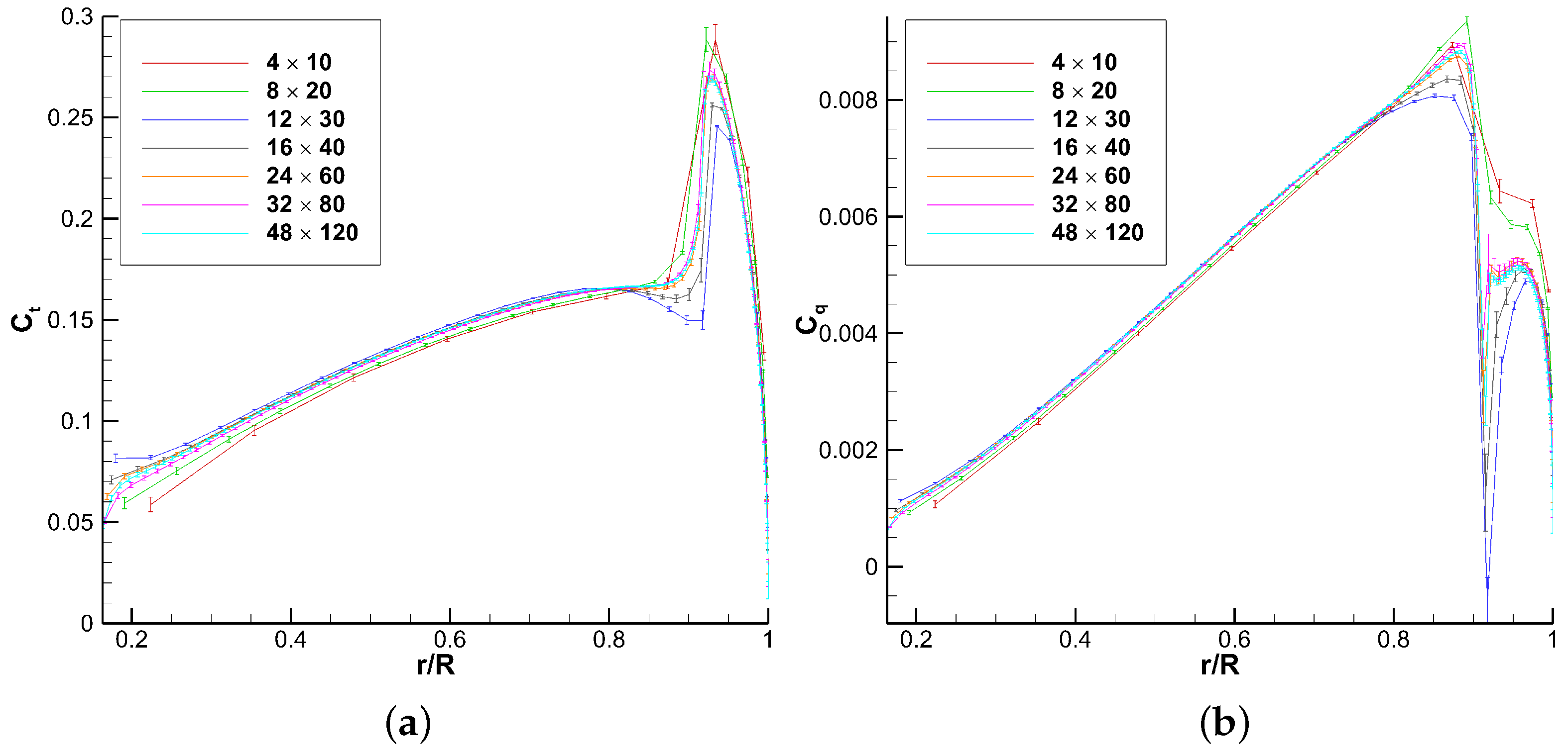
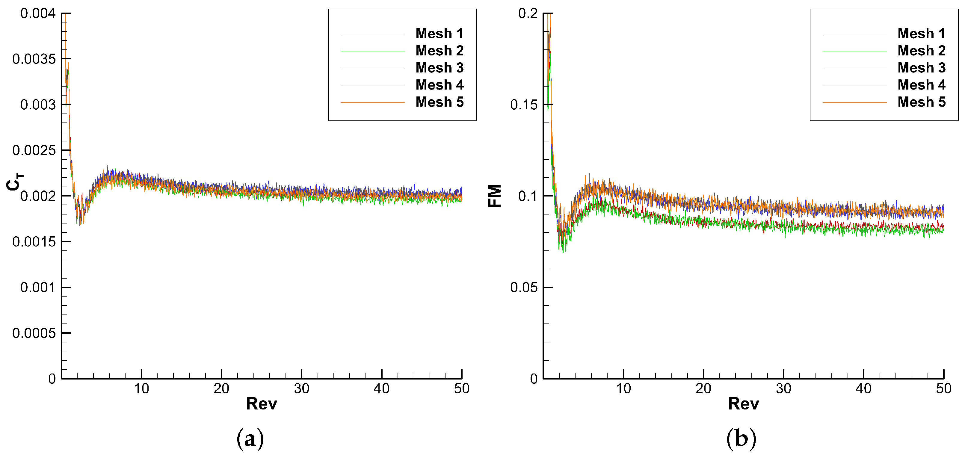
5.2.3. NL-UVLM-VPM Mesh Convergence
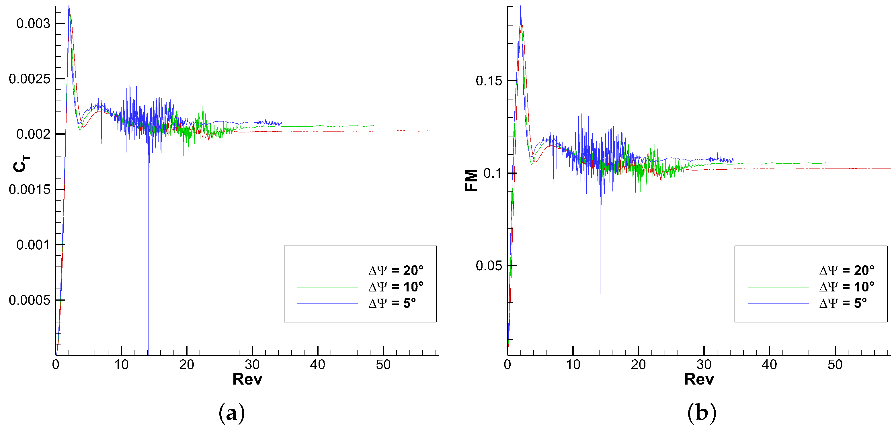
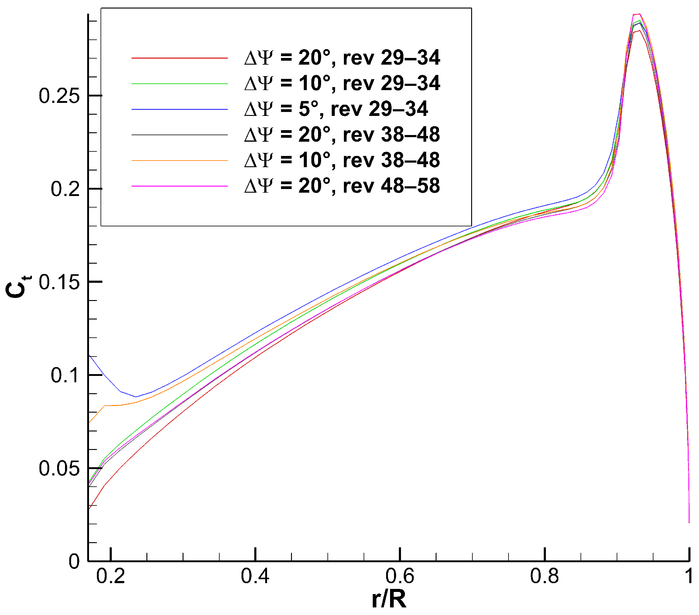
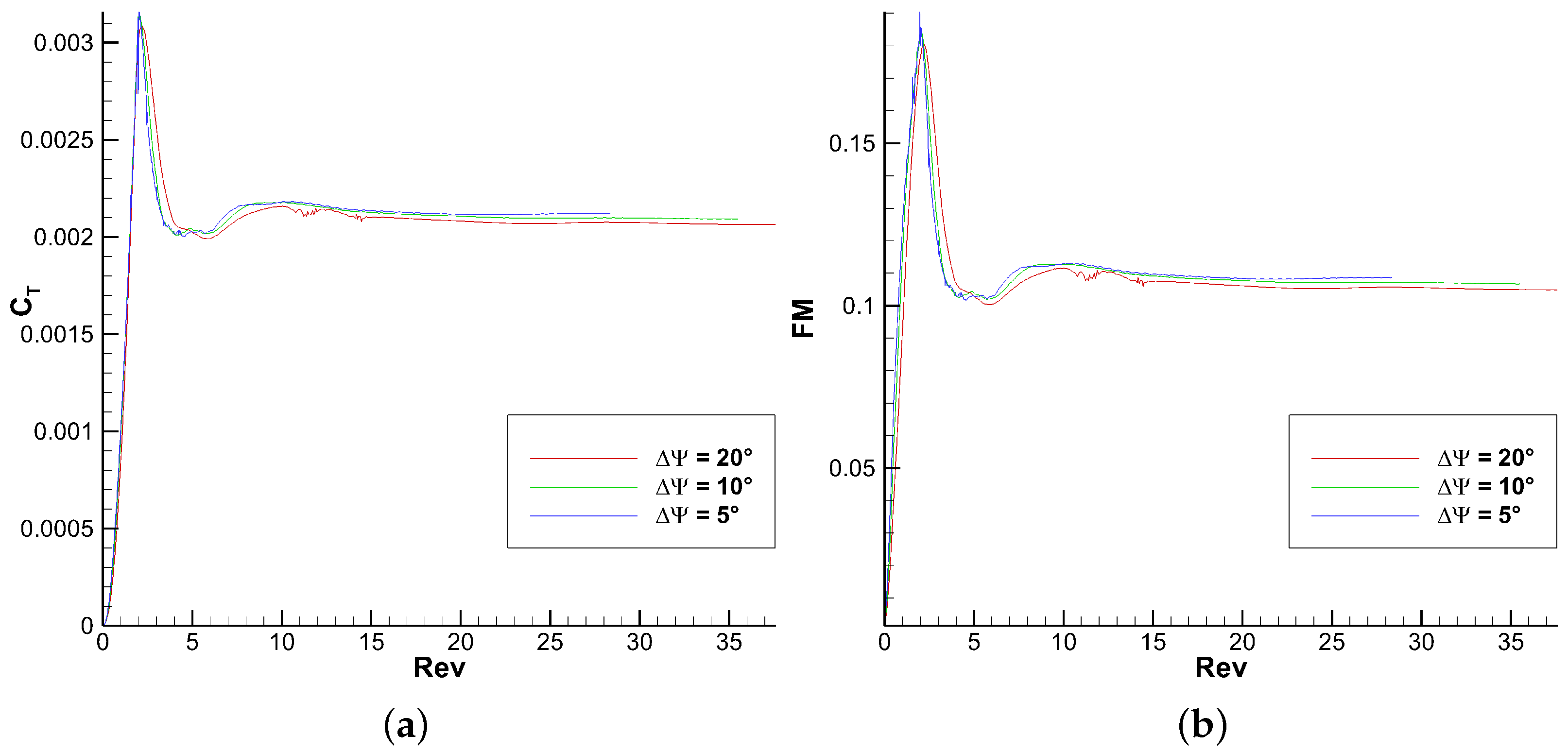
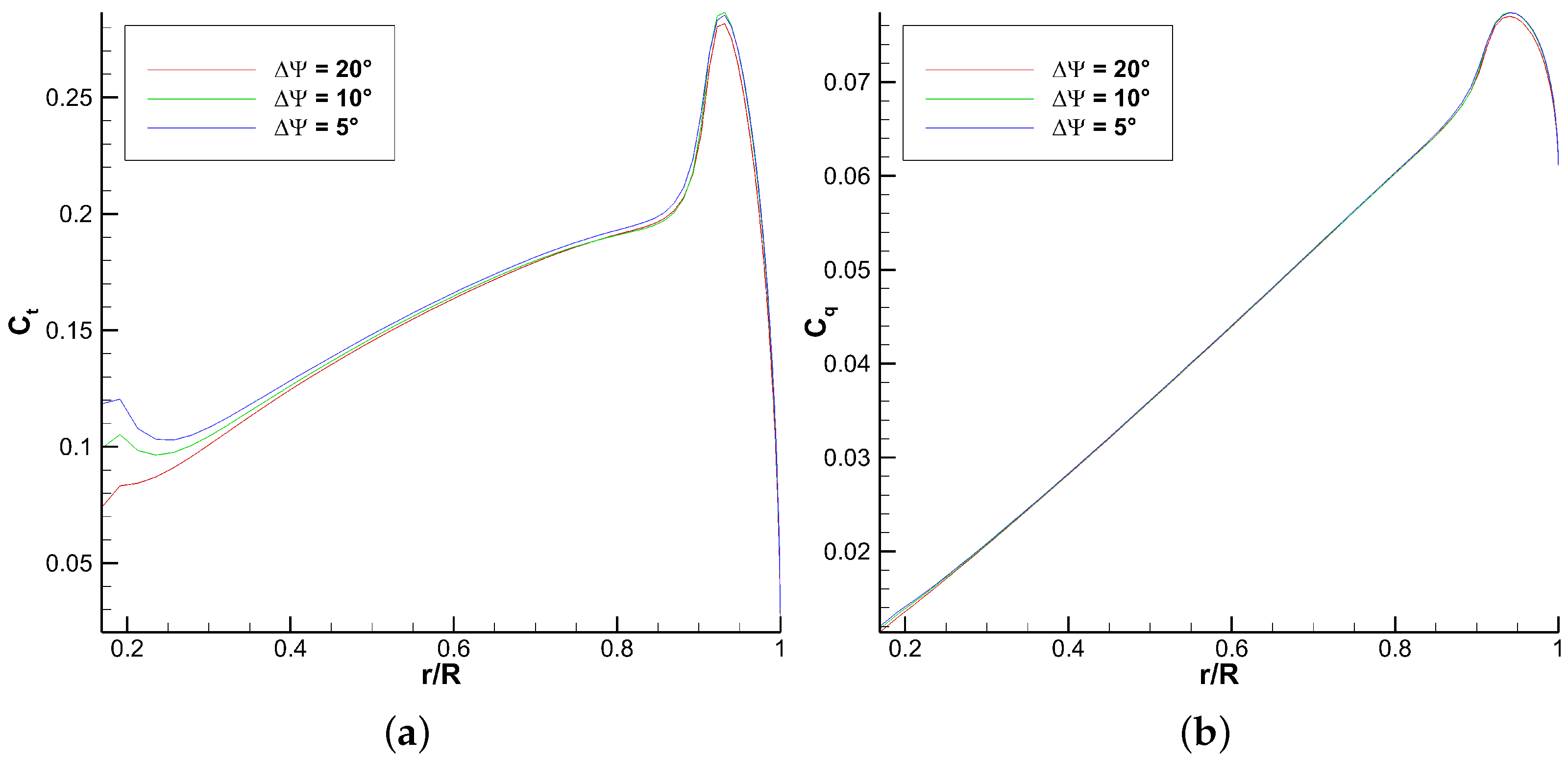
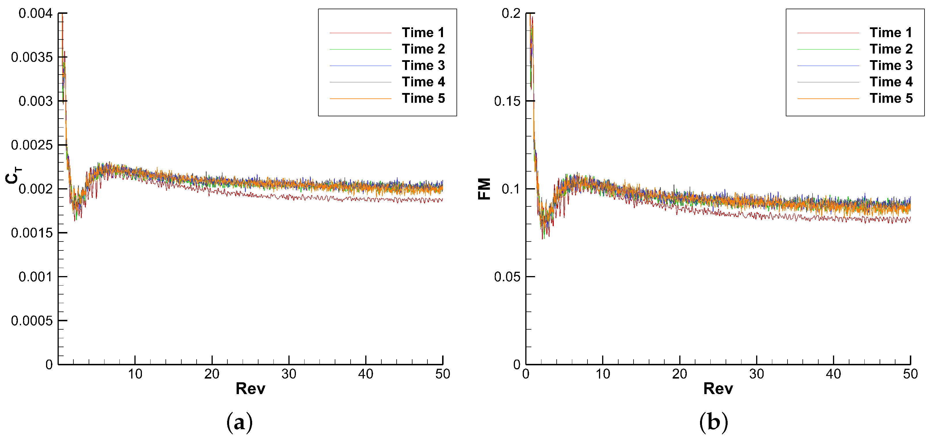
5.2.4. NL-UVLM-VPM Time Convergence
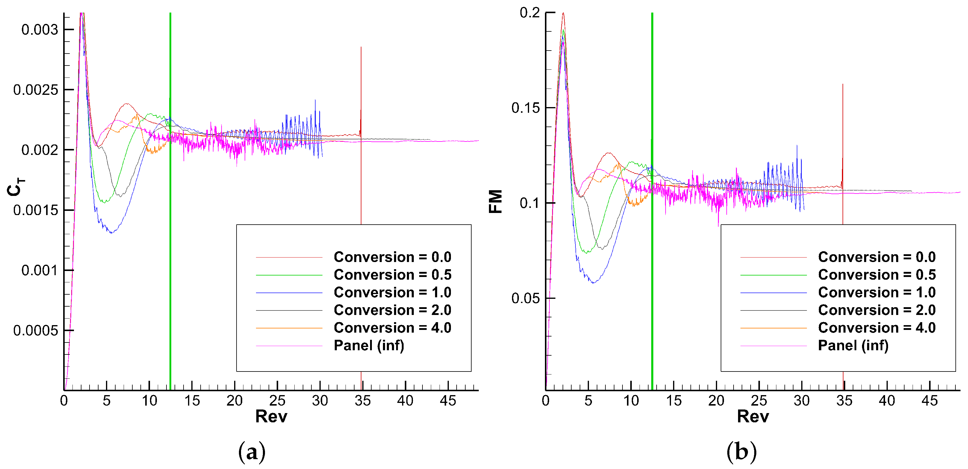
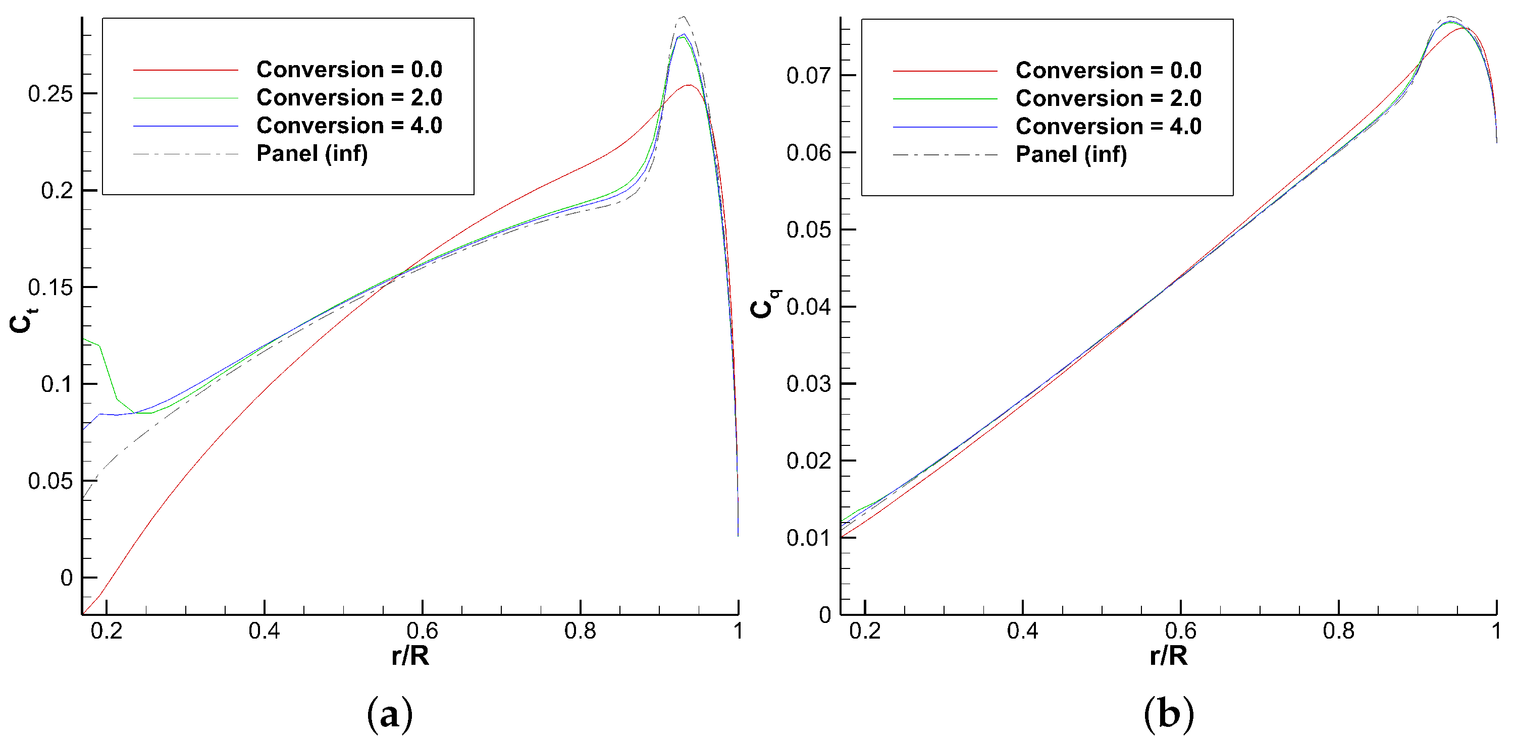
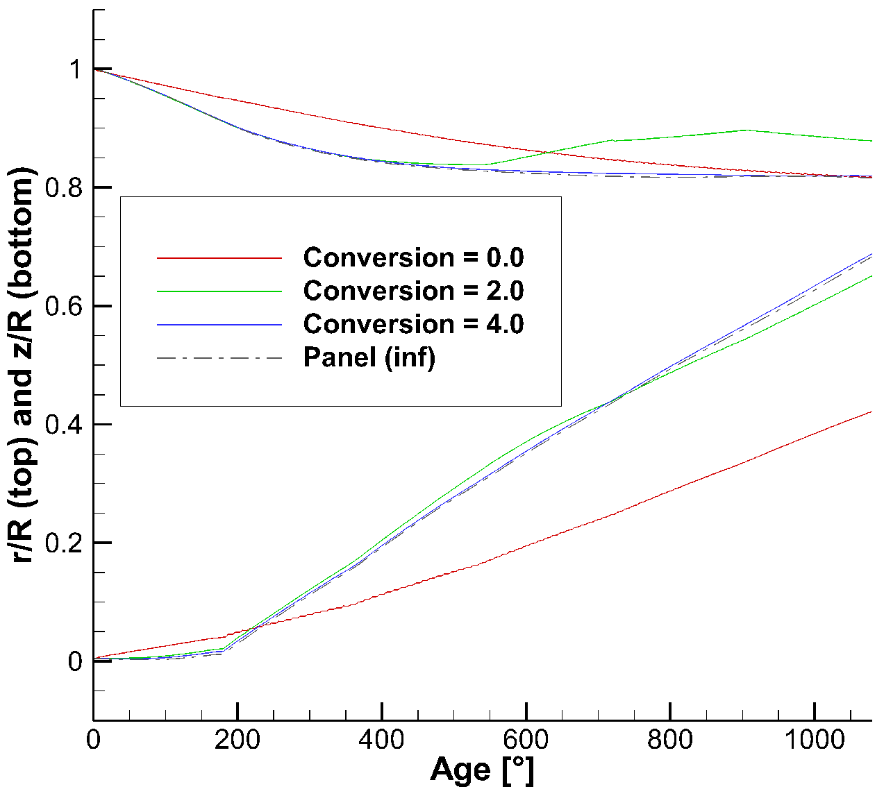
5.2.5. NL-UVLM-VPM Wake-Particle Conversion Revolution
5.2.6. Summary of the UVLM-VPM Parametrization
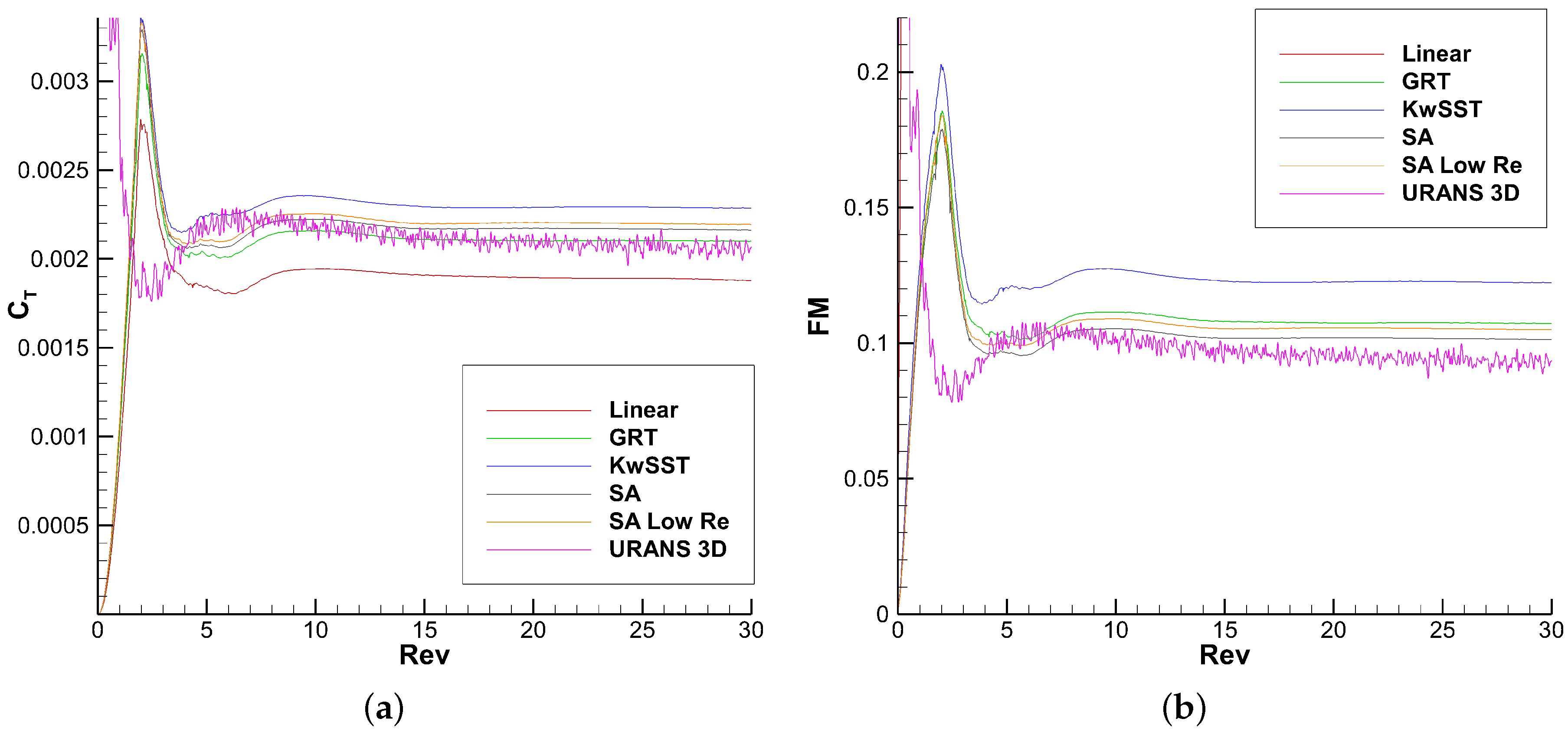
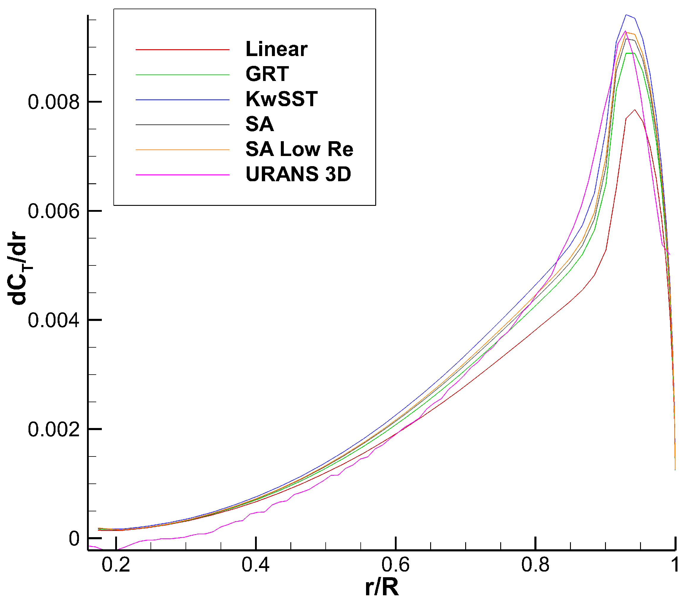
6. Results
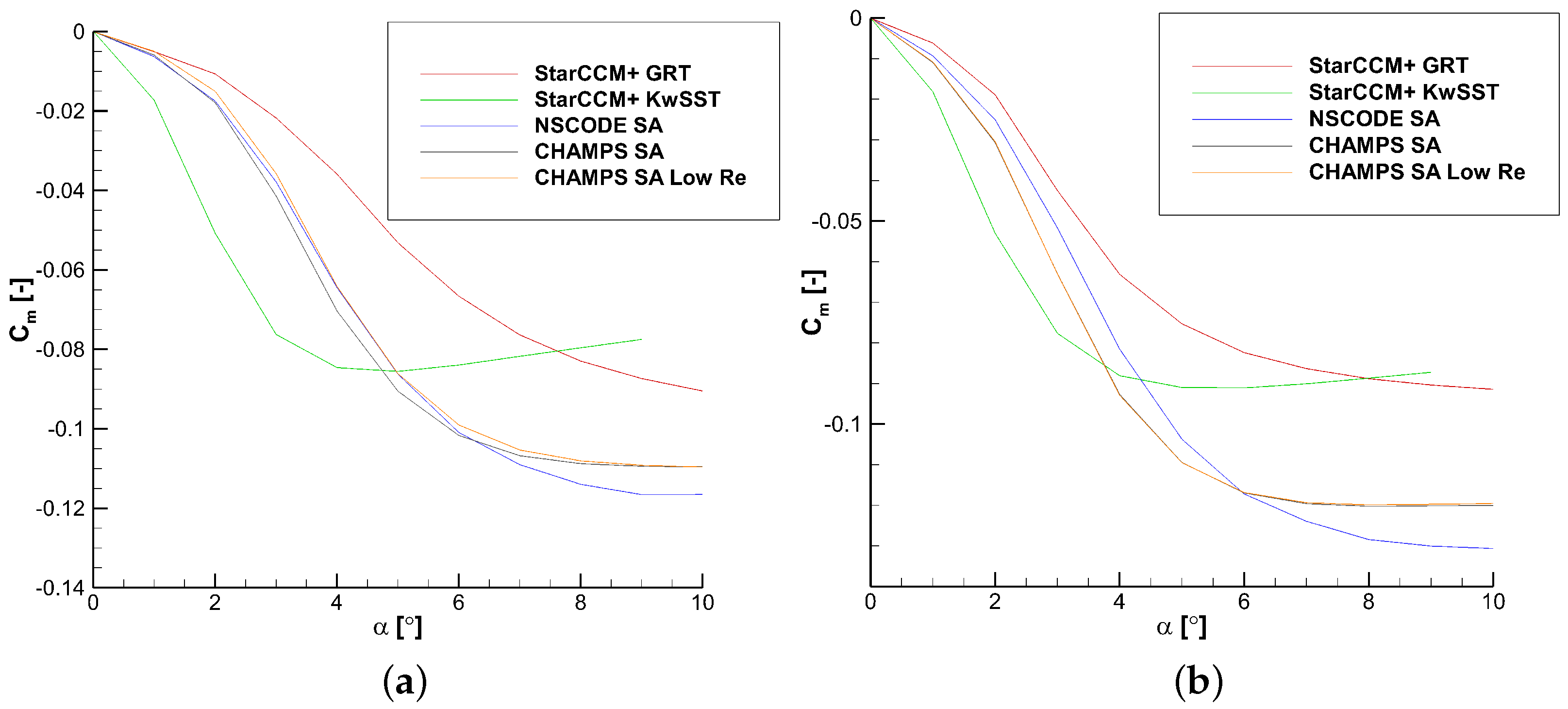
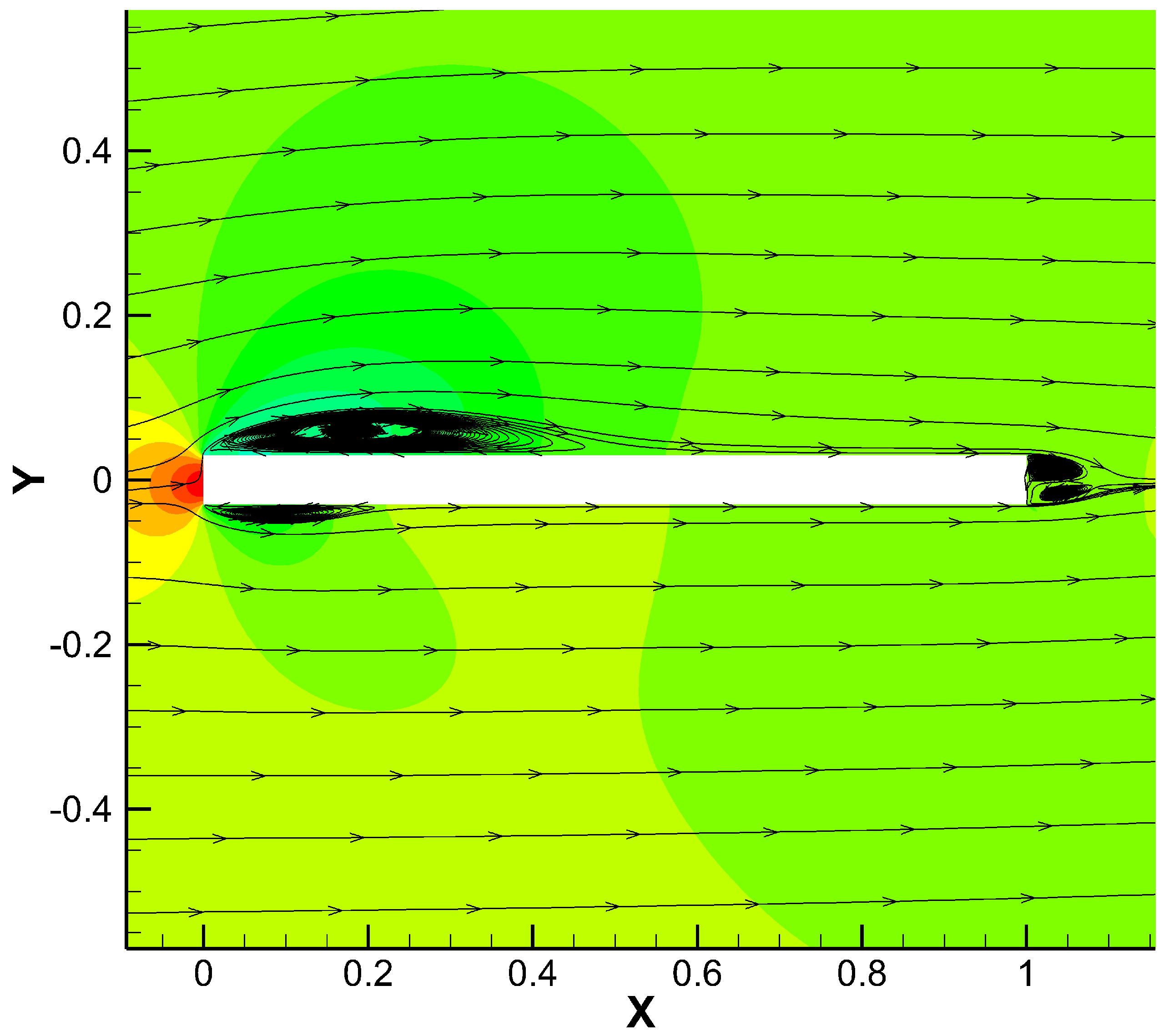
6.1. URANS 3D
6.2. NL-UVLM-VPM and URANS 3D Comparison
7. Conclusions
Author Contributions
Funding
Data Availability Statement
Acknowledgments
Conflicts of Interest
Appendix A. Database Generation


Appendix B. URANS 3D Refinement Study


| Name | Cell Count (M) | (°) | (%) | (%) | (%) | (%) |
|---|---|---|---|---|---|---|
| Mesh 1 | 7.0 | 2 | 1.06 | 0.59% | 1.53 | −9.05% |
| Mesh 2 | 11.1 | 2 | 1.30 | −1.71% | 1.89 | −11.26% |
| Mesh 3 | 20.6 | 2 | 1.31 | 1.89% | 1.88 | −0.38% |
| Mesh 4 | 38.0 | 2 | 1.31 | 1.38% | 1.89 | 0.02% |
| Mesh 5 | 65.3 | 2 | 1.40 | - | 2.01 | - |
| Time 1 | 20.6 | 8 | 0.81 | −5.86% | 1.17 | −6.85% |
| Time 2 | 20.6 | 4 | 1.48 | 0.81% | 2.14 | 1.48% |
| Time 3 | 20.6 | 2 | 1.31 | 1.76% | 1.88 | 2.50% |
| Time 4 | 20.6 | 1 | 1.32 | 1.91% | 1.89 | 2.61% |
| Time 5 | 20.6 | 0.5 | 1.50 | - | 2.16 | - |


References
- Leishman, G.J. Rotorcraft Aeromechanics: Getting through the Dip. J. Am. Helicopter Soc. 2010, 55, 11001. [Google Scholar]
- van Dam, C.P. The aerodynamic design of multi-element high-lift systems for transport airplanes. Prog. Aerosp. Sci. 2002, 38, 101–144. [Google Scholar] [CrossRef]
- Gallay, S.; Laurendeau, E. Nonlinear Generalized Lifting-Line Coupling Algorithms for Pre/Poststall Flows. AIAA J. 2015, 53, 1784–1792. [Google Scholar] [CrossRef]
- Jo, Y.; Jardin, T.; Gojon, R.; Jacob, M.C.; Moschetta, J.M. Prediction of noise from low Reynolds number rotors with different number of blades using a non-linear vortex lattice method. In Proceedings of the 25th AIAA/CEAS Aeroacoustics Conference, Delft, The Netherlands, 20–23 May 2019. [Google Scholar] [CrossRef]
- Proulx-Cabana, V.; Nguyen, M.T.; Prothin, S.; Michon, G.; Laurendeau, E. A Hybrid Non-Linear Unsteady Vortex Lattice-Vortex Particle Method for Rotor Blades Aerodynamic Simulations. Fluids 2022, 7, 81. [Google Scholar] [CrossRef]
- Vreman, A.W. An eddy-viscosity subgrid-scale model for turbulent shear flow: Algebraic theory and applications. Phys. Fluids 2004, 16, 3670–3681. [Google Scholar] [CrossRef]
- Johnson, W. Helicopter Theory, revised ed.; Dover Publications: New York, NY, USA, 1994. [Google Scholar]
- Hariharan, N.S.; Narducci, R.P.; Egolf, T.A. Helicopter Aerodynamic Modeling of S-76 Rotor with Tip-Shape Variations: Review of AIAA Standardized Hover Evaluations. In Proceedings of the 54th AIAA Aerospace Sciences Meeting, San Diego, CA, USA, 4–8 January 2016. [Google Scholar] [CrossRef]
- Colmenares, J.D.; López, O.D.; Preidikman, S. Computational Study of a Transverse Rotor Aircraft in Hover Using the Unsteady Vortex Lattice Method. Math. Probl. Eng. 2015, 2015, 478457. [Google Scholar] [CrossRef]
- Pérez, A.M.; Lopez, O.; Poroseva, S.V. Free-Vortex Wake and CFD Simulation of a Small Rotor for a Quadcopter at Hover. In Proceedings of the AIAA Scitech 2019 Forum, San Diego, CA, USA, 7–11 January 2019. [Google Scholar] [CrossRef]
- Alvarez, E.J.; Ning, A. Modeling multirotor aerodynamic interactions through the vortex particle method. In Proceedings of the AIAA Aviation 2019 Forum, Dallas, TX, USA, 17–21 June 2019. [Google Scholar] [CrossRef]
- Yücekayalı, A. Noise Minimal & Green Trajectory and Flight Profile Optimization for Helicopters. Ph.D. Thesis, Middle East Technical University, Ankara, Turkey, 2020. [Google Scholar]
- Zhao, J.; He, C. A Viscous Vortex Particle Model for Rotor Wake and Interference Analysis. J. Am. Helicopter Soc. 2010, 55, 12007. [Google Scholar] [CrossRef]
- Singh, P.; Friedmann, P.P. Application of Vortex Methods to Coaxial Rotor Wake and Load Calculations. In Proceedings of the 55th AIAA Aerospace Sciences Meeting, Grapevine, TX, USA, 9–13 January 2017. [Google Scholar] [CrossRef]
- Ferlisi, C. Rotor Wake Modelling Using the Vortex-Lattice Method. Master’s Thesis, École Polytechnique de Montréal, Montreal, QC, Canada, 2018. [Google Scholar]
- Tan, J.; Wang, H. Simulating unsteady aerodynamics of helicopter rotor with panel/viscous vortex particle method. Aerosp. Sci. Technol. 2013, 30, 255–268. [Google Scholar] [CrossRef]
- Tugnoli, M.; Montagnani, D.; Syal, M.; Droandi, G.; Zanotti, A. Mid-fidelity approach to aerodynamic simulations of unconventional VTOL aircraft configurations. Aerosp. Sci. Technol. 2021, 115, 106804. [Google Scholar]
- Samad, A.; Tagawa, G.; Morency, F.; Volat, C. Predicting rotor heat transfer using the viscous blade element momentum theory and unsteady vortex lattice method. Aerospace 2020, 7, 90. [Google Scholar] [CrossRef]
- Lee, H.; Sengupta, B.; Araghizadeh, M.S.; Myong, R.S. Review of vortex methods for rotor aerodynamics and wake dynamics. Adv. Aerodyn. 2022, 4, 20. [Google Scholar]
- Chattot, J.J. Analysis and design of wings and wing/winglet combinations at low speeds. In Proceedings of the 42nd AIAA Aerospace Sciences Meeting and Exhibit, Reno, NV, USA, 5–8 January 2004. [Google Scholar] [CrossRef]
- Caradonna, F.X.; Tung, C. Experimental and Analytical Studies of a Model Helicopter Rotor in Hover; National Aeronautics and Space Administration; US Army Aviation Research and Development Command: Washington, DC, USA; St. Louis, MO, USA, 1981.
- Harrington, R.D. Full-Scale-Tunnel Investigation of the Static-Thrust Performance of a Coaxial Helicopter Rotor; Technical Report TN 2318; NACA: Washington, DC, USA, 1951.
- Boatwright, D.W. Measurements of Velocity Components in the Wake of a Full-Scale Helicopter Rotor in Hover; Technical Report 72–33; USAAMRDL: Washington, DC, USA, 1972.
- Shinoda, P.M. Full-Scale S-76 Rotor Performance and Loads at Low Speeds in the NASA Ames 80-by 120-Foot Wind Tunnel; Technical Report 110379; NASA: Washington, DC, USA, 1996; Volume 2.
- Droandi, G.; Zanotti, A.; Gibertini, G. Aerodynamic interaction between rotor and tilting wing in hovering flight condition. J. Am. Helicopter Soc. 2015, 60, 042011. [Google Scholar]
- Zawodny, N.S.; Boyd, D.D., Jr.; Burley, C.L. Acoustic characterization and prediction of representative, small-scale rotary-wing unmanned aircraft system components. In Proceedings of the American Helicopter Society (AHS) Annual Forum, West Palm Beach, FL, USA, 17–19 May 2016. NF1676L-22587. [Google Scholar]
- Zhou, W.; Ning, Z.; Li, H.; Hu, H. An experimental investigation on rotor-to-rotor interactions of small UAV propellers. In Proceedings of the 35th AIAA Applied Aerodynamics Conference, Denver, CO, USA, 5–9 June 2017. [Google Scholar]
- Balch, D.T.; Lombardi, J. Experimental Study of Main Rotor Tip Geometry and Tail Rotor Interactions in Hover. Volume 1. Text and Figures; Technical Report 19850014034; NASA, Ames Research Center: Mountain View, CA, USA, 1985.
- Balch, D.T.; Lombardi, J. Experimental Study of Main Rotor Tip Geometry and Tail Rotor Interactions in Hover. Volume 2. Run Log and Tabulated Data; Technical Report 19850014035; NASA, Ames Research Center: Mountain View, CA, USA, 1985.
- Kocurek, J.D.; Tangler, J.L. A prescribed wake lifting surface hover performance analysis. J. Am. Helicopter Soc. 1977, 22, 24–35. [Google Scholar]
- Katz, J.; Plotkin, A. Low-Speed Aerodynamics, 2nd ed.; Cambridge Aerospace Series; Cambridge University Press: Cambridge, UK, 2001. [Google Scholar]
- Vatistas, G.H.; Kozel, V.; Mih, W.C. A simpler model for concentrated vortices. Exp. Fluids 1991, 11, 73–76. [Google Scholar] [CrossRef]
- Winckelmans, G.S. Topics in Vortex Methods for the Computation of Three-and Two-Dimensional Incompressible Unsteady Flows. Ph.D. Thesis, California Institute of Technology, Pasadena, CA, USA, 1989. [Google Scholar]
- Winckelmans, G.S.; Leonard, A. Contributions to Vortex Particle Methods for the Computation of Three-Dimensional Incompressible Unsteady Flows. J. Comput. Phys. 1993, 109, 247–273. [Google Scholar] [CrossRef]
- Tan, J.F.; Sun, Y.M.; Zhou, T.Y.; Barakos, G.N.; Green, R.B. Simulation of the aerodynamic interaction between rotor and ground obstacle using vortex method. CEAS Aeronaut. J. 2019, 10, 733–753. [Google Scholar] [CrossRef]
- Tan, J.F.; Sun, Y.M.; Barakos, G.N. Vortex approach for downwash and outwash of tandem rotors in ground effect. J. Aircr. 2018, 55, 2491–2509. [Google Scholar] [CrossRef]
- Greengard, L.; Rokhlin, V. A fast algorithm for particle simulations. J. Comput. Phys. 1987, 73, 325–348. [Google Scholar] [CrossRef]
- Barba, L.A.; Leonard, A.; Allen, C.B. Advances in viscous vortex methods—Meshless spatial adaption based on radial basis function interpolation. Int. J. Numer. Methods Fluids 2005, 47, 387–421. [Google Scholar]
- Degond, P.; Mas-Gallic, S. The weighted particle method for convection-diffusion equations. I. The case of an isotropic viscosity. Math. Comput. 1989, 53, 485–507. [Google Scholar] [CrossRef]
- Winckelmans, G.S. Some Progress in Large-Eddy Simulation Using the 3-D Vortex Particle Method; Technical Report 19960022324; Center for Turbulence Research Annual Research Briefs: New York, NY, USA, 1995. [Google Scholar]
- Winckelmans, G.; Cocle, R.; Dufresne, L.; Capart, R. Vortex methods and their application to trailing wake vortex simulations. Comptes Rendus Phys. 2005, 6, 467–486. [Google Scholar] [CrossRef]
- Gallay, S. Algorithmes de Couplage RANS et Écoulement Potentiel. Ph.D. Thesis, École Polytechnique de Montréal, Montréal, QC, Canada, 2016. [Google Scholar]
- Bourgault-Côté, S.; Ghasemi, S.; Mosahebi, A.; Laurendeau, E. Extension of a Two-Dimensional Navier–Stokes Solver for Infinite Swept Flow. AIAA J. 2017, 55, 662–667. [Google Scholar] [CrossRef]
- Parenteau, M.; Sermeus, K.; Laurendeau, E. VLM coupled with 2.5 d RANS sectional data for high-lift design. In Proceedings of the 2018 AIAA Aerospace Sciences Meeting, Kissimmee, FL, USA, 8–12 January 2018. [Google Scholar] [CrossRef]
- Menter, F.R. Two-equation eddy-viscosity turbulence models for engineering applications. AIAA J. 1994, 32, 1598–1605. [Google Scholar]
- Menter, F.R.; Langtry, R.; Völker, S. Transition modelling for general purpose CFD codes. Flow Turbul. Combust. 2006, 77, 277–303. [Google Scholar]
- Carreño Ruiz, M.; D’Ambrosio, D. Validation of the gamma-Re theta Transition Model for Airfoils Operating in the Very Low Reynolds Number Regime. Flow Turbul. Combust. 2022, 109, 279–308. [Google Scholar]
- Spalart, P.; Allmaras, S. A one-equation turbulence model for aerodynamic flows. In Proceedings of the 30th Aerospace Sciences Meeting and Exhibit, Reno, NV, USA, 6–9 January 1992. [Google Scholar] [CrossRef]
- Spalart, P.R.; Garbaruk, A.V. Correction to the Spalart–Allmaras Turbulence Model, Providing More Accurate Skin Friction. AIAA J. 2020, 58, 1903–1905. [Google Scholar]
- Proulx-Cabana, V.; Laurendeau, E. Towards non-linear unsteady vortex lattice method (NL-UVLM) for rotary-wing aerodynamics. In Proceedings of the CASI AERO, Montreal, QC, Canada, 14–16 May 2019. [Google Scholar]
- Plante, F.; Gagnon, M.; Laurendeau, E. Recent Developments in the CHApel Multi-Physics Simulation Software. In Proceedings of the Chapel Implementers and Users Workshop (CHIUW), Virtual, 10 June 2022. [Google Scholar]
- Roberts, W.B. Calculation of laminar separation bubbles and their effect on airfoil performance. AIAA J. 1980, 18, 25–31. [Google Scholar]
- Schmidt, G.S.; Mueller, T.J. Analysis of low Reynolds number separation bubbles using semiempirical methods. AIAA J. 1989, 27, 993–1001. [Google Scholar]
- Gabriel, E.T.; Mueller, T.J. Low-aspect-ratio wing aerodynamics at low Reynolds number. AIAA J. 2004, 42, 865–873. [Google Scholar]


| Authors | Method | Compressibility | Viscosity | Mesh | (°) | Sensitivity | Convergence (Rev) |
|---|---|---|---|---|---|---|---|
| Colmenares et al. [9] | UVLM | No | No | 6 × 15 cos | 10? | No | 12 |
| Perez et al. [10] | 7 × 33 | 10 | 9 | ||||
| Alvarez and Ning [11] | VPM | Prandtl–Glauert | Lookup | 1 × 50 | 5 | No | 20 |
| Yucekayali [12] | No | 1 × 30 | 7.5 | No | 6 | ||
| Zhao and He [13] | LL-VPM | No need with look-up | Lookup | 1 × 50 | 3.75 | Downwash at fixed | No |
| Singh and Friedmann [14] | UVLM- VPM | Karman–Tsien | Sectional drag | 2 × 8 | 12 | Not shown | 6 |
| Ferlisi [15] | No | No | 4 × 15? cos | 10 | No | 10 | |
| Tan and Wang [16] | UPM-VPM | No | No | 60 × 20 | 5 | No on hover | 10 |
| Tugnoli et al. [17] | NL-LL- VPM | No need with non-linear | Alpha or Gamma | 1 × 16 | 9 | Not shown | 20 |
| Samad et al. [18] | NL-UVLM | Prandtl–Glauert | Alpha | 10 × 25 | 15 | No | 24 |
| Jo et al. [4] | NL- UVLM- VPM | No need with non-linear | Gamma | 15 × 30 | 5 | and | 30 |
| Lee et al. [19] | 20 × 45? cos-cos | 5? | No | 20? | |||
| Previous work [5] | Alpha | 8 × 20 cos | 2.5 | and FM | 24 | ||
| Current work | Alpha | 16 × 40 cos | 10 | , FM, , and tip vortex | 28 |
| Validation | Exp. Year | RPM | Mach Tip | Reynolds | ||
|---|---|---|---|---|---|---|
| Harrington [22] | 1951 | 20.4 | 2 | 477 | 0.44 | M |
| 6.67 | 2 | 250 | 0.23 | M | ||
| 374 | 0.35 | M | ||||
| Boatwright [23] | 1972 | 16.2 | 2 | 245 | 0.40 | M |
| 340 | 0.56 | M | ||||
| Caradonna–Tung [21] | 1981 | 6.00 | 2 | 1250 | 0.44 | M |
| 1500 | 0.52 | M | ||||
| 1750 | 0.61 | M | ||||
| Hariharan et al. [8] | 1985 (2016) | 14.6 | 4 | 1484 | 0.60 | M |
| Shinoda [24] | 1996 | 14.6 | 4 | 293 | 0.60 | M |
| Droandi et al. [25] | 2015 | 5.50 | 4 | 1120 | 0.32 | k |
| Zawodny et al. [26] | 2016 | 6.67 | 2 | 5400 | 0.20 | k |
| Zhou et al. [27] | 2017 | 5.73 | 2 | 4860 | 0.18 | k |
| Perez et al. [10] | 2019 | 6.59 | 4 | 4500 | 0.25 | k |
| Present work | NA | 8.00 | 2 | 1000 | 0.15 | k |
| Authors | Validation | Validation Points | || (%) | || (%) | Trimmed | Span Load | Tip Vortex | Convergence Figure |
|---|---|---|---|---|---|---|---|---|
| Colmenares et al. [9] | Caradonna–Tung [21] | 3 | 6 | No | No | No | ||
| Perez et al. [10] | Perez et al. [10] | 1 | CFD: 8 Exp: 12 | CFD: 18 Exp: 5 | No | contour | No | and |
| Alvarez and Ning [11] | Zhou et al. [27] | 1 | 0.6 | No on hover | No | No | No | |
| Yucekayali [12] | Shinoda [24] and Caradonna–Tung [21] | 5 with [24] 1 with [21] | No | 7 † with [24] | Yes | with [21] | Yes | |
| Zhao and He [13] | Boatwright [23] and Caradonna–Tung [21] | 1 with each ref | No | No | Yes | with [21] | No | No |
| Singh and Friedmann [14] | Harrington [22] | 22 | No | [4–12] † | Yes | No | No | No |
| Ferlisi [15] | Caradonna–Tung [21] | 3 | 4 | No | No | No | Yes | |
| Tan and Wang [16] | Caradonna–Tung [21] * | 3 | No | No | No | sections | No | No |
| Tugnoli et al. [17] | Droandi et al. [25] | 11 | No | Exp: 9 † | Yes | No | No | |
| Samad et al. [18] | Caradonna–Tung [21] | 3 | 6 | No | No | No | ||
| Jo et al. [4] | Zawodny et al. [26] | 1 | CFD: 3.6 Exp: 0.4 | No | No | No | No | No |
| Lee et al. [19] | Caradonna–Tung [21] | 3 | Small | No | No | Yes | No | |
| Previous work [5] | Hariharan et al. [8] | 6 | CFD: 3 Exp: 8 | CFD: 2 † Exp: 5 † | Yes | and sections | No | and FM |
| Present work | Present work | 1 | [0.3–5.3] | [0.3–8.4] | No | , and | No | and FM |
| Property | Value |
|---|---|
| Number of Blades | 2 |
| Root cut-out ratio () | 15.79% |
| Radius | 475 [mm] |
| Twist | No |
| Taper | No |
| Chord | 50 [mm] |
| Profile | Rectangle |
| Thickness | 3 [mm] |
| Rotational velocity () | 1000 [RPM] |
| Collective angle () | 5 [°] |
| Reynolds number (root–tip) | 26,884–170,263 |
| Mach number (root–tip) | 0.02–0.15 |
| Software | Flow Solver | Mesh | Turbulence Model |
|---|---|---|---|
| StarCCM+ (Commerical) | 2D Steady Reynolds Averaged Navier–Stokes (RANS) Compressible coupled | 182 k elements (quad and hex) | SST [45] (KwSST) (Fully turbulent) |
| KwSST- [46,47] (GRT) (Transitional) | |||
| CHAMPS (In-house) | 92 k elements (quad) | Spalart–Allmaras [48] (SA) (Fully turbulent) | |
| SA Low-Reynolds [49] (SA Low Re) (Fully turbulent) | |||
| NSCODE (In-house) | Spalart–Allmaras [48] (SA) (Fully turbulent) |
| (%) | (%) | (%) | (%) | (%) | ||
|---|---|---|---|---|---|---|
| 20 | 1.97 | 0.43 | 2.86 | 8.35 | 0.72 | 3.29 |
| 40 | 1.91 | 0.42 | −0.31 | 8.08 | 0.62 | −0.10 |
| 60 | 1.92 | 0.24 | - | 8.09 | 0.25 | - |
| 80 | 1.80 | 0.34 | −6.04 | 7.82 | 0.14 | −3.37 |
| 100 | 1.81 | 0.09 | −5.78 | 7.67 | 0.14 | −5.13 |
| Mesh | (%) | (%) | (%) | (%) | ||
|---|---|---|---|---|---|---|
| 4 × 10 | 1.90 | 0.55 | 3.87 | 8.24 | 0.65 | −0.42 |
| 8 × 20 | 1.90 | 0.26 | 3.53 | 8.23 | 0.26 | −0.46 |
| 12 × 30 | 1.77 | 0.14 | −3.47 | 8.42 | 0.19 | 1.81 |
| 16 × 40 | 1.80 | 0.15 | −1.63 | 8.32 | 0.29 | 0.56 |
| 24 × 60 | 1.83 | 0.10 | 0.15 | 8.28 | 0.31 | 0.13 |
| 32 × 80 | 1.84 | 0.21 | 0.47 | 8.26 | 0.14 | −0.18 |
| 48 × 120 | 1.83 | 0.11 | - | 8.27 | 0.16 | - |
| (°) | (%) | (%) | (%) | (%) | ||
|---|---|---|---|---|---|---|
| 20 | 2.02 | 0.10 | −3.80 | 1.02 | 0.14 | −5.01 |
| 10 | 2.06 | 0.28 | −1.73 | 1.05 | 0.39 | −2.31 |
| 5 | 2.10 | 0.42 | - | 1.07 | 0.59 | - |
| (%) | (%) | (%) | (%) | (%) | ||
|---|---|---|---|---|---|---|
| 0 | 2.26 | 0.34 | 8.94 | 1.18 | 0.47 | 11.83 |
| 20 | 2.16 | 0.58 | 4.40 | 1.11 | 0.76 | 5.87 |
| 40 | 2.14 | 0.35 | 3.44 | 1.10 | 0.47 | 4.52 |
| 60 | 2.07 | 0.12 | - | 1.05 | 0.16 | - |
| 0.0 | 0.3 | 0.5 | 0.7 | 0.9 | 1.1 | 1.5 | 2.0 | >= 2.5 | |
| Instability (Rev) | 13 | 36 | 40 | 42 | 49 | 51 | 52 | 61 | >70 |
| (%) | (%) | (%) | (%) | |
|---|---|---|---|---|
| 2.5 | 0.11 | 0.10 | 0.14 | 2.94 |
| 2.8 | 0.12 | 0.08 | 0.14 | 2.91 |
| 3.0 | 0.10 | 0.32 | 0.11 | 3.14 |
| 3.5 | 0.10 | 0.65 | 0.11 | 3.47 |
| 5.0 | 0.08 | 1.04 | 0.10 | 3.82 |
| (%) | (%) | (%) | (%) | (%) | (%) | |
|---|---|---|---|---|---|---|
| 20 | 0.14 | −2.90 | −3.14 | 0.19 | −3.53 | −3.74 |
| 10 | 0.01 | 0.38 | 0.13 | 0.01 | 0.52 | 0.30 |
| 5 | 0.02 | 0.25 | −0.01 | 0.03 | 0.31 | 0.10 |
| 2.5 | 0.03 | - | −0.25 | 0.04 | - | −0.22 |
| Mesh | (%) | (%) | (%) | (%) |
|---|---|---|---|---|
| 4 × 10 | 0.03 | −0.06 | 0.04 | 0.03 |
| 8 × 20 | 0.02 | −0.32 | 0.02 | −0.48 |
| 16 × 40 | 0.01 | 0.12 | 0.01 | 0.15 |
| 24 × 60 | 0.02 | −0.05 | 0.02 | −0.07 |
| 32 × 80 | 0.02 | - | 0.02 | - |
| (%) | (%) | (%) | (%) | |
|---|---|---|---|---|
| 20 | 0.01 | −0.89 | 0.01 | −1.14 |
| 10 | 0.05 | - | 0.06 | - |
| (%) | (%) | (%) | (%) | |
|---|---|---|---|---|
| 20 | 0.06 | −2.18 | 0.07 | −2.83 |
| 10 | 0.02 | −1.07 | 0.02 | −1.40 |
| 5 | 0.03 | - | 0.04 | - |
| Conversion (Rev) | 0.0 | 0.5 | 1.0 | 2.0 | 4.0 | ∞ |
| Instability (Rev) | 34 | 12 | ∼25 | >42 | >32 | >48 |
| Conversion (Rev) | (%) | (%) | (%) | (%) |
|---|---|---|---|---|
| 0 | 0.09 | 2.38 | 0.12 | 2.95 |
| 2 | 0.03 | 1.13 | 0.04 | 1.61 |
| 4 | 0.06 | 0.42 | 0.09 | 0.63 |
| Panel (∞) | 0.24 | - | 0.32 | - |
| Viscous Database | (%) | (%) | (%) | (%) |
|---|---|---|---|---|
| Linear | 0.12 | −9.29 | 0.11 | 622 |
| GRT | 0.05 | 1.99 | 0.06 | 15.3 |
| KwSST | 0.03 | 11.0 | 0.04 | 31.3 |
| SA | 0.04 | 5.05 | 0.06 | 8.85 |
| SA Low Re | 0.03 | 6.54 | 0.04 | 12.7 |
| Viscous Database | (%) | (%) | (%) |
|---|---|---|---|
| Linear | −14.3 | −87.6 | 540 |
| GRT | −3.26 | −8.18 | 3.63 |
| KwSST | 5.32 | −8.39 | 18.0 |
| SA | −0.31 | 1.68 | −2.11 |
| SA Low Re | 1.12 | 0.26 | 1.43 |
Disclaimer/Publisher’s Note: The statements, opinions and data contained in all publications are solely those of the individual author(s) and contributor(s) and not of MDPI and/or the editor(s). MDPI and/or the editor(s) disclaim responsibility for any injury to people or property resulting from any ideas, methods, instructions or products referred to in the content. |
© 2024 by the authors. Licensee MDPI, Basel, Switzerland. This article is an open access article distributed under the terms and conditions of the Creative Commons Attribution (CC BY) license (https://creativecommons.org/licenses/by/4.0/).
Share and Cite
Proulx-Cabana, V.; Michon, G.; Laurendeau, E. Parametrization Effects of the Non-Linear Unsteady Vortex Method with Vortex Particle Method for Small Rotor Aerodynamics. Fluids 2024, 9, 24. https://0-doi-org.brum.beds.ac.uk/10.3390/fluids9010024
Proulx-Cabana V, Michon G, Laurendeau E. Parametrization Effects of the Non-Linear Unsteady Vortex Method with Vortex Particle Method for Small Rotor Aerodynamics. Fluids. 2024; 9(1):24. https://0-doi-org.brum.beds.ac.uk/10.3390/fluids9010024
Chicago/Turabian StyleProulx-Cabana, Vincent, Guilhem Michon, and Eric Laurendeau. 2024. "Parametrization Effects of the Non-Linear Unsteady Vortex Method with Vortex Particle Method for Small Rotor Aerodynamics" Fluids 9, no. 1: 24. https://0-doi-org.brum.beds.ac.uk/10.3390/fluids9010024