
The Influence of Two-Dimensional Temperature Modulation on Floating Droplet Dynamics
Department of Mathematics, Technion-Israel Institute of Technology, Haifa 32000, Israel
*
Author to whom correspondence should be addressed.
Fluids 2024, 9(1), 6; https://0-doi-org.brum.beds.ac.uk/10.3390/fluids9010006
Submission received: 20 October 2023
/
Revised: 13 December 2023
/
Accepted: 21 December 2023
/
Published: 25 December 2023
(This article belongs to the Topic Fluid Mechanics)
Abstract
:We investigate the dynamics and instabilities of a droplet that floats on a liquid substrate. The substrate is cooled from below. In the framework of the slender droplet approximation and the precursor model, the problem is studied numerically. Oscillatory and stationary regimes of thermocapillary convection have been observed. The influence of a two-dimensional spatial inhomogeneity of temperature on the droplet dynamics is investigated. The two-dimensional spatial temperature inhomogeneity can suppress oscillations, changing the droplet’s shape. In a definite region of parameters, the two-dimensional spatial modulation can lead to the excitation of periodic oscillations. The influence of the Biot number on the shape of the droplets is studied.
1. Introduction
The motion of a viscous liquid droplet on a solid substrate, which contradicts the nonslip condition, has been studied extensively during the past few decades [1,2]. The exploration of the dynamic phenomena (specifically, the difference between the static and dynamic contact angles and the existence of the dynamic contact angle hysteresis) led to essential progress in the understanding of interfacial phenomena.
Droplets on a liquid substrate (“liquid lenses”) are very important in various branches of engineering, including microfluidics [3], chemical engineering [4], environment protection [5], etc. Nevertheless, their dynamics has still attracted less attention.
The dynamics and instabilities of nonisothermal floating droplets are of special interest. Oscillatory convective motions, generated by the thermocapillary effect and buoyancy, have been observed in some experiments [6,7,8]. Recently, the influence of the homogeneous heating or cooling of the liquid substrate on the stability of a thin floating droplet under microgravity conditions has been studied in [9]. A number of instability modes leading to droplet oscillations, droplet decomposition or the substrate layer’s rupture were revealed. The observed instabilities of droplets are reminiscent of longwave deformational instabilities in two-layer films [10].
In various applications (e.g., in microfluidic devices), it can be necessary to move a droplet in a controllable way. The simplest way to influence the dynamics of a droplet is a temperature inhomogeneity that creates a thermocapillary motion. Typically, the droplet is advected by the thermocapillary flow in a liquid layer in the direction opposite to the surface temperature gradient, but there is a contribution to the droplet velocity due to the thermocapillary stresses on the droplet interfaces and due to the shear in the substrate liquid [11]. The direction of motion can be different depending on the details of the generated convective flow [6] and the droplet shape [12]. Moreover, the direction of the flow can change periodically with time due to the laser heating of a droplet [6,7]. Experiments on droplet evaporation where the buoyancy–thermocapillary convection caused by the evaporative cooling creates hydrothermal waves [8] and leads to the droplet disintegration [13] can also be mentioned.
In the present work, the dynamics of a droplet on a liquid substrate cooled from below under the action of a two-dimensional spatial temperature modulation is studied. The results of numerical simulations carried out in the framework of the longwave approximation and the precursor model are presented. The novelty of the present investigation is as follows. We show that a two-dimensional spatial temperature modulation can significantly change the shape of the droplet and oscillation features. Specifically, the two-dimensional spatial inhomogeneity of the temperature can suppress oscillations, leading to the formation of steady droplets. In a definite region of parameters, the two-dimensional spatial modulation can lead to the excitation of the specific type of periodic oscillations. For the first time, the influence of the Biot number on the shape of the droplet is studied.
The structure of this paper is as follows. We give the formulation of the problem in Section 2. The action of the two-dimensional spatial modulation of temperature on nonlinear stationary droplets is considered in Section 3. Droplet oscillations generated by an oscillatory thermocapillary instability in the presence of two-dimensional temperature modulation are described in Section 4. The influence of gravity on the droplet dynamics is discussed in Section 5. The influence of the Biot number on the shape of droplets is considered in Section 6. Some concluding remarks are presented in Section 7.
2. Formulation of the Problem
We consider a droplet of liquid 2 that floats on the layer of liquid 1, and both are in contact with the gas phase 3 (see Figure 1). Later on, we do not consider any processes in fluid 3: at the gas/liquid interface, the viscous stresses are neglected. The heat transfer is described using the heat exchange coefficient q. The mth fluid has density , dynamic viscosity and thermal conductivity , .
The contact angles on the triple line surrounding the droplet are determined by the balance of interfacial tensions , and between the corresponding fluids according to the Neumann triangle construction [14]. The droplet exists in two cases: (i) when the spreading coefficient (partial wetting); (ii) when but only a small part of fluid 2 is spread between fluids 1 and 3 forming an ultrathin film (pseudo-partial wetting) due to the attractive interaction of those fluids through the film of fluid 2 (positive Hamaker constant A).
In the present paper, we consider the thermocapillary convection in a floating droplet. The temperature of the gas phase is , and the temperature of the solid substrate is a function of horizontal coordinates, . Assuming that the temperature differences in the system are not too large, we disregard the dependence of liquid parameters on the temperature, with only one exception: because we are interested in the investigation of the thermocapillary convection, we take into account the thermocapillary stresses proportional to derivatives of the interfacial tensions with respect to the temperature. The interfacial tension coefficients on the lower and upper surfaces of the droplet, and , are assumed to be linear functions of temperature T: and , where and are constants. It is assumed that and ; therefore, we disregard that dependence in the relations that contain the interfacial tensions as a whole, i.e., in the stress balances on the triple line and in the expressions for Laplace pressures.
The description of the temporal evolution of the triple line surrounding the droplet is technically difficult (see [15]). In [16], the precursor model was suggested for the description of a floating droplet: the interface between fluids 1 and 3 outside the droplet is replaced by an ultrathin precursor layer of fluid 2 (see Figure 1). The latter model describes the droplet on the liquid substrate as a two-layer film. The same equations are used in the whole region, but outside the droplet, where the top layer is ultrathin, the corresponding disjoining pressure is taken into account. Let us emphasize that the latter approach can be applied both in the case of pseudo-partial wetting and partial wetting, because macroscopically both cases are identical. In the present paper, we apply that approach for the description of the dynamics of a nonisothermal floating droplet.
Far from the droplet, the equilibrium thickness of layer 1 is , and the thickness of the precursor film is . The deformable interfaces are described by equations and . The gravity acceleration is g.
Later on, we consider a slender droplet, i.e., where the slopes of both droplet’s interfaces are small. Also, we assume that the characteristic horizontal scale of the interface deformations is large as compared to the characteristic vertical size of the droplet and the substrate. Those assumptions allow us to apply the mathematical model governing the longwave dynamics of nonisothermal liquid layers that has been derived using the lubrication approximation [17] (see also [10,18,19]). In the framework of the longwave approach, the shapes of the interfaces and depend on the scaled horizontal coordinates and , , rather than on x and y. Also, it is assumed that they depend on the scaled time variable . A comprehensive description of the longwave approach can be found in the review paper [20].
We present the problem in the nondimensional form using the equilibrium thickness of the lower layer, as the vertical length scale. The choice of the horizontal scale is arbitrary [19]. We choose
as a time scale and
as a pressure scale.
The nondimensional parameters of the problem are as follows. We define the local Marangoni number as
which is a function of X and Y rather than a number. Also, we shall use the mean Marangoni number
where is a characteristic mean temperature of the substrate.
The other nondimensional parameters of the problem are defined as follows:
is the Biot number, , , , and .
In the framework of the lubrication approximation, the velocity and pressure fields are enslaved to the deformations of interfaces. The temporal evolution of those deformations is governed by the volume conservation equations [18]:
where , and .
The expressions for pressures,
include the contributions of the Laplacian pressures, hydrostatic pressures and disjoining pressures. Because the thickness of liquid layer 1 is always macroscopic, we can neglect the contribution of . In layer 2, we apply the following expression for the disjoining pressure:
where a is the nondimensional Hamaker constant, which is related to the dimensional Hamaker constant A as follows:
and (for details, see [16,21]).
The expressions for mobilities , , are
The nondimensional expressions for the rates of the thermocapillary flows are
where
Note that in the absence of gravity, a liquid layer with a deformable interface is subject to a monotonic Marangoni instability for arbitrary , i.e., by any heating from below [22]. That instability is not saturable, and it leads to the rupture of the substrate layer. The temperature disturbance caused by the droplet acts as “a seed” of instability. Therefore, in the presence of the temperature gradient, one can expect the existence of a stable configuration containing a droplet on a layer flat on the infinity only if , i.e., by cooling from below.
In the present work, we consider nonlinear regimes of the thermocapillary convection in the case of a spatially periodic temperature modulation of the local Marangoni number,
where , , , and . Note that the change in the sign of or is obtained by a translation or , correspondingly. Because of the symmetry of the problem with respect to the transformations and , it is sufficient to consider the case .
The problem governed by Equations (6)–(10) and (12)–(15) has been solved numerically with some initial conditions. The evolution equations were discretized using central differences for spatial derivatives and solved using an explicit scheme. Periodic boundary conditions have been applied on the boundaries of the computational region .
The computations have been performed in the region using the grid . Some additional simulations on the grids and did not reveal any qualitative changes.
Computations have been performed for the system of fluorinert FC70 (liquid 1) and silicon oil 10 (liquid 2). This system was used in microgravity experiments (see, e.g., [23]). We applied the following set of liquid parameters that was formerly used in simulations of the thermocapillary instability in two-layer systems [19]: , , , , . , , , , and . The value of is chosen equal to (see [9]).
3. Manipulation by a Stationary Droplet
In this section, we describe the shape of a stationary droplet in the limit of large .
3.1. The Case of Axisymmetric Initial Conditions
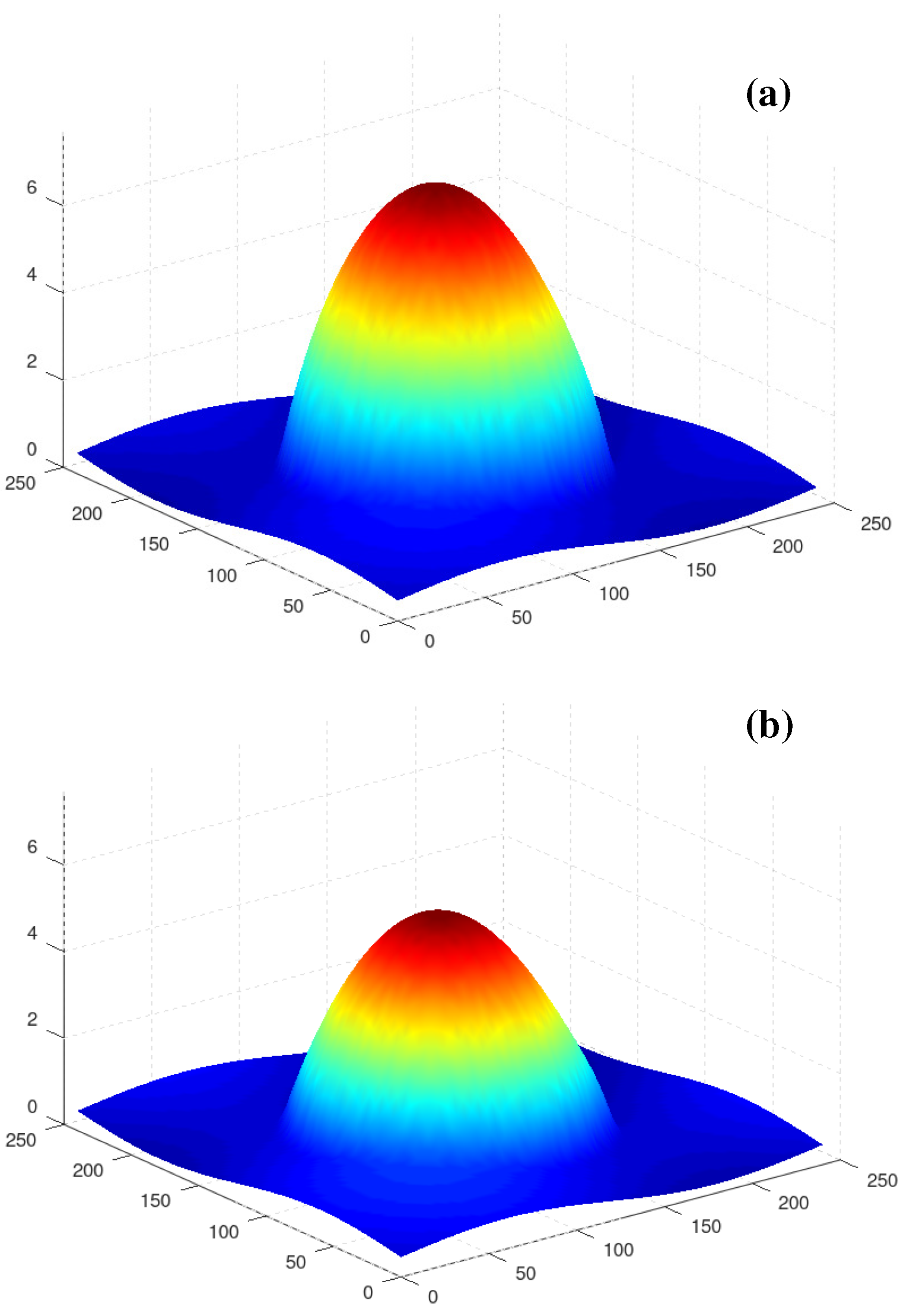
It is known that in the absence of gravity and the thermocapillary effect, both interfaces of an equilibrium droplet are spherical caps. The exact formulas that follow from the balance of interfacial tensions on the triple line are given in [24]. In the longwave limit, these interfaces become paraboloids with constant values of and , where r is the radial coordinate. When a temperature gradient across the substrate layer is applied, the temperature on both droplet interfaces becomes inhomogeneous; therefore, the thermocapillary convection is developed both in the droplet and in the substrate. If the initial conditions with an axisymmetric drop shape are applied and , for sufficiently small values of the droplet is stationary and axisymmetric in the limit . The shapes of isolines for and , which are determined by equations and , look perfectly circular, despite the violation of the rotational symmetry by the periodic boundary conditions [9]. Note that in contradistinction to the case of an isothermal droplet, both and are negative, except the vicinity of the triple line. Indeed, when the terms and caused by the inhomogeneities of the interfacial temperatures are dominant in the expressions (7) for flow rates, the system tends to minimize those inhomogeneities. The temperature of the interface between the substrate and the droplet is nearly constant when the ratio is nearly constant.
Let us take the steady round droplet [9] (; ) as the initial condition and consider its evolution under the action of two-dimensional temperature modulation (; ). In the case , the Marangoni number field (15) can be written as
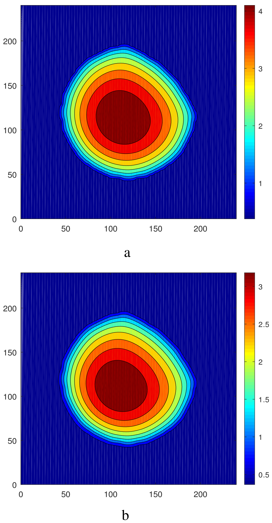
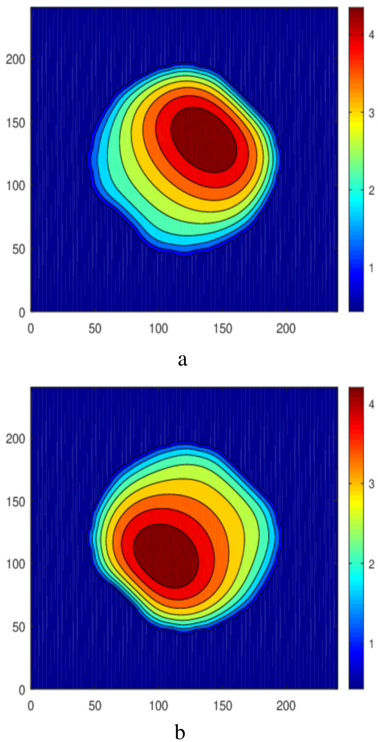
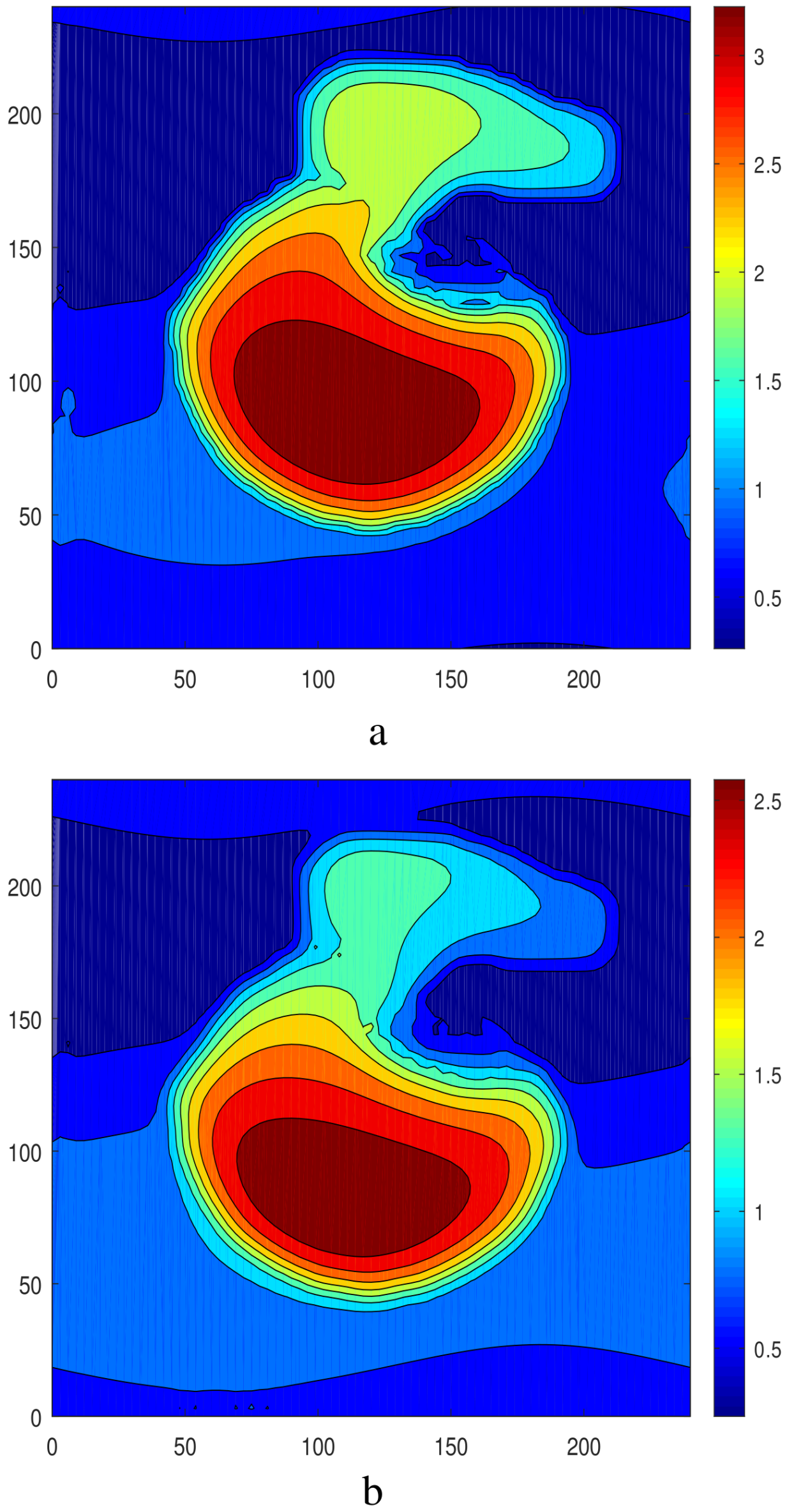
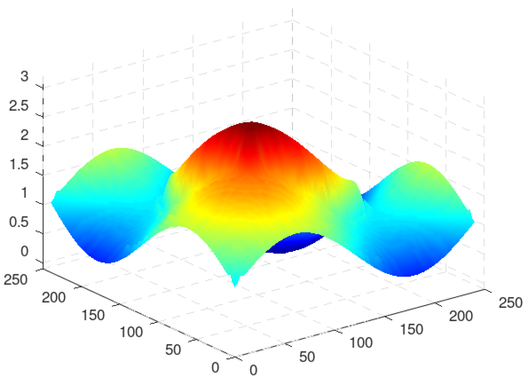
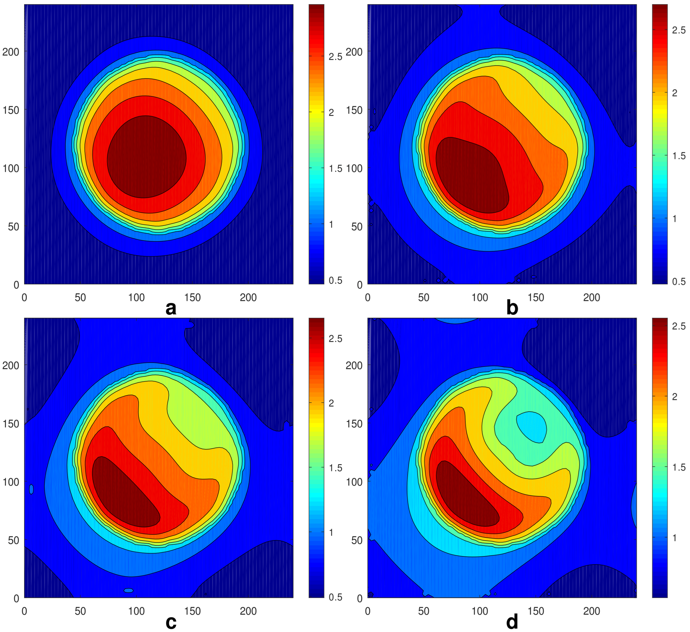
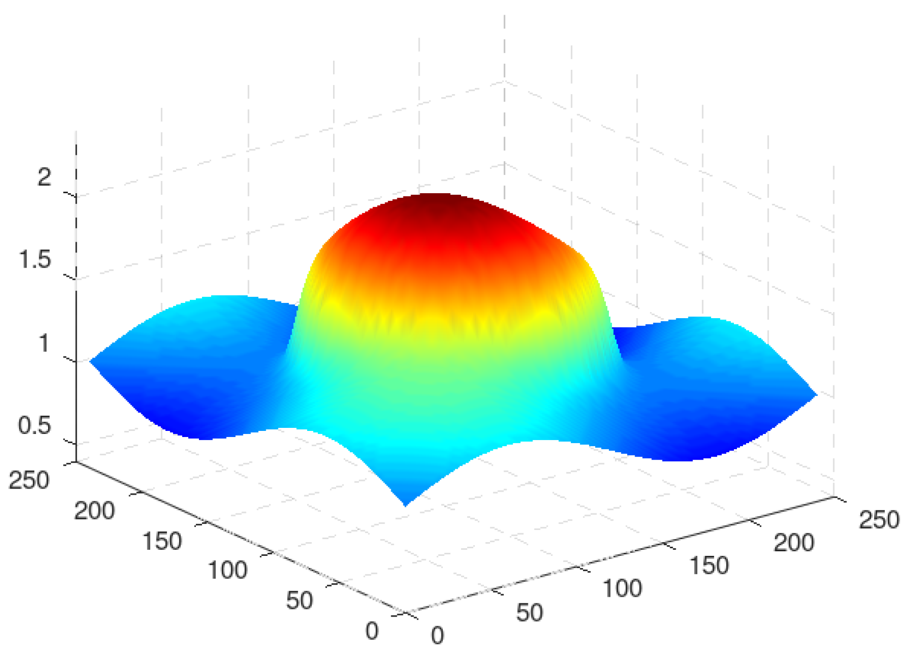
Thus, the substrate temperature inhomogeneity has the shape of a square pattern. The function is symmetric with respect to axes , , and . It changes its sign on the lines and . Near the diagonal , it is negative for and positive for . Under the action of the thermocapillary stresses, the liquid in the droplet moves slowly towards the region , , changing its shape and height. The intermediate stages of the evolution of the initially round droplet are presented in Figure 2. A change in the droplet’s shape is visible between Figure 2a,c. At 200,000, the equilibration takes place. Finally, we obtain the steady droplet with the maximum, shifted along the axis to the region , where the local value of is higher (i.e., into the cooler part of the region). Figure 3 shows a snapshot of the fields of (a) and (b) at the equilibrium stage. The droplet is not round anymore, but it keeps the symmetry with respect to the axis .
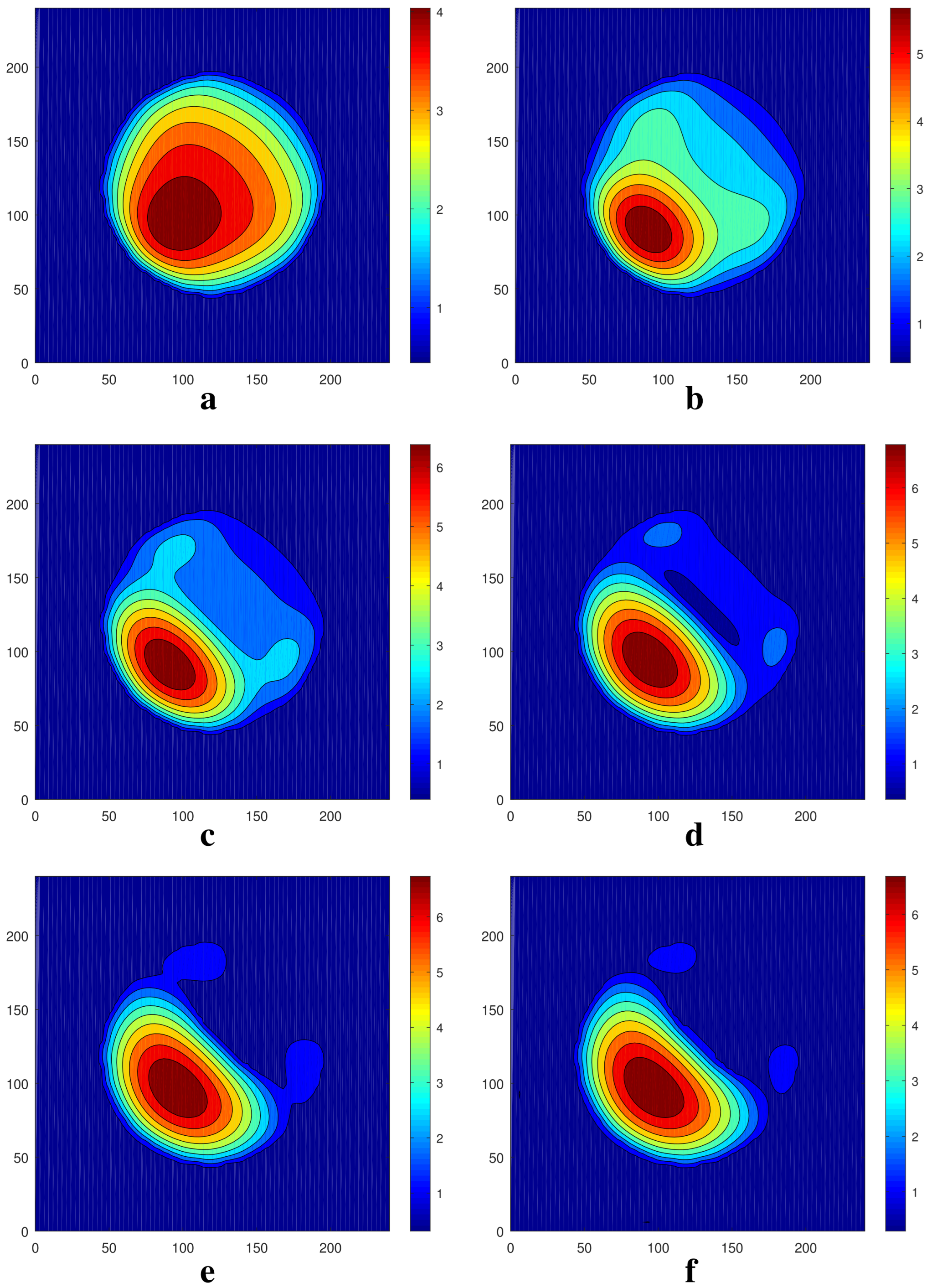
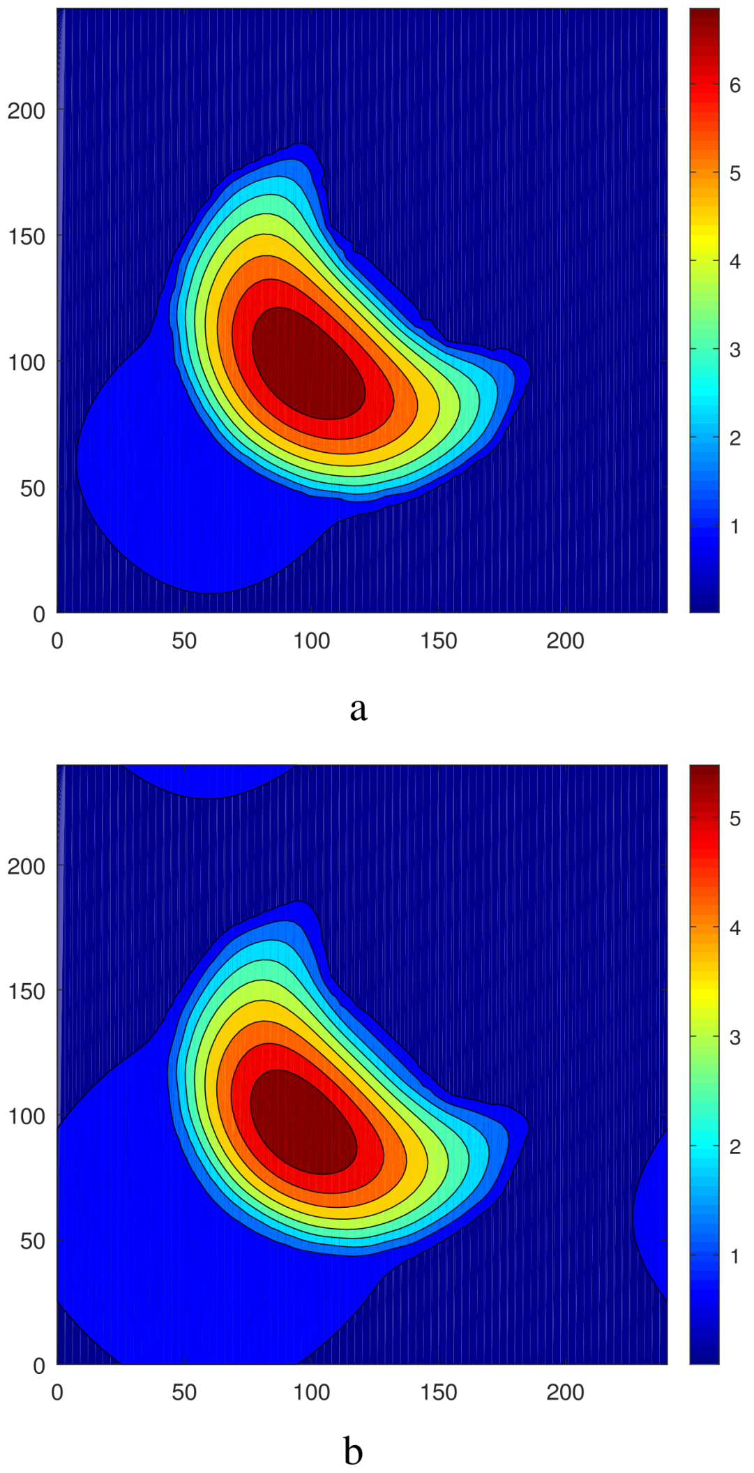
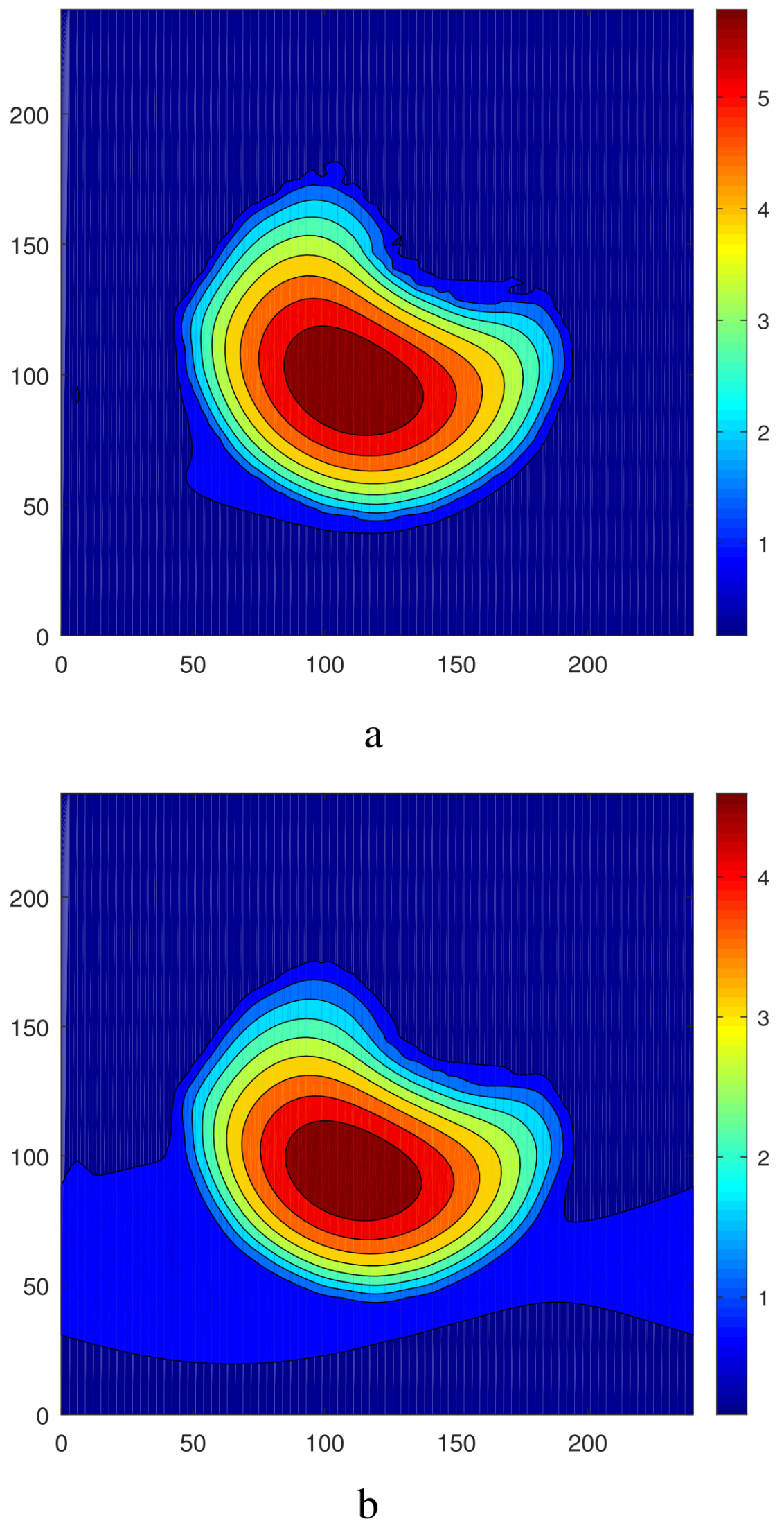
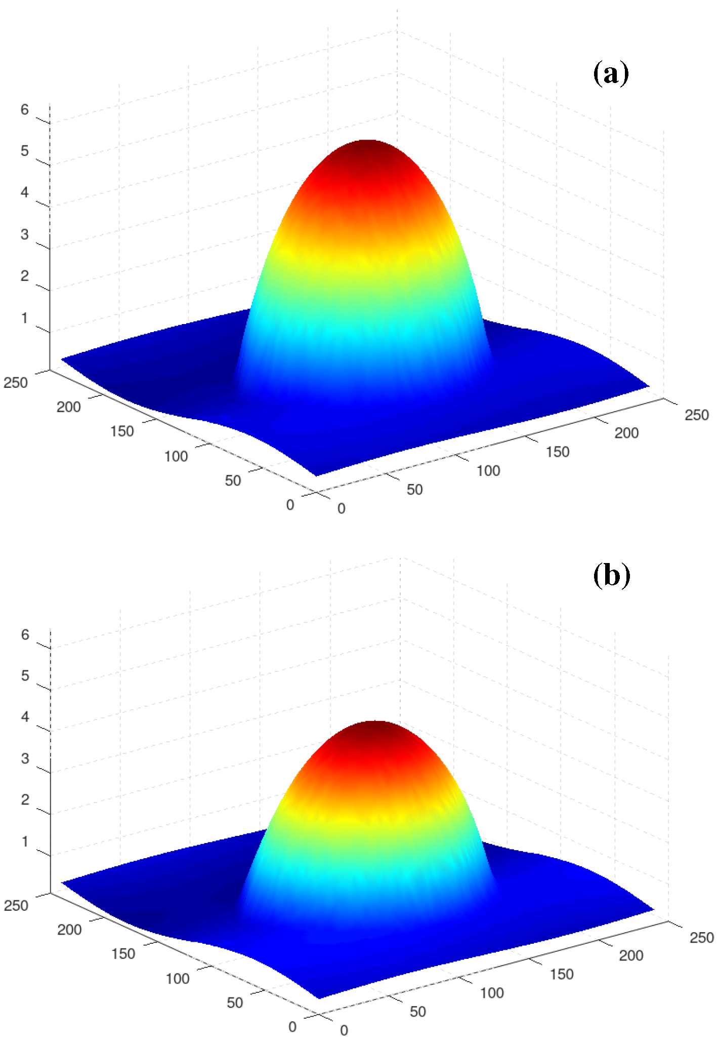
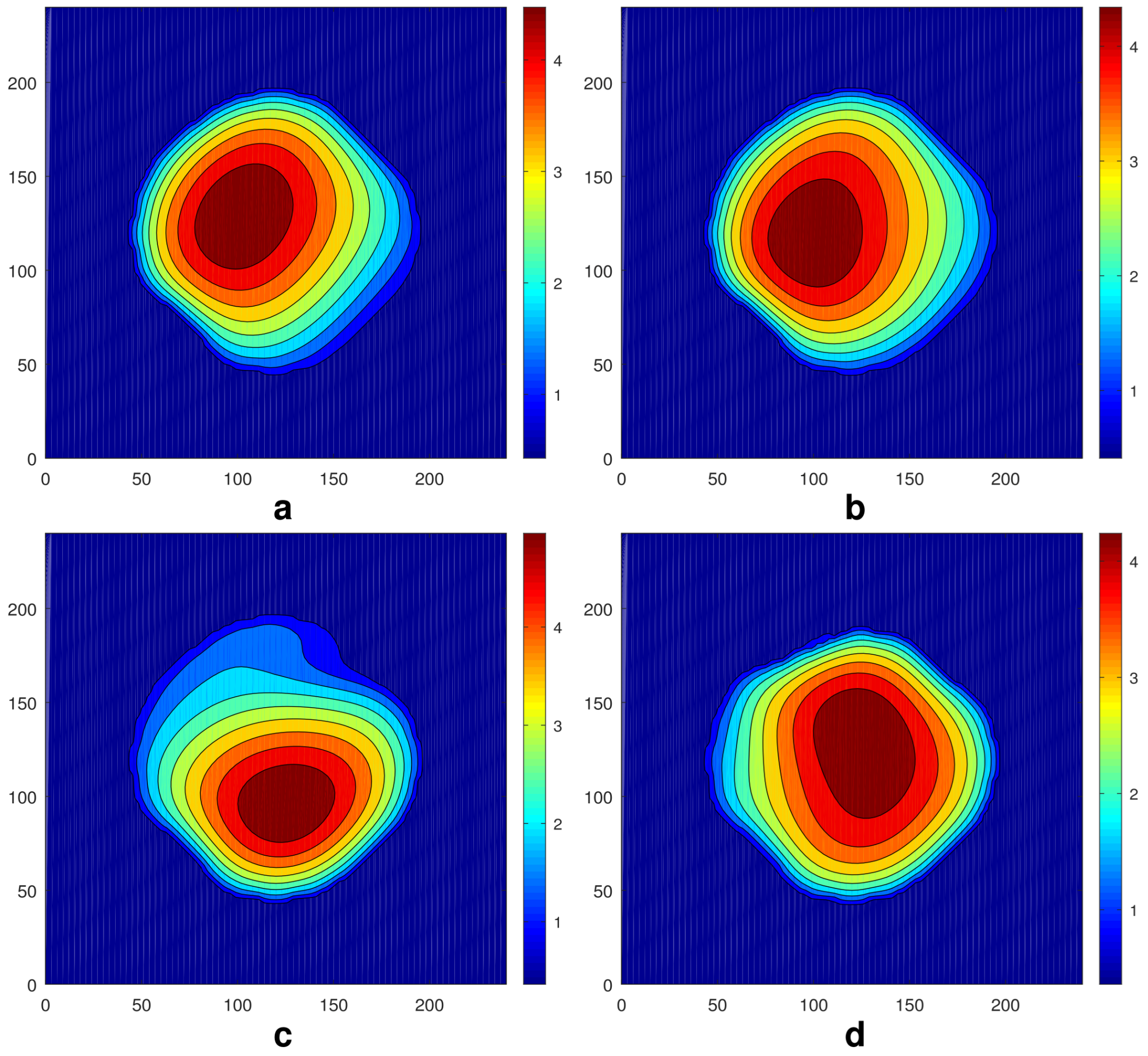
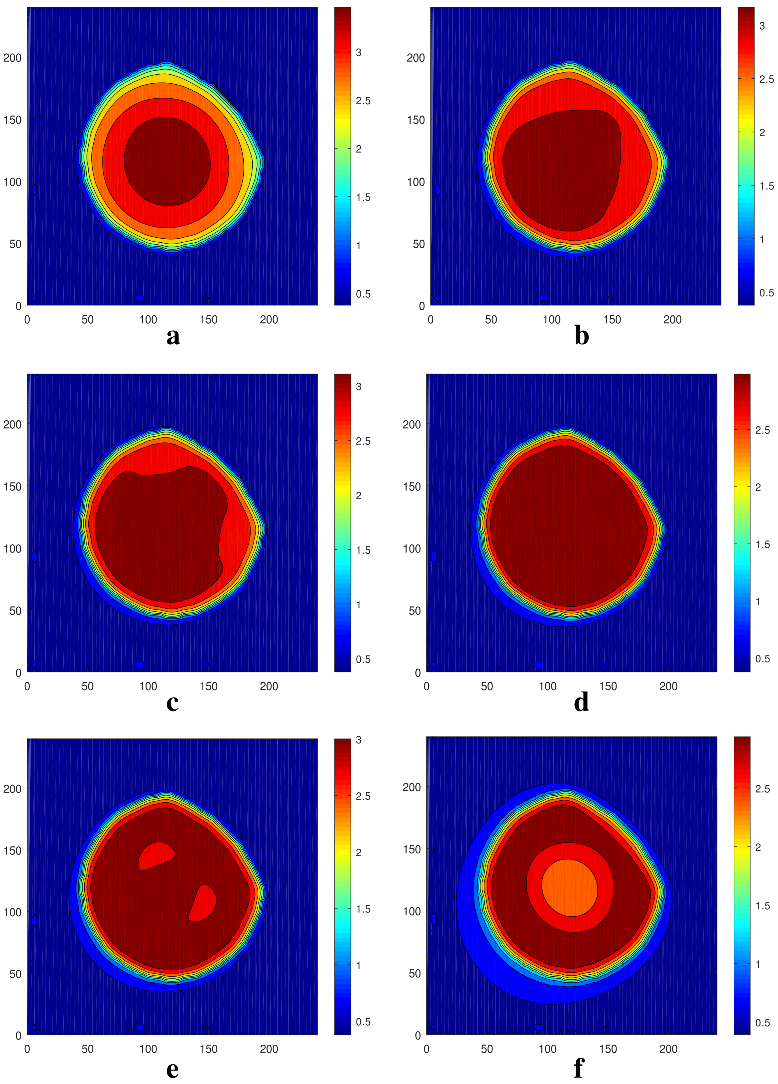
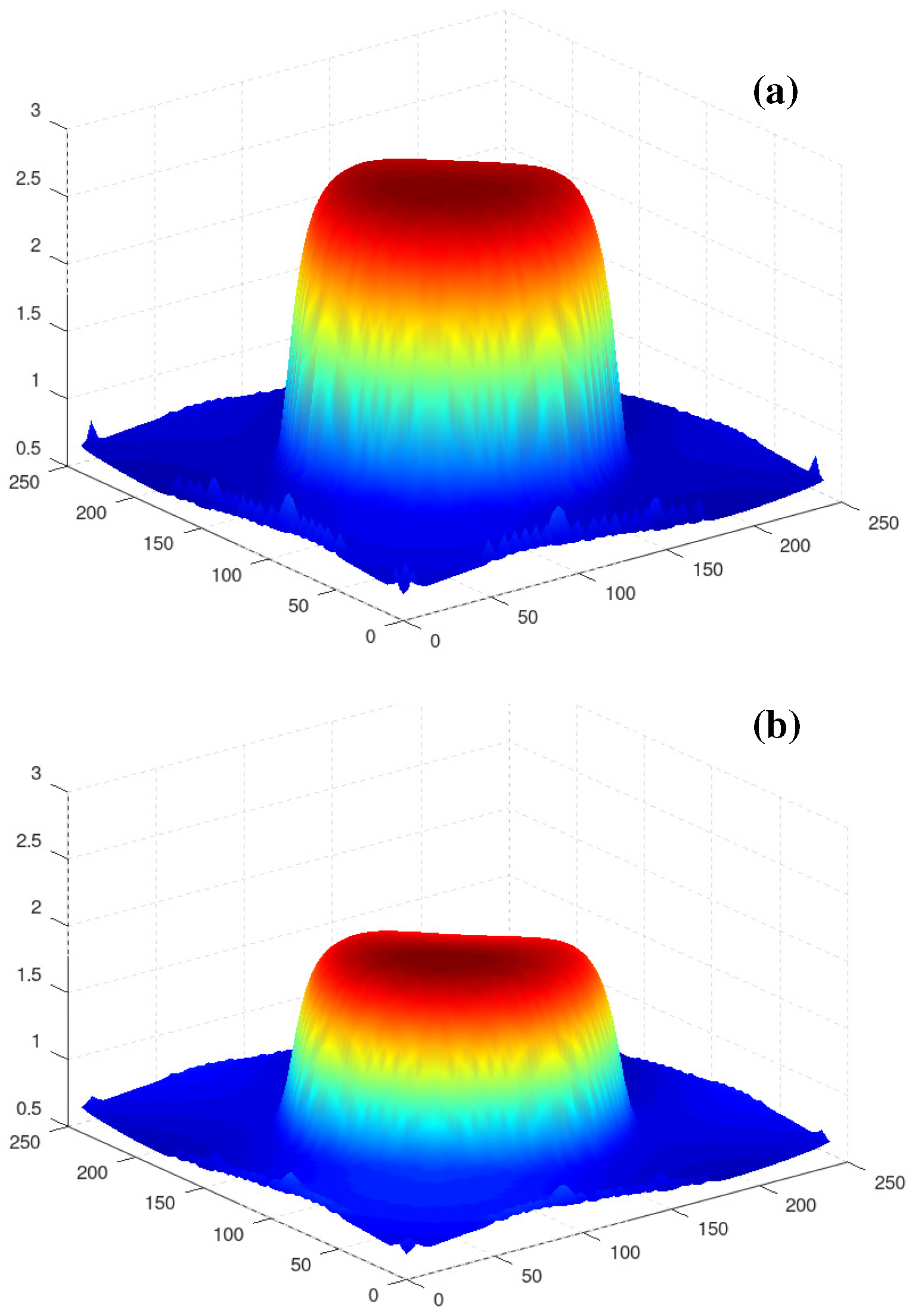
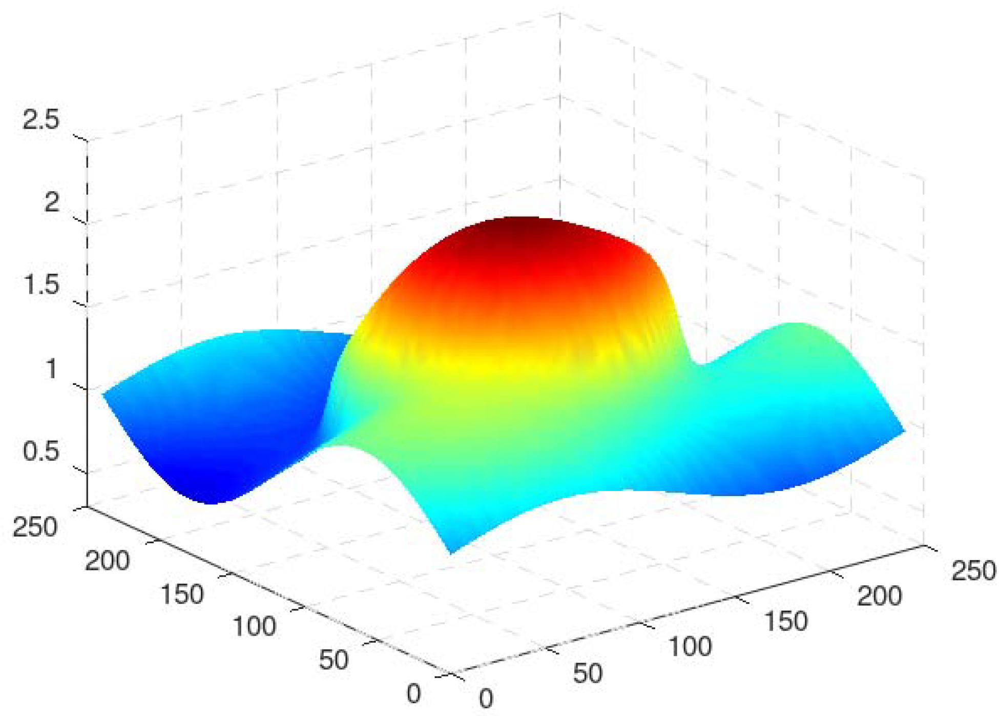
Let us consider now the action of an increased temperature modulation, , on the initially round steady droplet. The intermediate states of the evolution of the initially round droplet under the action of two-dimensional temperature modulation are presented in Figure 4. As in the previous case, in the early stages the liquid in the droplet moves to the left bottom part of the computational region (Figure 4a,b). A visible change in the droplet’s shape takes place between Figure 4a,c. One can see the division of the droplet and the creation of two satellites that are symmetric with respect to the axes (see Figure 4e,f). With an increase in time (at 100,000), the further evolution of the droplet and the equilibration takes place. Finally, we obtain a steady droplet with the maximum significantly shifted along the axis to the region . A snapshot of the fields of (a) and (b) at the equilibrium stage is shown in Figure 5 and the corresponding shapes of interfaces are presented in Figure 6. The droplet keeps the symmetry with respect to the axis . One can see that the droplet becomes much shorter in the direction of the axis (see Figure 5). Let us note that the droplet is significantly higher than that obtained in the case (cf. Figure 3 and Figure 5).
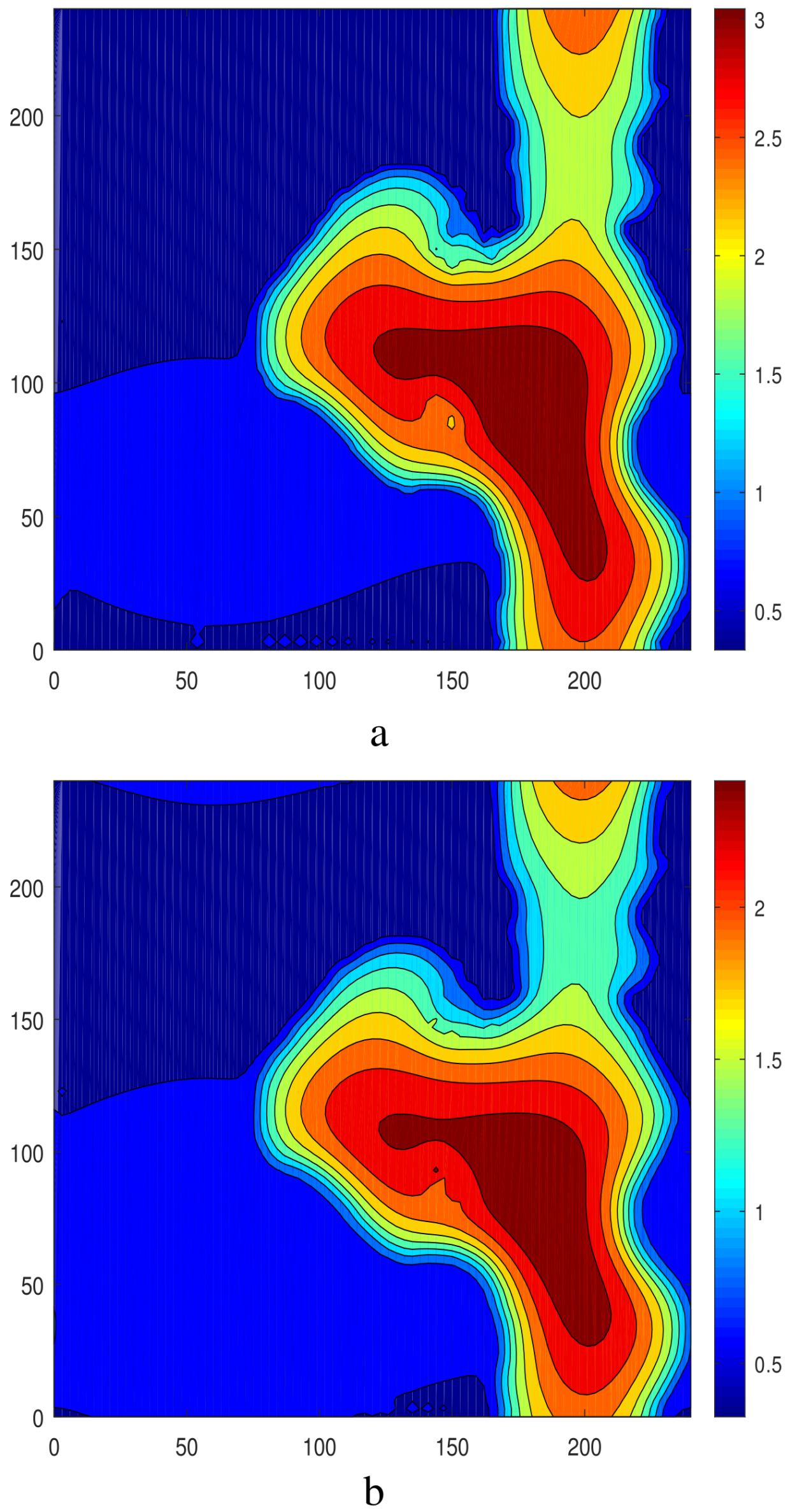
Under the action of the asymmetric field () on the steady round droplet, the symmetry of the initially round droplet is broken. A snapshot of the fields of (a) and (b) is shown in Figure 7, and the shapes of the interfaces are presented in Figure 8. Now, there is no symmetry with respect to the axis (cf. Figure 3 and Figure 7).
3.2. The Case of Nonaxisymmetric Initial Conditions
Let us take now the steady droplet with the maximum, shifted to the left part of the computational region (see Figure 3 in [25]), as the initial conditions and consider its evolution under the action of two-dimensional temperature modulation (; ). Despite the symmetry of the spatial temperature modulation, we obtain an asymmetric steady state. A snapshot of the fields of (a) and (b) is shown in Figure 9, and the shapes of the interfaces are presented in Figure 10.
4. Droplet Oscillations
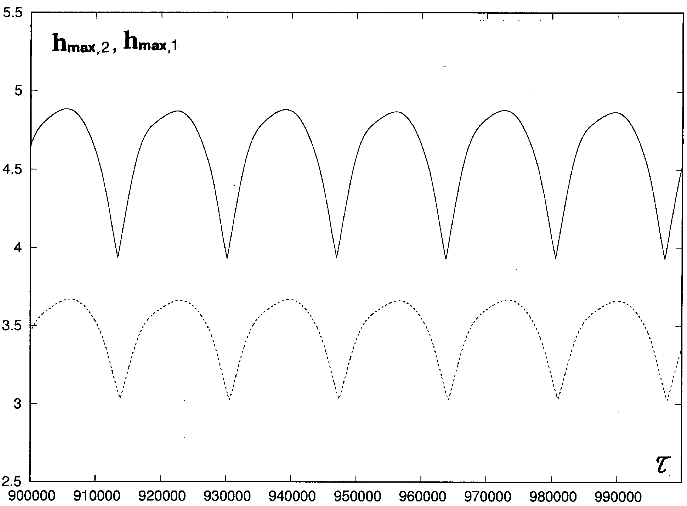
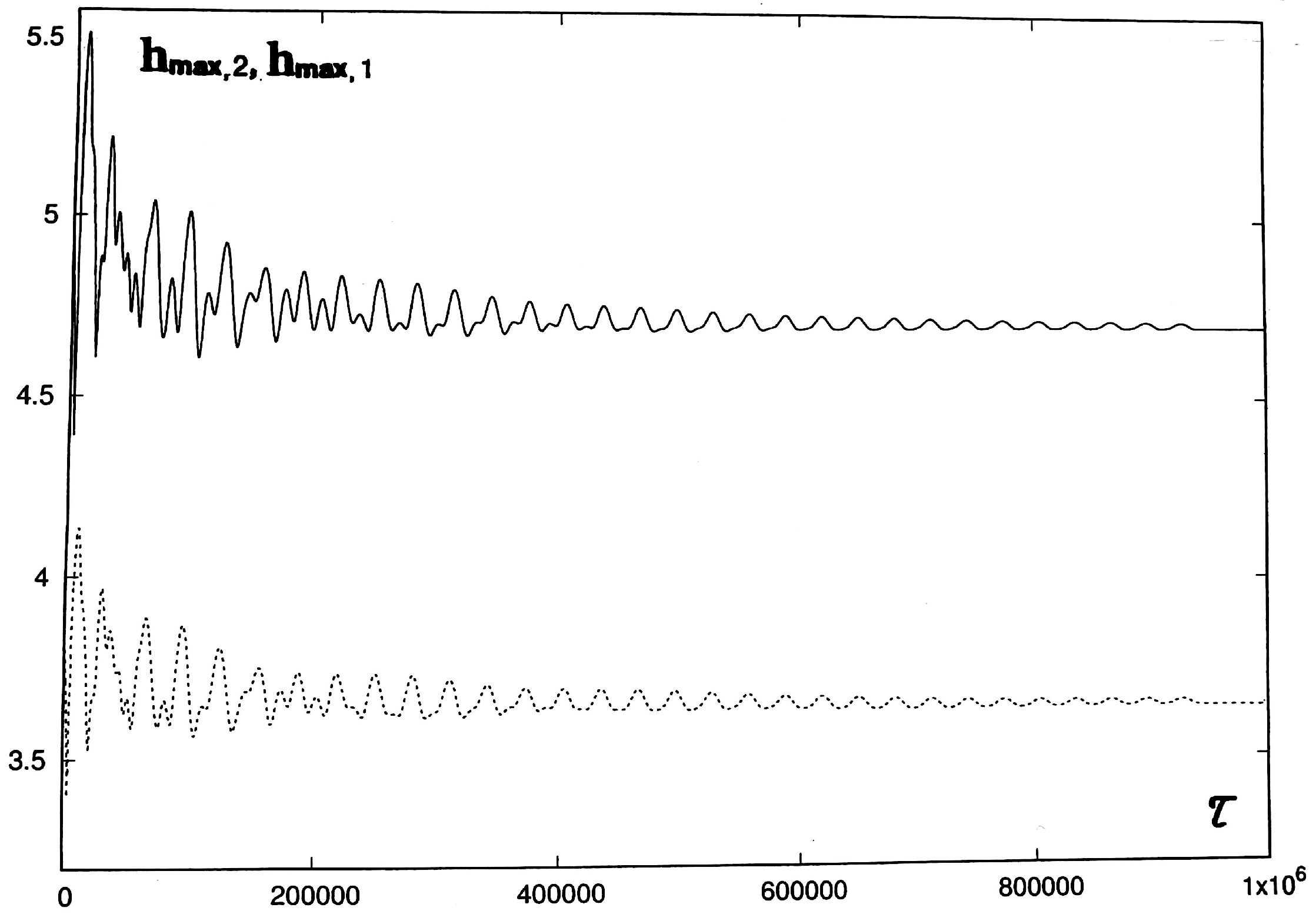
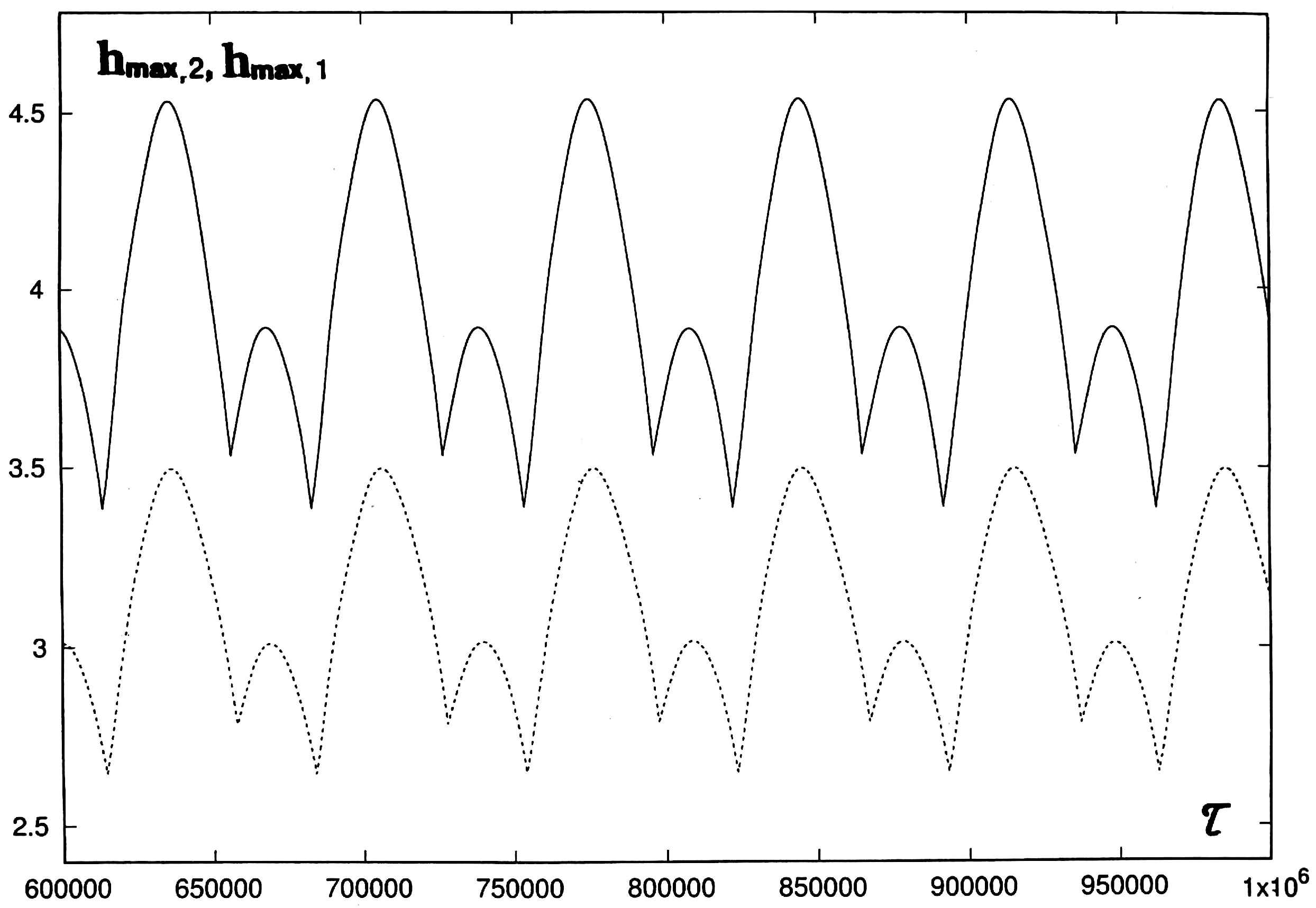
It has been shown in [9] that in the case of a homogeneous cooling from below, the droplet becomes oscillatory unstable with an increase in (see Figure 11). That instability is similar to that formerly found in a system of two flat liquid layers [10]. Let us note that oscillatory Marangoni instabilities for cooling from below have also been observed in some other problems (see [26]).
In the course of oscillations, the droplet keeps the symmetry with respect to the axis . Also, the oscillations are characterized by the symmetry
where T is the period of oscillations. In other words, after the half-period, the shape of the droplet is reflected with respect to the axis . Therefore, the quantities
and
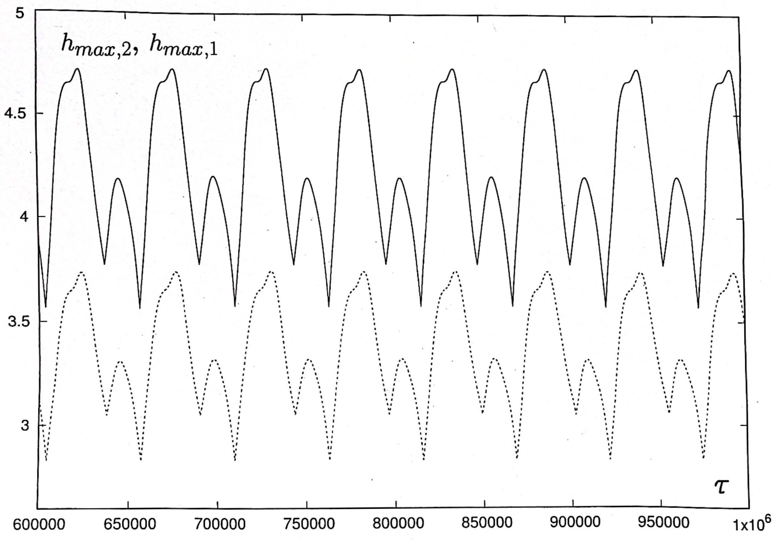
are periodic in time with the period . The temporal evolution of and is shown in Figure 12.
Below, we discuss the influence of the substrate temperature modulation on the oscillatory regime.
4.1. Suppression of Oscillations
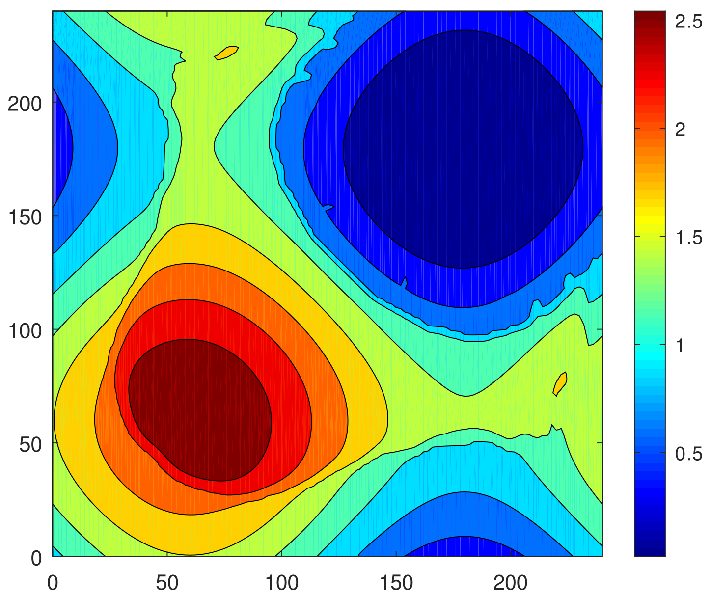
Let us take the oscillatory droplet (see Figure 11 and Figure 12) (; ) as the initial conditions and consider its evolution under the action of two-dimensional spatial temperature modulation (; ). Under the action of the symmetric field , the oscillations are suppressed and the steady state develops in the system. The transient process from the periodic oscillations to the steady droplet is shown in Figure 13, and the intermediate stages of the evolution at different instants of time are presented in Figure 14. One can see that the symmetry of the droplet is broken. Finally, a steady asymmetric droplet is observed in the system. A snapshot of the fields of (a) and (b) at the equilibrium stage is shown in Figure 15, and the corresponding shapes of the interfaces are presented in Figure 16.
Let us consider the influence of asymmetric field on the oscillatory regime presented in Figure 11 and Figure 12—we take and (). In this case, the oscillations are also suppressed and the asymmetric steady droplet develops in the system. A snapshot of the fields of (a) and (b) is presented in Figure 17, and the shapes of the interfaces are shown in Figure 18. The sharp corners in Figure 18 present the connection of the droplet with the neighbor droplet and are created by the crossing of the interfaces with the plane , which cuts the droplet. One can see that the shape of the droplet is rather smooth.
4.2. Excitation of Oscillations
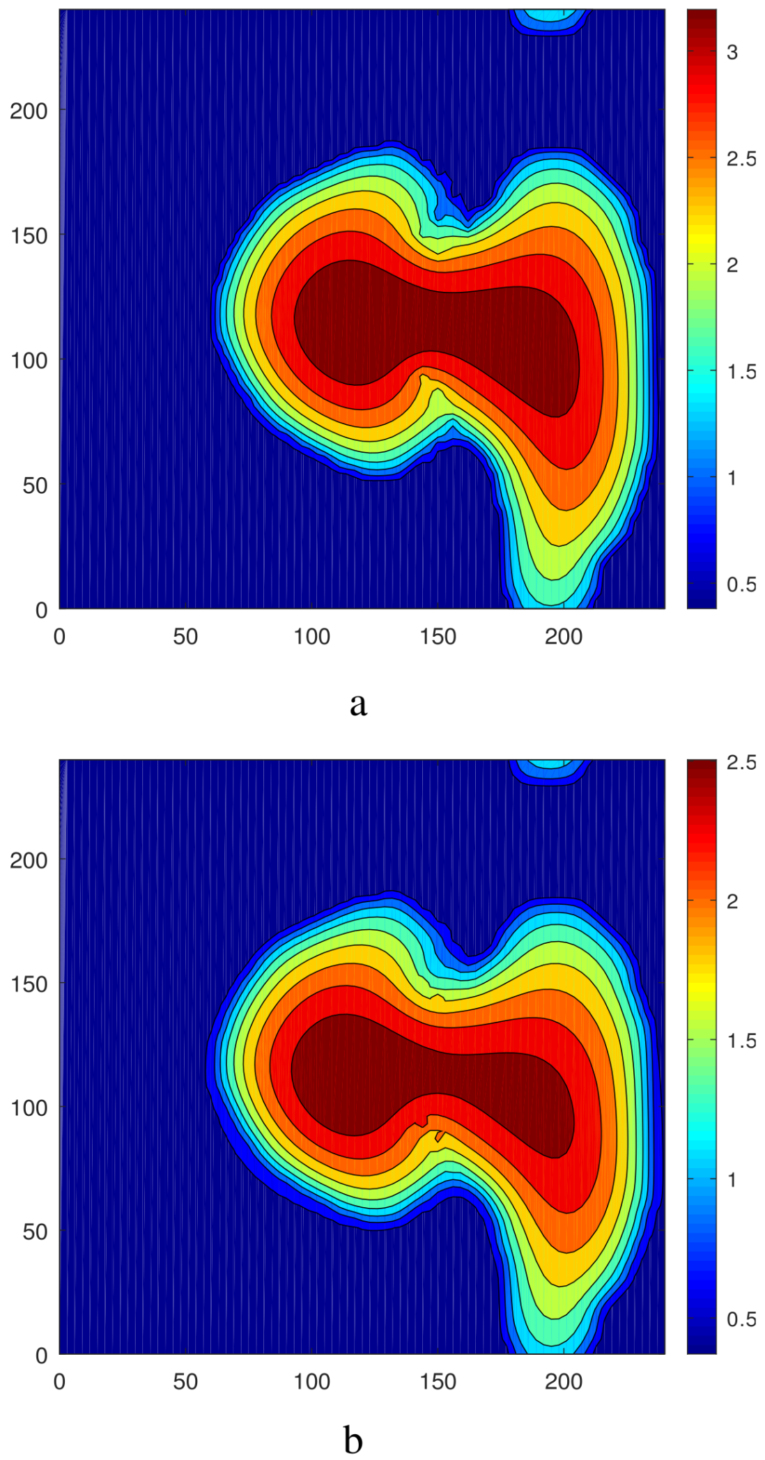
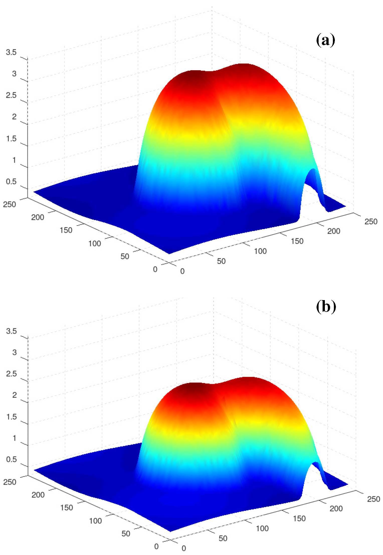
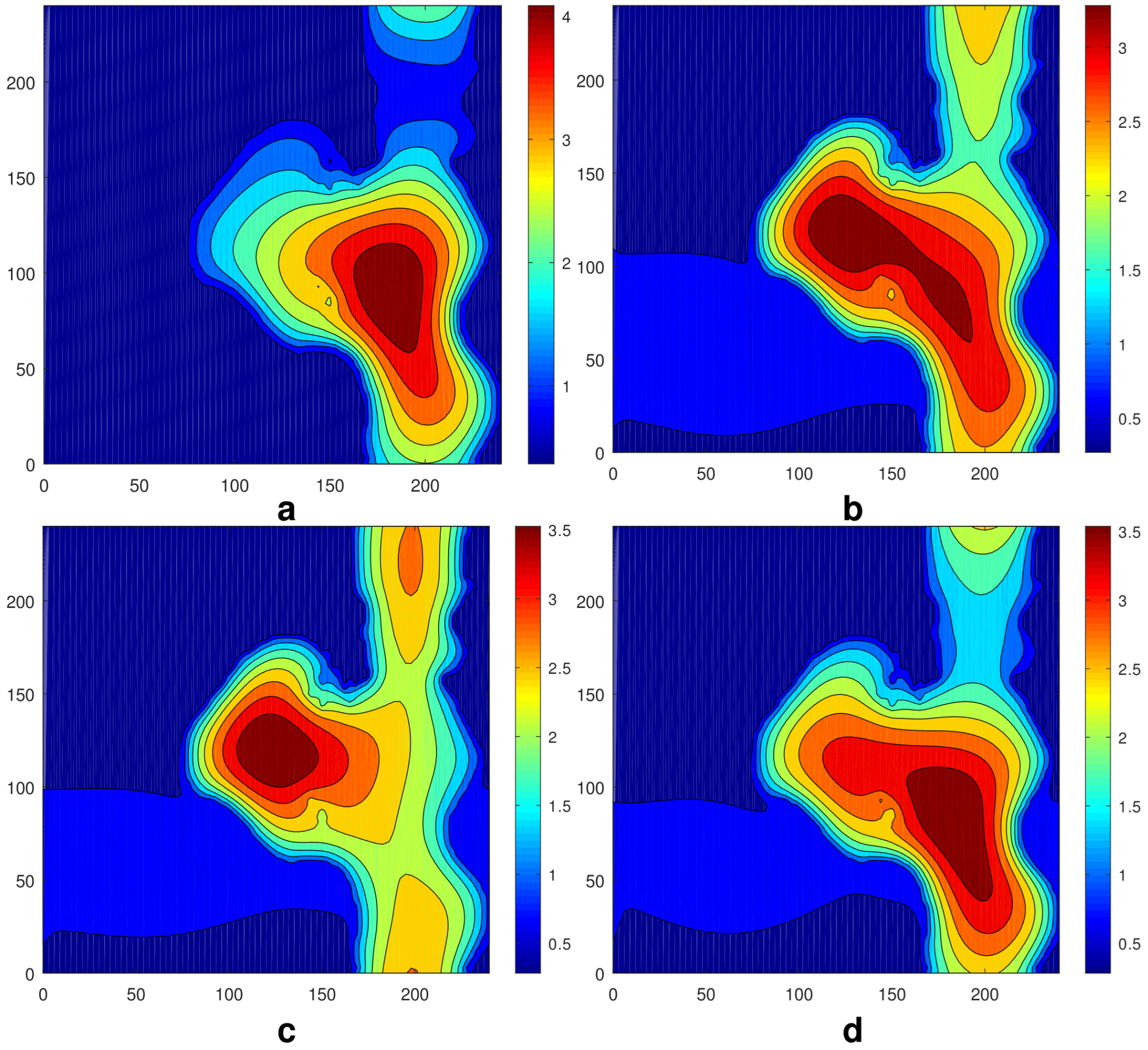
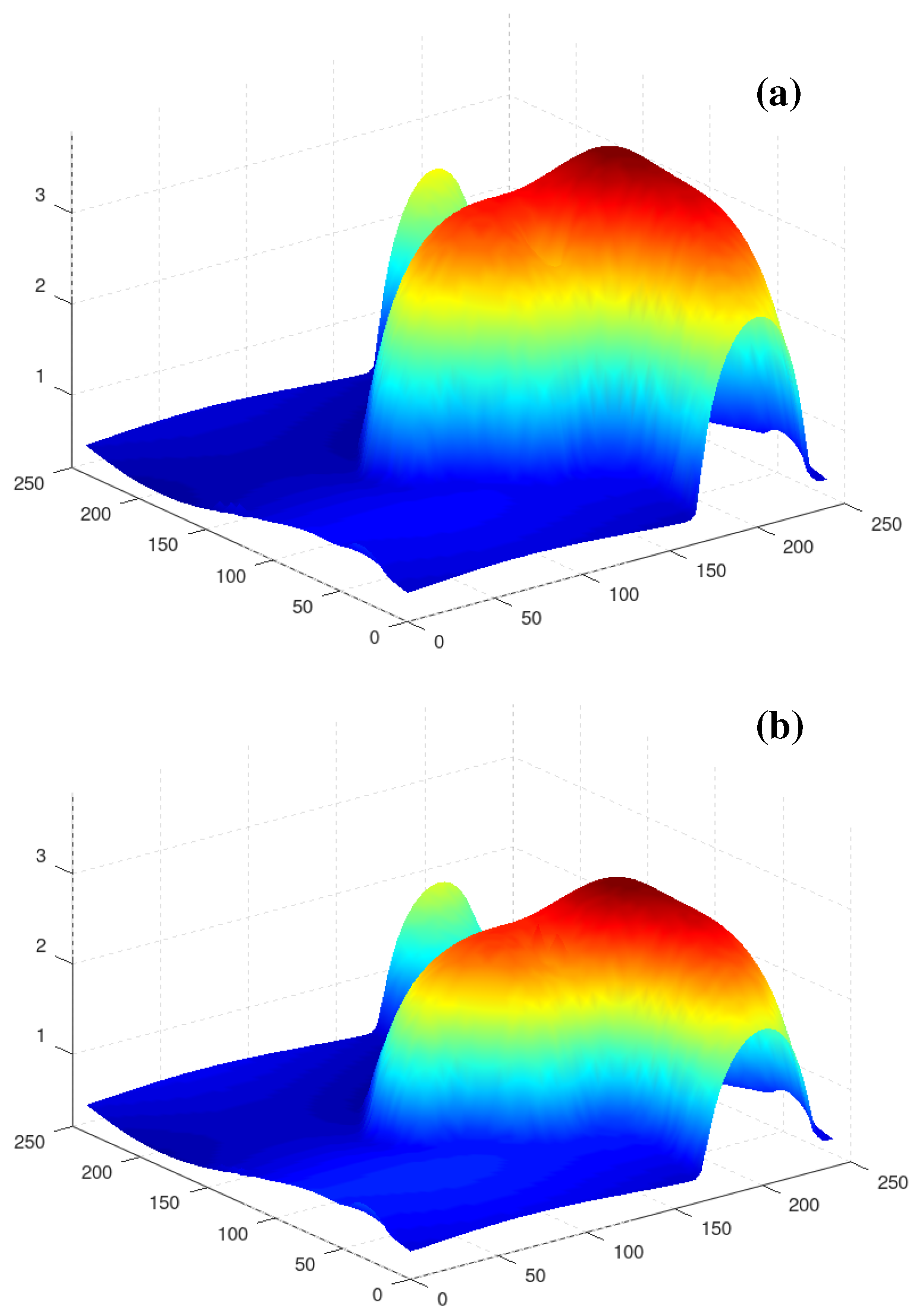
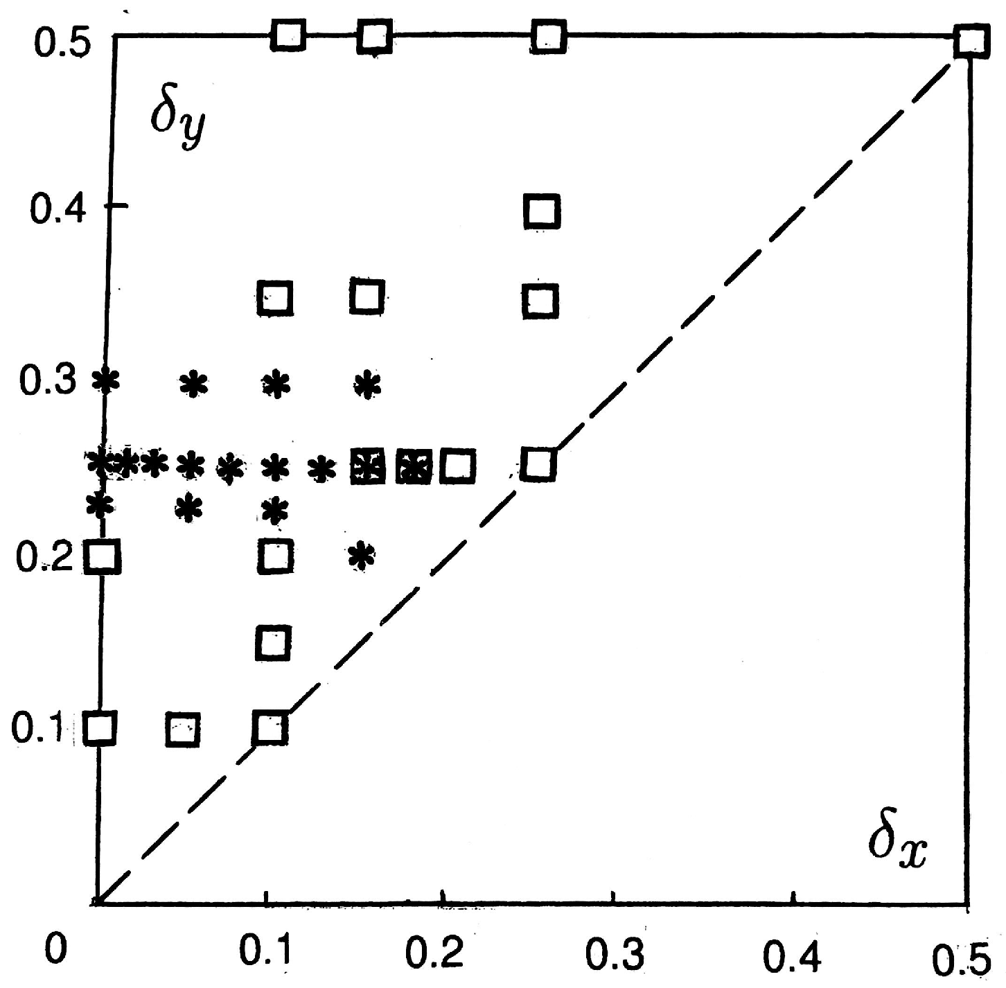
Surprisingly, we observed an excitation of oscillations for , i.e., in the case where in the absence of modulation the round droplet is stable, when we apply an asymmetric field (, ) on the asymmetric steady droplet with the maximum, shifted to the left part of the computational region (see Figure 3 in [25]). In this case, periodic oscillations with essentially different adjacent maxima develop in the system (see Figure 19); the period of oscillations T = 69,420. Snapshots of the fields at different instants of time are presented in Figure 20. The small and big maxima of , , correspond to different spatial points. Let us note that because the different maxima are in the points with different values of , there is no reason for them to be equal. Since we consider the region with periodic boundary conditions, one can see the appearance of a finger that meets the fingers of the neighbor drops at the boundary of the computational region. The combination and the recombination of the droplet with its neighbors could be the origin of the oscillations. The shapes of interfaces, corresponding to Figure 20b, are shown in Figure 21. A diagram of the regimes in the plane (, ) for is presented in Figure 22. One can see that bistability takes place at several points.
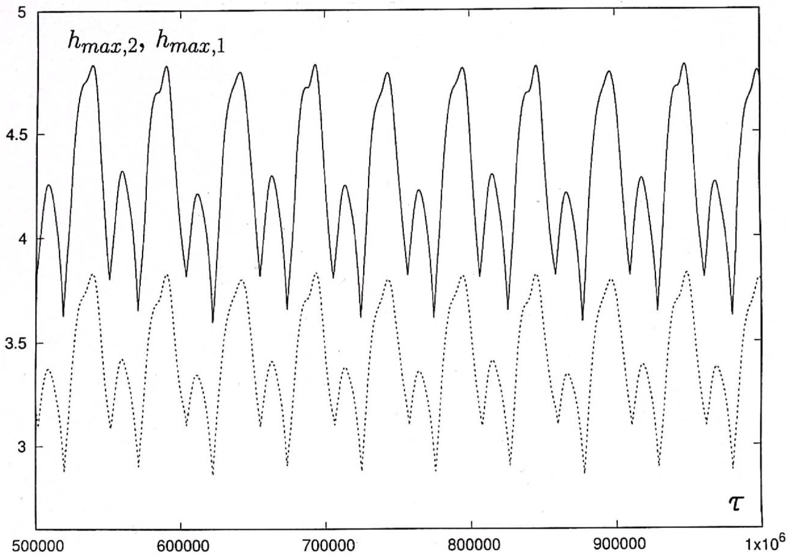
Let us take the oscillatory flow presented in Figure 19 and Figure 20a as the initial condition and consider its evolution at the larger values of . With an increase in , periodic oscillations with different adjacent maxima become of a rather complex form; the amplitude of oscillations grows and the period of oscillations decreases (cf. Figure 23 ( 52,940) and Figure 19 ( 69,420)). At , quasiperiodic oscillations develop in the system (see Figure 24).
5. The Influence of Gravity on the Droplet Dynamics
Now, let us consider the action of gravity on the droplets. If we take the stationary droplet obtained under the action of the symmetric field (, ) as the initial condition (see Figure 3), under the action of gravity (), the droplet is essentially flattened. The intermediate stages of the evolution of the initially round droplet are presented in Figure 25. Under the action of the thermocapillary flow in the substrate directed along the axis , the droplet changes its shape and height. The isolines and the shapes of the interfaces, corresponding to the final equilibrium state, are shown in Figure 26 and Figure 27 (cf. Figure 3 and Figure 26). The droplet still keeps the symmetry with respect to axis .
Under the action of gravity () on the asymmetric stationary droplet shown in Figure 7 (, ; ), we obtain the asymmetric significantly flattened droplet (cf. Figure 7 and Figure 28).
Let us take as initial conditions the periodic oscillations presented in Figure 19 and Figure 20a. Under the action of sufficiently small gravity (), oscillations are suppressed and the steady droplet develops in the system. A snapshot of the fields of (a) and (b) is shown in Figure 29. The height of the droplet is essentially lower than that obtained in the absence of gravity (cf. Figure 20a and Figure 29a).
6. The Influence of the Biot Number on the Shape of the Droplet
Let us consider the influence of the Biot number on the shape of droplets. We take the stationary droplet obtained under the action of the symmetric field (, ) as the initial conditions (see Figure 3). With a decrease in , under the action of the thermocapillary flow in the substrate directed along the axis , the droplet is completely destroyed, and we obtain a square pattern. A snapshot of the field , corresponding to the final equilibrium state for a sufficiently small value of , is shown in Figure 30. The pattern keeps the symmetry with respect to axis . The shape of the upper interface is presented in Figure 31. The similar patterns generated by the bottom temperature modulation have been obtained in two-layer films [27].
Let us note that the same steady regime has been obtained from the other initial conditions when a droplet of liquid 2 with a Gaussian shape was imposed on a flat layer of liquid 1.
The redistribution of the liquids in the droplet and in the substrate along the axis with the maximum shifted to the region also takes place for sufficiently small values of (, , ). The intermediate stages of the evolution of the field at different instants of time are presented in Figure 32. A snapshot of the field and the corresponding shape of the upper interface at the final equilibrium state are shown in Figure 33 and Figure 34.
Now, let us take as initial conditions the periodic oscillations presented in Figure 19 and Figure 20a. With a decrease in (at ), oscillations are suppressed and the steady asymmetric droplet develops in the system. A snapshot of the field of is shown in Figure 34. Let us note that the asymmetric droplet has also been obtained for sufficiently small values of and (, ). The isolines and the shape of the upper interface, corresponding to the final equilibrium state, are shown in Figure 35 and Figure 36. One can see that the symmetry with respect to axis is broken.
7. Conclusions
The dynamics of a droplet on a liquid substrate in the case of an inhomogeneous cooling from below has been investigated. The problem is studied numerically in the framework of the longwave approximation and the precursor model.
It is shown that a two-dimensional spatial inhomogeneity of the substrate temperature creates more diverse flow regimes than a one-dimensional temperature inhomogeneity.
The nonhomogeneous cooling creates a disbalance of thermocapillary stresses that leads to the redistribution of the liquids in the droplet and in the substrate. It is found that the droplet can be stationary or subject to oscillations caused by an oscillatory Marangoni instability. The two-dimensional spatial inhomogeneity of the temperature enhances the oscillatory instability threshold, and it can suppress oscillations, leading to the formation of steady droplets. In a definite region of parameters, the two-dimensional spatial modulation can lead to the excitation of the specific type of periodic oscillations with different adjacent maxima. A diagram of regimes in the plane (, ) has been constructed. The bistability in several points has been obtained. The gravity flattens the droplet and suppresses oscillations.
The influence of the Biot number on the shape of the droplet has been studied. The smaller the , the stronger the inhomogeneities of the temperature on the free surface and, thus, the stronger the action of the thermocapillary effect. Square patterns similar to those generated by the bottom temperature modulation in two-layer films have been obtained.
Author Contributions
A.N. and I.S. wrote the paper together. All authors have read and agreed to the published version of the manuscript.
Funding
This research was supported by the Israel Science Foundation (grant No. 843/18).
Data Availability Statement
Data are contained within the article.
Conflicts of Interest
The authors declare no conflict of interest.
References
- de Gennes, P.G. Wetting: Statics and dynamics. Rev. Mod. Phys. 1985, 57, 827. [Google Scholar] [CrossRef]
- de Gennes, P.G.; Brochard-Wyart, F.; Quérxex, D. Capillarity and Wetting Phenomena: Drops, Bubbles, Pearls, Waves; Springer: Berlin/Heidelberg, Germany, 2004. [Google Scholar]
- Labanieh, L.; Nguyen, T.N.; Zhao, W.A.; Kang, D.K. Floating droplet array: An ultrahigh-throughput device for droplet trapping, real time analysis and recovery. Micromachines 2015, 60, 1469–1482. [Google Scholar] [CrossRef] [PubMed]
- Yamini, Y.; Rezazadeh, M.; Seidi, S. Liquid-phase microextraction—The different principles and configurations. TRAC—Trends Anal. Chem. 2019, 112, 264–272. [Google Scholar] [CrossRef]
- Ju, G.; Yang, X.; Li, L.; Cheng, M.; Shi, F. Removal of oil spills through a self-propelled smart device. Chem. Asian J. 2019, 14, 2435–2439. [Google Scholar] [CrossRef] [PubMed]
- Rybalko, S.; Magome, N.; Yoshikawa, K. Forward and backward laser-guided motion of an oil droplet. Phys. Rev. E 2004, 70, 046301. [Google Scholar] [CrossRef] [PubMed]
- Song, C.; Moon, J.K.; Lee, K.; Kim, K.; Pak, H.K. Breathing, crawling, budding, and splitting of a liquid droplet under laser heating. Soft Matter 2014, 10, 2679–2684. [Google Scholar] [CrossRef] [PubMed]
- Buffone, C. Formation, stability and hydrothermal waves in evaporating liquid lenses. Soft Matter 2019, 15, 1970–1978. [Google Scholar] [CrossRef]
- Nepomnyashchy, A.; Simanovskii, I. Droplets on the liquid substrate: Thermocapillary oscillatory instability. Phys. Rev. Fluids 2021, 6, 034001. [Google Scholar] [CrossRef]
- Nepomnyashchy, A.A.; Simanovskii, I.B. Marangoni instability in ultrathin two-layer films. Phys. Fluids 2007, 19, 122103. [Google Scholar] [CrossRef]
- Greco, E.F.; Grigoriev, R.O. Thermocapillary migration of interfacial droplets. Phys. Fluids 2009, 21, 042105. [Google Scholar] [CrossRef]
- Yakshi-Tafti, E.; Cho, H.J.; Kumar, R. Droplet actuation on a liquid layer due to thermocapillary motion: Shape effect. Appl. Phys. Lett. 2010, 96, 264101. [Google Scholar] [CrossRef]
- Keiser, L.; Bense, H.; Colinet, P.; Bico, J.; Reyssat, E. Marangoni bursting: Evaporation induced emulsification of binary mixtures on a liquid layer. Phys. Rev. Lett. 2017, 118, 074504. [Google Scholar] [CrossRef]
- Neumann, F. Vorlesungen über die Theorie der Capllarität; Teubner: Leipzig, Germany, 1894. [Google Scholar]
- Kriegsmann, J.J.; Miksis, M.J. Steady motion of a drop along a liquid interface. SIAM J. Appl. Math. 2003, 64, 18. [Google Scholar] [CrossRef]
- Craster, R.V.; Matar, O.K. On the dynamics of liquid lenses. J. Colloid Interface Sci. 2006, 303, 503–516. [Google Scholar] [CrossRef] [PubMed]
- Pototsky, A.; Bestehorn, M.; Merkt, D.; Thiele, U. Morphology changes in the evolution of liquid two-layer films. J. Chem. Phys. 2005, 122, 224711. [Google Scholar] [CrossRef] [PubMed]
- Nepomnyashchy, A.A.; Simanovskii, I.B. Effect of gravity on the dynamics of non-isothermic ultra-thin two-layer films. J. Fluid Mech. 2010, 661, 1–31. [Google Scholar] [CrossRef]
- Nepomnyashchy, A.; Simanovskii, I. Nonlinear Marangoni waves in a two-layer film in the presence of gravity. Phys. Fluids 2012, 24, 032101. [Google Scholar] [CrossRef]
- Oron, A.; Davis, S.H.; Bankoff, S.G. Long-scale evolution of thin liquid films. Rev. Mod. Phys. 1997, 69, 931. [Google Scholar] [CrossRef]
- Pototsky, A.; Oron, A.; Bestehorn, M. Vibration-induced flotation of a heavy liquid drop on a lighter liquid film. Phys. Fluids 2019, 31, 087101. [Google Scholar] [CrossRef]
- Sternling, C.V.; Scriven, L.E. On cellular convection driven by surface tension gradients: Effects of mean surface tension and surface viscosity. J. Fluid Mech. 1964, 19, 321–340. [Google Scholar]
- Géoris, P.; Hennenberg, M.; Lebon, G.; Legros, J.C. Investigation of thermocapillary convection in a three-liquid-layer systems. J. Fluid Mech. 1999, 389, 209–228. [Google Scholar] [CrossRef]
- Princen, H.M. Shape of Interfaces, Drops, and Bubbles. In Surface and Colloid Science; Matijevic, E., Ed.; Wiley: New York, NY, USA, 1969; Volume 2, p. 1. [Google Scholar]
- Nepomnyashchy, A.; Simanovskii, I. Marangoni instabilities of droplets on the liquid substrate under the action of a spatial temperature modulation. J. Fluid Mech. 2022, 936, A26. [Google Scholar] [CrossRef]
- Nepomnyashchy, A.; Simanovskii, I.; Legros, J.C. Interfacial Convection in Multilayer Systems, 2nd ed.; Springer: New York, NY, USA, 2012. [Google Scholar]
- Nepomnyashchy, A.; Simanovskii, I. The influence of two-dimensional temperature modulation on nonlinear Marangoni waves in two-layer films. J. Fluid Mech. 2018, 846, 944–965. [Google Scholar] [CrossRef]
Figure 1.
Geometric configuration of the region and coordinate axes.

Figure 2.
The fields of for , , and : (a) ; (b) ; (c) ; (d) = 10,000.

Figure 3.
A snapshot of the fields of and for , , , and .

Figure 4.
The fields of for , , and : (a) ; (b) ; (c) ; (d) ; (e) (f) .

Figure 5.
A snapshot of the fields of and for , , , and .

Figure 6.
The shapes of (a) and (b) for , , , and .

Figure 7.
A snapshot of the fields of and for , , , and .

Figure 8.
The shapes of (a) and (b) for , , , and .

Figure 9.
A snapshot of the fields of (a) and (b) for , , , and .

Figure 10.
The shapes of (a) and (b) for , , , and .

Figure 11.
A snapshot of the fields of for , and : (a) ; (b) .

Figure 12.
The oscillations of (solid line) and (dashed line) for and .

Figure 13.
The oscillations of (solid line) and (dashed line) for , , and .

Figure 14.
The fields of for , , and : (a) ; (b) ; (c) = 10,000; (d) = 20,000.

Figure 15.
A snapshot of the fields of (a) and (b) for , , , and .

Figure 16.
The shapes of (a) and (b) for , , , and .

Figure 17.
A snapshot of the fields of (a) and (b) for , , , , and .

Figure 18.
The shapes of (a) and (b) for , , , and .

Figure 19.
The oscillations of (solid line) and (dashed line) for , , , and .

Figure 20.
The fields of for , , and : (a) ; (b) ; (c) ; (d) .

Figure 21.
The shapes of (a) and (b) for , , , , and .

Figure 22.
Diagram of regimes on the plane for , and : empty square, stationary pattern; asterisk, oscillatory flow.
Figure 22.
Diagram of regimes on the plane for , and : empty square, stationary pattern; asterisk, oscillatory flow.

Figure 23.
The oscillations of (solid line) and (dashed line) for , , , and .

Figure 24.
The oscillations of (solid line) and (dashed line) for , , , and .

Figure 25.
The fields of for , , and : (a) ; (b) ; (c) ; (d) ; (e) (f) .

Figure 26.
A snapshot of the fields of and for , , , and .

Figure 27.
The shapes of (a) and (b) for , , , and .

Figure 28.
A snapshot of the fields of and for , , , and .

Figure 29.
A snapshot of the fields of and for , , , and .

Figure 30.
A snapshot of the field of for , , , and .

Figure 31.
The shape of the interface for , , , and .

Figure 32.
The fields of for , , and : (a) 10,000: (b) 25,000; (c) 40,000; (d) 80,000.

Figure 33.
A snapshot of the field of for , , , and .

Figure 34.
The shape of the interface for , , , and .

Figure 35.
A snapshot of the field of for , , , and .

Figure 36.
The shape of the interface for , , , and .

Disclaimer/Publisher’s Note: The statements, opinions and data contained in all publications are solely those of the individual author(s) and contributor(s) and not of MDPI and/or the editor(s). MDPI and/or the editor(s) disclaim responsibility for any injury to people or property resulting from any ideas, methods, instructions or products referred to in the content. |
© 2023 by the authors. Licensee MDPI, Basel, Switzerland. This article is an open access article distributed under the terms and conditions of the Creative Commons Attribution (CC BY) license (https://creativecommons.org/licenses/by/4.0/).
Share and Cite
MDPI and ACS Style
Nepomnyashchy, A.; Simanovskii, I. The Influence of Two-Dimensional Temperature Modulation on Floating Droplet Dynamics. Fluids 2024, 9, 6. https://0-doi-org.brum.beds.ac.uk/10.3390/fluids9010006
AMA Style
Nepomnyashchy A, Simanovskii I. The Influence of Two-Dimensional Temperature Modulation on Floating Droplet Dynamics. Fluids. 2024; 9(1):6. https://0-doi-org.brum.beds.ac.uk/10.3390/fluids9010006
Chicago/Turabian StyleNepomnyashchy, Alexander, and Ilya Simanovskii. 2024. "The Influence of Two-Dimensional Temperature Modulation on Floating Droplet Dynamics" Fluids 9, no. 1: 6. https://0-doi-org.brum.beds.ac.uk/10.3390/fluids9010006