
Multiple Steady States in Laminar Rayleigh–Bénard Convection of Air

Institute of Mechanics, Materials and Civil Engineering, Université Catholique de Louvain, 1348 Louvain-la Neuve, Belgium
*
Author to whom correspondence should be addressed.
†
These authors contributed equally to this work.
Fluids 2024, 9(1), 7; https://0-doi-org.brum.beds.ac.uk/10.3390/fluids9010007
Submission received: 9 November 2023
/
Revised: 18 December 2023
/
Accepted: 23 December 2023
/
Published: 26 December 2023
(This article belongs to the Topic Fluid Mechanics)
Abstract
:In this article, we report on numerical simulations of laminar Rayleigh–Bénard convection of air in cuboids. We provide numerical evidence of the existence of multiple steady states when the aspect ratio of the cuboid is sufficiently large. In our simulations, the Rayleigh number is fixed at . The gas in the cube is initially at rest but subject to random small-amplitude velocity perturbations and an adverse temperature gradient. When the flow domain is a cube, i.e., the aspect ratio is equal to unity, there is only one steady state. This state is characterized by the development of a single convective roll and by a symmetric normalized temperature profile with respect to the mid-height. On the contrary, when the aspect ratio is equal to 2, there are five different steady states. Only one of them exhibits a symmetric temperature profile and flow structure. The other four steady states are characterized by two-roll configurations and asymmetric temperature profiles.
1. Introduction
Rayleigh–Bénard convection (RBC) constitutes a common configuration of convective heat transfer and has been studied extensively over the years. The classical RBC problem involves a fluid between two horizontal solid boundaries which are maintained at uniform but different temperatures. The temperature at the bottom boundary is higher than in the top one and, therefore, convective motions are developed by the interplay between the buoyancy and gravity forces. A review of numerical and experimental studies of turbulent RBC can be found in [1].
RBC is characterized by three dimensionless numbers, the Rayleigh and Prandtl numbers and the aspect ratio, . For cuboids, is the width-to-height ratio, whereas for circular cylinders it is the diameter-to-height ratio. In the past, several authors have studied the influence of the aspect ratio on RBC [2,3,4]. Regarding steady states, Gelfgat [5] numerically studied RBC in rectangular enclosures just above the instability threshold and showed that multiple steady states can be obtained, depending on the perturbation of the initial condition. In the experimental study [6] of laminar RBC of water in cylindrical domains with large aspect ratios, it was reported that five different steady states can develop. Subsequently, the authors of [7] studied experimentally and numerically the RBC of water in a cylindrical domain and constructed a bifurcation diagram of the solution branches in terms of the Rayleigh number and in the range of and . In [8], a more extensive bifurcation diagram was proposed for water in cylindrical geometries with and for the same range of . Also, the authors of [9] considered the 2D laminar RBC of air in a square and proposed a stochastic approach for the final steady state in terms of the initial condition. In the same study, the authors predicted that the most probable steady state arising from a low-wave-number perturbation is a single-roll configuration. Further, the authors of [10] conducted numerical simulations of turbulent RBC in a cylindrical domain (, and ) and predicted that multiple states can also be developed in that turbulent regime. Multiple states in natural convection have also been observed in settings different than the classical RBC. Examples include rectangular cavities with heated vertical walls [11] and natural convection of Bingham fluids [12].
With regard to classical RBC, the vast majority of studies on multiple steady states have focused on cylindrical domains whereas steady-state solutions in cuboids have received much less attention. However, it is well known that the shape of the container plays a significant role in the flow patterns developed in RBC [13].
The objective of this article is to provide numerical evidence of the existence of multiple steady states in laminar Rayleigh–Bénard convection in cuboids with large aspect ratio. In order to compute the various steady states, the initial condition that we consider is that of a fluid at rest in which we superimpose different random small-amplitude perturbations and an adverse temperature gradient. Herein, we present results for domains with two different aspect ratios , namely, (cube) and .
2. Governing Equations
We consider the natural convection of air enclosed in a cuboid. The system of governing equations is the low-Mach-number approximation of the compressible Navier–Stokes–Fourier equations [14,15]. In dimensionless form, this system reads
The various flow variables and thermophysical properties are non-dimensionalized by those of a reference state of the working gas. The reference physical parameters are denoted by the subscript r.
In the above equations, , and T stand, respectively, for the density, velocity vector and temperature of the working fluid. Further, is the adiabatic ratio, and is the first-order term of the low-Mach-number expansion of the pressure which is referred to as the “thermodynamic pressure” [15]. In closed domains of fixed volume V, as in the present study, is evaluated by combining the expression for the (constant) mass of the working medium, , with its equation of state. In our study, air is treated as a perfect gas, . Therefore, in dimensionless form we have that
Also stands for the piezometric pressure [16,17], with p being the sum of the dynamic and bulk-viscous pressures [18]. In (2), y is the spatial coordinate in the vertical direction and opposite to gravity, and is twice the deviatoric part of the strain-rate tensor, , with being the identity matrix. Further, , , and stand, respectively, for the specific heat capacity under constant pressure, dynamic viscosity and thermal conductivity of the gas. The transport coefficients and are assumed to follow a Sutherland-type law. In dimensionless form, the presumed law reads
With regard to the left-hand side of the energy Equation (3), we have used the fact that, for a perfect gas, the specific enthalpy is given by . Moreover, is the thermal expansion coefficient; for a perfect gas, .
The top and bottom walls of the domain are maintained at temperatures and , respectively, with . For non-dimensionalization purposes, the height of the domain, H, is the reference length and is the reference temperature. Then, the reference thermodynamic state is that at and the initial thermodynamic pressure . Also, the free-fall velocity, , serves as the reference velocity, with and the difference between the fixed temperatures at the bottom and top walls, . Then, the free-fall time, , is set as the reference time scale of the problem in hand. The relevant dimensionless groups are the Rayleigh , Prandtl , Reynolds and Richardson numbers,
with being the thermal diffusivity of air at the reference state, the reference kinematic viscosity and g the gravitational acceleration.
The governing system (1)–(3) is integrated numerically via the time-accurate algorithm for low-Mach-number flows [15]. This algorithm is based on a second-order accurate predictor–corrector scheme for integration in time. Further, it involves a projection method for the evaluation of the piezometric pressure . The projection step amounts to taking the divergence of the momentum equation which, in conjunction with the continuity equation, leads to a constant-coefficient Poisson equation for . This Poisson equation is then discretized and solved numerically via a linear-system solver. Discretization of spatial derivatives is performed via second-order centered differences. The algorithm is implemented in a collocated grid arrangement because this arrangement offers ease of implementation and straightforward applicability to curvilinear coordinate systems. In order to avoid the problem of pressure odd–even decoupling that is often encountered in such grids, the algorithm is supplemented with a flux-interpolation technique [15] which is the generalization of the original scheme [19] to variable-density flows.
This algorithm has been implemented in a parallel code in C/C++ and uses the PETSc suite of data structures and routines [20]. Parallelization is performed via a Message Passing Interface (MPI). Also, the Poisson equation for is solved with the PETSc routine of PFMG which is a parallel semicoarsening multigrid solver. Validation tests of the algorithm and comparisons with numerical results and experimental data can be found in [15,21], respectively. In the past, this algorithm has been used in numerical studies of forced [22] and natural [23] convection and in a variety of simulations of reacting flows.
3. Numerical Setup
As mentioned above, the computational domain is a cuboid. Its width is denoted by W and is the same in the horizontal (x and z) directions. Thus, the aspect ratio of the domain is given by . Herein, we present results for two different cases. In case 1, the flow domain is a cube, i.e., . In case 2, the aspect ratio is increased to . In both cases, the height of the domain is set at cm.
All boundaries of the domain are no-slip rigid walls. The side walls are adiabatically isolated whereas the top and bottom walls are maintained at uniform temperatures, K and K, respectively. Accordingly, the bottom–top temperature difference is K, while the reference temperature is K. For air at , the Prandtl number is . With regard to reference values, the free-fall velocity is m/s, the free-fall time is s, and the product between the thermal expansion and temperature difference is . With these values, the Rayleigh number is , which corresponds to the supercritical but laminar regime. It is also worth adding that the total temperature variation is in the order of 5% of the reference temperature . This means that the total variation of the density is also close to 5%, while the total variation of the viscosity is approximately 4%. Such variations are not a priori negligible. Accordingly, for purposes of computational accuracy, we opted to employ the low-Mach-number equations in our numerical study.
In terms of initial conditions, we assume that the gas is at rest and impose a linear temperature profile between and . The initial thermodynamic pressure is 1 bar. Also, as noted above, we apply random perturbations to the initial zero-velocity field. The amplitude of the applied perturbations is quite small, namely, 1% of the free-fall velocity . On the other hand, the initial temperature profile is left unperturbed.
Regarding grid resolution, we have employed a mesh size of cells. The mesh is refined in the near-wall regions and stretched away from the walls following a hyperbolic tangent distribution. The height of the largest computational cell (which is located in the center of the domain) is . This mesh conforms to the resolution criteria [24,25,26] in the bulk and the near-boundary regions for direct numerical simulations of turbulent RBC at . Since this mesh is sufficiently fine to resolve all turbulent scales of RBC at , then we can safely assume that it can also resolve all the flow structures of the cases of laminar convection treated herein, in which . Moreover, we have performed simulations with a coarser grid, consisting of cells, and observed only very minor differences in the numerical results. This is another indication that the mesh of cells is appropriate for the purposes of our study.
Each simulation is first conducted for a time period of 600 , before assuming that a steady state has been reached. This time period is sufficient to wash out all transient effects. Subsequently, each simulation is run for an additional period of 400 . In all cases, it has been confirmed that the flow profiles remained constant during this additional period.
4. Results and Discussion
With regard to notation, the horizontal-area () average of a generic quantity U is denoted by . Also, is the deviation of U from in horizonal planes. Results for the thermal field are shown in terms of the normalized temperature, . In order to compute multiple steady states, we have performed several simulations of the two cases by solving the low-Mach-number Equations (1)–(3) with different random perturbations of the initial condition of the velocity field. In other words, for each simulation, a separate field of random velocity perturbations is generated.
4.1. Case 1: Aspect Ratio
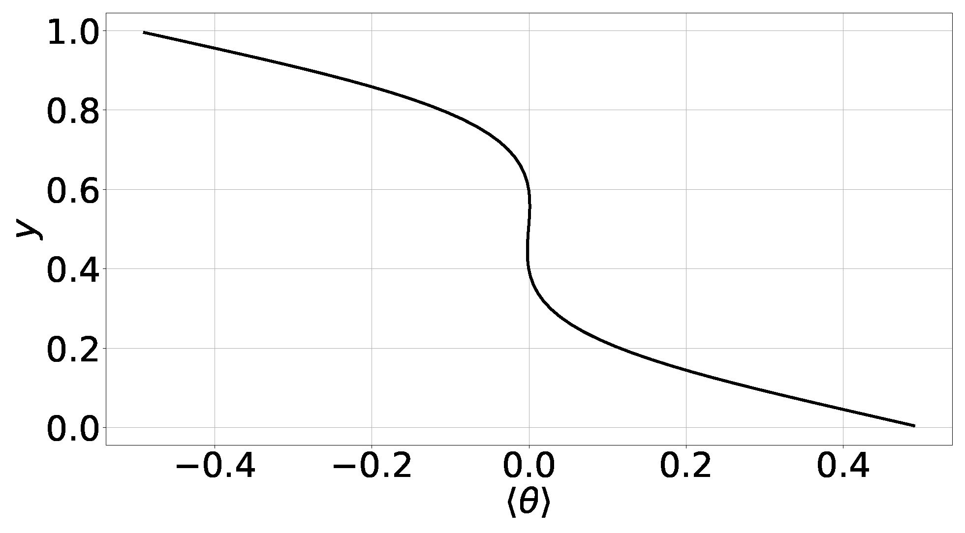
According to our numerical experiments, only one steady state is developed when the aspect ratio is equal to unity. In Figure 1, we have plotted the profile of the area-averaged normalized temperature for this case. We can readily deduce that the profile is practically symmetric with respect to the mid-height. In principle, the profile cannot be completely symmetric due to the variation of the fluid properties (density, viscosity and conductivity) with the temperature. However, as mentioned above, the total (bottom-to-top) variation of the temperature is in the order of 5% and therefore the variations of , and with T are approximately linear. Consequently, the emerging profile of is practically symmetric.
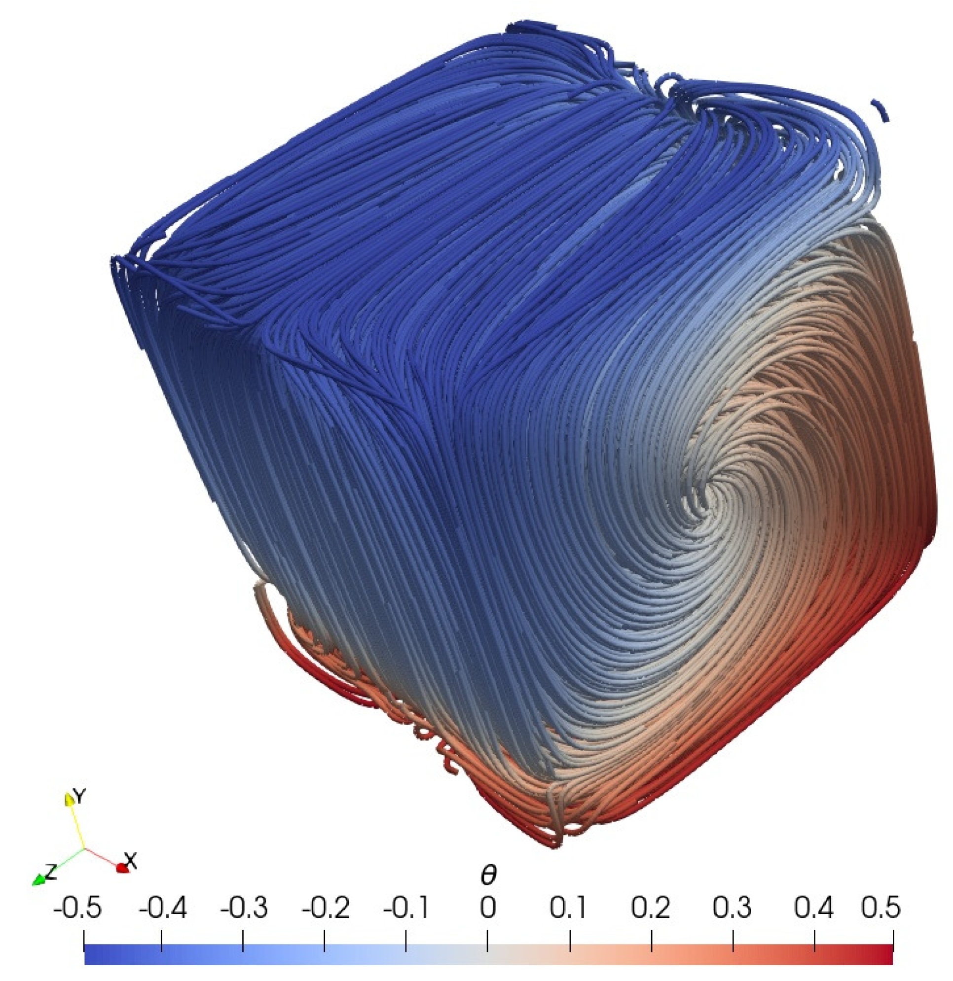
In Figure 2, we present plots of the streamlines colored by for case 1. We observe that the flow is organized into a single large roll which is aligned in one horizontal direction. Also, the streamlines are practically symmetric with respect to the vertical () mid-width plane. As mentioned above, this is due to the small variation of the fluid properties with temperature.
In the context of our study we also performed a simulation of this case by invoking the Boussinesq approximation. According to it, is constant and equal to everywhere in the governing system except for the gravity term in (2) in which . Also, and are constant. Our simulation with the Boussinesq approximation produced nearly identical results for and the streamlines.
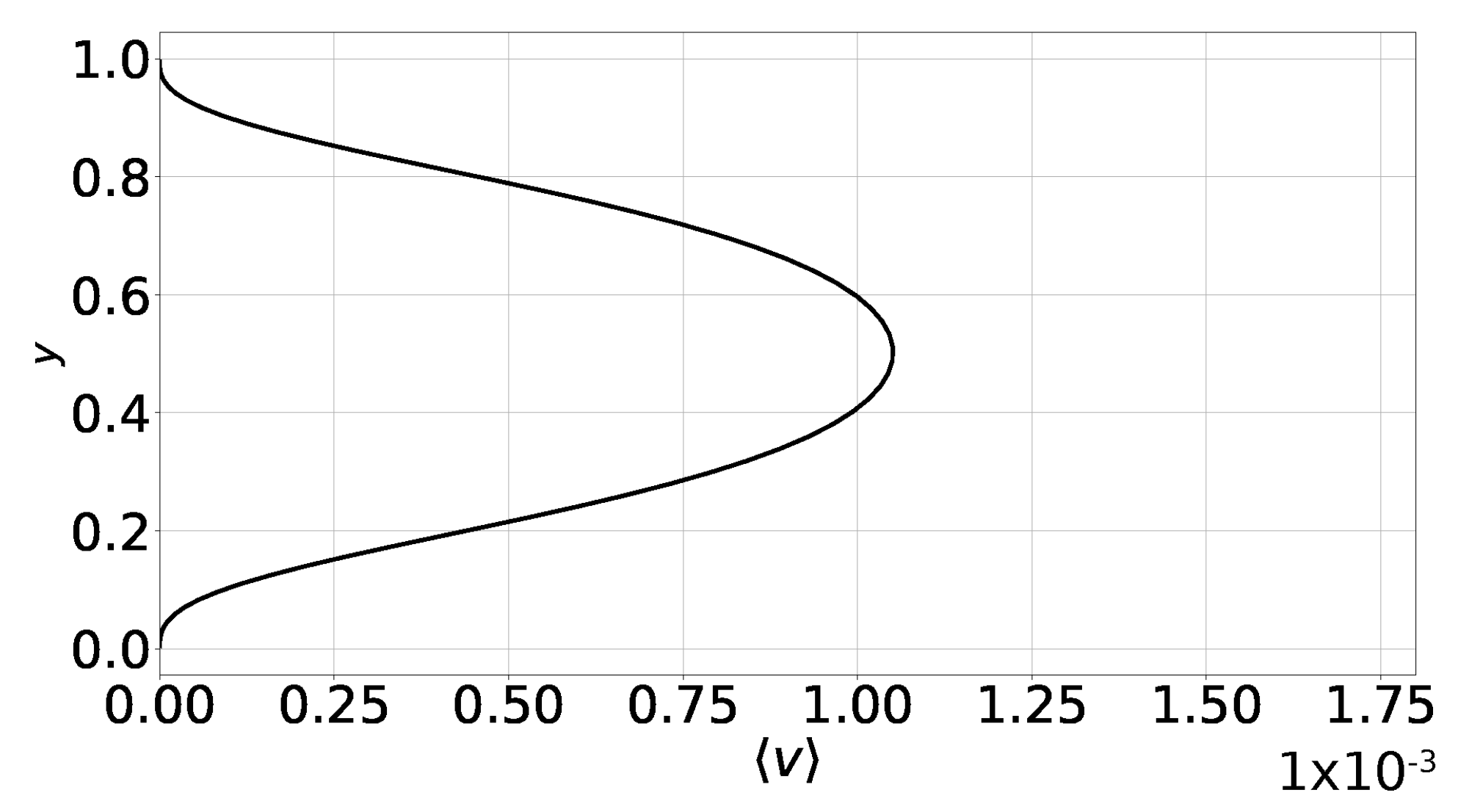
In fact, the only discernible non-Boussinesq effect in our simulation based on the low-Mach-number Equations (1)–(3) is a non-zero mean vertical velocity . Its presence is explained as follows. The mass flux is decomposed according to . For steady flow, ; thus, . In general, is not zero. In Figure 3, we present profiles of for case 1, by solving the low-Mach-number Equations (1)–(3), i.e., without the Boussinesq approximation. According to this figure, the amplitude of is small, albeit non-zero, and peaks at mid-height. On the other hand, under the Boussinesq approximation , hence , are zero.
4.2. Case 2: Aspect Ratio = 2
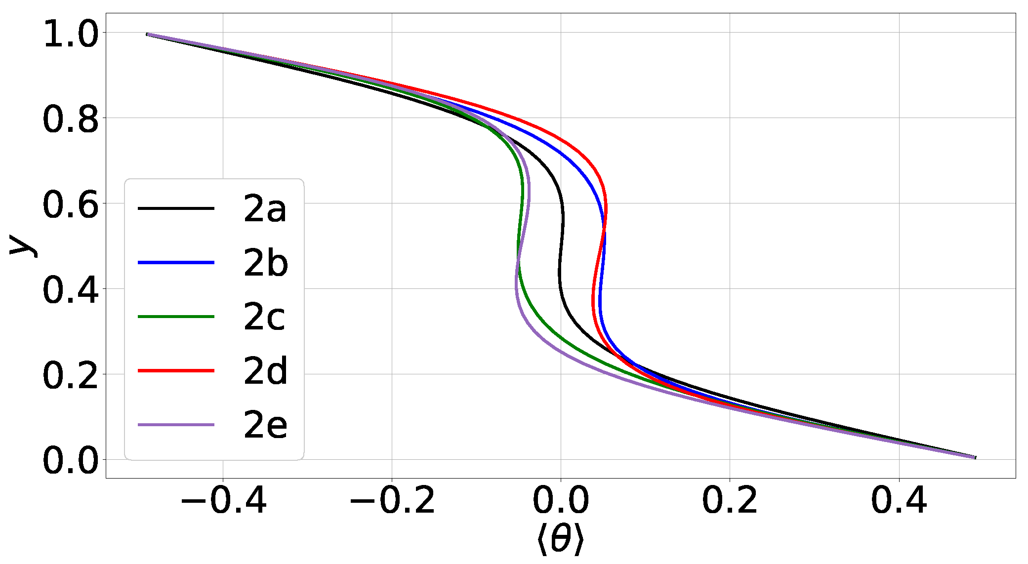
In this section, we examine the case that corresponds to the higher aspect ratio, . By considering different random perturbations on the initial velocity, we were able to compute five different steady states. The profiles of for case 2 are shown in Figure 4. Therein, the various steady solutions are referred to as ‘2a’, ‘2b’ and so on.
In the steady state 2a, the profile of is practically symmetric with respect to the mid-height and close to those in case 1. However, the profiles of the other four steady states are asymmetric and shifted either to the left or to the right, i.e., they are shifted either towards the cold top wall or the warmer bottom one. This asymmetry has been observed in different types of natural convection [11,12] and is associated with the development of more than one convective structure in domains with high aspect ratio. More specifically, this asymmetry is a result of the particular orientation of the flow structures. Our simulations confirm that this is true in classical RBC as well.
We further note that the profiles of are not monotonic but exhibit overshoots at the edges of the thermal boundary layers. Such overshoots have already been predicted in simulations of turbulent RBC [3,27]. In laminar RBC, we attribute these overshoots to the strong ascending and descending plumes which bring substantial amounts of warm gas near the top wall and cold gas near the bottom one, respectively. But since the flow is not turbulent, thermal mixing is not strong enough to reduce the temperature gradients in the bulk of the domain, thereby resulting in such overshoots.
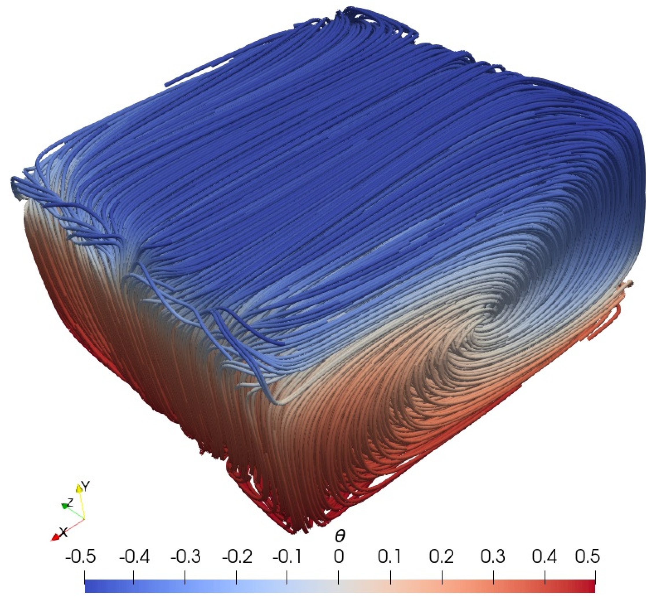
Next, we examine the flow structures in the five different steady states. In Figure 5, we present the streamlines for the steady state 2a, colored by the normalized temperature . The flow is organized into a single large roll which is aligned in one horizontal direction. Further, similarly to the profile, the streamlines are symmetric with respect to the vertical mid-width plane.
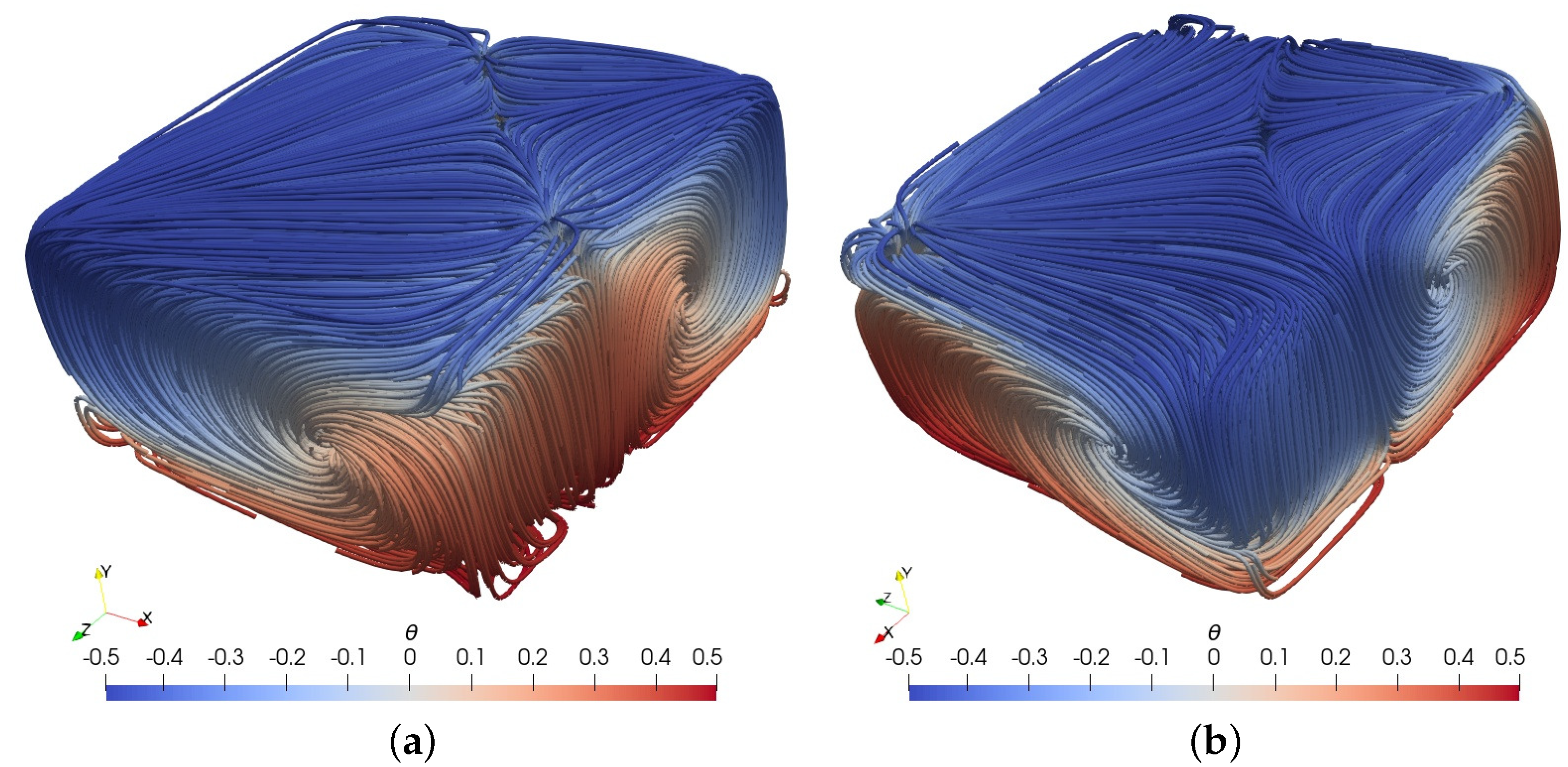
In Figure 6, we have plotted the streamlines of the steady states 2b and 2c. In these states, the flow is organized into two large counter-rotating rolls. These rolls have different sizes but are both aligned in a diagonal plane. The particular diagonal plane of alignment may vary, depending on the perturbation of the initial condition for the velocity. As a result, the streamlines are no longer symmetric with respect to the mid-width plane, which in turn explains the shift of the corresponding profiles. Globally, the flow patterns in 2b and 2c are the same but with opposite direction of rotation of the large rolls.
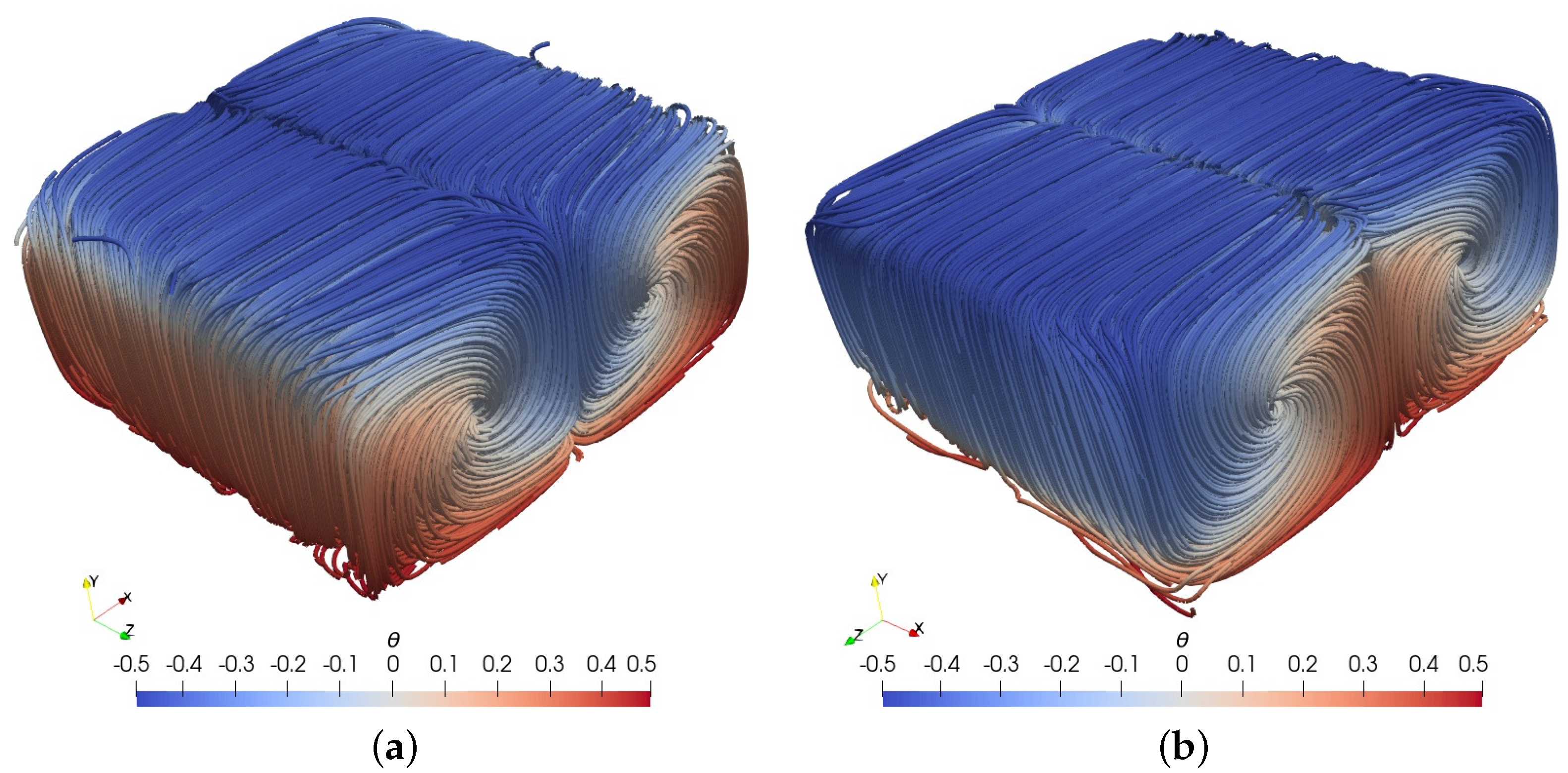
Plots of the streamlines of the steady states 2d and 2e are presented in Figure 7. According to these plots, the flow is organized again into two large counter-rotating rolls. However, these rolls now have equal sizes and are aligned in a horizontal direction, instead of being aligned in a diagonal plane. Further, the flow patterns in 2d and 2e are the same, but with opposite direction of rotation of the large rolls. Upon comparison of the plots in Figure 6 and Figure 7, we infer that in the steady states 2b and 2d, in which the profile is shifted towards the hot bottom wall, the fluid in contact with the side walls is mostly hot whereas in the other two states, 2c and 2e, the profile is shifted towards the top cold wall while the fluid in contact with the side walls is mostly cold.
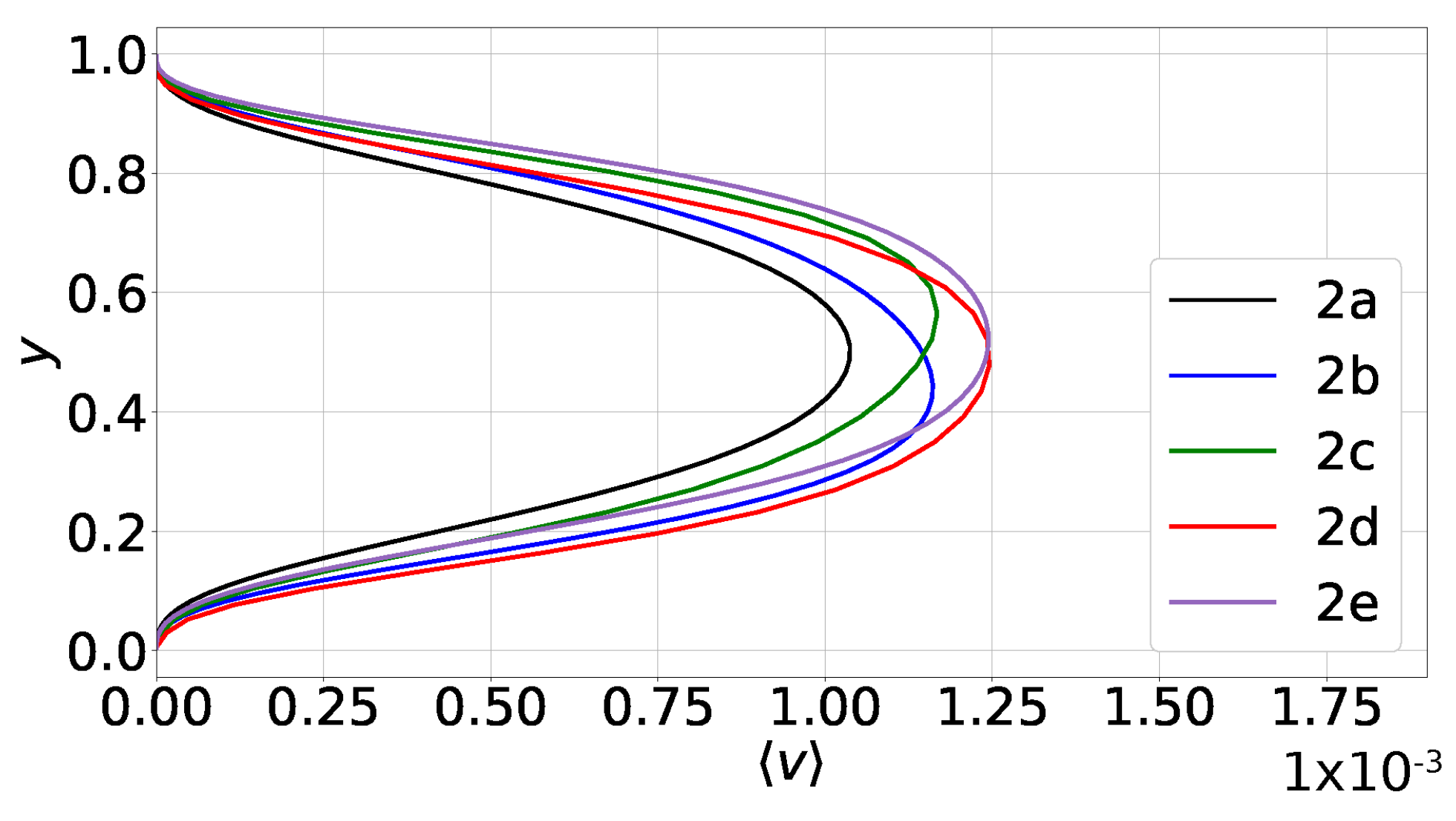
Additional information about the differences between the emerging steady states can be obtained by examining the profiles of the area-averaged horizontal velocity . The plots of for the steady states of case 2 are shown in Figure 8. Globally, these profiles are M-shaped, with a local minimum near the mid-height and two peaks at and , respectively. As with the other flow variables, only the profile of the single-roll state 2a is symmetric. In the other four states, the profiles are asymmetric and the peak values are different. More specifically, in the two-roll states 2b and 2d (whose profile is shifted towards the hot bottom wall), the highest peak is the lower one. As will be shown below, the same is true for the vertical velocity component. This in turn implies that, in 2b and 2d, convective motions and heat transfer are stronger in the lower part of the domain.
On the contrary, in the two-roll states 2c and 2e (whose profile shifted towards the top cold wall), the highest peak of is the upper one. In these states, the vertical velocity also peaks at the top part of the domain. Therefore, in steady states 2c and 2e, convective motions are stronger in the upper part of the domain.
Plots of the mean vertical velocity component, , are presented in Figure 9. According to those, the values of are the highest in states 2d and 2e, i.e., when the flow is organized in two rolls aligned in a horizontal direction. Next, in descending order, are the values of in cases 2b and 2c which are characterized by two rolls aligned in a diagonal plane. Finally, the smallest values are predicted in the single-roll state 2a. As mentioned above, these observations imply that the flow arrangement of cases 2d and 2e exhibits the strongest convective motions.
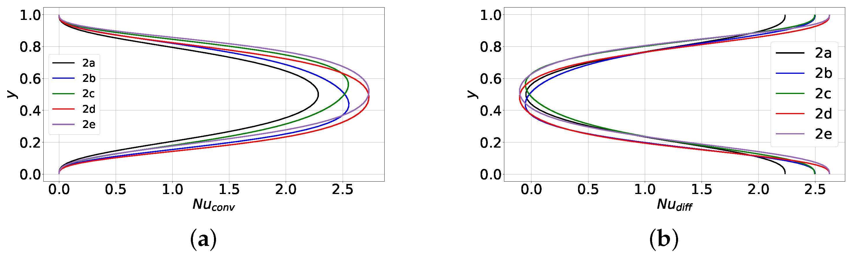
Next, we present results for the Nusselt number. The area-averaged Nusselt number Nu is given by
In the above equation, Nu represents the convective contribution and Nu the diffusive one. At steady state, should be constant and equal to the global Nusselt number. This was indeed predicted by our simulations. The profiles of Nu and Nu are shown in Figure 10a and Figure 10b, respectively. We observe that Nu takes small negative values near the center of the domain. This is due to the fact that the profiles of are not monotonic but instead exhibit two overshoots.
As expected, the profile of Nu in steady state 2a is symmetric whereas in states 2b and 2d the profile is shifted downwards. This further corroborates that in 2b and 2d, convective heat transfer is stronger in the lower part of the domain. The opposite is true for the steady states 2c and 2e, i.e., the Nu profile is shifted upwards because convection is stronger in the upper part of the domain. These findings are in accordance with the predicted velocity profiles. Further, from the plots of Figure 10 we infer that the states 2d and 2e (characterized by two rolls aligned in a horizontal direction) have the highest Nusselt number, whereas the single-roll state 2a has the lowest one.
For this case, we also performed a simulation by invoking the Boussinesq approximation. The results were once again very similar to those based on the low-Mach-number Equations (1)–(3). More specifically, the only discernible non-Boussinesq effect is the establishment of a non-zero mean velocity component , as shown in Figure 9. Meanwhile, under the Boussinesq approximation, is exactly zero.
Finally, it is worth adding that a given random perturbation of the initial condition for the velocity does not always result in the same steady state with and without the Boussinesq approximation. Accordingly, in order to compute the various steady solutions with the Boussinesq approximation, we had to employ different random perturbations than those in the simulations without it. This implies that even though non-Boussinesq effects are not significant in the steady states, such effects can play a role in the transient regime, i.e., during the formation and growth of the convective structures. More specifically, the variation of the fluid properties with the temperature can favor the establishment of one steady state over another.
5. Conclusions
In this article, we presented a numerical study of the different steady states in laminar Rayleigh–Bénard convection in cuboids. In the case of a cube, our simulations predicted a single steady state: the flow is organized in a single convective roll and the mean flow variables are symmetric with respect to the mid-height. On the other hand, for aspect ratio , there are five different steady states. One of them consists of a single-roll configuration whereas in two other steady states, the flow is organized in a two-roll configuration with rolls of different sizes that are aligned in one diagonal plane. In the remaining two states, the flow is organized in two rolls of equal size that are aligned in one horizontal direction. In the two-roll configurations, the profiles of the area-averaged flow variables are asymmetric with respect to the mid-height and the convective motions are stronger either in the lower or upper part of the domain. The states with two rolls of equal size exhibit the strongest convective motions and highest Nusselt number, whereas the single-roll configuration has the lowest Nusselt number. Finally, the only noticeable non-Boussinesq effect is the development of a vertical velocity component which only mildly enhances the intensity of fluid motion in the bulk.
Author Contributions
Conceptualization, J.C. and M.V.P.; methodology, J.C. and M.V.P.; software, J.C.; validation, J.C. and M.V.P.; formal analysis, J.C. and M.V.P.; investigation, J.C. and M.V.P.; resources, M.V.P.; data curation, J.C.; writing—original draft preparation, J.C. and M.V.P.; writing—review and editing, J.C. and M.V.P.; visualization, J.C.; supervision, M.V.P.; project administration, M.V.P.; funding acquisition, M.V.P. All authors have read and agreed to the published version of the manuscript.
Funding
The authors gratefully acknowledge the financial support provided by the Belgian Federal Public Service Economy under the Energy Transition Fund, project SFP-LOCA.
Data Availability Statement
Data are contained within the article.
Conflicts of Interest
The authors declare no conflicts of interest.
References
- Chillà, F.; Schumacher, J. New perspectives in turbulent Rayleigh-Bénard convection. Eur. Phys. J. E 2012, 35, 58. [Google Scholar] [CrossRef] [PubMed]
- Wagner, S.; Shishkina, O. Aspect-ratio dependency of Rayleigh-Bénard convection in box-shaped containers. Phys. Fluids 2013, 25, 085110. [Google Scholar] [CrossRef]
- Yigit, S.; Poole, R.J.; Chakraborty, N. Effects of aspect ratio on laminar Rayleigh-Bénard convection of power-law fluids in rectangular enclosures: A numerical investigation. Int. J. Heat Mass Tran. 2015, 91, 1292–1307. [Google Scholar] [CrossRef]
- Wang, Q.; Verzicco, R.; Lohse, D.; Shishkina, O. Multiple states in turbulent large-aspect-ratio thermal convection: What determines the number of convection rolls? Phys. Rev. Lett. 2020, 125, 074501. [Google Scholar] [CrossRef] [PubMed]
- Gelfgat, A.Y. Different modes of Rayleigh-Bénard instability in two- and three-dimensional rectangular enclosures. J. Comput. Phys. 1999, 156, 300–324. [Google Scholar] [CrossRef]
- Hof, B.; Lucas, P.G.J.; Mullin, T. Flow state multiplicy in convection. Phys. Fluids 1999, 11, 2815–2817. [Google Scholar] [CrossRef]
- Ma, D.-J.; Sun, D.-J.; Yin, X.-Y. Multiplicty of steady states in cylindrical Rayleigh-Bénard convection. Phys. Rev. E 2010, 74, 037302. [Google Scholar] [CrossRef]
- Borońska, K.; Tuckerman, L.S. Extreme multiplicity in cylindrical Rayleigh-Bénard convection. II. Bifurcation diagram and symmetry classification. Phys. Rev. E 2010, 81, 036321. [Google Scholar] [CrossRef]
- Venturi, D.; Wan, X.; Karniadakis, G.E. Stochastic bifurcation analysis of Rayleigh-Bénard convetion. J. Fluid Mech. 2010, 650, 391–413. [Google Scholar] [CrossRef]
- Silano, G.; Sreenivasan, X.R.; Verzicco, R. Numerical simulations of Rayleigh-Bénard convection for Prandtl numbers between 10−1 and 104 and Rayleigh numbers between 105 and 109. J. Fluid Mech. 2010, 662, 409–446. [Google Scholar] [CrossRef]
- Erenburg, V.; Gelfgat, A.Y.; Kit, E.; Bar-Yoseph, P.Z.; Solan, A. Multiple states, stability and bifurcations of natural convection in a rectangular cavity with partially heated vertical walls. J. Fluid Mech. 2003, 492, 63–89. [Google Scholar] [CrossRef]
- Yigit, S.; Poole, R.J.; Chakraborty, N. Effects of aspect ratio on natural convection of Bingham fluids in rectangular enclosures with differentially heated horizontal walls heated from below. Int. J. Heat Mass Tran. 2015, 80, 727–736. [Google Scholar] [CrossRef]
- Shishkina, O. Rayleigh-Bénard convection: The container shape matters. Phys. Rev. Fluids 2021, 6, 090502. [Google Scholar] [CrossRef]
- Paolucci, S. Filtering of sound from the Navier–Stokes equations. Tech. Rep. SAND 1982, SAND, 82–8257. [Google Scholar]
- Lessani, B.; Papalexandris, M.V. Time-accurate calculation of variable density flows with strong temperature gradients and combustion. J. Comput. Phys. 2006, 212, 218–246. [Google Scholar] [CrossRef]
- Hong, W.; Walker, D.T. Reynolds-averaged equations for free-surface flows with application to high-Froude-number jet spreading. J. Fluid Mech. 2000, 417, 183–209. [Google Scholar] [CrossRef]
- Antoniadis, P.D.; Papalexandris, M.V. Numerical study of unsteady, thermally-stratified shear flows in superposed porous and pure-fluid domains. Int. J. Heat Mass Tran. 2016, 96, 643–659. [Google Scholar] [CrossRef]
- Papalexandris, M.V. On the applicability of Stokes’ hypothesis to low-Mach-number flows. Contin. Mech. Therm. 2020, 32, 1245–1249. [Google Scholar] [CrossRef]
- Rhie, C.M.; Chow, W.L. Numerical study of the turburlent flow past an airfoil with trailing edge separation. AIAA J. 1983, 21, 1525–1532. [Google Scholar] [CrossRef]
- Balay, S.; Abhyankar, S.; Adams, M.; Brown, J.; Brune, P.; Buschelman, K.; Dalcin, L.; Dener, A.; Eijkhout, V.; Gropp, W.; et al. PETSc Users Manual. Technical Report ANL-95/11-Revision 3.11, Argonne National Laboratory; Argonne National Lab. (ANL): Argonne, IL, USA, 2019. [Google Scholar]
- Georgiou, M.; Papalexandris, M.V. Numerical study of turbulent flow in a rectangular T-junction. Phys. Fluids 2017, 29, 065106. [Google Scholar] [CrossRef]
- Georgiou, M.; Papalexandris, M.V. Direct numerical simulation of turbulent heat transfer in a T-junction. J. Fluid Mech. 2018, 845, 581–614. [Google Scholar] [CrossRef]
- Marichal, J.; Papalexandris, M.V. On the dynamics of the large scale circulation in turbulent convection with a free-slip upper boundary. Int. J. Heat Mass Tran. 2021, 183, 122220. [Google Scholar] [CrossRef]
- Shishkina, O.; Stevens, R.; Grossmann, S.; Lohse, D. Boundary layer structure in turbulent thermal convection and its consequences for the required numerical resolution. New J. Phys. 2010, 12, 075022. [Google Scholar] [CrossRef]
- Grötzbach, G. Spatial resolution requirements for direct numerical simulation of the Rayleigh-Bénard convection. J. Comput. Phys. 1983, 49, 214–264. [Google Scholar] [CrossRef]
- Stevens, R.; Verzicco, R.; Lohse, D. Radial boundary layer structure and Nusselt number in Rayleigh-Bénard convection. J. Fluid Mech. 2010, 643, 495–507. [Google Scholar] [CrossRef]
- Horn, S.; Shishkina, O.; Wagner, C. On non-Oberbeck-Boussinesq effects in three-dimensional Rayleigh-Bénard convection in glycerol. J. Fluid Mech. 2013, 724, 175–202. [Google Scholar] [CrossRef]
Figure 1.
Case 1, aspect ratio ; profile of the area-averaged normalized temperature .

Figure 2.
Case 1, streamlines colored by the normalized temperature .

Figure 3.
Case 1, profile of the area-averaged vertical velocity . The establishment of a vertical velocity component is the only discernible non-Boussinesq effect.
Figure 3.
Case 1, profile of the area-averaged vertical velocity . The establishment of a vertical velocity component is the only discernible non-Boussinesq effect.

Figure 4.
Case 2, aspect ratio : profiles of for the 5 different steady states. These states are referred to as ‘2a’, ‘2b’ and so on.
Figure 4.
Case 2, aspect ratio : profiles of for the 5 different steady states. These states are referred to as ‘2a’, ‘2b’ and so on.

Figure 5.
Case 2, streamlines colored by the normalized temperature for the steady state 2a.

Figure 6.
Case 2, streamlines colored by the normalized temperature for the steady states: (a) 2b and (b) 2c.
Figure 6.
Case 2, streamlines colored by the normalized temperature for the steady states: (a) 2b and (b) 2c.

Figure 7.
Case 2, streamlines colored by the normalized temperature for the steady states (a) 2d and (b) 2e.
Figure 7.
Case 2, streamlines colored by the normalized temperature for the steady states (a) 2d and (b) 2e.

Figure 8.
Case 2, profiles of the area-averaged horizontal velocity for the 5 different steady states.
Figure 8.
Case 2, profiles of the area-averaged horizontal velocity for the 5 different steady states.

Figure 9.
Case 2, profiles of the area-averaged vertical velocity . The establishment of a vertical velocity component is the only discernible non-Boussinesq effect.
Figure 9.
Case 2, profiles of the area-averaged vertical velocity . The establishment of a vertical velocity component is the only discernible non-Boussinesq effect.

Figure 10.
Case 2, profiles of the components. (a) convective component, (b) diffusive component.

Disclaimer/Publisher’s Note: The statements, opinions and data contained in all publications are solely those of the individual author(s) and contributor(s) and not of MDPI and/or the editor(s). MDPI and/or the editor(s) disclaim responsibility for any injury to people or property resulting from any ideas, methods, instructions or products referred to in the content. |
© 2023 by the authors. Licensee MDPI, Basel, Switzerland. This article is an open access article distributed under the terms and conditions of the Creative Commons Attribution (CC BY) license (https://creativecommons.org/licenses/by/4.0/).
Share and Cite
MDPI and ACS Style
Carlier, J.; Papalexandris, M.V. Multiple Steady States in Laminar Rayleigh–Bénard Convection of Air. Fluids 2024, 9, 7. https://0-doi-org.brum.beds.ac.uk/10.3390/fluids9010007
AMA Style
Carlier J, Papalexandris MV. Multiple Steady States in Laminar Rayleigh–Bénard Convection of Air. Fluids. 2024; 9(1):7. https://0-doi-org.brum.beds.ac.uk/10.3390/fluids9010007
Chicago/Turabian StyleCarlier, Julien, and Miltiadis V. Papalexandris. 2024. "Multiple Steady States in Laminar Rayleigh–Bénard Convection of Air" Fluids 9, no. 1: 7. https://0-doi-org.brum.beds.ac.uk/10.3390/fluids9010007