Co-Active Prioritization by Means of Contingency Tables for Analyzing Element-level Bridge Inspection Results and Optimizing Returns

Abstract

An efficient prioritization of bridge actions such as preventive maintenance, rehabilitation, or replacement (MRR) that accounts for inter-element interactions will optimize a long-term return on investments (ROI) in terms of service life extension. What enables this return is the assignment of “Co-Active” elements. This study develops a methodology based on the concept of “Co-Active elements”. The word, “Co-Active”, is used to represent a small group of elements that act together to improve the Bridge Health Index (BHI). The Co-Active parameters for three major bridge groups in Georgia are presented. To illustrate how the Co-Active model works, 1439 in-service bridges’ Element-Level Bridge Inspection results from the state of Georgia in U.S.A., representing a concrete bridge group with six Co-Active elements, are studied. The analysis results indicate that the overall BHI improves by 20% over the subsequent 20 years when expansion joints are replaced. The effects of Co-Active elements on the BHI predictions are quantifiable and depend on factors such as the timing of MRR, the condition of bridge elements as well as the type of MRR. Furthermore, it is concluded that inter-dependent relationships among Co-Active elements are highly affected by Co-Active coefficients. They increase when the degree of dependency among elements increases. Finally, the proposed bridge Co-Active prioritization analysis accounts for a performance target and associated gaps and thus is able to identify critical elements that affect bridge service life the most.

1. Introduction

Transport infrastructure represents the complex, fixed, and crucial asset of a transport system. In order to manage constructed facilities such as in-service bridges, one needs to understand how bridges perform over time. A bridge generally consists of 30–80 elements, each of which is assessed in the recently-mandated Element-level Bridge Inspection [1]. In order to analyze data from the Inspection process, transportation agencies usually calculate a Bridge Health Index (BHI). This is an element-priority-weighted average performance measure of bridges’ conditions. Therefore, a bridge performance evaluation entails a rigorous process of obtaining elements’ condition states. However, a performance measure (or BHI) is not the only factor that determines a bridge action (preventive maintenance, rehabilitation, or replacement) priority. Factors such as the bridge action costs (i.e., preventive maintenance, rehabilitation, or replacement costs), threshold BHI, and life cycle affect a bridge action prioritization plan. Thus, an efficient prioritization analysis incorporating such factors optimizes an allocation of limited funds because it enables cost-effective preventive maintenance, rehabilitation, or replacement (MRR) decisions [2,3]. Among the factors, the bridge service life is dependent on the complex interactions among elements. There are groups of elements that act together to affect the BHI. They are referred to as “Co-Active elements” in this paper. When one prioritizes these elements for a bridge action (e.g., deck treatment as a preventive maintenance), the overall bridge performance significantly improves [4,5], and the improvement is quantifiable.

1.1. General Background on Bridge Elements

Elements in this paper refer to commonly recognized (CoRe) structural elements that constitute a bridge [1]. This study develops a methodology based on the concept of “Co-Active elements”. The word, “Co-Active”, is used to represent a small group of elements that act together to improve a BHI over time. The term, ‘Co-Activeness’, measures the degree of inter-dependency among “Co-Active elements”.

The average service life of bridges in Georgia is 80–100 years. With the existing prediction models, however, BHIs rapidly decrease and do not yield the expected service lifecycle. This is because the existing approach for bridge performance evaluation and MRR prioritization in the U.S. does not consider how elements’ inter-dependencies affect the BHI, resulting in overly conservative predictions. For example, replacing a damaged expansion joint is inexpensive. It has an insignificant impact on the overall performance of the bridge in the short term, relative to other elements such as a column. However, as de-icing salt and/or contaminated water ingresses through the damaged expansion joint over time, it accelerates the deterioration of other critical elements beneath it. The deterioration rate of an adjacent element, deck, may also increase when debris accumulates in the expansion joints and restricts normal expansion and contraction of the deck. Thus, “Co-Active elements” are a group of elements, including expansion joint and other elements such as bearing and cap beam, which are affected by a deterioration of an expansion joint.

1.2. Motivation

The Georgia Department of Transportation (GDOT) element-level bridge inspection data, which has been maintained over the past four years, between 2015 and 2018, serves as an input for the analyses performed in this study. Figure 1 illustrates that the inspection data contains 14,570 bridge structures (including culverts), with an average age of 40 years. The figure shows a steady increase in the number of bridges and elements in each age bin with a 10-year increment, based on Georgia’s bridge inspection results for the years 2015 through 2018. Figure 1a shows that 2074 bridges constructed between 1970 and 1980 and were reported in the inspection year 2018. For the bridges built between 1980 and 1990 (designated as “1990” in the x-axis), 2530 bridges containing 72 elements, were reported in the same inspection year, 2018. Figure 1b shows an increase in the number of elements in recently constructed bridges and indicates that a bridge can contain up to 75 elements.

1.3. Research Goals

This study aims to answer the following three key research questions:

• Can one define inter-dependent relationships among bridge elements’ health indices?
• How should one optimize a return on investment (ROI) in terms of bridge service life extension? That is, how should one quantify the effects of inter-element relationships as a function of time and evaluate bridge long-term performance?
• Do inter-element relationships affect importance weighting factors and help prioritize actions (preventive maintenance, rehabilitation, or replacement) on bridge elements?

1.4. Research Scope

An analytical study consisting of three parts is designed for the implementation of a Bridge Co-Active Prioritization Model (Br-CPM). Each of the three parts below provides answers for Section 1.3:

• In Part 1, inter-element relationships are defined and described as a function of time (time-dependent Co-Active coefficient).
• In Part 2, collaboration factors are computed to determine the Prioritization Coefficient (PC), by applying Co-Active coefficients from a contingency table.
• In part 3, bridge elements and overall health indices are assessed.

1.5. Significance

Due to the complexity of bridges, elements make varying degrees of structural contributions to BHIs. Element importance-weighting factors measure how important each element is, in terms of its contribution to the BHI. Hence, these factors are critical components for measuring bridge performance. Previous studies focus on estimating element weight factors based on cost and functional importance of each element [6,7,8,9,10]. This study additionally accounts for the inter-dependencies that exist among elements in determining element weight factors, based on the concept of “Co-Active elements”, and accounts for the time-value of element’s depreciation. Finally, a Bridge Co-Active Prioritization Model (Br-CPM) is introduced. The Br-CPM determines how “Co-Active elements” affect a bridge health index and its service life at discrete time

2. Literature Review

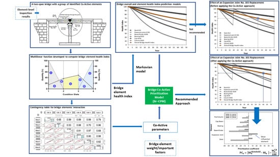
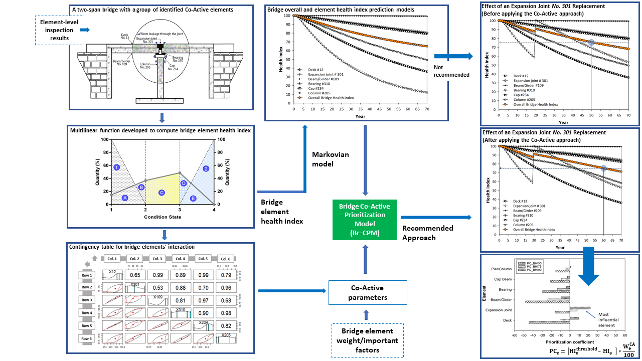
The scope and application of bridge MRR prioritization analysis largely depends on state Departments of Transportation (DOTs) bridge management program and how they measure bridge performance. The American Association of State Highway and Transportation Officials (AASHTO) sufficiency rating (SR) and National Bridge Inventory (NBI) general condition rating (GCR) among others have been routinely used as bridge performance measures since the 1970s. The AASHTO SR is a performance measure, which indicates safety, functionality, overall adequacy, and ability of a bridge to remain in service [11,12,13]. Contrary to the AASHTO SR, the NBI GCR gives condition ratings of the three major bridge components (deck, superstructure, and substructure).

While bridge performance evaluation approaches such as AASHTO SR and NBI GCR have been widely implemented, inherent deficiencies exist [14,15,16,17]. The NBI GCR approach provides information on the severity of a bridge condition in terms of the condition rating (CR) but does not provide a quantitative evaluation [14]. For example, in GCR, 310 m² bridge decks with a 150 m² and 125 m² spalling area are both classified as a CR of ‘4’ [18] on the scale of 10 (excellent). However, based on the percentage of deteriorated areas, they may be given more precise and quantitative condition scores, 3.51 and 4.49, respectively.

Recently, the Element-level Bridge Inspection [1] data has enabled a quantitative performance analysis. One of the key strengths of element level inspection, which can be performed by the visual inspection of bridges, is its ability to simultaneously capture the severity and extent of deterioration of an element [13]. As a result, BHIs are determined based on bridge elements’ conditions, which makes them effective for prioritization of MRR activities. Although element-level data result from visual inspections, they provide a numerical score based on physical quantities of each element in four condition states. The link that the health index provides between the condition and asset value allows bridge managers to translate the condition to dollar amounts. The Virginia Department of Transportation has been very successful in optimizing MRR activities and has saved millions of dollars by using bridge health index [19,20,21]. The relative importance of elements, together with their conditions, may enable state DOTs to make bridge action decisions. Hence, elements such as decks, piers, abutments, girder, and stay cables are classified as critical elements. These critical elements relatively have more significant effects on the BHI [22,23,24,25]. Identification, proper monitoring, and adequate maintenance of critical elements can help reduce elevated risks in bridges [26,27].

As the popularity of element-level inspection grows, most bridge management professionals are optimistic about its potential benefits, knowing that the bridge performance can be better assessed when detailed information is available. Yet, due to the uncertainties surrounding the determination of each element important weight, accurate predictions of BHIs remain challenging. Without a quantitative description of how critical each element is, the computation of a BHI using the broad classification of elements as critical and non-critical elements may be misleading. Studies on the application of element-level inspections indicate that the BHI, as a bridge performance measure, is better assessed by using various element important weight factors such as repair cost, reliability indices, or other agency-priority weights [8,13,28,29,30,31]. Jiang and Rens [7] suggested that element important weight factors should not be solely based on repair or replacement cost. Patidar et al. [32] used multiple factors (risk, condition, cost, and priority) to determine element weight factors. More recently, Inkoom et al. [8] analyzed element weight factors based on bridge element’s replacement costs, long-term maintenance costs, and vulnerability to natural and manmade hazards.

A few studies that account for the relationships between elements are available in the literature [33,34]. The fault tree and impact tree methods have been used to analyze how one element affects the other elements [35,36,37]. However, these methods are probability-based analyses with hypothetical quantities and did not use actual quantities measured from the Element-level Bridge Inspections. The National Cooperative Highway Research Program (NCHRP) Report 551 presents a step-by-step guide for identifying performance measures [38] but is silent on inter-dependencies among elements.

3. Methodology

This section identified and computed Co-Active parameters that influence the overall BHIs. These parameters include Co-Active correlation coefficients and collaboration factors. Contingency tables are used for determining the Co-Active correlation coefficients, which are in turn used to assess the bridge health index.

3.1. Development of Contingency Tables

As presented earlier, the existing approach for bridge MRR prioritization considers elements independently, resulting in overly conservative predictions. This section describes how contingency tables are effectively used to prioritize MRRs.

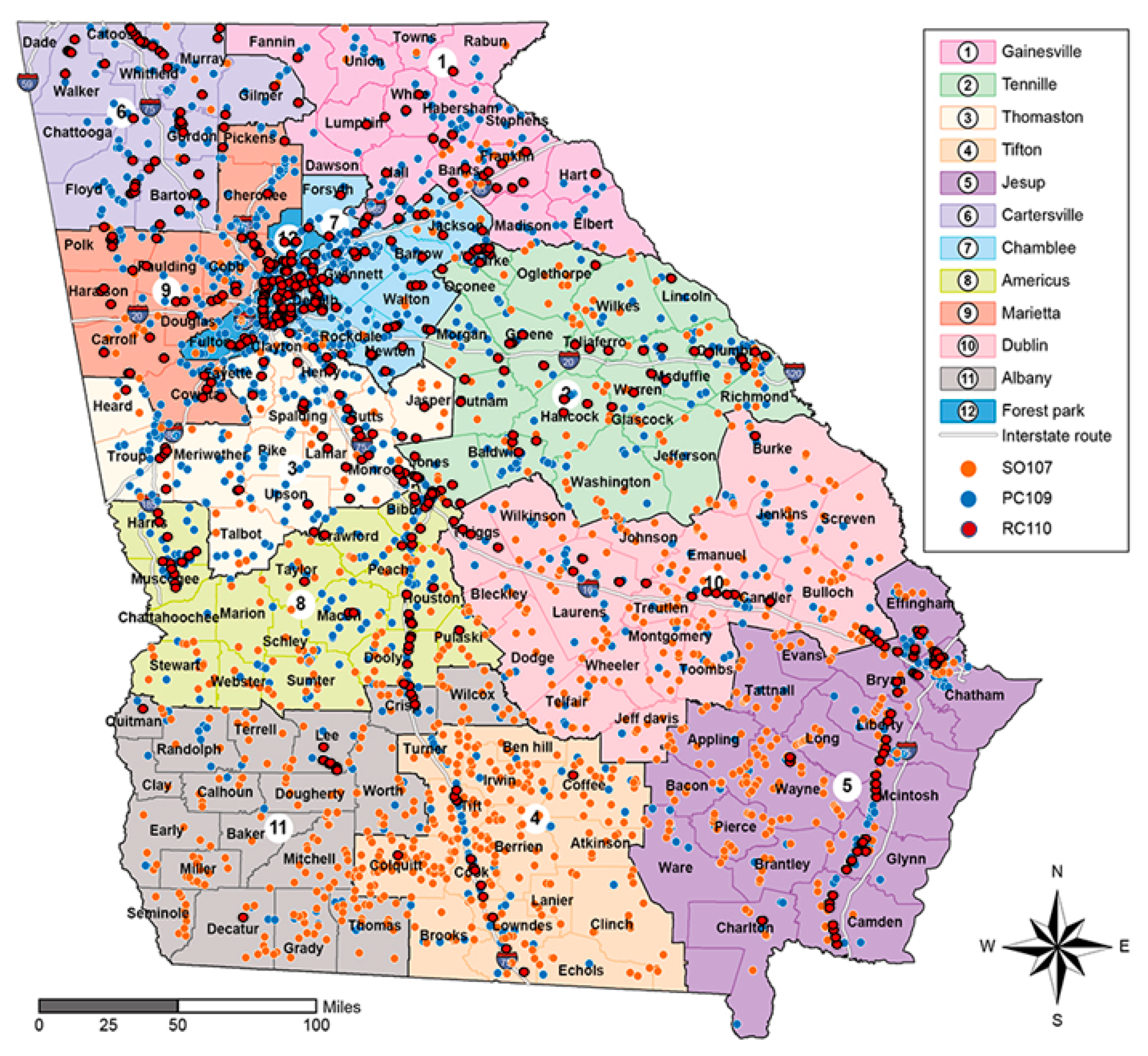
3.1.1. Identify Groups by Bridge Types

Bridge structures are usually made up of different types and number of elements due to the inherent variations. For example, a steel deck with corrugated material in a highly corrosive marine environment will deteriorate at a much faster rate than a reinforced concrete deck. Therefore, bridge groups having the same type and number of elements are identified. For this study, the three most common groups were identified among 9044 in service bridges (excluding culverts) in the state of Georgia, U.S.A.

These groups consisted of bridges, which were categorized primarily based on the type of material used for the girder/beam element:

• Steel open girder/beam bridge (SO107): This group consisted of bridges with steel open girder (I section) as the means of supporting the overlying reinforced concrete deck, and in transmitting loads from the reinforced concrete deck into the underlying substructure. There were 598 bridges in this group. The last three numbers, ‘107’, in ‘SO107’, is an element identification number for steel open girder/beam bridge element. The first two letters, ‘SO’, means steel open, added to emphasize this group and make it unique in representation.
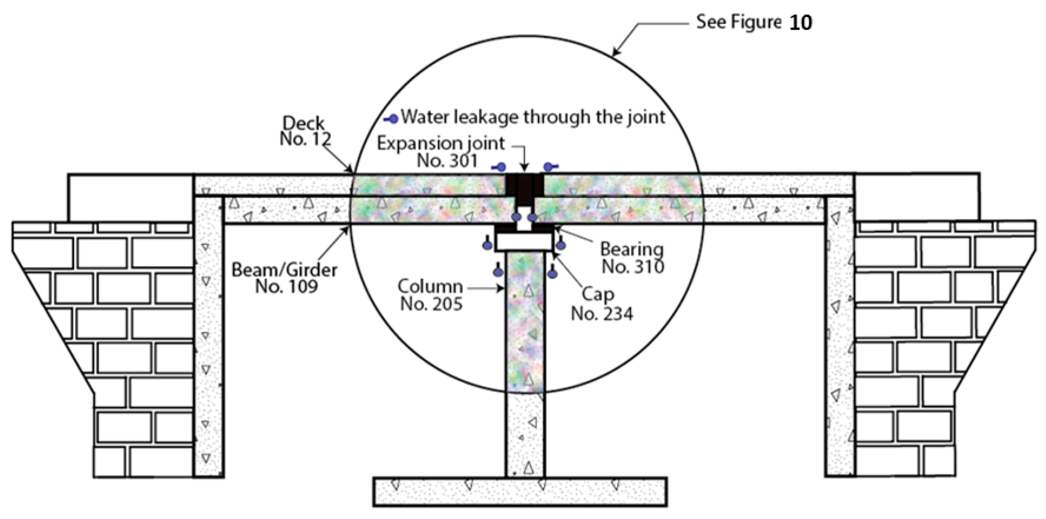
• Prestressed concrete open girder/beam bridge (PC109): In this group, each bridge contained prestressed concrete as the open girder/beam element’s material. The open girder/beam element in this bridge group performed similar functions as described in the group ‘SO107’, steel open girder/beam bridge. There were 1439 bridges in this group. Figure 2 shows a typical in-service prestressed concrete girder/beam bridge, which is the most common type in Georgia.
• Reinforced concrete open girder/beam with pile foundation bridge (RC110): Unlike the other two groups, bridges in this group contained reinforced concrete as a construction material for the open girder/beam element. In addition, each bridge contained a pile foundation. There were 1098 bridges in this group.

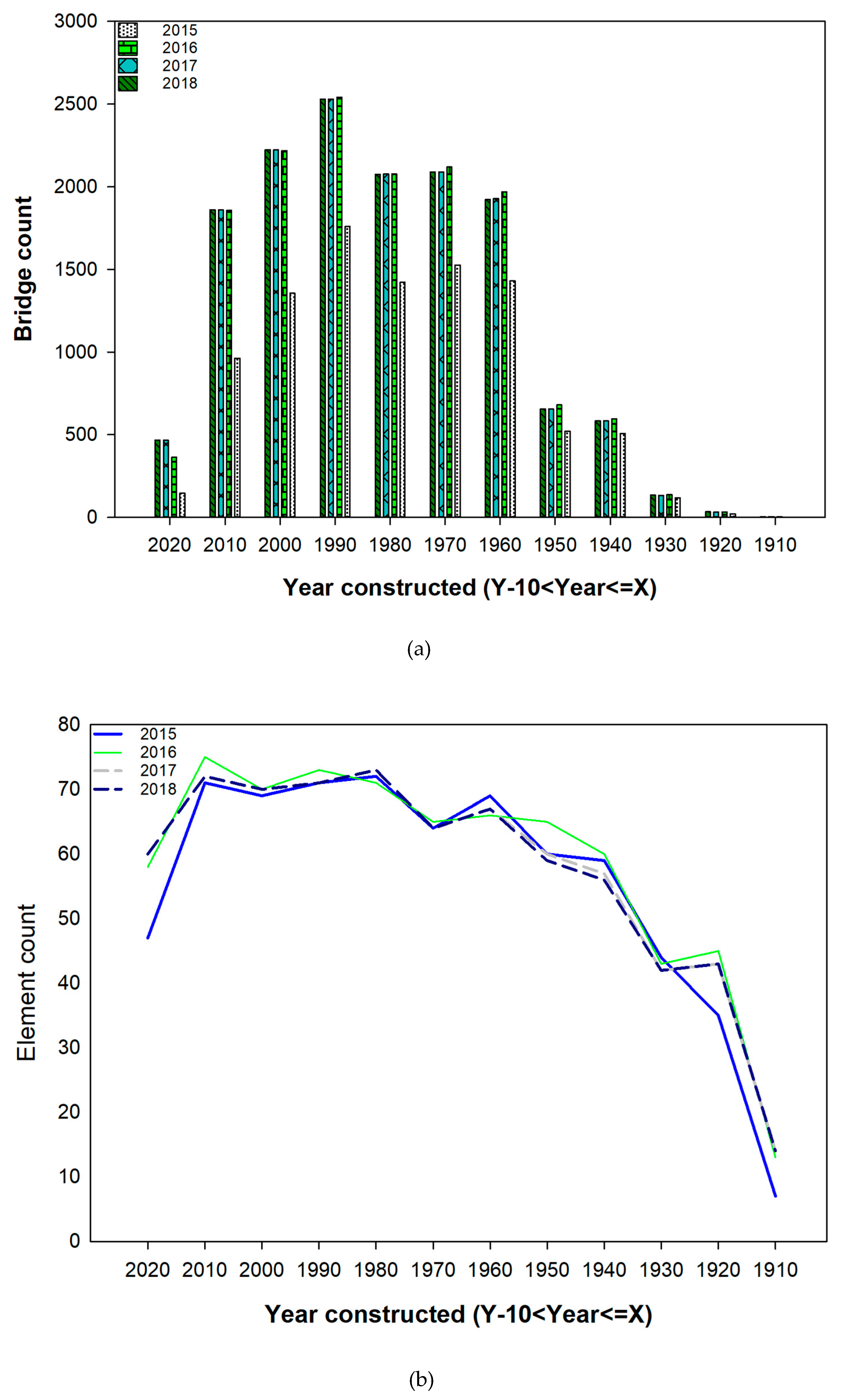
3.1.2. Create 12 Age Bins for Bridges in Each Group

Bridges were categorized by 12 age bins shown in Figure 1 because ages should affect bridge performance. While bridges in the steel open girder/beam bridge (SO107) group were evenly distributed around the southern part of Georgia, there were a cluster of bridges around Atlanta, in inspection areas 7, 9, and 12, for the other bridge groups, prestressed concrete girder/beam bridge (PC109), and reinforced concrete open girder/beam with pile foundation bridge, RC110 (Figure 3). The element health indexes by age for bridges in the first bridge group, steel open girder/beam bridge (SO107), were presented later to illustrate the procedure for determining the Co-Active parameters, which were required for the implementation of the Br-CPM. In this study, the significance of the output from the proposed Br-CPM and the prioritization coefficient (PC) is clearly shown, in terms of decision making regarding how to optimize return on investment (ROI) on element’s preventive maintenance, rehabilitation, or replacement (MRR).

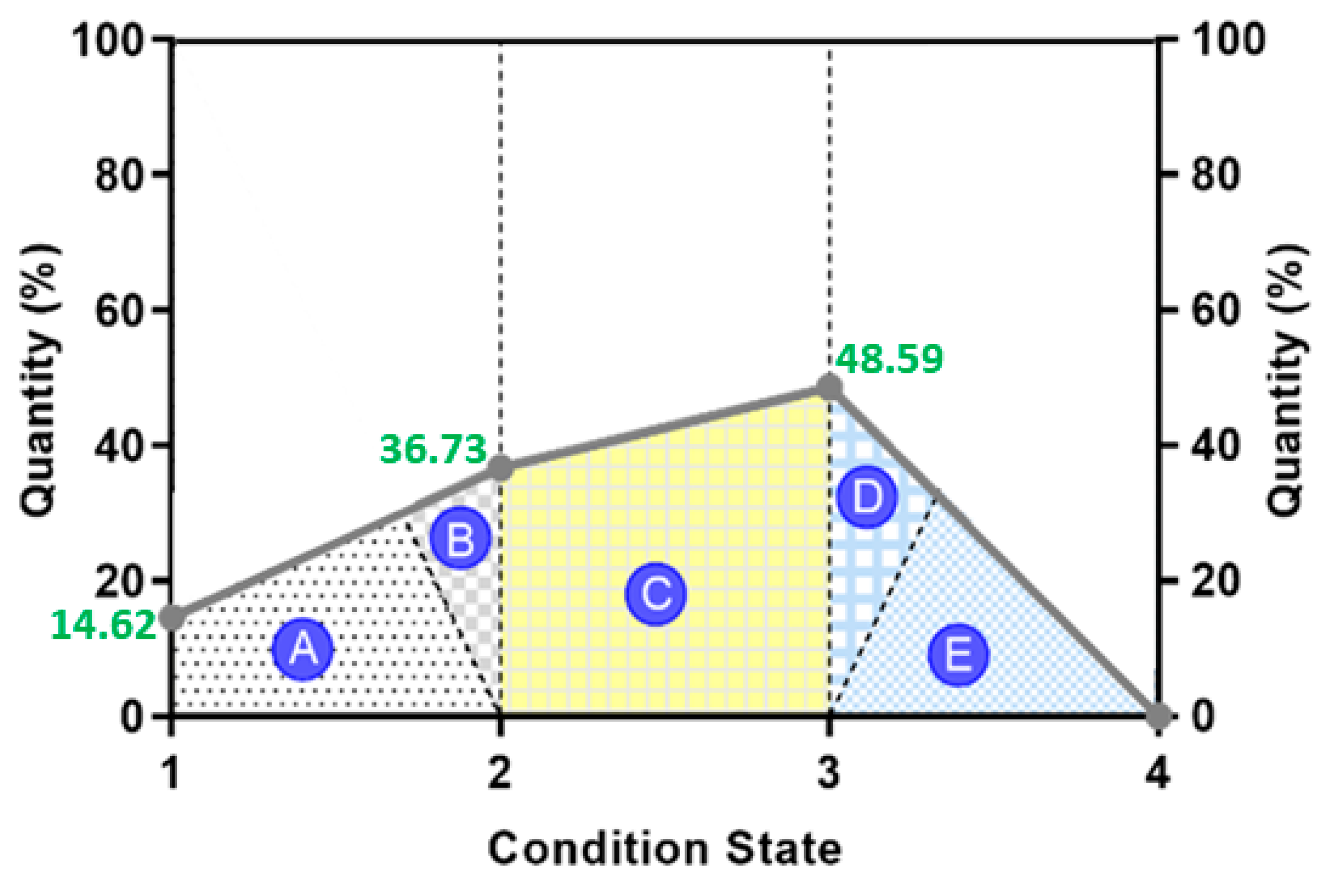
3.1.3. Compute Health Indexes for Elements in Each Age Bin

The procedure for computing element health indexes is described by the following 3 steps.

Step 1: Compute each element’s percentage quantities in 4 condition states for an age bin

Table 1. A typical element-level inspection in Georgia (reinforced concrete deck for age bin 1940).

STRUCNUM	EN	TOTAL QTY (m2)	CS1 (m2)	CS2 (m2)	CS3 (m2)	CS4 (m2)
20700220	12	310	0	264	46	0
19950080	12	67	67	0	0	0
28500340	12	1526	0	0	1526	0
19950740	12	42	0	42	0	0
26300160	12	499	487	11	0	0
6300860	12	191	0	0	191	0
19950490	12	36	0	36	0	0
19900470	12	328	0	317	10	0
20700210	12	310	0	294	16	0
25550440	12	85	0	85	0	0
19950520	12	279	0	0	279	0
19950680	12	80	0	80	0	0
17100110	12	232	0	231	0	0
19950620	12	72	72	0	0	0
20700140	12	226	0	213	13	0
Row A—Quantity Sum		4283(a)	626(b)	1573(c)	2081(d)	0(e)
*Row B—% Quantity		100	14.62(f)	36.73(g)	48.59(h)	0(i)

Notes: STRUCNUM = structure number; EN = element number; TOTALQTY = total quantity; CS1 = condition state 1 (good); CS2 = condition state 2 (fair); CS3 = condition state 3(poor); CS4 = condition state 4 (severe); *The last row, “Row B”, corresponds to age-bin 1940 in Table 2.

shows the reinforced concrete deck element (No. 12) condition states (CSs) for 15 bridges in age bin 1940. In the table, there were four CSs, with one and four being the good and severe conditions, respectively. In each CS, the area of distress was quantified. The quantities in each CS were combined to determine the total quantity for the 15 bridges as shown in the “Row A”, at the bottom of Table 1. The last row, “Row B”, presents the percentage quantities in each CS. They were determined by taking the quantities in each CS and dividing by the total quantity, 4283 m².

Step 2: Compute each element’s percentage quantities in 4 condition states for all age bins

Repeating the process described in Step 1, each element’s % quantities were calculated for a group of bridges in each age bin as shown in

Table 2. Percentage quantities for element 12 (reinforced concrete deck).

Age-bin	% Quantities in each condition state
	1	2	3	4
	(Good)	(Fair)	(Poor)	(Severe)
2020	99.52	0.48	0	0
2010	90.39	8.10	1.51	0
2000	76.17	22.27	1.56	0
1990	75.41	21.26	3.33	0
1980	60.19	39.70	0.11	0
1970	25.61	62.58	11.81	0
1960	18.57	70.63	10.8	0
1950	24.77	54.96	20.28	0
** 1940	14.62	36.73	48.59	0	(See “Row B”, in Table 1)
1930	0	0	0	0
1920	0	0	0	0
1910	0	0	0	0

Notes: ** This row was obtained from Table 1.

.

Step 3: Compute element health indices for all age bins

This study utilized a multi-linear function shown in Figure 4 and computed the element HI. The multi-linear function was defined by the element’s percentage quantities (see Table 2) and gave

Table 3. Computation of element 12 health indexes, HI₁₂ (reinforced concrete deck).

(a) Age-bin	Aggregated Percentage Quantity					HI12
	(Area ‘A’)	(Area ‘B’)	(Area ‘C’)	(Area ‘D’)	(Area ‘E’)
2020	49.90	0.10	0.20	0	0	99.80
2010	47.40	1.90	4.80	0	0.70	96.20
2000	43.80	5.40	11.90	0	0.80	91.40
1990	43.40	4.90	12.30	0.10	1.60	90.50
1980	40.00	9.90	19.90	0	0.10	86.40
1970	29.80	14.30	37.20	0.60	5.30	70.50
1960	28.20	16.40	40.70	0.50	4.90	68.50
1950	28.30	11.60	37.60	1.70	8.40	67.00
1940	20.20	5.50	42.70	8	16.40	51.20
1930	0	0	0	0	0	0
1920	0	0	0	0	0	0
1910	0	0	0	0	0	0
(b) Weighing factors [8]	2.0	0.24	0.20	0.12	0.0

as output. For example, the element’s percentage quantities in each age bin in Table 2 (e.g., 14.62, 36.73, 48.59, and 0, in age bin 1940) was used to characterize the multilinear function with 4 points shown in Figure 4. Table 3 summaries the numerical values of the five areas (A, B, C, D, and E) shown in Figure 4.

In Table 3, the product of each area (A through E) and its corresponding weighting factor [8] (see part ’b’) was calculated to determine HI for element 12 (reinforced concrete bridge deck) in the last column. For example, the HI for a group of reinforced concrete decks in age bin 1940 was 51.20 $(=(20.20\times 2.0)+(5.50\times 0.24)+(42.70\times 0.20)+(8\times 0.12)+(16.40\times 0.0\left)\right)$.

3.1.4. Develop Deterioration Prediction for Each Element

An age-bin analysis approach, utilizing element HIs computed in Step 3 of Section 3.1.3 (Table 3), was used to develop deterioration predictions presented in this study using the Markov-chain method [39]. The Markov-chain method requires condition state (CS) transition probabilities in each element and bridge. For each transition probability matrix, three unknowns ($P_{11},\dots P_{33}$) were estimated by minimizing the sum of errors between predicted and aggregated health indexes [40]:

$$\widehat{P}=min\left[{\displaystyle \sum }_{j=1}^N|y_{n,j}-R_{p,n}|\right]\mathrm{subject}\mathrm{to}0\le p_{ii}\le 1\mathrm{for}i=1,2,3,\dots ,ns$$

(1)

where, $min$ denotes minimization; N denotes the number of bridges or elements belonging to a subset; $ns$ is the number of condition states; $y_{n,j}$ is the observed (aggregated) health index at an $n\mathrm{th}$ age-bin of $j$th bridge; and $R_{p,n}$ is the predicted health index.

As a result of the process described from this section, HIs of bridge elements were described as a function of time. That is, deterioration models, which describe HIs as a function of time, were developed for each bridge element [41].

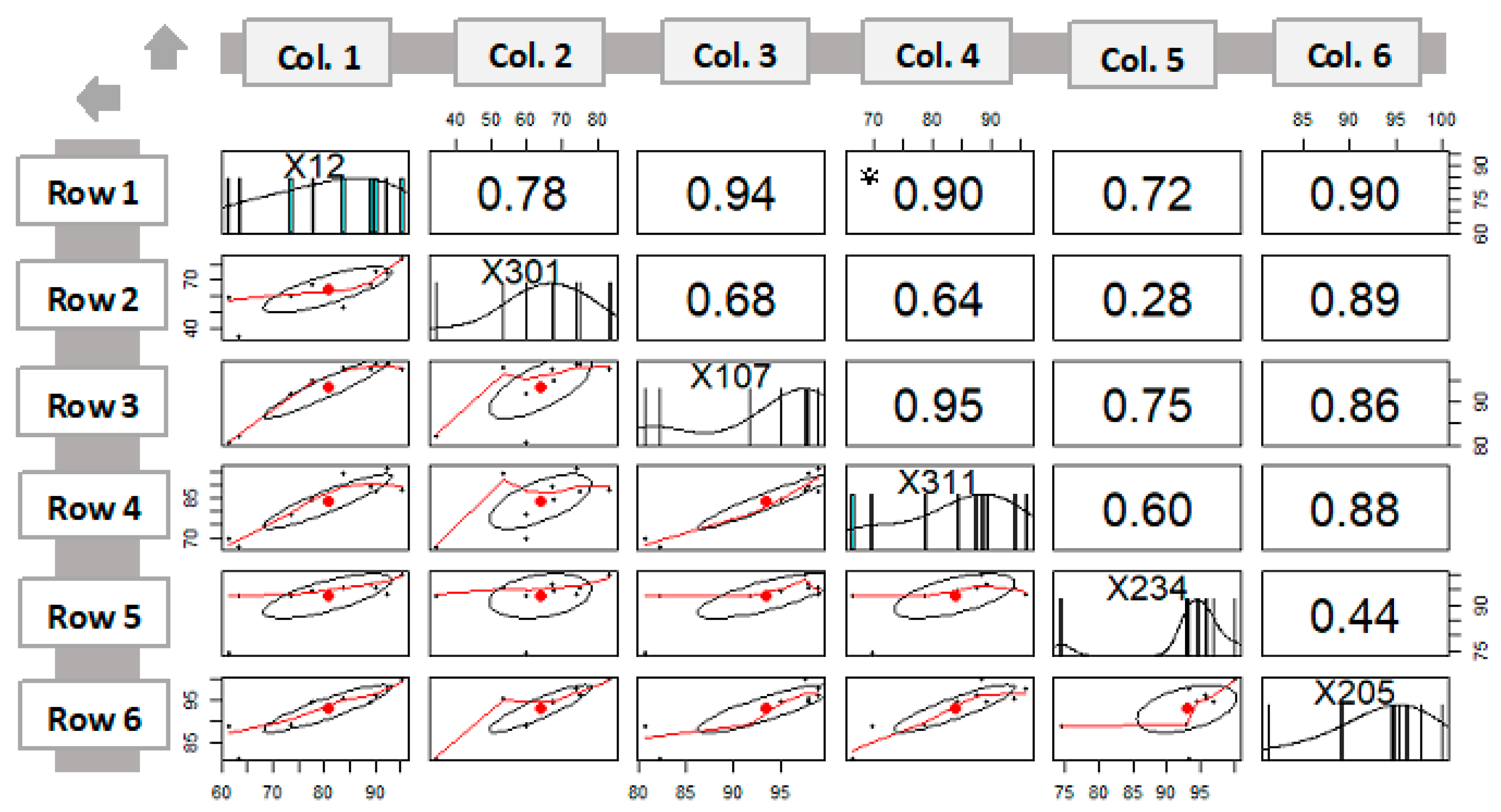
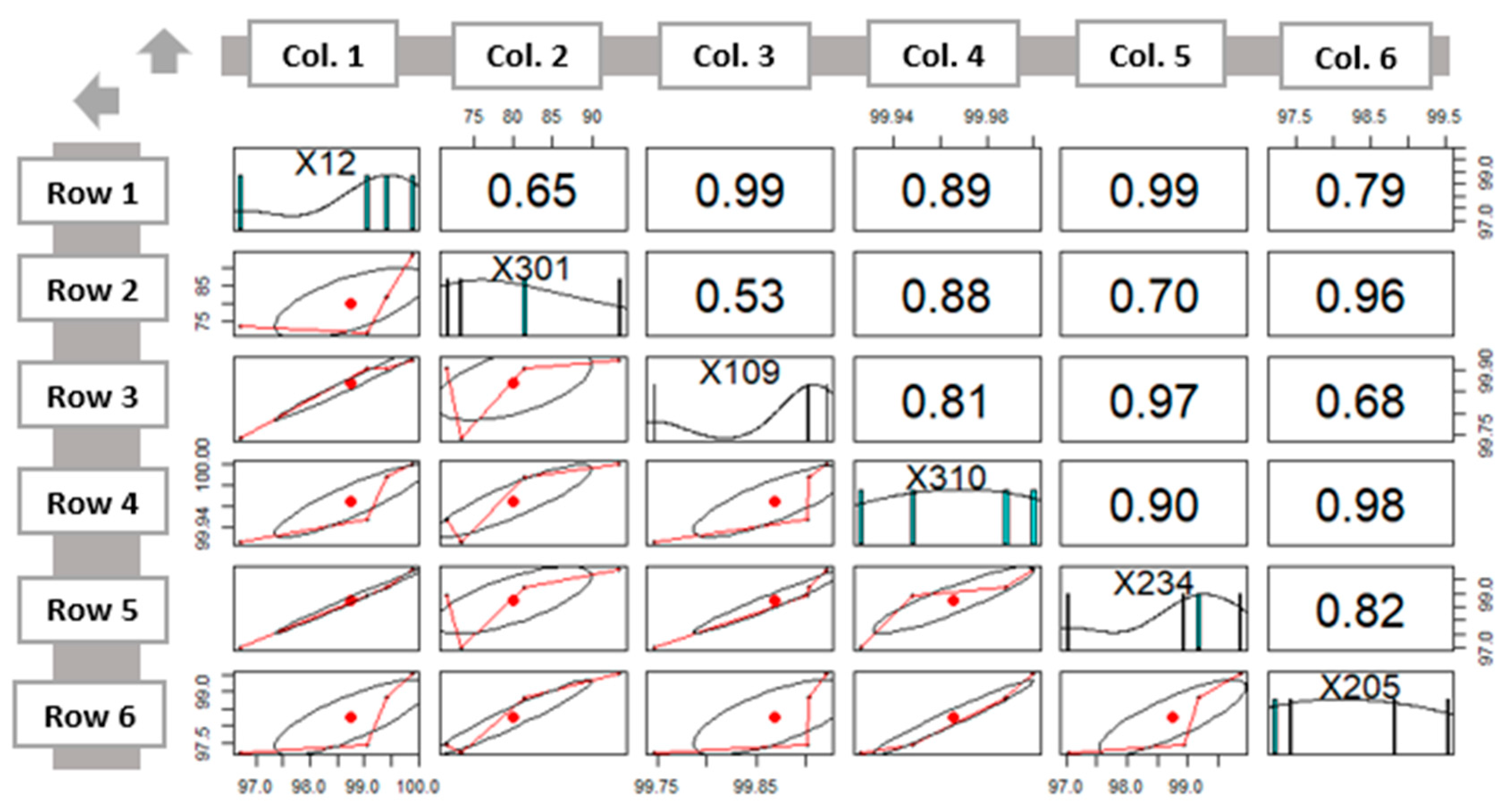
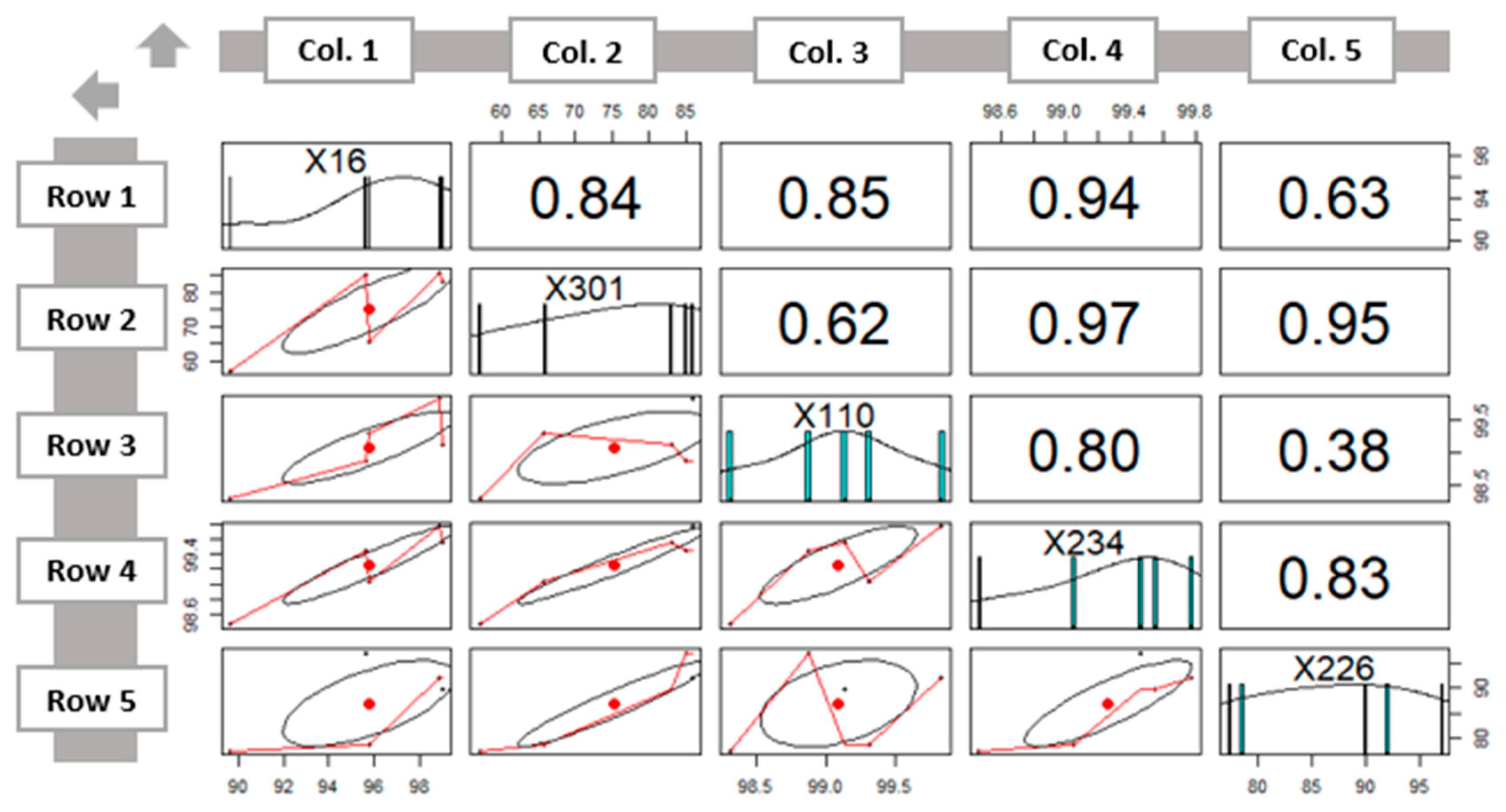
3.1.5. Develop Contingency Tables and Determine Element Co-Active Coefficients

A contingency table was developed to provide interactions among Co-Active elements, describing correlation coefficients for pairs of Co-Active elements. It is expressed in a 2 × 2 table. Equation (2) defines the Co-Active correlation coefficients. It measures how much one element HIs, ‘X’, affects the other element HIs, ‘Y’, based on the Pearson correlation coefficient [42].

$$\mathsf{\rho }\left(\mathrm{X},\mathrm{Y}\right)=\frac{\mathrm{Cov}\left[\mathrm{X},\mathrm{Y}\right]}{\sqrt{{\mathsf{\sigma }}^2\left[\mathrm{X}\right]{\mathsf{\sigma }}^2\left[\mathrm{Y}\right]}}$$

(2)

where, $\mathrm{Cov}\left[\mathrm{X},\mathrm{Y}\right]$ is the covariance between the two elements’ HIs and ${\sigma }^2\left[\mathrm{X}\right],{\sigma }^2\left[\mathrm{Y}\right]$ denotes their variances in each age bin. In the case of non-Co-Active elements, $\mathsf{\rho }\left(\mathrm{X},\mathrm{Y}\right)=0$. since $\mathrm{Cov}\left[\mathrm{X},\mathrm{Y}\right]=0$.

3.2. Computation of Element Collobaration Factors

3.2.1. Existing Element Weight Factors

This study adopted the element weight factors recommended by Sobanjo and Thompson [10]. In their approach, element weight factors are determined based on element replacement unit costs, element long-term unit costs, and more.

3.2.2. Collaboration Factors

The collaboration factors are defined by Equation (3) and used for a prioritization model (see Section 5). With the ‘${\mathrm{N}}_{\mathrm{e}}^{\mathrm{CA}}$’ number of Co-Active elements, the number of 2-element interactions is $\frac{1}{2}({\mathrm{N}}_{\mathrm{e}}^{\mathrm{CA}}!/\left({\mathrm{N}}_{\mathrm{e}}^{\mathrm{CA}}-2\right)!)+{\mathrm{N}}_{\mathrm{e}}^{\mathrm{CA}}$. Collaboration factors were determined by multiplying the Co-Active coefficients by the (importance) weight factors developed by Sobanjo and Thompson [10] including the cost and risk. They were used in the neighboring state, Florida, to weigh elements and determine the overall BHI. This collaboration factor plays an important role for decision making at discrete times (see Section 5.1).

$${\mathrm{W}}_{\mathrm{e}}^{\mathrm{C}}={\displaystyle \sum }_{\mathrm{i}}^{{\mathrm{N}}_{\mathrm{e}}^{\mathrm{CA}}}{\mathsf{\rho }}_{\mathrm{e}}^{\mathrm{CA}}{\mathrm{W}}_{\mathrm{e}}$$

(3)

where,

• ${\mathrm{W}}_{\mathrm{e}}^{\mathrm{C}}$ = Collaboration factor,
• ${\mathrm{W}}_{\mathrm{e}}$ = Weight factor [10] given to element, ‘e’,
• ${\mathsf{\rho }}_{\mathrm{e}}^{\mathrm{CA}}$ = Co-Active correlation coefficient between two elements’ HIs (from Equation (2)),
• ${\mathrm{N}}_{\mathrm{e}}^{\mathrm{CA}}$ = the number of Co-Active elements.

3.3. Bridge Health Index Assessment

Figure 5 is a flowchart showing how one element’s change in HI affects the other elements. For example, when an expansion joint’s HI changed from 60 to 100 in Year 20, it affected HIs of the other elements (e.g., cap beam, bearing, column, and girder) due to the proposed Co-active model. The number in each arrow shows the Co-Active correlation coefficient between the expansion joint and each element. The overall BHIs were determined by a weighted average of element HIs.

4. Analytical Investigation of Co-Active Elements in Three Bridge Groups

This section presents the Co-Active coefficients, obtained from the contingency tables, and collaboration factors for the three major bridge groups identified in this study.

4.1. Contingency Table for Co-Active Coefficients

Table 4. Element health indexes by age for bridges in the ‘SO107’ group.

Age-bin	Deck	Expansion Joint	Beam/Girder	Bearing	Cap Beam	Pier/Column
2020	95.26	83.58	97.65	88.41	99.92	100.00
2010	92.30	74.34	98.92	95.95	93.28	97.68
2000	90.15	75.05	98.97	87.42	95.67	96.20
1990	83.73	53.36	98.02	93.99	95.79	95.34
1980	89.15	67.42	97.87	89.25	96.87	94.82
1970	77.76	67.50	95.03	84.22	94.57	94.60
1960	73.51	60.03	91.82	78.77	92.86	89.23
1950	63.32	34.68	82.26	66.45	93.14	81.31
1940	61.28	59.72	80.71	69.66	74.41	89.06

lists bridge elements by age for bridges in the steel open girder/beam bridge (SO107) group. They were determined by the methodology described in Section 3.1.5. Figure 6 shows the contingency table representing Co-Active coefficients for Co-Active elements in the group ‘SO107’ bridges. The small graphs in Figure 6 below the diagonal were bivariate scatter plots of two elements’ health indices, which were used for the calculation of the Co-Active coefficients. Each graph shows a relationship (e.g., a linear trend) between two elements.

For example, the Co-Active coefficient in “Row 1”, “Col. 4”, in Figure 6 (designated as ‘A’, shown in

Table 5. Co-Active prioritization parameters in the ‘SO107’ group.

(a) On the element below	The Effect of the Following Element’s Condition Change
	Deck	Expansion Joint	Beam/Girder	Bearing	Cap Beam	Pier/Column
Deck	1.00
Expansion Joint	0.78	1.00
Beam/Girder	0.94	0.68	1.00
Bearing [a] =	‘A’ = 0.90	0.64	0.95	1.00
Cap Beam	0.72	0.28	0.75	0.60	1.00
Pier/Column	0.90	0.89	0.86	0.88	0.44	1.00
(b) Aggregated Co-Active coefficient
	5.24 (Rank 1)	3.49 (Rank 2)	3.56 (Rank 3)	2.48	1.44	1.00
(c) Importance weight [10] factor, [c]=
	25.00 (Rank 3)	12.00	49.00 (Rank 1)	12.00	13.00	40.00 (Rank 2)
(d) Collaboration factor = [c][a]
	136.58 (Rank 1)	92.24 (Rank 3)	104.55 (Rank 2)	55.00	30.60	40.00

) was calculated by Equation (3).

$$\mathsf{\rho }\left(\mathrm{No}.12,\mathrm{No}.311\right)=\frac{\mathrm{Cov}[\mathrm{HI}12,\mathrm{HI}311]}{\sqrt{{\mathsf{\sigma }}^2\left[\mathrm{HI}12\right]{\mathsf{\sigma }}^2\left[\mathrm{HI}311\right]}}=0.90$$

(4)

where, $\mathrm{HI}12$ and $\mathrm{HI}311$ represent the health indexes of deck and bearing elements, respectively. For example, HI12 = [95.26, 92.30, 90.15, 83.73, 89.15, 77.76, 73.51, 63.32, 61.28] and HI311 = [88.41, 95.95, 87.42, 93.99, 89.25, 84.22, 78.77, 66.45, 69.66] come from the second and fifth columns of Table 4.

Figure 7 and Figure 8 show the contingency tables for the Co-Active elements in the other two groups, PC109 and RC110.

The aggregated Co-Active coefficient (see part ‘(b)’ of Table 5) for each element was determined by combining all coefficients in each column. For example, an aggregated Co-Active coefficient for the reinforced concrete deck was 5.24 (= 1.00 + 0.78 + 0.94 + 0.90 + 0.72 + 0.90).

4.2. Collaboration Factors

Table 5 shows the Co-Active coefficients and collaboration factors calculated for the six Co-Active elements in the group ‘SO107’ bridges. The collaboration factor was computed as the product of weight factors [10] and Co-Active coefficient for each element (see part ‘(d)’ of Table 5). This process primarily applies weight factors based on relative costs of elements and inter-dependency that exists among them. For example, the collaboration factor for the reinforced concrete deck was 136.58 $\left[=\left(1.00\times 25\right)+\left(0.78\times 12\right)+\left(0.94\times 49\right)+\left(0.90\times 12\right)+\left(0.72\times 13\right)+\left(0.90\times 40\right)\right]$.

Table 6. Co-Active prioritization parameters in the ‘PC109’ group.

On the element below	The Effect of the Following Element’s Condition Change
	Deck	Expansion Joint	Beam/Girder	Bearing	Cap Beam	Pier/Column
Deck	1.00
Expansion Joint	0.65	1.00
Beam/Girder	0.99	0.53	1.00
Bearing	0.89	0.88	0.81	1.00
Cap Beam	0.99	0.70	0.97	0.90	1.00
Pier/Column	0.79	‘B’ = 0.96	0.68	0.98	0.82	1.00
(b) Aggregated Co-Active coefficient
	5.31 (Rank 1)	4.07 (Rank 2)	3.46 (Rank 3)	2.88	1.82	1.00
(c) Importance weight [10] factor
	25.00 (Rank 3)	12.00	46.00 (Rank 1)	13.00	13.00	40.00 (Rank 2)
(d) Collaboration factor
	134.38 (Rank 1)	95.32 (Rank 3)	96.34 (Rank 2)	63.90	45.80	40.00

and

Table 7. Co-Active prioritization parameters in ‘RC110’ group.

(a) On the Element Below	The Effect of the Following Element’s Condition Change
	Deck	Expansion Joint	Beam/Girder	Cap Beam	Pile
Deck	1.00
Expansion Joint	0.84	1.00
Beam/Girder	0.85	0.62	1.00
Cap Beam	0.94	0.97	0.80	1.00
Pile	0.63	0.95	0.38	0.83	1.00
(b) Aggregated Co-Active coefficient
	4.26 (Rank 1)	3.54 (Rank 2)	2.18 (Rank 3)	1.83	1.00
(c) Importance weight [10] factor
	25.00 (Rank 2)	12.00	33.00 (Rank 1)	13.00	17.00 (Rank 3)
(d) Collaboration factor
	86.06 (Rank 1)	61.22 (Rank 2)	49.86 (Rank 3)	27.11	17.00

show the Co-Active prioritization parameters in the other two groups, PC109 and RC110. Element ranking changes when Co-Active coefficients were considered in conjunction with importance weight factors (part ‘(d)’ of Table 5, Table 6 and Table 7).

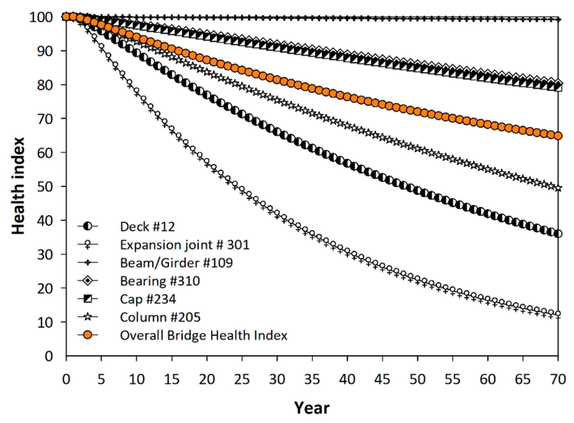
4.3. Effect of Co-Active Elements on the Bridge Health Index

A bridge generally consists of 30–80 elements. In order to analyze data from the recently mandated Element-Level Bridge Inspection program, transportation agencies in the U.S. will need to calculate a Bridge Health Index (BHI). This is a weighted average measure of the elements’ conditions. To illustrate how the proposed Co-Active model works, 1439 bridges from the Georgia Element-Level Bridge Inspection results, representing the group ‘PC109’, prestressed concrete open girder/beam bridges, were investigated (see Figure 9 and Figure 10). Group PC109 was selected for the Co-Active model because it was the most dominant bridge group in Georgia. The effect of collaboration factors for the ‘PC109’ group is presented in the following sub-section, ‘Results.’ However, all groups were analyzed in the following section, “Analysis and interpretation of results and implementation”.

Figure 10 shows the complex interactions that existed among the six Co-Active elements in the prestressed concrete open girder/beam bridge (PC109) group. The arrow originating from one bridge element (e.g., expansion joint) to another one (e.g., bearing) shows that the long-term performance of bearing was dependent on the expansion joint’s performance, based on the computed Co-Active coefficients shown in Table 6. In other words, if the condition of the expansion joint deteriorates/appreciates, it is likely going to affect the bearing element’s long-term performance. Furthermore, the four arrows originating from the expansion joint show that the long-term performance of bearing, cap beam, and column were dependent on expansion joint’s deterioration/appreciation rates. The arrows shown in the figure are given in different colors to indicate the rates at which changes in the condition of an element affects the other dependent bridge elements.

For example, the green color arrows show the most dominant inter-dependent relationship between pairs of Co-Active elements, having Co-Active coefficients between 0.90 and 1.00. Thus, the green color arrows originating from the expansion joint shows that the long-term performance of the pier/column was most dependent on the changes in the condition of the expansion joint. By investing in the expansion joint’s MRR, the long-term performance of other elements (beam/girder, bearing, cap, and column) also improves over time.

Figure 11 shows the deterioration models (or time-history of HIs) for the six Co-Active elements and an overall bridge. The deterioration models were developed using the Markovian modeling approach [43]. In this study, the overall BHI represents HI predictions for bridges that pertained the six elements. In Georgia for instance, at least 1439 bridges pertained these six elements. The elements’ deterioration models were aggregated to obtain an overall bridge model using element weight factors. For each element deterioration model, there were year-to-year depreciation factors (DFs) for each element’s HIs (i.e., the element’s deterioration rates). For example, if the reinforced concrete column’s HIs were 89.06 and 88.16 in the Years 2014 and 2015, respectively, the Year 2014–to–2015 DF was 0.01 (= (89.06–88.16)/89.06).

When one of Co-Active elements is maintained, rehabilitated, or replaced (MRR), it affects the DFs for the other Co-Active elements, the elements’ HIs, and the overall BHI. However, the extent to which the MRR of a Co-Active element affects the other elements’ DFs is quantified by ${\mathrm{AF}}_{\mathrm{e}}^{\mathrm{acting}}·{\mathsf{\rho }}_{\mathrm{e}}^{\mathrm{CA}}$, where ${\mathrm{AF}}_{\mathrm{e}}^{\mathrm{acting}}$ is the appreciation factor calculated for an element (e.g., expansion joint) being maintained, repaired, and rehabilitated. ${\mathrm{AF}}_{\mathrm{e}}^{\mathrm{acting}}$ is 2.0 if an element HI increases from 50 to 100 and 5.0 if it increases from 20 to 100. ${\mathsf{\rho }}_{\mathrm{e}}^{\mathrm{CA}}$ is the Co-Active coefficient between the acting element (e.g., expansion joint) and its co-active elements (e.g., column). The depreciation factor for the affected element (e.g., column) decreases due to the Co-Active relationship with the expansion joint:

$${\mathrm{DF}}_{\mathrm{e}}^{\mathrm{affcted}}(1-{\mathrm{AF}}_{\mathrm{e}}^{\mathrm{acting}}·{\mathsf{\rho }}_{\mathrm{e}}^{\mathrm{CA}})$$

(5)

To illustrate how this equation works, a case study, involving the replacement of an expansion joint in the Year 20 (threshold element HI is 75), was considered. The following sub-section presents the results, which show the effects of Co-Active elements on the bridge performance over time. Comparison of the analysis results (with and without the application of the Co-Active model) was also presented. The purpose of this comparison was to determine the impact of the Co-Active model, in terms of projected overall BHI obtained after bridge element’s repair or replacement.

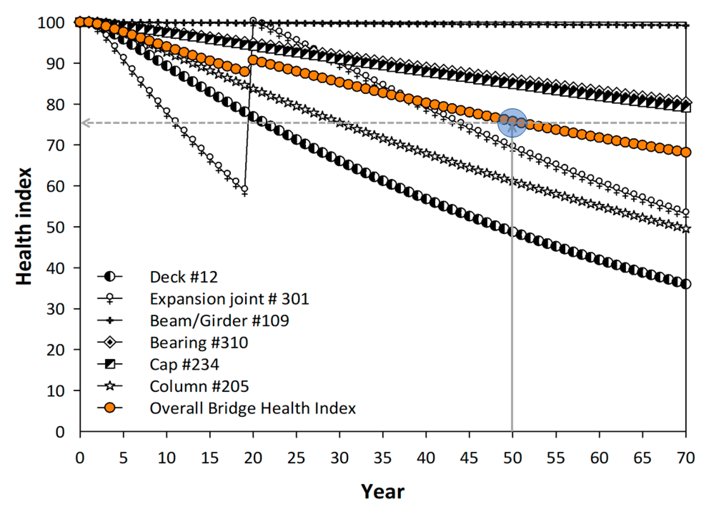
4.3.1. Results Obtained without Co-Active Model

Figure 12 shows the overall bridge and element HIs, before applying the Co-Active model, when an expansion joint was replaced in Year 20. The HI of 100 indicates an excellent condition.

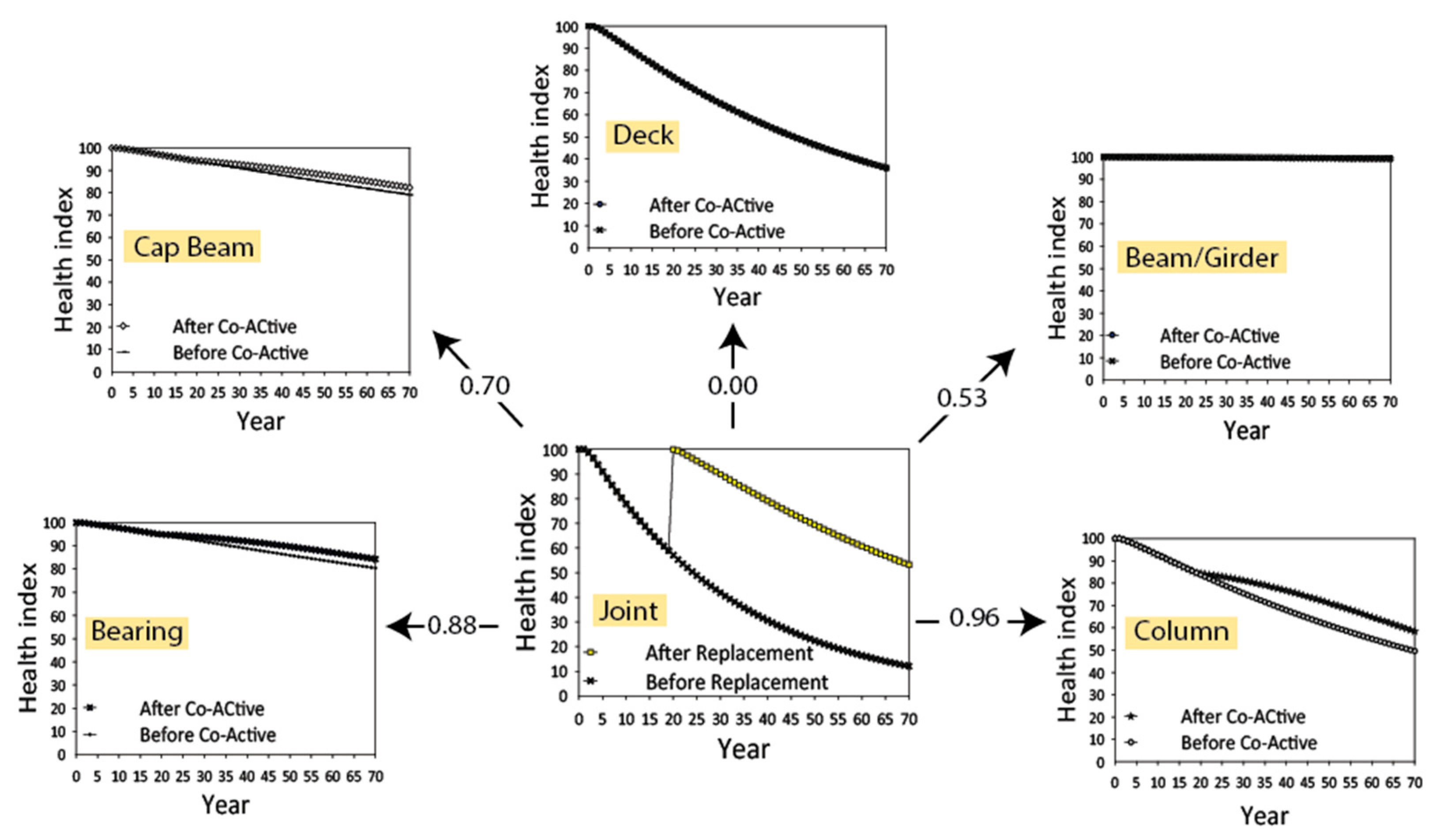
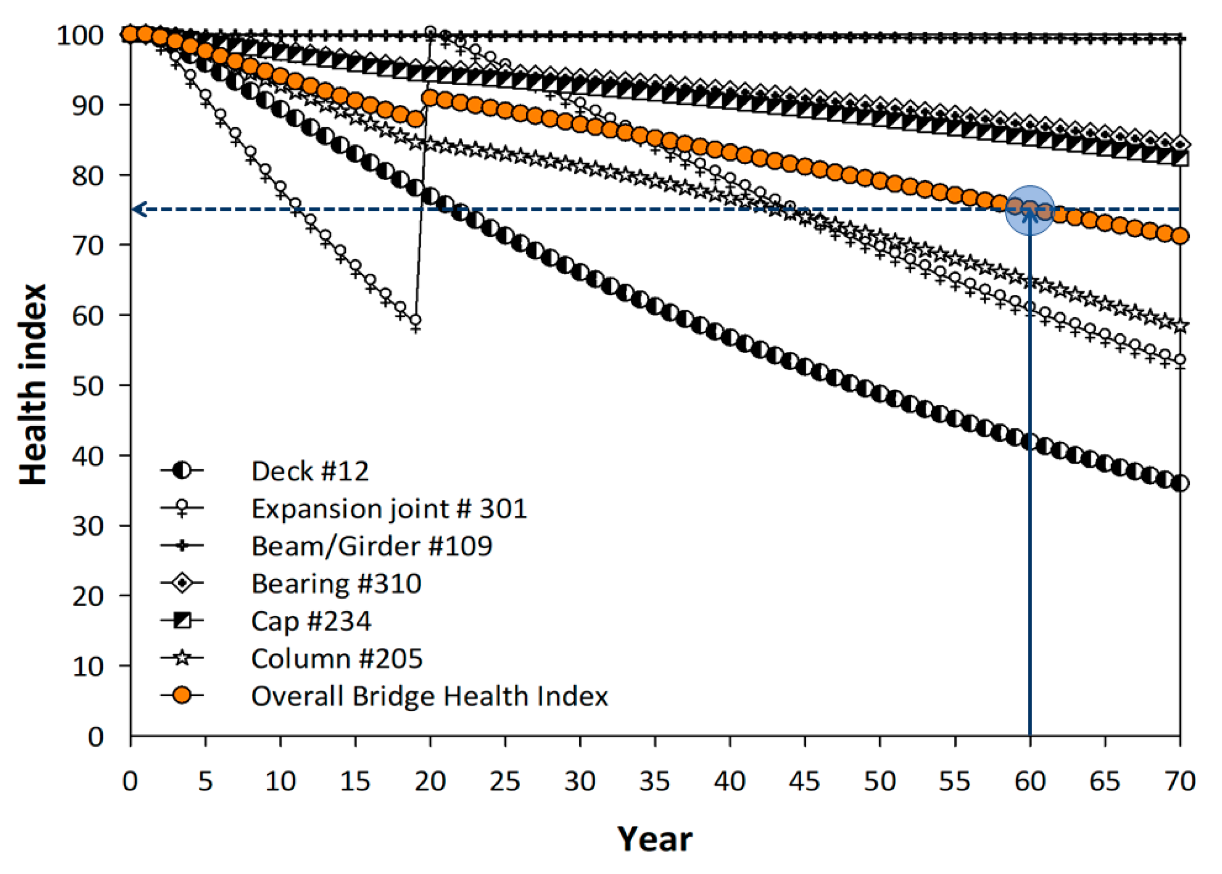
4.3.2. Results Obtained with Co-Active Model

Figure 13 shows the overall bridge and element HIs, after applying the Co-Active model, when an expansion joint is replaced in Year 20. ${\mathrm{DF}}_{\mathrm{e}}^{\mathrm{affcted}}$ represents the initial slope of an affected element (e.g., bearing) in the depreciation model, which is reduced by ${\mathrm{AF}}_{\mathrm{e}}^{\mathrm{acting}}·{\mathsf{\rho }}_{\mathrm{e}}^{\mathrm{CA}}$ computed from the expansion joint’s HI change and Co-Active relationship with the affected elements (e.g., bearing and cap) shown in Figure 13.

The Co-Active model considers the effects of the complex systems of interaction, which is a function of key parameters that define elements’ inter-dependent relationships, on the BHIs over time. By using the Co-Active model, bridge performance life improved from 50 to 60 years, an increase of 20% (see Figure 12 and Figure 13). The 20% increase in the bridge performance life indicates the indirect effects of an expansion joint’s replacement on the other elements’ performance, which the current methodology in Figure 12 was unable to capture.

When one of the Co-Active elements (e.g., an expansion joint) was replaced or repaired, its overall bridge performance improved. However, after the replacement or repair, the expansion joint’s HI, in fact, decreased over time as it deteriorated. Consequently, the Co-Active coefficients should vary as a function of time and have a diminishing effect on the overall bridge HI. Therefore, the effect of Co-Active coefficient on the elements’ HIs and overall BHI predictions was dependent on three main factors:

• The year in which a Co-Active element was maintained, rehabilitated, or replaced (MRR).
• The condition of a Co-Active element (i.e., an element HI) before MRR and the type of MRR action. The more the performance gap (i.e., the difference between an element’s HI before and after MRR), the more influential the element’s MRR was on the HI predictions.
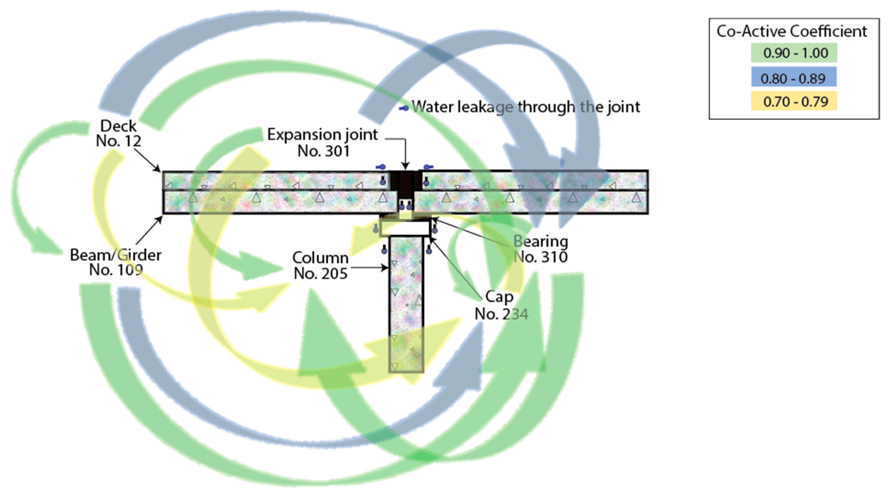
• The inter-dependencies among the Co-Active elements. The elements’ inter-dependency was a function of their Co-Active coefficients. The higher the value of an element Co-Active coefficient, the more dependent the element was.

5. Analysis and Interpretation of Results and Implementation

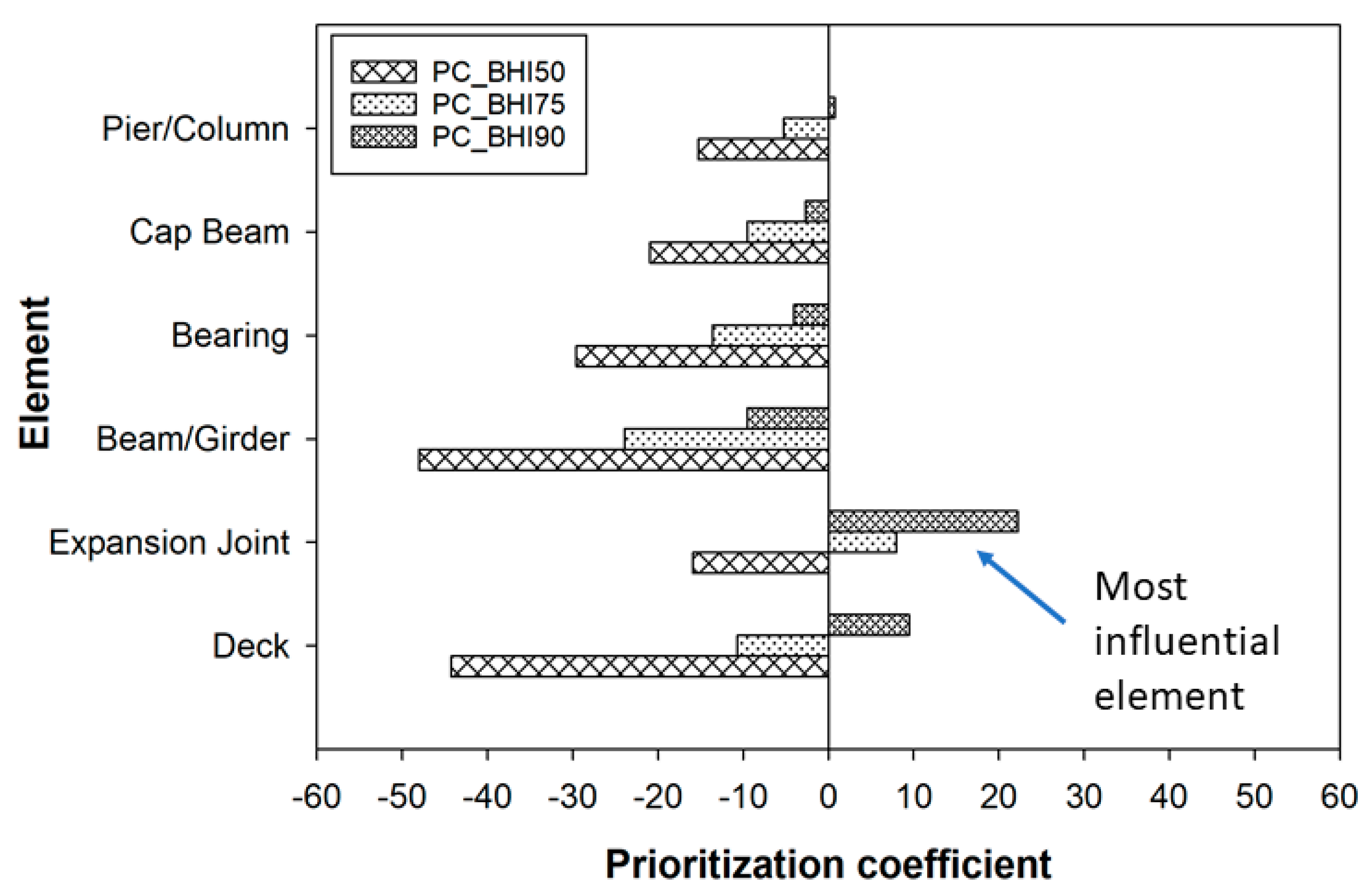
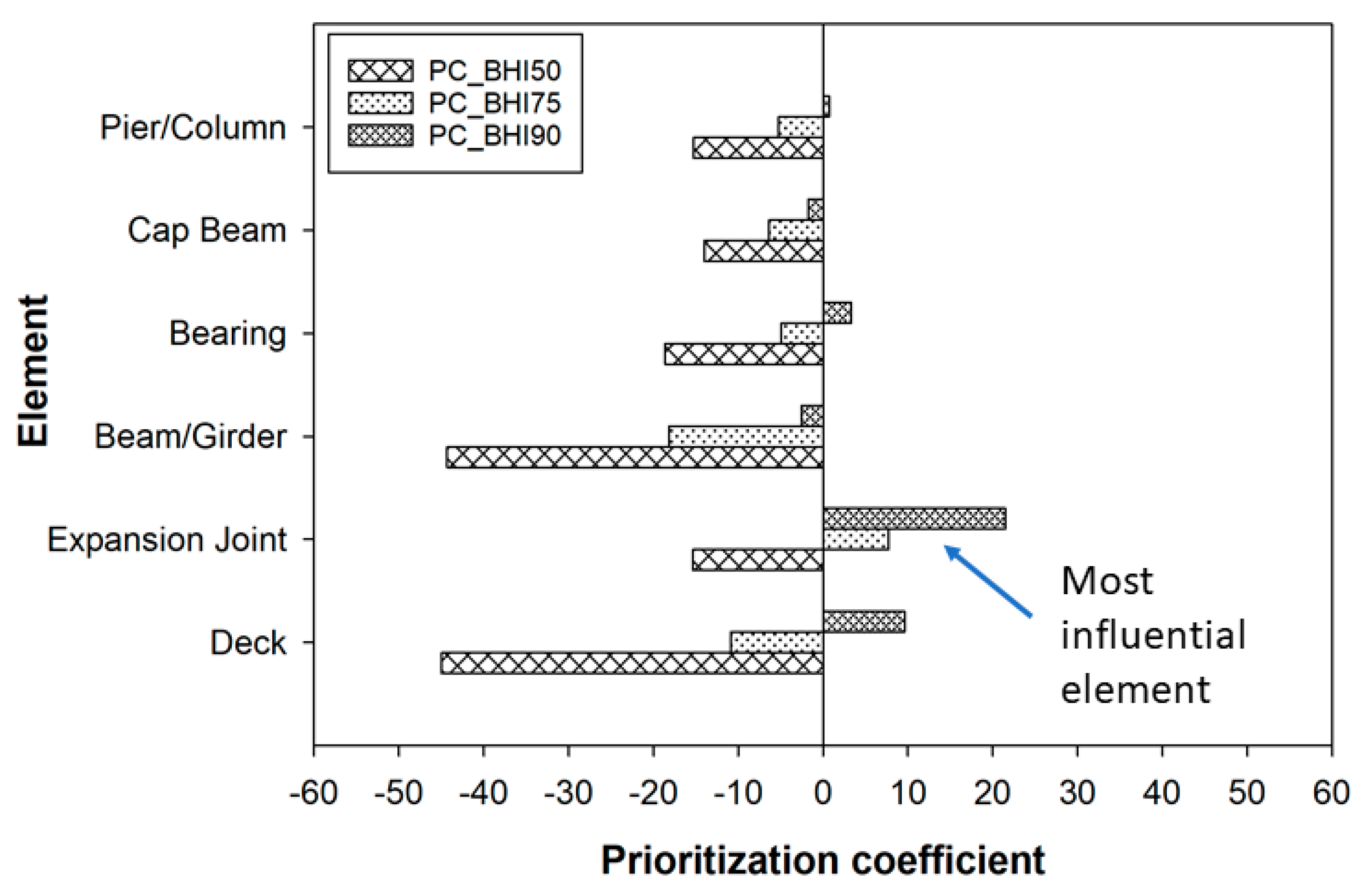
5.1. Prioritization for Bridge Maintenance

Bridge element “prioritization coefficient (PC)” is a numerical value, which defines the relative maintenance priority of Co-Active elements at discrete time. While health indexes should be time-dependent, decision making occurs at discrete times. Therefore, the proposed element ‘PC’ analysis informs state DOTs which elements are most influential for long-term bridge performance based on bridge health index depreciation models similar to one shown in Figure 13. The effective bridge preventive maintenance actions (e.g., deck treatment, beam painting, etc.) are intended to delay the need for costly rehabilitation or replacement while bridges are still in good or fair condition and before the onset of serious deterioration [44].

Thus, it is recommended that the results from the previous section are further analyzed by means of ‘PC’ defined by Equation (6). The ‘PC’ accounts for a performance target (e.g., a threshold health index) and associated performance gaps. Consequently, the ‘PC’ analysis helps prioritize preventive maintenance activities, rehabilitation, or replacement. In this equation, the subscript, ‘e’, indicates an element.

$${\mathrm{PC}}_e=[{\mathrm{HI}}_{\mathrm{e}}^{\mathrm{threshould}}·{\mathrm{HI}}_{\mathrm{e}}]\times \frac{{\mathrm{W}}_{\mathrm{e}}^{\mathrm{C}}}{100}$$

(6)

where,

• ${\mathrm{PC}}_e$ = Prioritization coefficient,
• ${\mathrm{HI}}_{\mathrm{e}}$ = Health index,
• ${\mathrm{HI}}_{\mathrm{e}}^{\mathrm{threshould}}$ = Threshold health index,
• ${\mathrm{W}}_{\mathrm{e}}^{\mathrm{C}}$ = Collaboration factor.

The prioritization coefficients (PCs) for varying BHI thresholds (50, 75, and 90) in Year 2018 are shown in Figure 14 for the case studied (prestressed concrete open girder/beam bridges) in the preceding section. Figure 15 and Figure 16 show the PCs for the other bridge groups (steel open girder/beam bridges and reinforced concrete open girder/beam with pile foundation bridges) previously identified in this paper.

When ‘PC’ is negative, it means that the element meets the performance level, having a specific prioritization requirement (see

Table 8. Prioritization coefficients (PC) scales.

Negative (-) PC		Positive (+) PC
Coefficient	Description	Coefficient	Description
PC ≥ 100	Very Low Priority	PC ≥ 100	Very High Priority
90 ≤ PC < 100	Low Priority	90 ≤ PC < 100	High Priority
80 ≤ PC < 90		80 ≤ PC < 90
70 ≤ PC < 80		70 ≤ PC < 80
60 ≤ PC < 70		60 ≤ PC < 70
50 ≤ PC < 60	Medium Priority	50 ≤ PC < 60	Medium Priority
40 ≤ PC < 50		40 ≤ PC < 50
30 ≤ PC < 40	High Priority	30 ≤ PC < 40	Low Priority
20 ≤ PC < 30		20 ≤ PC < 30
10 ≤ PC < 20		10 ≤ PC < 20
0 ≤ PC < 10	Very High Priority	0 ≤ PC < 10	Very Low Priority

). As the ‘PC’ approaches zero, elements may require preventive maintenance activities. When ‘PC’ is positive, the first part of Equation (6) represents a “performance gap” in an element. The second part, including the weighed element collaboration factors, accounts for how Co-Active elements work together to affect the overall bridge performance. When the ‘PC’ is positive and higher in value, elements are prioritized because the performance gap is larger, and the collaboration factor is higher. The higher the positive value of an element’s ‘PC’, the more influential it is in closing the “performance gap” and in meeting the agency’s performance target. However, if the agency’s benchmark HI target is lower (or 50), all elements’ condition would need a minimum improvement although elements with less negative ‘PC’ will be prioritized.

For example, in Figure 14, when the threshold BHI was 75, the ‘PC’ for expansion joint was 8, which was the highest ‘PC’, and it was the only positive ‘PC’. The pier/column’s ‘PC’ was negative but approached zero. This indicates this element would soon need attention. By comparison, the ‘PCs’ of beam/girder, bearing and cap beam in ‘PC109’ group (Figure 14) show that these elements were less critical than similar elements in ‘SO107’ group (Figure 15). Furthermore, due to the relatively lower magnitude of negative ‘PCs’, when the threshold BHI was 50, most elements in the ‘RC110’ group (Figure 16) would become critical, sooner than similar elements in the other groups.

5.2. Discussion of Results

The return on the investment (ROI) in terms of bridge service life extension is optimized when an element with the highest prioritization coefficient is replaced or repaired. This Co-Active approach and associated long-term ROI is not currently being considered by transportation agencies. Among the group of six Co-Active elements analyzed, the prioritization coefficient of the expansion joint appears to be the highest. This shows that the deterioration of expansion joints in Georgia bridges is most influential on the performance of the adjacent and underlying elements, for the group of bridges studied. The prioritization coefficient is a resourceful parameter for closing performance gaps and prioritizing elements for preventive maintenance activities, rehabilitation, or replacement.

For the three study bridge groups (steel open girder/beam bridge (SO107), prestressed concrete open girder/beam bridge (PC109), and reinforced concrete open girder/beam with pile foundation bridge (RC110), it was concluded that the expansion joint was the most influential element for improving the overall BHI, when the threshold BHI target of 75 was used. This means that by investing on expansion joint replacements in Year 20, for the prestressed concrete open girder/beam bridge (PC109) group, which contained 1439 in-service bridges in Georgia, the overall BHI would improve by 20% over the subsequent 20 years. The results from the prioritization analysis also suggest that expansion joints were the most critical element when a threshold BHI of 75 was considered.

In addition to the expansion joint and deck, the third most influential element was bearing, in the steel open girder/beam bridge (SO107), and pile, in the reinforced concrete open girder/beam with pile foundation bridge (RC110). Although cap beam element met the performance level in all the three bridge groups. Yet, the element’s PCs were not the same for the three studied groups. The relative difference in the element’s PCs, among the three study groups, had great potential for influencing the decision making process on the element’s MRR. As per the element’s MRR requirements, cap beam was more critical in reinforced concrete open girder/beam with the pile foundation bridge (RC110) group than in the steel open girder/beam bridge (SO107) and prestressed concrete open girder/beam bridge (PC109) groups. This means that the cap beam element would require MRR sooner in reinforced concrete open girder/beam with pile foundation bridge group (which contained bridges that were evenly distributed around the southern part of Georgia) than in the other two bridge groups, having a cluster of bridges around Atlanta (see inspection areas 7, 9, and 12 in Figure 3).

6. Conclusions

In this study, “Co-Active” bridge elements that act together to improve the overall bridge health index (BHI) were defined. The main advantage of using a “Co-Active” model lies in the fact that transportation agencies will be able to assess which element’s preventive maintenance, rehabilitation, or replacement (MRR) optimizes a return on investment (ROI), in terms of bridge service life. Optimization of the ROI was achieved when the Co-Active element with the highest prioritization coefficient was selected for MRR.

It was concluded that long-term gains from bridge investments (preventive maintenance, rehabilitation, or replacement) became apparent when the “Co-Active” elements were identified to extend service life of bridges. The “Co-Active” elements extended the service life of bridges through complex systems of interaction, which is a function of key parameters that define elements’ inter-dependent relationships over time. This study shows how to determine “Co-Active” coefficients and factors that enhance bridge performance by means of analyzing contingency tables. The “Co-active” model proposed in this study determines the effects of “Co-Active” elements on the bridge performance over its life cycle.

In addition to the proposed “Co-Active” model, a prioritization coefficient (PC) was introduced to account for a performance target and identify performance gaps established by a transportation agency. The proposed PC effectively found most influential MRR items in closing the performance gaps that might be present in a bridge inventory.

7. Future Work

When additional groups of “Co-Active” elements are identified, the positive outcome will amplify returns on bridge management investments. The inter-dependent relationships among “Co-Active” elements define how performance of one element affects the other bridge elements. Bridge asset managers should be able to optimize a return on investment (ROI), with respect to bridge actions (i.e., preventive maintenance, rehabilitation, or replacement), by understanding and defining inter-dependent relationships among elements. The “Co-Active” coefficients, which define the relationships among elements, vary from 0.28 to 0.99. Future research should therefore focus on identifying additional groups of Co-Active elements and improving “Co-Activeness” of elements.

References

1. AASHTO. Manual for Bridge Element Inspection, 2nd ed.; American Association of State Highway and Transportation Officials: Washington, DC, USA, 2019. [Google Scholar]
2. Phillips, P.S.T. Predicting Costs for Bridge Replacement Projects; The University of North Carolina at Charlotte: Charlotte, NC, USA, 2017. [Google Scholar]
3. Puls, E.; Hueste, M.B.D.; Hurlebaus, S.; Damnjanovic, I. Prioritization of a bridge inventory for historic preservation: A case study for Tarrant County, Texas. Publ. Works Manag. Pol. 2018, 23, 205–220. [Google Scholar] [CrossRef]
4. Sabatino, S.; Frangopol, D.M. Decision support system for optimum lifetime sustainability-based maintenance planning of highway bridges. In Proceedings of the International Conference on Sustainable Infrastructure, New York, NY, USA, 26–28 October 2017. [Google Scholar]
5. Inkoom, S.; Sobanjo, J. Availability function as bridge element’s importance weight in computing overall bridge health index. Struct. Infrastruct. Eng. 2018, 14, 1–13. [Google Scholar] [CrossRef]
6. Jiang, X.; Rens, K.L. Bridge health index for the city and county of Denver, Colorado. I: Current methodology. J. Perform. Constr. Facil. 2010, 24, 580–587. [Google Scholar] [CrossRef]
7. Jiang, X.; Rens, K.L. Bridge health index for the city and county of Denver, Colorado. II: Denver bridge health index. J. Perform. Constr. Facil. 2010, 24, 588–596. [Google Scholar] [CrossRef]
8. Inkoom, S.; Sobanjo, J.O.; Thompson, P.D.; Kerr, R.; Twumasi-Boakye, R. Bridge health index: study of element condition states and importance weights. Transport. Res. Rec. 2017, 2612, 67–75. [Google Scholar] [CrossRef]
9. Adhikari, R.S.; Moselhi, O.; Bagchi, A. A study of image-based element condition index for bridge inspection. In Proceedings of the International Symposium on Automation and Robotics in Construction, Montréal, QC, Canada, 11–15 August 2013. [Google Scholar]
10. Sobanjo, J.O.; Thompson, P.D. Implementation of the 2013 AASHTO manual for bridge element inspection; Report No. BDV30-977-07; Florida State University: Tallahassee, FL, USA, 2016; p. 179. [Google Scholar]
11. Anderson, I.; Rizzo, D.M.; Huston, D.R.; Dewoolkar, M.M. Analysis of bridge and stream conditions of over 300 Vermont bridges damaged in Tropical Storm Irene. Struct. Infrastruct. Eng. 2017, 13, 1437–1450. [Google Scholar] [CrossRef]
12. Weidner, J.; Prader, J.; Dubbs, N.; Moon, F.; Aktan, A.E.; Taylor, J.; Skeens, C. Extending the life of aged, reinforced concrete arch bridges through load testing and monitoring. ACI Spec. Publ. 2018, 323, 12.11–12.16. [Google Scholar]
13. Chase, S.B.; Adu-Gyamfi, Y.; Aktan, A.; Minaie, E. Synthesis of National and International Methodologies Used for Bridge Health Indices; FHWA-HRT-15-081; Federal Highway Administration: McLean, VA, USA, 2016.
14. Lake, N.; Seskis, J. Bridge Management Using Performance Models; AP-T258/13; Austroads: New South Wales, Australia, 2013. [Google Scholar]
15. Jonnalagadda, S.; Ross, B.E.; Khademi, A. A modelling approach for evaluating the effects of design variables on bridge condition ratings. J. Struct. Integrity Maint. 2016, 1, 167–176. [Google Scholar] [CrossRef]
16. Fereshtehnejad, E.; Hur, J.; Shafieezadeh, A.; Brokaw, M.; Backs, J.; Noll, B.; Waheed, A. A bridge performance index with objective incorporation of safety risks. In Proceedings of the Transportation Research Board 97th Annual Meeting, Washington, DC, USA, 7–11 January 2018. [Google Scholar]
17. Jeong, Y.; Kim, W.; Lee, I.; Lee, J. Bridge inspection practices and bridge management programs in China, Japan, Korea, and US. J. Struct. Integrity Maint. 2018, 3, 126–135. [Google Scholar] [CrossRef]
18. Verhoeven, J.; Flintsch, G. Generalized framework for developing a corridor-level infrastructure health index. Transport. Res. Rec. 2011, 20–27. [Google Scholar] [CrossRef]
19. Matteo, A.; Milton, J.; Springer, T. Using Asset Valuation as a Basis for Bridge Maintenance and Replacement Decisions. Available online: http://onlinepubs.trb.org/Onlinepubs/webinars/160411.pdf (accessed on 18 September 2017).
20. Matteo, A. State of Good Reapir (SGR) Program: Bridge Prioritization Formula. Available online: http://www.virginiadot.org/business/resources/local_assistance/StateofGoodRepair/SGR_Locally_Owned_Bridges_Prioritization_Process_-_Adam_Matteo_PowerPoint.pdf (accessed on 15 January 2020).
21. Shepard, R.W.; Johnson, M.B. California Bridge Health Index: A Diagnostic Tool to Maximize Bridge Longevity, Investment; Transportation Research Board: Washington, DC, USA, 2001; pp. 6–11. [Google Scholar]
22. Spyrakos, C.; Loannidis, G. Seismic behavior of a post-tensioned integral bridge including soil–structure interaction (SSI). Soil Dyn. Earthq. Eng. 2003, 23, 53–63. [Google Scholar] [CrossRef]
23. Mehrabi, A.B. In-service evaluation of cable-stayed bridges, overview of available methods and findings. J. Bridge Eng. 2006, 11, 716–724. [Google Scholar] [CrossRef]
24. Enright, M.P.; Frangopol, D.M. Survey and evaluation of damaged concrete bridges. J. Bridge Eng. 2000, 5, 31–38. [Google Scholar] [CrossRef]
25. Yianni, P.C.; Rama, D.; Neves, L.C.; Andrews, J.D.; Castlo, D. A Petri-Net-based modelling approach to railway bridge asset management. Struct. Infrastruct. Eng. 2017, 13, 287–297. [Google Scholar] [CrossRef] [Green Version]
26. Yarnold, M.; Weidner, J. Monitoring of a bascule bridge during construction. In Proceedings of the Transportation Research Board 95th Annual Meeting, Washington, DC, USA, 10–14 January 2016. [Google Scholar]
27. De Risi, R.; Di Sarno, L.; Paolacci, F. Probabilistic seismic performance assessment of an existing RC bridge with portal-frame piers designed for gravity loads only. Eng. Struct. 2017, 145, 348–367. [Google Scholar] [CrossRef]
28. Thompson, P.D.; Bye, P.; Western, J.; Valeo, M. Risk assessment for bridge management systems. In Proceedings of the 9th International Conference on Bridge Maintenance, Safety and Management, Melbourne, Australia, 9–13 July 2018. [Google Scholar]
29. Thomas, O.; Sobanjo, J. Semi-Markov models for the deterioration of bridge elements. J. Infrastruct. Syst. 2016, 22, 04016010. [Google Scholar] [CrossRef]
30. Thomas, O.; Sobanjo, J. Comparison of Markov chain and semi-Markov models for crack deterioration on flexible pavements. J. Infrastruct. Syst. 2012, 19, 186–195. [Google Scholar] [CrossRef]
31. Salim, W.S.W.; Liew, M.S.; Shafie, A.f. Qualitative fault tree and event tree model of bridge defect for reinforced concrete highway bridge. In Proceedings of the International Civil and Infrastructure Engineering Conference Kota Kinabalu, Sabah, Malaysia, 28 September–1 October 2014; pp. 639–650. [Google Scholar]
32. Patidar, V.; Labi, S.; Sinha, K.; Thompson, P. Multi-Objective Optimization for Bridge Management Systems; Report No. 590; Transportation Research Board: Washington, DC, USA, 2007. [Google Scholar]
33. Hearn, G. Element-Level Performance Measures for Bridge Preservation; Transportation Research Board: Washington, DC, USA, 2015; pp. 10–17. [Google Scholar]
34. Kosgodagan-Dalla Torre, A.; Yeung, T.G.; Morales-Nápoles, O.; Castanier, B.; Maljaars, J.; Courage, W. A two-dimension dynamic Bayesian network for large-scale degradation modeling with an application to a bridges network. Comput-Aided Civ. Infrastruct. Eng. 2017, 32, 641–656. [Google Scholar] [CrossRef] [Green Version]
35. Dori, G.; Wild, M.; Borrmann, A.; Fischer, O. A system model based approach for lifecycle monitoring of bridges. In Proceedings of the 3rd International Conference on Soft Computing Technology in Civil, Structural and Environmental Engineering, Cagliari, Sardinia, Italy, 3–6 September 2013. [Google Scholar]
36. LeBeau, K.; Wadia-Fascetti, S. A fault tree model of bridge deterioration. In Proceedings of the 8th ASCE Specialty Conference on Probabilistic Mechanics and Structural Reliability, Notre Dame, IN, USA, 24–26 July 2000. [Google Scholar]
37. Sianipar, P.R.; Adams, T.M. Fault-tree model of bridge element deterioration due to interaction. J. Infrastruct. Syst. 1997, 3, 103–110. [Google Scholar] [CrossRef]
38. NCHRP. Performance measures and targets for transportation asset management; 551; Transportation Research Board: Washington, DC, USA, 2006. [Google Scholar]
39. Bu, G.; Lee, J.; Guan, H.; Blumenstein, M.; Loo, Y.-C. Improving reliability of Markov-based bridge deterioration model using Artificial Neural Network. In Proceedings of the IABSE-IASS Symposium - Taller, Longer, Lighter, London, UK, 20–23 September 2011. [Google Scholar]
40. Chang, M.; Maguire, M. Developing Deterioration Models for Wyoming Bridges; FHWA-WY-16/09F; Utah State University: Logan, UT, USA, 2016. [Google Scholar]
41. Chorzepa, M.G.; Durham, S.; Kim, S.K.; Oyegbile, O.B. Bridge Asset Valuation Utilizing Condition States Obtained from Element-Based Inspection Inventories and Depreciation Models over the Life Cycle of the Assets; Report No. FHWA-GA-19-1728; University of Georgia: Atlanta, GA, USA, 2019; p. 101. [Google Scholar]
42. Embrechts, P.; McNeil, A.J.; Straumann, D. Correlation and dependence in risk management: properties and pitfalls. In Risk Management: Value at Risk and Beyond; Cambridge University Press: Cambridge, UK, 2002; Volume 1, pp. 176–223. [Google Scholar]
43. Agrawal, A.K.; Kawaguchi, A.; Chen, Z. Deterioration rates of typical bridge elements in New York. J. Bridge Eng. 2010, 15, 419–429. [Google Scholar] [CrossRef]
44. FHWA. Bridge Preservation Guide: Maintaining a Resilient Infrastructure to Preserve Mobility; FHWA-HIF-18-022; Federal Highway Administration: Washington, DC, USA, 2018.
Figure 1. Bridge and element counts in the Georgia (GA) bridge inventory. (a) The number of bridges constructed in 12 age bins. (b) The number of elements in a bridge by year constructed.
Infrastructures 05 00013 g001
Figure 2. Typical bridge in the ‘PC109’ group.
Infrastructures 05 00013 g002
Figure 3. Geographical locations of the identified bridge groups (SO107, PC109, and RC110) in twelve (12) inspection areas in Georgia. Notes: SO107 = Steel open girder/beam bridge; PC109 = Prestressed concrete girder/beam bridges; RC110 = Reinforced concrete open girder/beam bridge.
Infrastructures 05 00013 g003
Figure 4. Multilinear function to aggregate element percentage quantities (age bin 1940).
Infrastructures 05 00013 g004
Figure 5. Flowchart showing how one element’s HI change affects a time-history of other elements.
Infrastructures 05 00013 g005
Figure 6. Contingency table for the Co-Active elements in the ‘SO107’ group. Notes: * = Co-Active coefficient corresponding to “Row 1”, “Col. 4”.
Infrastructures 05 00013 g006
Figure 7. Contingency table for the Co-Active elements in the ‘PC109’ group.
Infrastructures 05 00013 g007
Figure 8. Contingency table for the Co-Active elements in the ‘RC110’ group.
Infrastructures 05 00013 g008
Figure 9. A two-span bridge with a group of Co-Active elements in the group PC109.
Infrastructures 05 00013 g009
Figure 10. Dominant inter-dependencies among the Co-Active elements in the group PC109.
Infrastructures 05 00013 g010
Figure 11. Bridge overall and element health index prediction models (group PC109).
Infrastructures 05 00013 g011
Figure 12. Effect of an Expansion Joint No. 301 Replacement (before applying the Co-Active approach).
Infrastructures 05 00013 g012
Figure 13. Effect of an Expansion Joint No. 301 Replacement (after applying the Co-Active approach).
Infrastructures 05 00013 g013
Figure 14. Prioritization coefficients in the ‘PC109’ group for Bridge Health Index (BHI) thresholds (50, 75, and 90). Notes: negative value of ‘PC’ = the element meets the performance level; positive value of ‘PC’ = the element does not meet the performance level.
Infrastructures 05 00013 g014
Figure 15. Prioritization coefficients in the ‘SO107’ group for BHI thresholds (50, 75, and 90).
Infrastructures 05 00013 g015
Figure 16. Prioritization coefficients in the ‘RC110’ group for BHI thresholds (50, 75, and 90).
Infrastructures 05 00013 g016