Generation Units Maintenance in Combined Heat and Power Integrated Systems Using the Mixed Integer Quadratic Programming Approach

Abstract

Yearly generation maintenance scheduling (GMS) of generation units is important in each system such as combined heat and power (CHP)-based systems to decrease sudden failures and premature degradation of units. Imposing repair costs and reliability deterioration of system are the consequences of ignoring the GMS program. In this regard, this research accomplishes GMS inside CHP-based systems in order to determine the optimal intervals for predetermined maintenance required duration of CHPs and other units. In this paper, cost minimization is targeted, and violation of units’ technical constraints like feasible operation region of CHPs and power/heat demand balances are avoided by considering related constraints. Demand-response-based short-term generation scheduling is accomplished in this paper considering the maintenance intervals obtained in the long-term plan. Numerical simulation is performed and discussed in detail to evaluate the application of the suggested mixed-integer quadratic programming model that implemented in the General Algebraic Modeling System software package for optimization. Numerical simulation is performed to justify the model effectiveness. The results reveal that long-term maintenance scheduling considerably impacts short-term generation scheduling and total operation cost. Additionally, it is found that the demand response is effective from the cost perspective and changes the generation schedule.

1. Introduction

Combined heat and power (CHP) generation units have high efficiency for simultaneous generation of electricity and heat compared to conventional generators such as power-only generators and heat-only boilers Salgado and Pedrero [1]. Although a CHP unit supplies the power and heat demands efficiently, continuous operation of this element in a long-term horizon without periodic maintenance leads to enhanced probability of unexpected failures. Additionally, premature degradation is unavoidable for CHP and other units in the case of ignoring yearly maintenance. If the units are randomly under maintenance in typical weeks, the system reliability may deteriorate, resulting from a lack of reserve, and even deterioration in system stability arising from the simultaneous maintenance of units. Furthermore, ignoring maintenance services imposes additional costs for repairing the generation units, which have faced sudden failures.

The generation maintenance scheduling (GMS) program is the solution of the proposed issue and is used by researchers to handle the mentioned challenge by taking into account the duration of the maintenance required of each unit for the coordination of maintenance scheduling. This program can optimally schedule the planned outage of existence units in CHP-integrated systems with simultaneous optimization of the maintenance intervals for all existence generation units.

In addition to GMS, demand response programs can also impact the short-term generation scheduling of CHP-based systems. Demand response is one of the methods used to enhance power system flexibility Mirzaei et al. [2] and is mainly adopted for cost reduction Sadeghian et al. [3] and reliability improvement Sadeghian et al. [4]. A shift-based demand response model has been adopted by researchers for economic dispatch of CHP-based microgrids Nazari-Heris et al. [5]. In Ahmadi and Rezaei [6], a step-wise demand response program based on demand reduction has been used for cost improvement in isolated microgrids. In reference Rafinia et al. [7], demand response resources are considered in the load shedding program. In another attempt Majidi et al. [8], demand response is used for improving the cost and emission of energy hub systems. Furthermore, in references Oshnoei and Khezri et al. [9,10], researchers have used demand response for the frequency control of a power system. In the current research, a shift-based demand response program has been used for cost reduction.

In the following paragraphs, first, the studies related to generation scheduling in CHP-based systems are reviewed. Afterwards, the previous studies related to GMS optimization problem are discussed, none of which has considered the CHP-based systems.

Optimal generation scheduling in CHP-integrated systems has been widely investigated in the literature. A literature review on the optimal scheduling of CHP units economic dispatch by heuristic algorithms from an economic and environmental point of views is accomplished in Nazari-heris et al. [11]. The authors in Mohammadi-Ivatloo et al. [12] have solved the cost-based CHP economic dispatch problem using the particle swarm optimization algorithm, in which the acceleration coefficients are changed respect to the iterations to improve the application of the algorithm. In another study, the CHP units economic dispatch problem using the real coded genetic algorithm is studied Haghrah et al. [13]. This research has adapted the improved Mühlenbein mutation to speed up the algorithm in solving the resulted problem. In Zou et al. [14], an improved genetic algorithm is employed to solve the economic dispatch problem in CHP-based systems. A cost-based economic dispatch problem in large-scale CHP-based systems is introduced in Nazari-heris et al. [15]. Some researchers have presented linearization techniques to change the mixed-integer non-linear programming model into more simple models for the day-ahead stochastic scheduling of CHP integrated systems aims to minimizing the total cost Kia et al. [16]. Researchers have also investigated the generation scheduling of heat and power based microgrids in the presence of renewable energy sources in Mazidi et al. [17]. In some research Lyu and Zhang et al. [18,19], flexible CHP units with energy storage systems are adopted to meet the intermittence nature of renewable energy sources. In Yuan et al. [20], economic dispatch of CHP units is performed in the presence of electrical and thermal energy storage. Furthermore, in Merkert et al. [21], a unit commitment model is presented for optimal operation of CHP units considering the thermal inertia of connected district heating grid. Researchers in references Li and Wang et al. [22,23] have investigated an environmental cost-based model for economic dispatch of CHP units. In another attempt Dinh et al. [24], a modified bat algorithm is employed for economic dispatch of CHP units. Optimal operation of CHP units for real cases has been investigated in references Amber and Waqar et al. [25,26]. Although the optimal generation of CHP-based systems have been investigated by researchers, the maintenance scheduling of generation units in a CHP-based system has not been investigated so far.

The GMS problem in different environments and systems has been investigated in the literature. Researchers have investigated risk-constrained stochastic GMS problem in virtual power plants Sadeghian et al. [3]. In Conejo et al. [27], the authors studied the maintenance scheduling in restructured power systems. In another study, the maintenance management of generation units in oligopolistic electricity markets is presented Sadeghian et al. [28]. The maintenance scheduling in deregulated electricity markets has been developed in Dahal et al. [29]. The GMS problem for hydro-power generators is investigated in literature Rodriguez et al. [30]. In another attempt, GMS optimization is accomplished in smart distribution systems Fotouhi Ghazvini et al. [31]. A comprehensive review on maintenance scheduling in power systems is accomplished in Froger et al. [32]. Various methods are employed in the literature for optimizing the GMS problem [33,34,35,36,37]. The authors in Eygelaar et al. [33] have developed a risk-constrained GMS criterion based on unexpected failures of generation units. Optimal generation and maintenance management adopting the discrete integer cuckoo search optimization algorithm is investigated in Lakshminarayanan and Kaur [34] in order to maximize and distribute the reserve power across the weeks of the year evenly. Moreover, in Parhizkar et al. [35], a methodology for co-scheduling of generation and maintenance considering the aging of power plants in long-term with the aim of maximizing the total profit is introduced. In Wang et al. [36], the authors have suggested reliability-based maintenance scheduling of generation units using an MIP model. Furthermore, in Balaji et al. [37], the GMS with the objective of operation cost minimization is investigated, in which the differential evolution algorithm is used to optimize the model. Although the above-mentioned papers have studied GMS optimization, maintenance scheduling in a CHP-based system has not been investigated.

Based on the literature review of GMS as well as literature review of CHP-based systems, it is observed that GMS in CHP-based systems has not been studied so far. In the other words, although the GMS problem has been widely investigated in the literature, the GMS problem has not been investigated in CHP-based systems until now. In this paper, the GMS program in CHP-integrated systems is accomplished and aims at cost minimization. Short-term generation scheduling is also performed considering the yearly maintenance schedule that is obtained in the long-term plan. Demand response is also considered in the model to evaluate the maintenance schedule and cost results in the presence of load response. The resulted problem is formulated as a mixed integer quadratic programming (MIQP) model and implemented in the general algebraic modelling system (GAMS) package software. Related operational and security constraints such as feasible operation region (FOR) of CHP units is taken into account. Numerical results are adapted and discussed to verify the effectiveness of the proposed model.

The paper is structured as follows: the problem formulation related to GMS in a CHP-based system is explained in Section 2. Section 3 presents the numerical simulation to justify the effectiveness of the offered model for GMS in CHP-based systems. Finally, the paper is concluded in Section 4.

2. Problem Formulation

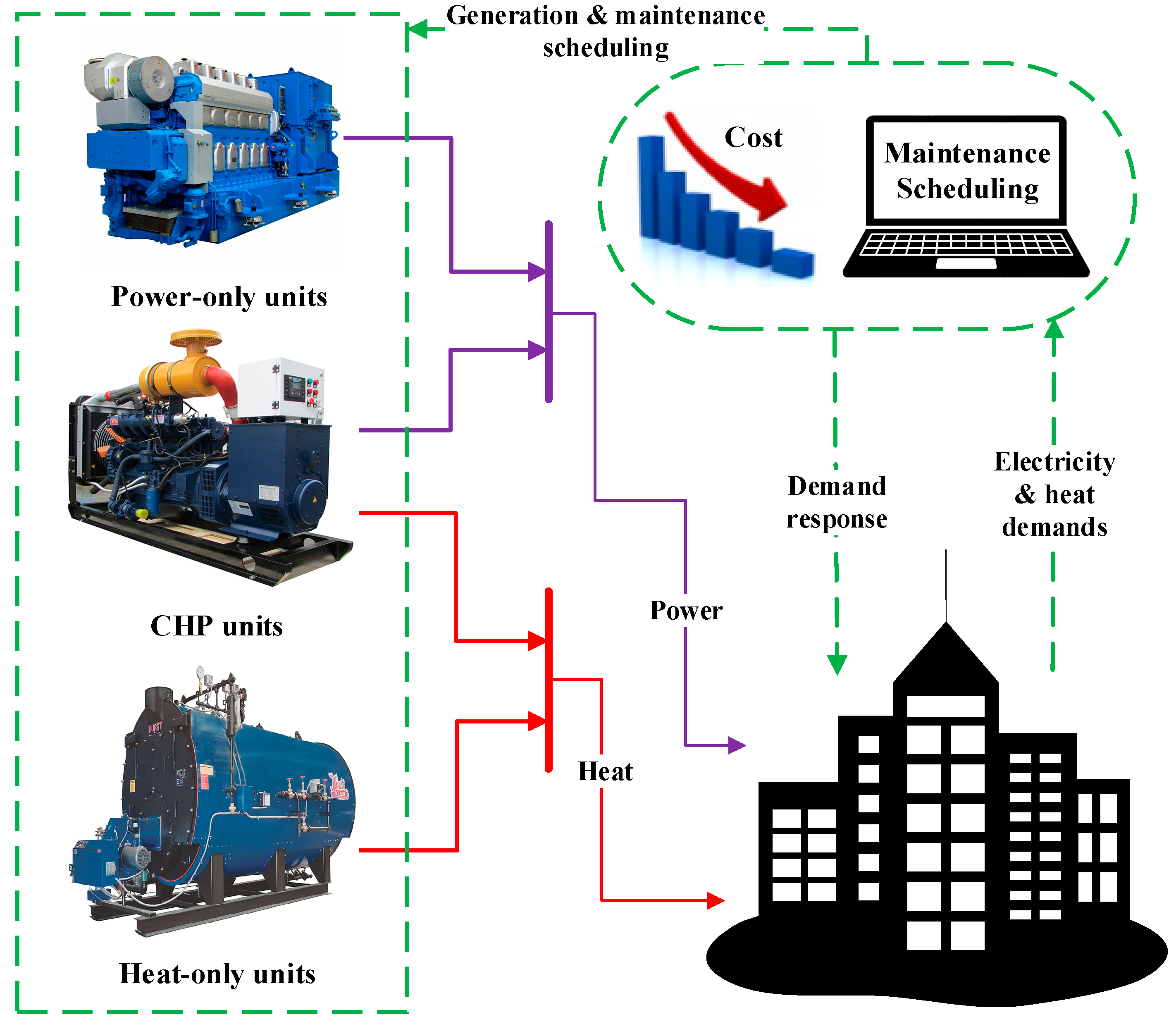
A diagram of the CHP-based system and its elements for preventive GMS is depicted in Figure 1. The network power and heat demands can be predicted by different methods, such as principal component analysis Moradzadeh and Garcia Marquez et al. [38,39], neural networks Moradzadeh et al. [40], deep learning Moradzadeh and Pourhossein [41], support vector machines Moradzadeh and Pourhossein [42], or other methods Moradzadeh and Khaffafi [43], and supplied by CHP units and the other units, including power-only and heat-only units. The electricity demand is supplied by power-only and CHP units, while the heat demand is supplied by heat-only and CHP units. CHP units can supply both the power and heat demands simultaneously, and while they can be the only source of power, they cannot be the sole heat source. In order to accomplish maintenance management, the system operator considers the maintenance required durations of all units in a unit problem for coordinating the planned outage. The maintenance intervals are determined through a long-term plan Marquez [44]. Afterward, in short-term generation scheduling, the units that are under yearly maintenance do not participate in power generation. The operator optimizes the maintenance schedule and announces it to the units for implementation. In short-term horizons, GMS decreases the units’ failure, which results in lower repair cost and higher system reliability and stability Chacon Munoz et al. [45]. Additionally, in long-term horizons, GMS delays the degradation of units, which results in a delay in the need for constructing new power plants.

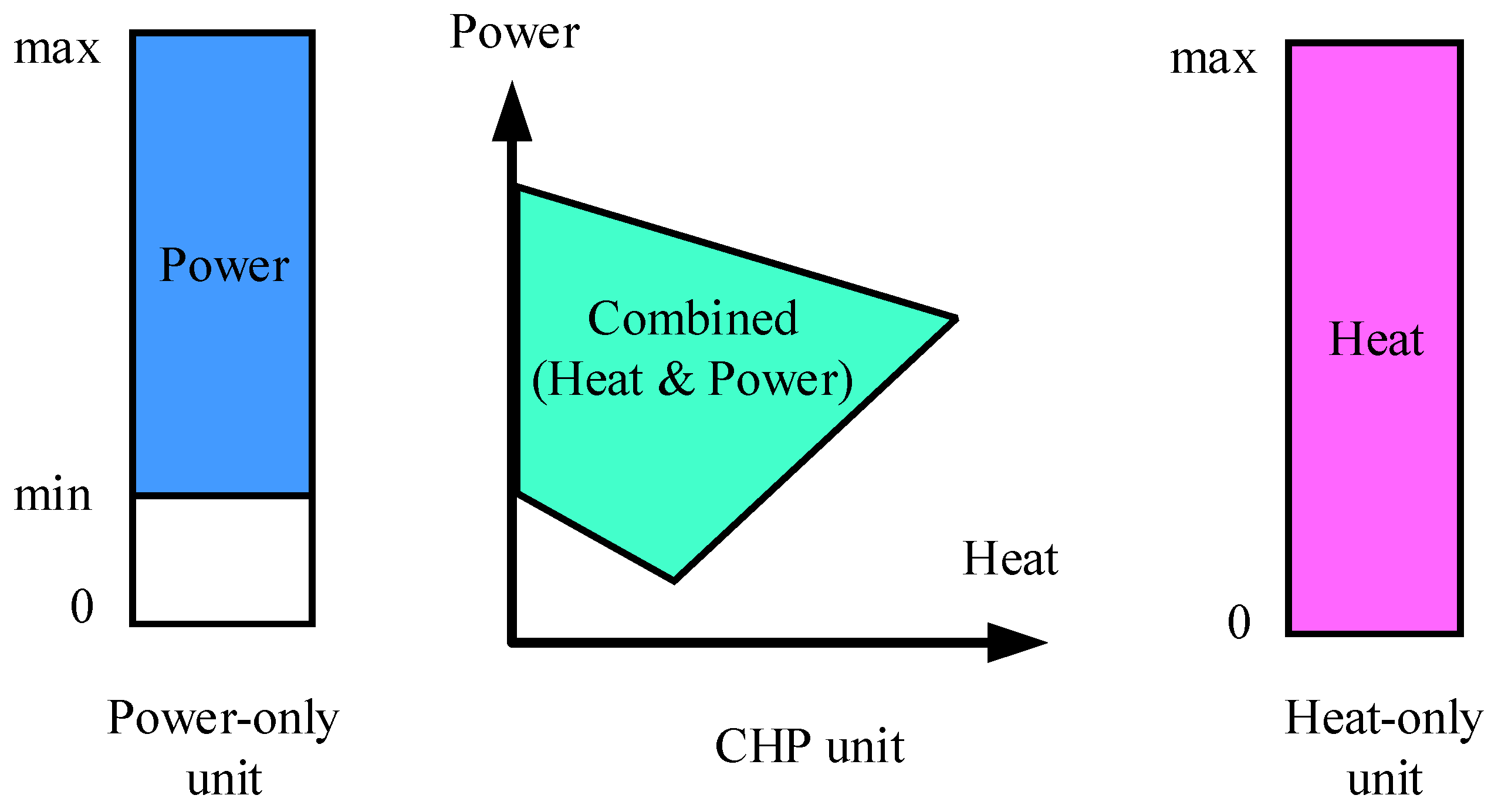
The feasible region of the CHP and the other units is illustrated in Figure 2. Their different functions in the generation of power/heat for load supply is observed in this figure. As seen, the feasible regions of the units are not similar. The feasible region of the power-only unit has a minimum and a maximum value, while the heat-only unit has a value between zero and a maximum value. On the other hand, the feasible region of CHP is considerably different with the feasible region of the two other units, which complicates the optimization of the problem.

The objective function in this research is the overall cost of the CHP-integrated system using Equation (1). The first, second, and third terms show the cost of power-only, CHP, and heat-only units, respectively. The units’ costs consist of the polynomial cost function and the maintenance cost. It is worth mentioning that for the long-term plan (for maintenance scheduling), the time horizon is 52 weeks, and hence, the range of t is (1, 52), while in the short-term plan (for generation scheduling), the time horizon is 24 h and hence, the range of t is (1, 24). Additionally, the time accuracy ($T_A$) is $7\times 24$ h and 1 h, respectively, for the long-term and short-term plans. All the symbols have been specified in the nomenclature.

$$TC={\displaystyle \sum _t{T}_A\left\{\begin{array}{l}\left({\alpha }^i{(P_P^{i,t})}^2+{\beta }^i{P}_P^{i,t}+{\gamma }^i+M{C}_P^i{x}_P^{i,t}{P}_P^{Max,i}\right)\\ +\left(\begin{array}{l}{a}^j{(P_{CHP}^{j,t})}^2+b^j{P}_{CHP}^{j,t}+c^j\\ +d^j{(H_{CHP}^{j,t})}^2+e^j{H}_{CHP}^{j,t}+f^j{H}_{CHP}^{j,t}{P}_{CHP}^{j,t}\\ +M{C}_{CHP}^j{x}_{CHP}^{j,t}{P}_{CHP}^{Max,j}\end{array}\right)\\ +\left({\tau }^k{(H_H^{k,t})}^2+{\mu }^k{H}_H^{k,t}+{\sigma }^k+M{C}_H^k{x}_H^{k,t}{P}_H^{Max,k}\right)\end{array}\right\}}$$

(1)

The maintenance variables in the proposed optimization model is determined by x binary variable in which 1 shows the maintenance state and 0 represents the normal operation of units. It is clear that when a unit is under maintenance, it does not contribute to demand supply. This variable is only used in the long-term plan. In the short-term plan, when a unit is under maintenance (obtained by the long-term plan), the variable x is fixed to 1.

The power and heat generated by power-only and heat-only units are limited as Equations (2) and (3), respectively.

$$P_{P,min}^i{s}_P^{i,t}<P_P^{i,t}<P_{P,max}^i{s}_P^{i,t}$$

(2)

$$H_{H,min}^k{s}_H^{k,t}<H_H^{k,t}<H_{H,max}^k{s}_H^{k,t}$$

(3)

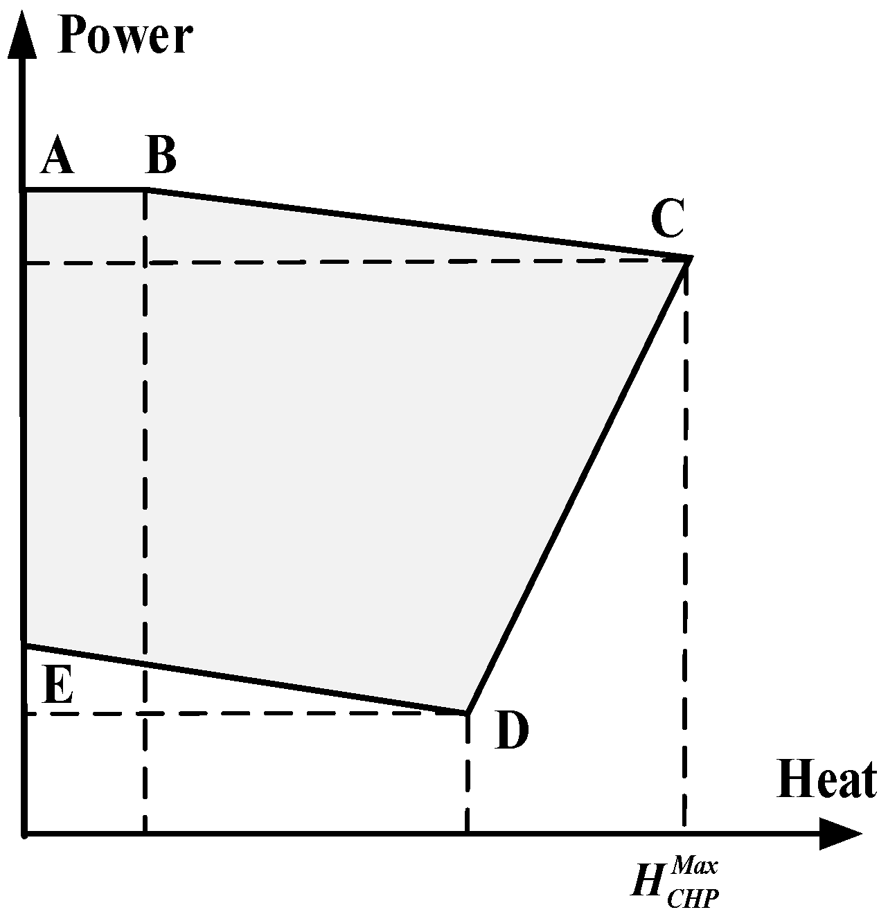
For the limitation of power and heat generated by CHP units, the parametric feasible operation region (FOR) of Figure 3 is considered. This figure is a detailed FOR of the typical CHP presented in Figure 2 to form the FOR constraints. It demonstrates that the power and heat generated by a CHP unit are related to each other. As mentioned, a CHP cannot generate heat solely, while the power can be generated solely by such units.

The heat generated by CHP units is limited as

$$H_{CHP,\max }^j{s}_{CHP}^{j,t}<H_{CHP}^{j,t}<H_{CHP,\max }^j{s}_{CHP}^{j,t}$$

(4)

To limit the power generated by CHP units, Equations (5)–(8) are used to ensure that the solutions will be in the FOR of each CHP unit. The variable $s_{CHP}^{j,t}$ in these equations is used for this aim that validates both the states of off and on, such that, in case of the on state, the FOR must be satisfied. In the other word, a CHP is off or operates in its FOR.

$$P_{CHP}^{j,t}<[\frac{P_{CHP,B}^j-P_{CHP,A}^j}{H_{CHP,B}^j-H_{CHP,A}^j}(H_{CHP}^{j,t}-H_{CHP,B}^j)+P_{CHP,B}^j]s_{CHP}^{j,t}$$

(5)

$$P_{CHP}^{j,t}<[\frac{P_{CHP,C}^j-P_{CHP,B}^j}{H_{CHP,C}^j-H_{CHP,B}^j}(H_{CHP}^{j,t}-H_{CHP,B}^j)+P_{CHP,B}^j]s_{CHP}^{j,t}$$

(6)

$$P_{CHP}^{j,t}>[\frac{P_{CHP,D}^j-P_{CHP,E}^j}{H_{CHP,D}^j-H_{CHP,E}^j}(H_{CHP}^{j,t}-H_{CHP,D}^j)+P_{CHP,D}^j]s_{CHP}^{j,t}$$

(7)

$$P_{CHP}^{j,t}>[\frac{P_{CHP,C}^j-P_{CHP,D}^j}{H_{CHP,C}^j-H_{CHP,D}^j}(H_{CHP}^{j,t}-H_{CHP,D}^j)+P_{CHP,D}^j]s_{CHP}^{j,t}$$

(8)

It is clear that the needed maintenance duration for different units is not identical. The needed maintenance duration for power-only, CHP, and heat-only units is taken into account as Sadeghian et al. [46],

$${\displaystyle \sum _t{x}_P^{i,t}=N_P^i}$$

(9)

$${\displaystyle \sum _t{x}_{CHP}^{j,t}=N_{CHP}^j}$$

(10)

$${\displaystyle \sum _t{x}_H^{k,t}=N_H^k}$$

(11)

The maintenance period of each unit must be in consecutive intervals so that the maintenance service can be completed by crews. The continuity of maintenance interval can be taken into account by,

$$x_P^{i,t}-x_P^{i,t-1}\le x_P^{i,t-1+N_P^i}$$

(12)

$$x_{CHP}^{j,t}-x_{CHP}^{j,t-1}\le x_{CHP}^{j,t-1+N_{CHP}^j}$$

(13)

$$x_H^{k,t}-x_H^{k,t-1}\le x_H^{k,t-1+N_H^k}$$

(14)

Each unit in each time interval can have only one state of maintenance (x = 1) or normal operation (s = 1). If none of them happens, the unit is off but both of them cannot be happen simultaneously. This constraint is expressed as,

$$s_P^{i,t}+x_P^{i,t}\le 1$$

(15)

$$s_{CHP}^{j,t}+x_{CHP}^{j,t}\le 1$$

(16)

$$s_H^{k,t}+x_H^{k,t}\le 1$$

(17)

In this research, the following constraints are adopted to limit the total number of simultaneous under-maintenance units as much as possible. For instance, when total number of needed weeks for maintenance of units is 53, at least one week has two under-maintenance units, and hence, the total number of simultaneous under-maintenance units in each week is lower than 2. This constraint is separately considered for power-producing units (power-only and CHP units) and heat-producing units (CHP and heat-only units) as,

$${\displaystyle \sum _i{x}_P^{i,t}}+{\displaystyle \sum _j{x}_{CHP}^{j,t}}\le \lceil \frac{1}{52}({\displaystyle \sum _i{N}_P^i}+{\displaystyle \sum _j{N}_{CHP}^j})\rceil$$

(18)

$${\displaystyle \sum _j{x}_{CHP}^{j,t}}+{\displaystyle \sum _k{x}_H^{k,t}}\le \lceil \frac{1}{52}({\displaystyle \sum _j{N}_{CHP}^j}+{\displaystyle \sum _k{N}_H^k})\rceil$$

(19)

where $\lceil \rceil$ shows the ceiling function.

Constraints regarding the power and heat balances are calculated using Equations (23) and (24), respectively. Based on Equation (20), the power-only and CHP units participate in power generation to supply the power demand. On the other hand, the CHP and heat-only units participate in heat generation to meet the heat load of the system.

$${\displaystyle \sum _i{P}_P^{i,t}}+{\displaystyle \sum _j{P}_{CHP}^{j,t}}=D_P^t$$

(20)

$${\displaystyle \sum _j{H}_{CHP}^{j,t}}+{\displaystyle \sum _k{H}_H^{k,t}}=D_H^t$$

(21)

In this research, demand response is implemented to evaluate its impact on overall cost of the system. The time of use demand response program is implemented as follows:

$$D_{P,DR}^t=D_P^t+D_{Sh}^t$$

(22)

The movable load in each period is obtained as

$$D_{Sh}^t=\frac{F_{DR}^t}{100}{D}_P^t$$

(23)

The movable load in each period is limited as

$$\left|F_{DR}^t\right|\le F_{DR,\max }$$

(24)

The following constraint illustrates that the total amount of shifted loads over a daily period is equal to zero.

$${\displaystyle \sum _t{D}_{Sh}^t}=0$$

(25)

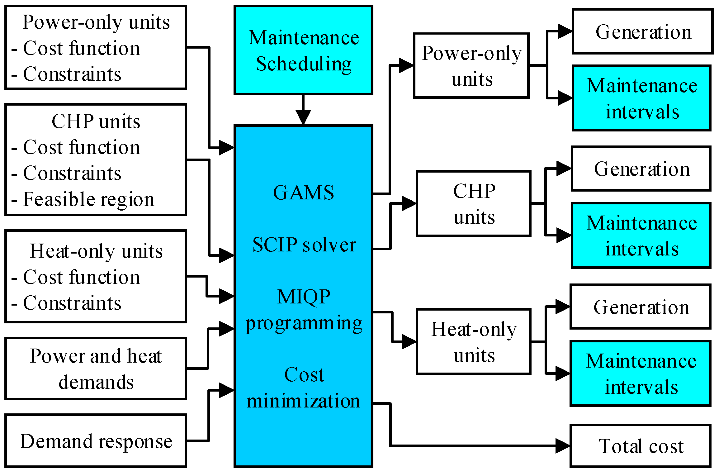
A flowchart of the suggested model for GMS in CHP-based systems is presented in Figure 4. The security and operational constraints are considered in the proposed mixed integer quadratic programming (MIQP) model Lazimy [47] for minimizing the overall cost of the system. As mentioned, MIQP stands for mixed integer quadratic programming. This optimization model stands for a model that includes both the continuous and integer variables and also has quadratic terms such as the proposed model (the objective function and its constraints). The resulted MIQP model is implemented in the GAMS software package Brooke et al. [48] version 27.3 and optimized using solving constraint integer programs (SCIP) solver Achterberg [49]. This solver performs total control of the solution process by access to the detailed information of the process. The problem is executed in a system with an Intel core i5 (Quad Core 5th Generation) @ 2.5 GHz and 6-GB of RAM.

3. Numerical Results

In this section, numerical simulation is accomplished to confirm the effectiveness of the suggested MIQP model using the SCIP solver in a GAMS environment. The case studies include two systems. The first system is a system that contains four units including one power-only unit, two CHP units, and one heat-only unit. The data of power-only, CHP, and heat-only generation units is shown in

Table 1. Data of the power-only unit.

Unit	Cost Function	$\mathit{M}{\mathit{C}}_{\mathit{P}}^{\mathit{i}}$	${\mathit{P}}_{\mathit{P},\mathbf{min}}^{\mathit{i}}$	${\mathit{P}}_{\mathit{P},\mathbf{max}}^{\mathit{i}}$	${\mathit{N}}_{\mathit{P}}^{\mathit{i}}$
1	$C_P^1=50\times P_P^1$	20	20	150	4

,

Table 2. Data of the CHP units.

Unit	a	b	c	d	e	f	$\mathit{M}{\mathit{C}}_{\mathit{C}\mathit{H}\mathit{P}}^{\mathit{j}}$	${\mathit{N}}_{\mathit{C}\mathit{H}\mathit{P}}^{\mathit{j}}$
1	0.0345	14.5	265	0.030	4.2	0.031	20	6
2	0.0435	36	125	0.027	0.6	0.011	8	5

and

Table 3. Data of the heat-only unit.

Unit	Cost Function	$\mathit{M}{\mathit{C}}_{\mathit{H}}^{\mathit{k}}$	${\mathit{H}}_{\mathit{H},\mathbf{min}}^{\mathit{k}}$	${\mathit{H}}_{\mathit{H},\mathbf{max}}^{\mathit{k}}$	${\mathit{N}}_{\mathit{H}}^{\mathit{k}}$
1	$C_H^1=23.4\times H_H^1$	1.25	0	269.52	4

, respectively. The maintenance required duration of units are also included in these tables.

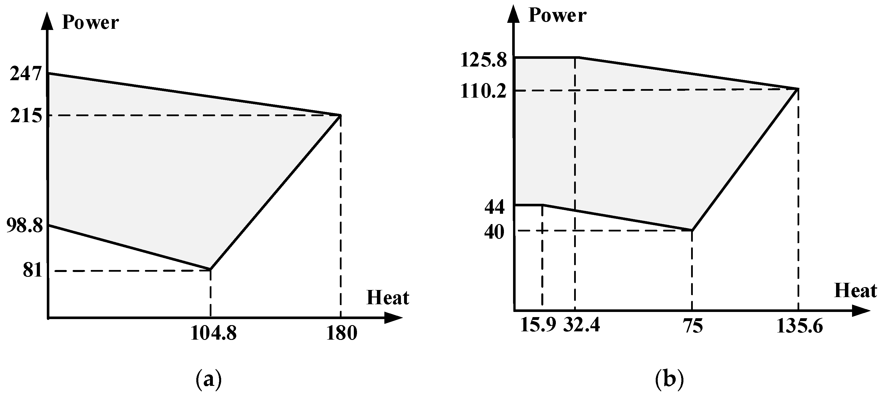
Moreover, the heat-power FOR of the CHP unit 1 and CHP unit 2 are provided in Figure 5 Mohammadi-Ivatloo et al. [12].

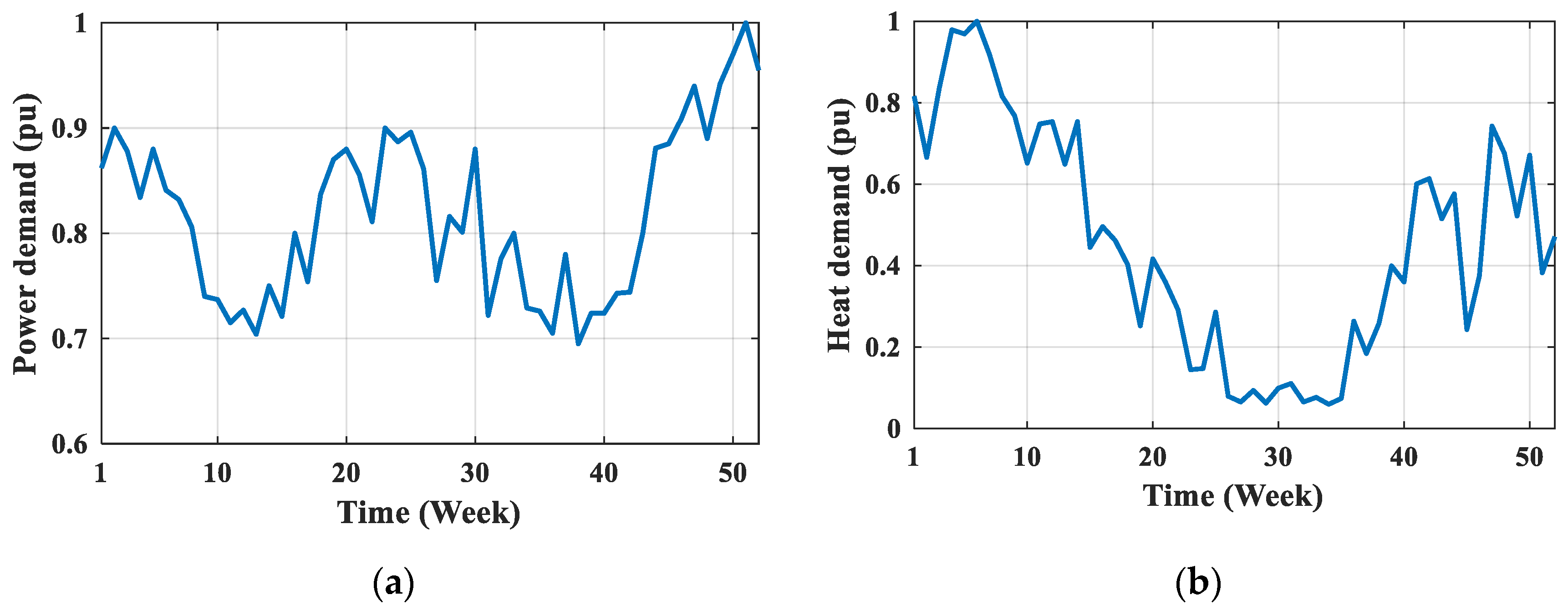
For the short-term generation scheduling, first, the long-tern GMS should be studied to determine the maintenance schedule. It is worth mentioning that in short-term scheduling, each unit that is under yearly maintenance does not participate in power or heat generation. It is clear that the power and heat demands vary due to changes in needed power and heat caused by changes in air temperature and space heating requirements. The long-term power and heat profiles for the understudy systems are as Figure 6. These per-unit profiles are multiplied with the base power and heat demands that are 350 MW and 450 MWth, respectively.

As mentioned, the long-term problem is optimized to determine the maintenance schedule that is needed for short-term generation scheduling.

Table 4. Optimal generation of the units.

Time (Week)	Power-Only Unit (MW)	CHP Unit 1		CHP Unit 2		Heat-Only Unit (MWth)
		Power (MW)	Heat (MWth)	Power (MW)	Heat (MWth)
1	27.33	148.57	97.64	125.80		269.52
2	32.08	157.12	30.04	125.80		269.52
3	34.05	147.45	106.54	125.80		269.52
4	21.79	144.31	140.33	125.80	30.70	269.52
5	38.93	143.27	139.56	125.80	26.88	269.52
6	20.00	149.30	143.13	125.05	37.35	269.52
7	20.58	144.82	127.36	125.80	16.18	269.52
8		156.30	97.64	125.80		269.52
9		133.20	75.94	125.80		269.52
10		132.15	23.70	125.80		269.52
11	97.80	152.45	67.04			269.52
12	102.32	152.13	69.56			269.52
13	88.32	158.08	22.40			269.52
14	110.37	152.13	69.56			269.52
15	91.43	160.92				200.16
16		154.20	0.81	125.80		222.30
17		138.10	4.09	125.80		203.72
18		167.15		125.80		181.04
19	20.00	158.70		125.80		113.44
20	21.28	160.92		125.80		187.38
21	20.00	153.80	0.89	125.80		161.02
22		158.05	0.03	125.80		131.28
23	28.28	160.92		125.80		65.02
24	23.73	160.92		125.80		66.28
25	26.88	160.92		125.80		128.74
26	20.00	155.55	0.53	125.80		35.15
27		138.45	4.02	125.80		25.32
28		159.80		125.80		42.08
29		154.55	0.74	125.80		27.30
30	21.28	160.92		125.80		44.64
31		126.90	6.37	125.80		43.35
32		145.80	29.34	125.80
33		154.20	34.42	125.80
34		129.35	26.78	125.80
35		128.30	33.16	125.80
36	120.95			125.80		118.58
37	147.20			125.80		82.84
38	117.45			125.80		116.01
39	127.60			125.80		179.73
40	127.60			125.80		161.91
41	134.25			125.80	0.75	269.52
42		134.60	6.60	125.80		269.52
43		154.20	0.81	125.80		230.94
44	21.63	160.92		125.80		259.29
45	23.03	160.92		125.80		109.40
46	31.43	160.92		125.80		169.02
47	50.47	152.73	64.74	125.80		269.52
48	29.09	156.60	34.14	125.80		269.52
49	42.98	160.92		125.80		234.81
50	56.90	156.80	32.61	125.80		269.52
51	63.28	160.92		125.80		172.08
52	47.53	160.92		125.80		211.86

lists the power generation of units in the long-term plan. As can be seen from the obtained results in this table, the CHP units operate in their FOR and do not deviate from that. It is worth noting that the global optimal solution has been obtained by GAMS for the understudy system.

Table 5. Total cost of the long-term plan.

	Power-Only Unit	CHP Unit 1	CHP Unit 2	Heat-Only Unit	System
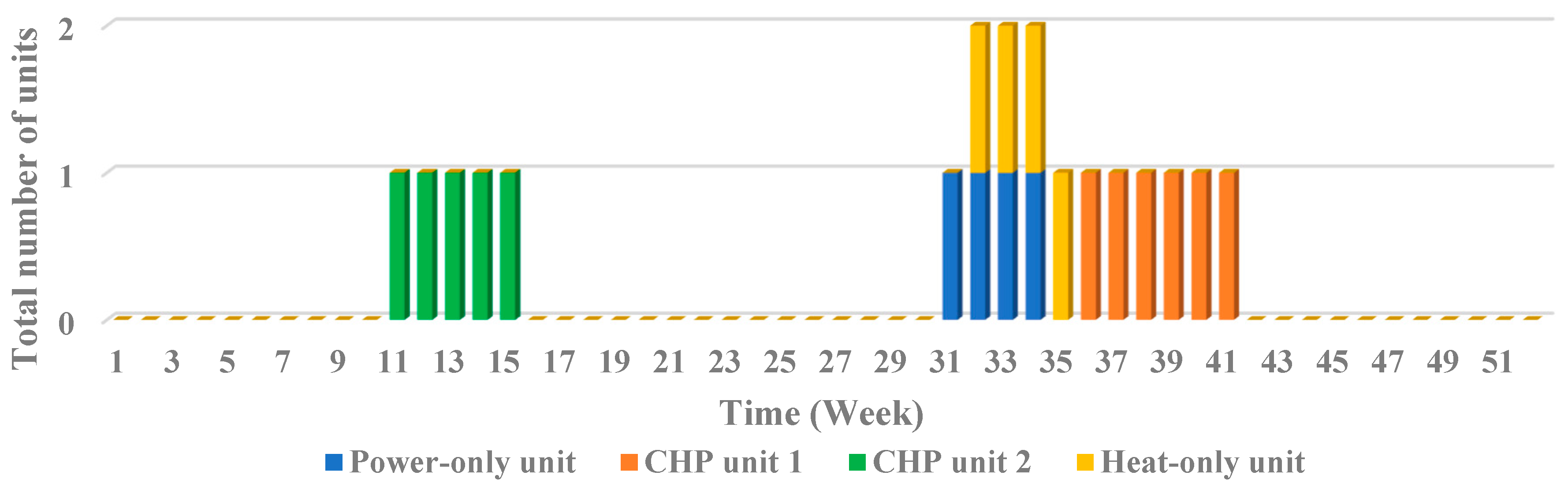
Cost (M$)	18.88197802	60.87697027	22.95173059	3.78239233	106.49307121

depicts the cost of different units in the long-term plan as well as the total cost. The yearly maintenance plan is illustrated in Figure 7. It can be seen from this figure that the power-generating units (power-only and the CHP units) are not under-maintenance simultaneously. Likewise, the maintenance intervals of heat-generating units (heat-only and the CHP units) are not simultaneous. Also, it can be seen that the maintenance interval of each unit is consecutive. As mentioned, during these weeks, the units do not participate in power or heat generation and they are out of task for the maintenance services. This figure indicates that the optimal maintenance interval of power-only, CHP 1, CHP 2, heat-only units are in weeks 31–34, 36–41, 11–15, and 32–35.

Based on the obtained maintenance intervals, some days are selected for the short-term generation scheduling. The results are presented in three cases as Case I: a day with 1 under-maintenance unit (located in weeks 15, 31, 35, 41); Case II: a day with 2 under-maintenance unit (located in week 32); and Case III: a day with no under-maintenance unit (located in week 51). The load factor for these weeks is presented in

Table 6. Demand factors for the selected weeks.

Case	Week	Under-Maintenance Unit(s) (Based on Figure 7)	Demand Factors (Based on Figure 6)
			Power	Heat
Case I	15	CHP unit 2	0.721	0.4448
	31	Power-only unit	0.722	0.1105
	35	Heat-only unit	0.726	0.0737
	41	CHP unit 1	0.743	0.6006
Case II	32	Power-only unit & Heat-only unit	0.776	0.0652
Case III	51	–	1	0.3824

.

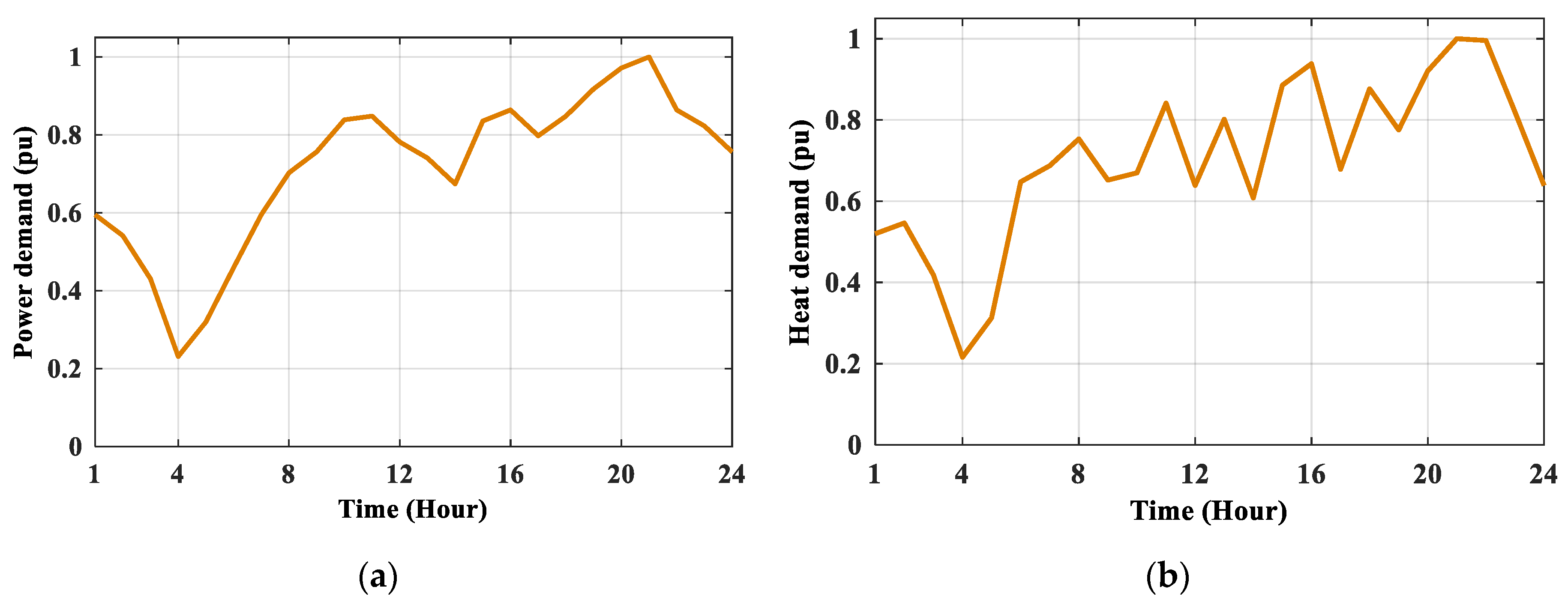
The per-unit profiles of power and heat demands are illustrated in Figure 8 Alipour et al. [52]. These profiles are multiplied with the mentioned base power and heat demands of system (350 MW and 450 MWth, respectively) and the power and heat demand factors of the related week (based on Table 6) to form the real power and heat demand.

3.1. Case I

For this case, days in weeks 15, 31, 35, and 41 are selected for short-term generation scheduling. First, a day in week 15 is selected. On this day, CHP unit 2 is under maintenance. Therefore, this unit does not participate in power or heat generation.

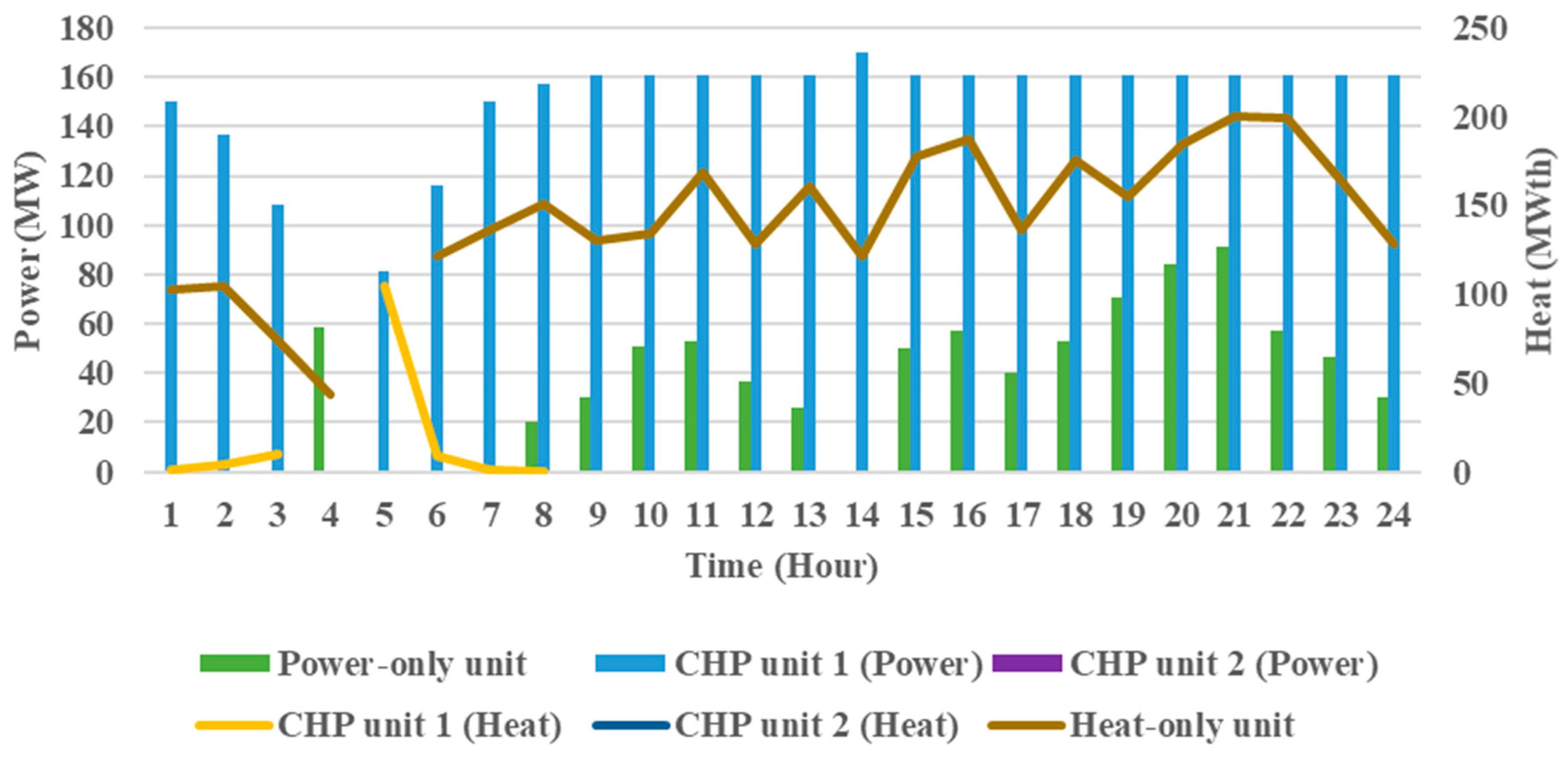
The generated power by the units is depicted in Figure 9. As this figure illustrates, the CHP unit 2 does not participate in power and heat generation. This figure also shows that the CHP units operate in their FOR. As observed, the power demand is mainly supplied by the CHP unit 1 while the heat demand is mainly supplied by the heat-only unit.

Table 7. Total cost of the short-term plan for a typical day in week 15.

	Power-Only Unit	CHP Unit 1	CHP Unit 2	Heat-Only Unit	System
Total cost (k$)	42.74030	152.29693	6.5520	7.67932	209.26855

tabulates the total cost of different units as well as the total cost of the system. It is worth mentioning that the obtained cost for the CHP unit 2 includes the fixed and maintenance costs.

For more evaluation of the obtained results, demand response is implemented. A different participation percent is considered in this research.

Table 8. The units’ cost for different participation percent in demand response for a typical day in week 15.

Participation in Demand Response	Optimal Cost (k$)
	Power-Only Unit	CHP Unit 1	CHP Unit 2 (under Maintenance)	Heat-Only Unit	System
0%	42.74030	152.29693	6.55200	7.67932	209.26855
5%	41.01164	153.74652	6.55200	7.69636	209.00652
10%	39.48881	155.03358	6.55200	7.72654	208.80093
15%	38.04201	156.28226	6.55200	7.80925	208.68552
20%	33.26298	160.96853	6.55200	7.74252	208.52603
25%	31.74955	162.16932	6.55200	7.75467	208.22554
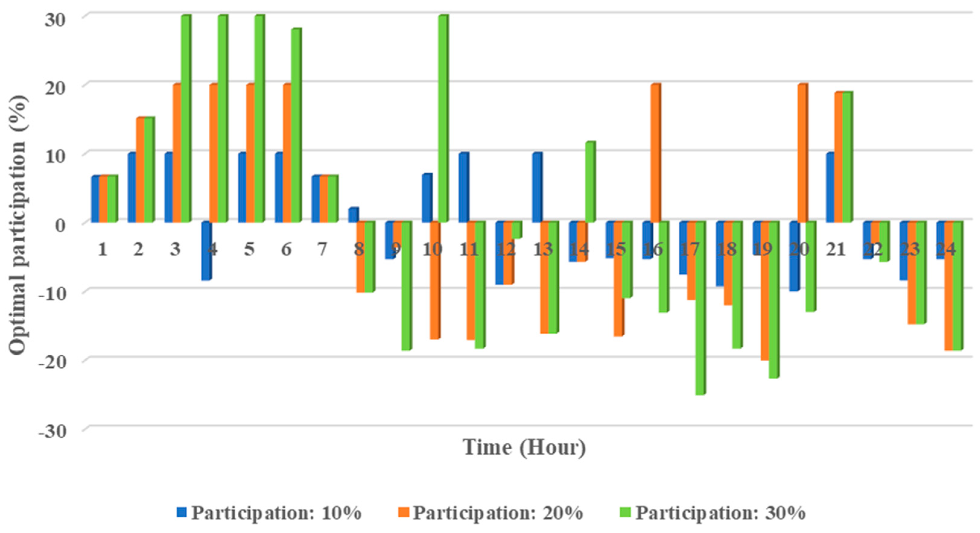
30%	30.24424	163.35240	6.55200	7.76505	207.91369

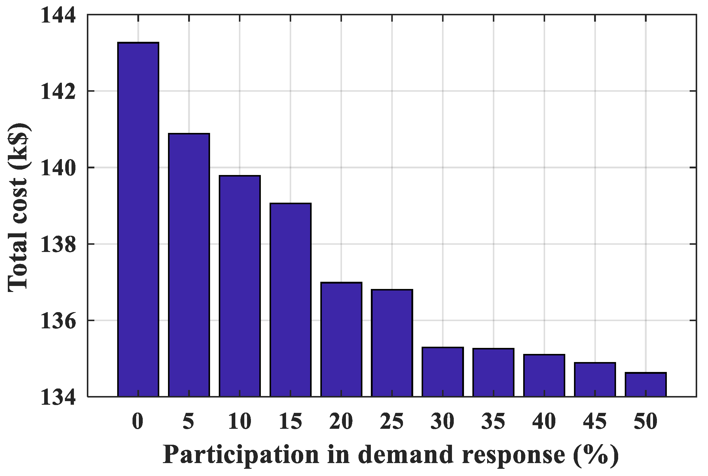
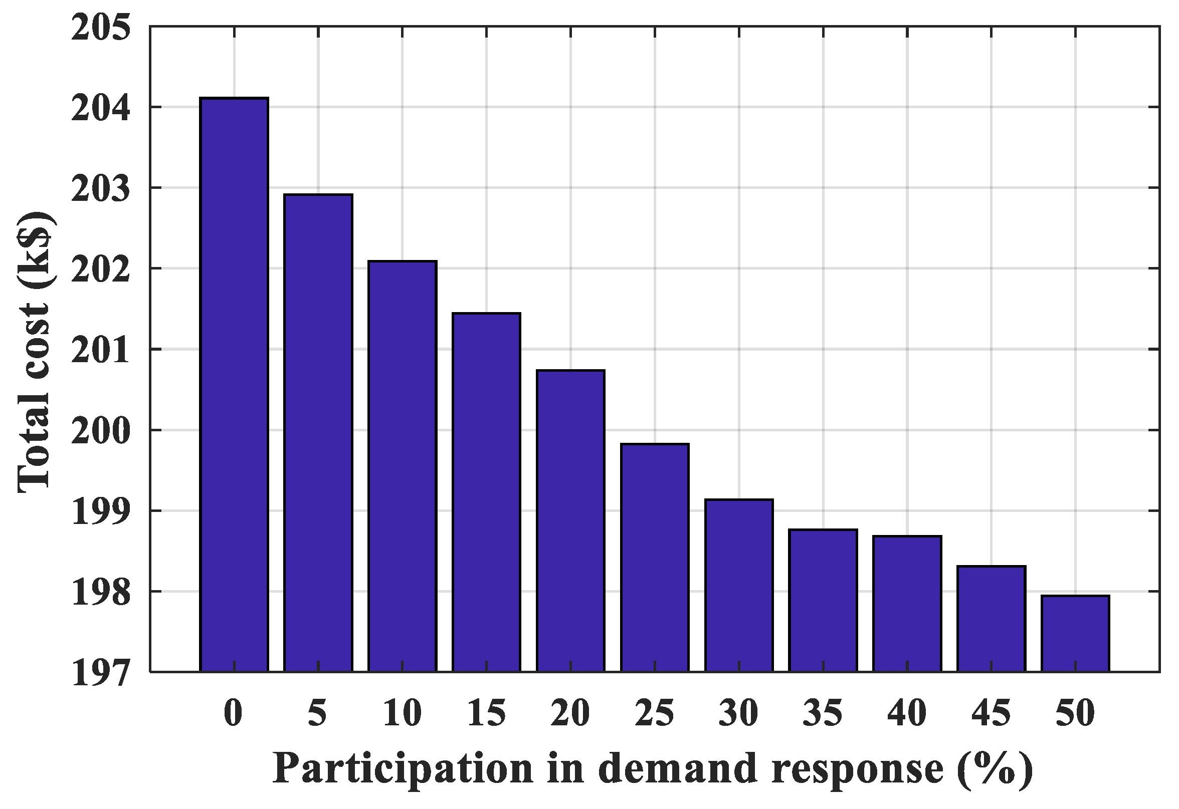
lists the optimal cost of the power-only, CHP, and heat-only units for different participation percent in demand response. As can be seen, the optimal cost of the units is changed respect to participation percent. Improving trend of the total cost of the system is also observed in this table. As mentioned, the cost of CHP unit 2 is related to the fixed and maintenance costs. In Figure 10, optimal hourly participation percent in demand response is illustrated. As observed, based on the cost optimization, the hourly loads are shifted to other hours. Additionally, it can be seen from this figure that the values of the shifted loads are not identical for different hours. Decreasing trend of the total cost respect to participation percent is shown in Figure 11. This figure shows the system cost for participation percent in the range of (0–50%) in demand response. The value of the improved cost is not uniform for identical intervals of participation percent and vary with percent and with problem.

For the other days of Case I (located in weeks 31, 35, and 41), the short-term generation scheduling is presented in

Table 9. The units’ cost for different participation percent in demand response for typical days in the weeks 31, 35, and 41.

Week of the Selected Day	Participation Percent	Optimal Cost (k$)
		Power-Only Unit	CHP Unit 1	CHP Unit 2	Heat-Only Unit	System
31	0%	0.16800	81.73645	50.75306	0.49301	133.15052
	15%	0.16800	74.85815	53.93323	0.29851	129.25789
	30%	0.16800	67.28533	57.93544	0.38956	125.77833
35	0%	8.44676	63.49479	58.29588	0.12000	130.35743
	15%	6.51920	56.47739	62.93711	0.12000	126.05370
	30%	3.20326	57.58416	63.60250	0.12000	124.50992
41	0%	79.24283	3.24000	60.36658	10.64927	153.49868
	15%	76.70784	3.24000	61.45286	10.64927	152.04997
	30%	74.90289	3.24000	62.21459	10.64927	151.00675

. In each of the selected weeks, one of the units is under maintenance. As mentioned, the obtained cost for the under-maintenance units includes the fixed cost and the maintenance cost. The impact of demand response on improving the system’s cost is also seen in this table. Additionally, the total cost of the system is considerably different, arising from difference in power and demand of typical days of the selected weeks. The under-maintenance units in those weeks are another influential factor on the total cost of the system.

3.2. Case II

In this case, a day with two under-maintenance units is selected. A typical day in week 32 is considered. Based on constraints (18) and (19), the power-generation units cannot be under-maintenance simultaneously. Likewise, the heat-generation units cannot be under-maintenance in a week. 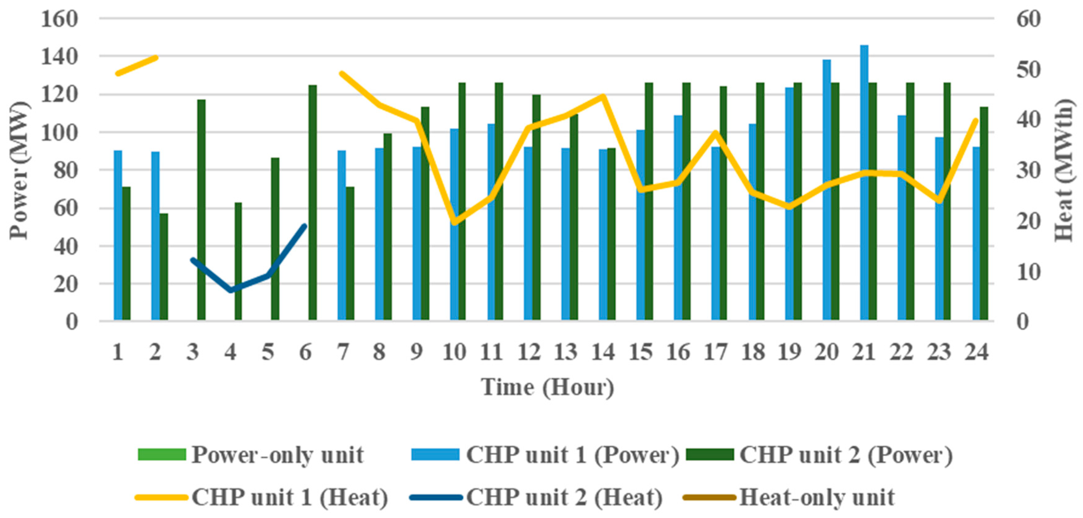Therefore, undoubtedly, the two units that are under maintenance in week 32 are power-only and heat-only units so that the system reliability not to be exposed to risk (Figure 7 confirms this issue.). Generation scheduling ignoring demand response is illustrated in Figure 12. As this figure shows, the CHP units operate in their FOR zone. In

Table 10. The units’ cost for different participation percent in demand response for a typical day in the week 32.

Participation in Demand Response	Optimal Cost (k$)
	Power-Only Unit (Under Maintenance)	CHP Unit 1	CHP Unit 2	Heat-Only Unit (Under Maintenance)	System
0%	0.16800	87.98230	54.99610	0.12000	143.26640
15%	0.16800	80.13270	58.63826	0.12000	139.05896
30%	0.16800	71.93489	63.06596	0.12000	135.28885

, the obtained costs for different participation percent of demand response is depicted for this day. Figure 13 depicts the decreasing trend of the total cost with respect to participation percent in demand response.

3.3. Case III

Finally, in this case, the generation scheduling is accomplished for a day that no unit is under maintenance. For this aim, a day in week 51 (peak power demand of the year) is selected.

Table 11. Optimal generation of the units.

Time (Hour)	Power-Only Unit (MW)	CHP Unit 1		CHP Unit 2		Heat-Only Unit (MWth)
		Power (MW)	Heat (MWth)	Power (MW)	Heat (MWth)
1		84.90	81.85	123.33		7.60
2		84.21	85.88	105.18		8.12
3	24.83			125.80		72.02
4				80.85		37.14
5				111.87		53.82
6	34.80			125.80		111.44
7		84.90	81.85	123.33		36.41
8		120.09	7.76	125.80		121.87
9		138.91	3.92	125.80		108.27
10		167.71		125.80		115.23
11	20.00	151.04	1.46	125.80		143.33
12		147.78	2.13	125.80		107.79
13		133.38	5.05	125.80		132.91
14		110.12	9.79	125.80		94.82
15		166.60		125.80		152.37
16	20.00	156.57	0.32	125.80		161.14
17		153.31	0.99	125.80		115.75
18	20.00	151.04	1.46	125.80		149.39
19	34.48	160.92		125.80		133.42
20	53.31	160.92		125.80		158.43
21	63.28	160.92		125.80		172.08
22	20.00	156.57	0.32	125.80		171.00
23		162.17		125.80		141.00
24		138.91	3.92	125.80		106.00

illustrates the generation scheduling for this day. As observed, all the units participate in demand supply and also the CHP units operate in their FOR zone. The CHP unit 2 participates in power and heat generation due to its lower cost. The improving trend of the system cost respect to participation percent in demand response is shown in Figure 14. The impact of participation percent is more for the lower participation percent. However, a higher participation percent has a lower cost. In

Table 12. The units’ cost for different participation percent in demand response for a typical day in week 51.

Participation in Demand Response	Optimal Cost (k$)
	Power-Only Unit	CHP Unit 1	CHP Unit 2	Heat-Only Unit	System
0%	14.53541	122.08611	61.37628	6.11055	204.10835
15%	2.00000	130.89263	62.09062	6.46068	201.44393
30%	0.00000	129.66859	63.00707	6.45940	199.13506

, the total cost of the units as well as the system cost are listed for 0%, 15%, and 30% participation in demand response. As seen, the cost of the power-only unit for 30% participation in demand response is 0 for the considered day because the power-only unit is not under maintenance and so it has not maintenance cost. Additionally, this unit has not fixed cost based on its data (presented in Table 1). Therefore, when this unit is off while it is not under maintenance, its cost will be 0.

For more evaluation of the proposed model, a 24-unit CHP-based system is adopted. This system contains of 13 power-only units, six CHP units, and five heat-only units. The data of the generation units for this system is listed in

Table 13. Generation units’ data of the second system.

							Power-only Units
Unit	α		β		γ		$P_{P,\min }^i$	$P_{P,\max }^i$	$N_P^i$
1	0.00028		8.1		550		0	680	6
2	0.00056		8.1		309		0	360	5
3	0.00056		8.1		309		0	360	5
4	0.00324		7.74		240		60	180	4
5	0.00324		7.74		240		60	180	4
6	0.00324		7.74		240		60	180	4
7	0.00324		7.74		240		60	180	4
8	0.00324		7.74		240		60	180	4
9	0.00324		7.74		240		60	180	4
10	0.00284		8.6		126		40	120	3
11	0.00284		8.6		126		40	120	3
12	0.00284		8.6		126		55	120	3
13	0.00284		8.6		126		55	120	3
							CHP units
Unit	a	b	c	d	e	f	Feasible region coordinates [$P_{CHP}^j$,$H_{CHP}^j$]		$N_{CHP}^j$
14	0.0345	14.5	2650	0.030	4.2	0.031	[98.8,0], [81,104.8], [215,180], [247,0]		6
15	0.0435	36	1250	0.027	0.6	0.011	[44,0], [44,15.9], [40,75], [110.2,135.6], [125.8,32.4], [125.8,0]		5
16	0.0345	14.5	2650	0.030	4.2	0.031	[98.8,0], [81,104.8], [215,180], [247,0]		6
17	0.0435	36	1250	0.027	0.6	0.011	[44,0], [44,15.9], [40,75], [110.2,135.6], [125.8,32.4], [125.8,0]		5
18	0.1035	34.5	2650	0.025	2.203	0.051	[20,0], [10,40], [45,55], [60,0]		3
19	0.0720	20	1565	0.020	2.34	0.040	[35,0], [35,20], [90,45], [90,25], [105,0]		4
							Heat-only units
Unit	ɳ		μ		σ		$H_{H,\min }^k$	$H_{H,\max }^k$	$N_H^k$
20	0.038		2.0109		950		0	269.52	3
21	0.038		2.0109		950		0	60	4
22	0.038		2.0109		950		0	60	4
23	0.052		3.0651		480		0	120	5
24	0.052		3.0651		480		0	120	5

[12].

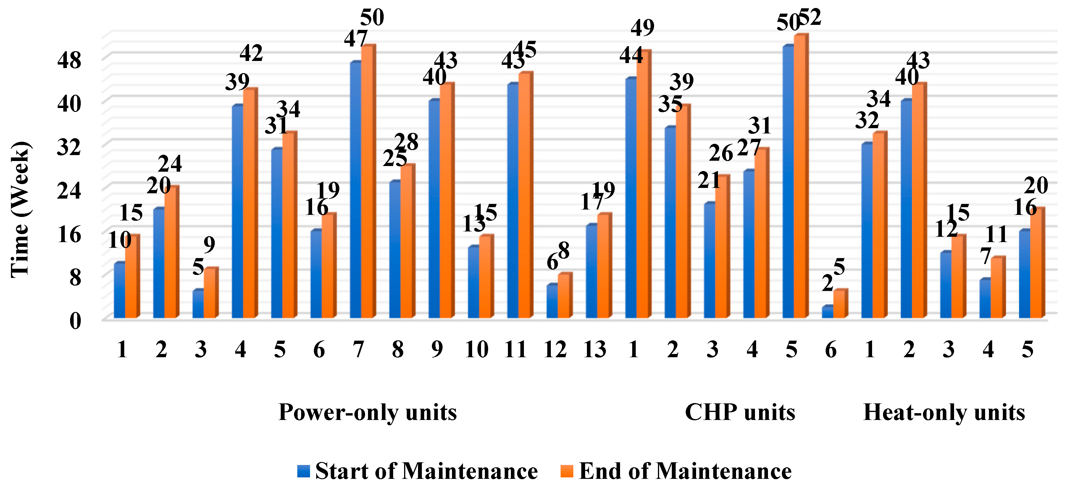
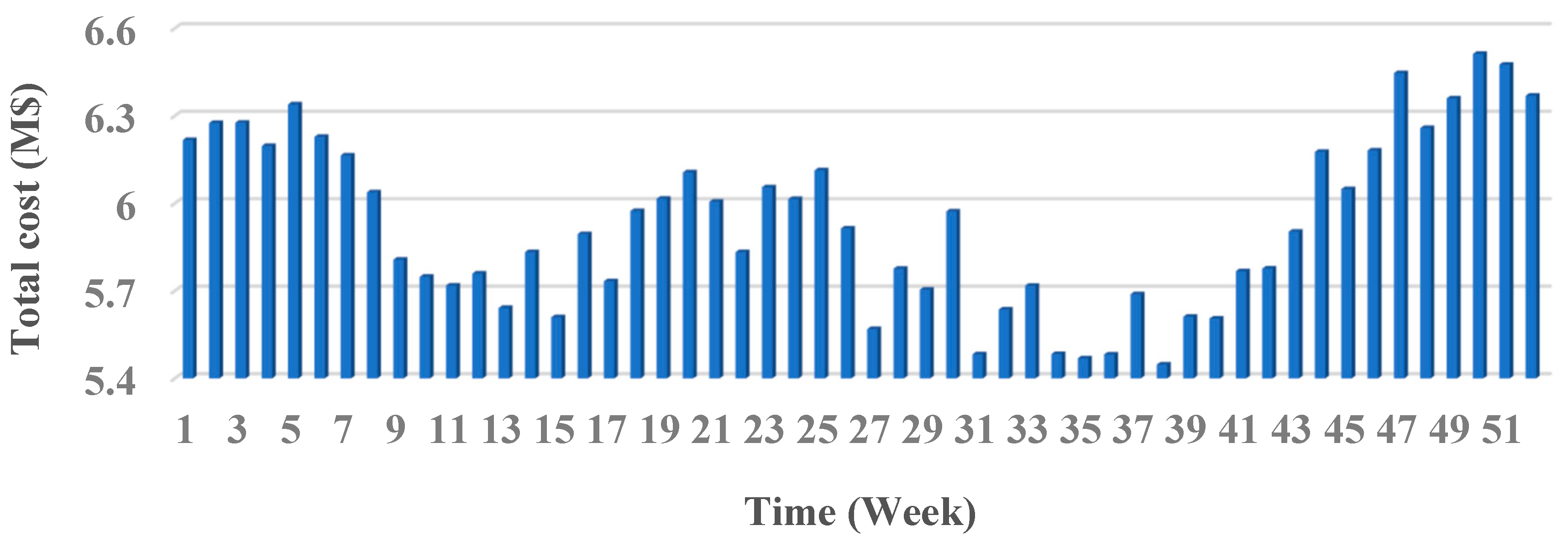
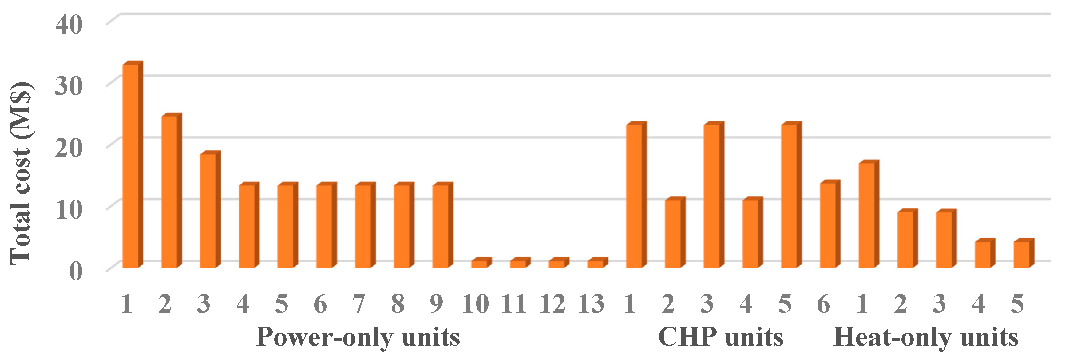
By optimizing the long-term plan, the yearly maintenance scheduling is depicted in Figure 15. The maintenance intervals are dispersed throughout the year. The maintenance interval for all the power-only, CHP, and heat-only units is shown in this figure. The total cost of the system for each week is illustrated in Figure 16. This cost includes the cost of power-only, CHP, and heat-only units that is depicted in Figure 17. As observed, the power-only units 10, 11, 12, and 13 do not participate in power generation due to their higher cost, and hence, their cost is related to the fixed and maintenance costs.

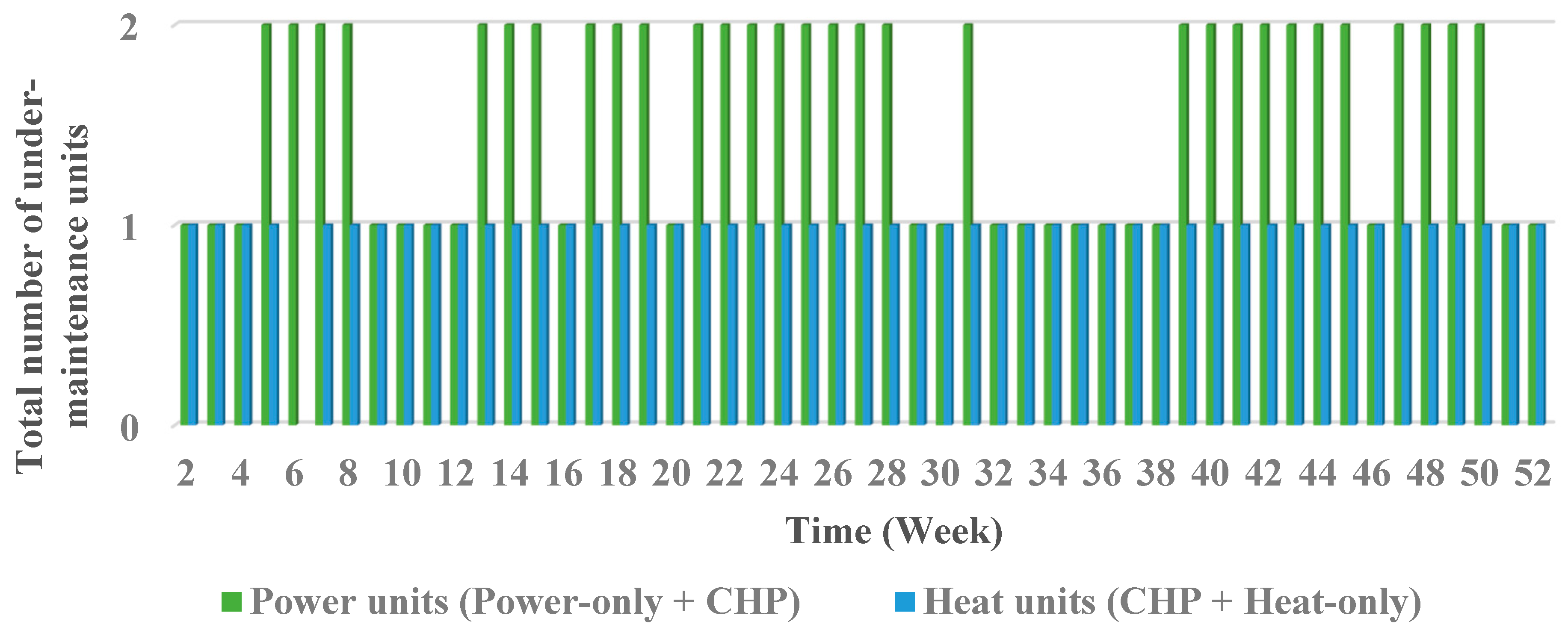
The total number of under-maintenance units is illustrated in Figure 18. As seen, the maximum number of power-producing units that are simultaneously under maintenance (i.e., 2) is greater than that of power-producing units (i.e., 1). This is due to the greater number of power-producing units. Additionally, it can be seen that constraints (18) and (19) are effective for limiting the maximum number of simultaneous under-maintenance units.

The short-term generation scheduling for the second system is studied in two cases includes Case I for week 10 and Case II for week 40. The number of under-maintenance units in these weeks is listed in

Table 14. Under-maintenance units in the selected weeks.

Case	Week	Units	Under-Maintenance Units (Based on Figure 15)
	Week 10	Power-only units	1
Case I		CHP units	–
		Heat-only units	4
	Week 40	Power-only units	4, 9
Case II		CHP units	2
		Heat-only units	–

.

3.4. Case I

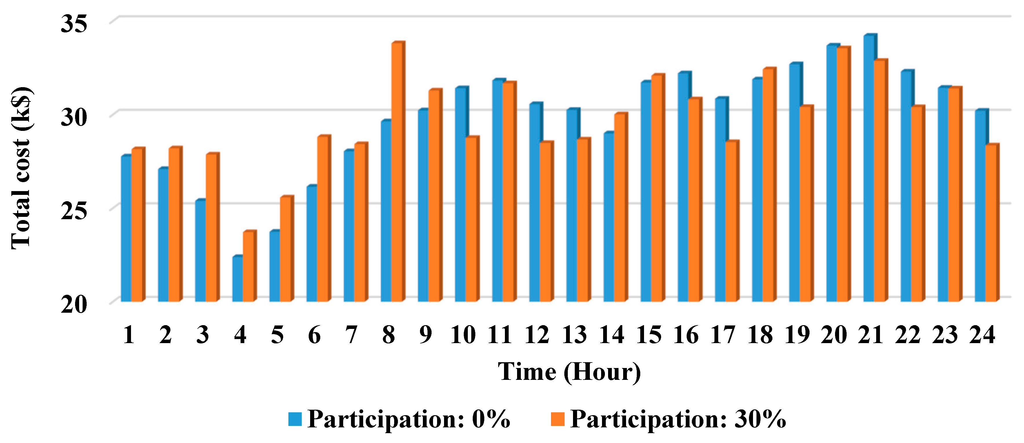
As previously mentioned, in this case, the generation scheduling of week 10 is studied. In this week, power-only unit 1 and heat-only unit 4 are under maintenance. The hourly cost of the system with respect to hour is shown in Figure 19. This figure illustrates the system cost in the presence of demand response for participation of 0% and 30%.

Table 15. The total cost of the system for different participation percent in demand response for a typical day in week 10.

Participation in Demand Response	Optimal Cost (k$)
0%	714.64241
15%	714.39687
30%	714.19046

shows the total cost of the system respect to demand response participation. As seen, demand response is effective and has improved the system cost.

3.5. Case II

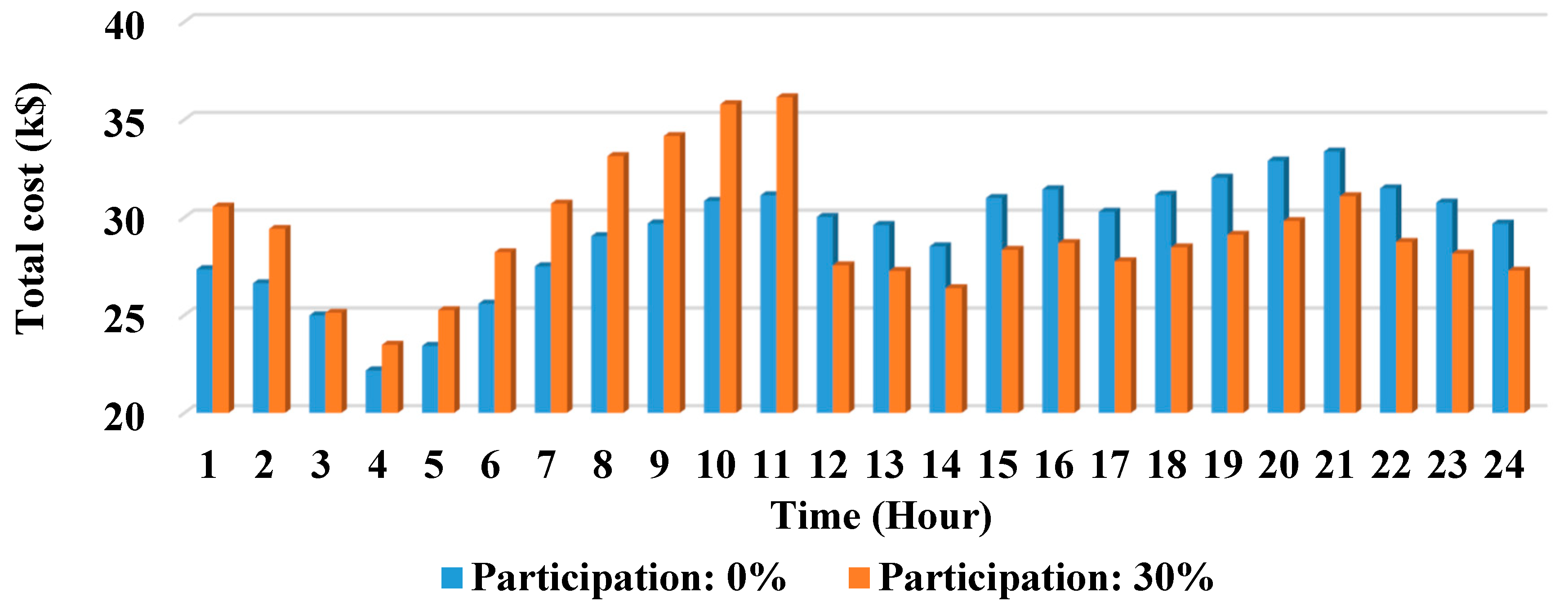
Generation scheduling of week 40 is studied in this case. In this week, power-only units 4 and 9 and CHP unit 2 are being maintenance. The system cost with respect to hour is shown in Figure 20. This figure illustrates the system cost in the presence of demand response for participation of 0% and 30%. The system cost respect to demand response participation is depicted in

Table 16. The total cost of the system for different participation percent in demand response for a typical day in week 40.

Participation in Demand Response	Optimal Cost (k$)
0%	700.58294
15%	700.52343
30%	700.45887

, which shows the effective influence of demand response on the system cost.

4. Conclusions

In this paper, the yearly preventive GMS in CHP-based systems was accomplished due to its important role in retaining network reliability as well as cost improvement. The GMS problem for power-only, CHP, and heat-only units was done with the aim to minimize the total cost of the system. The security constraints like the FOR of CHP units and demand balances for electricity and heat loads were considered. In this research, the short-term generation scheduling of the units was performed subject to the obtained yearly maintenance. The under-maintenance units did not participate in power or heat generation. The impact of demand response on generation scheduling was also investigated in this research. The resulting MIQP model was implemented in the GAMS software package and solved by the SCIP solver. Numerical simulation was accomplished to validate the effectiveness of the suggested model.

The obtained results revealed that the yearly maintenance scheduling impacts the total cost of the generating units and system in the short-term generation scheduling. The units that are under maintenance based on the long-term maintenance scheduling do not participate in power or heat generation in the short-term generation scheduling. It has been found that demand response impacts the mentioned costs as well as the generation scheduling of power-only, CHP, and heat-only units. In the case under study, CHPs participated more in demand supply due to their potential for simultaneous power and heat generation.

References

1. Salgado, F.; Pedrero, P. Short-term operation planning on cogeneration systems: A survey. Electr. Power Syst. Res. 2008, 78, 835–848. [Google Scholar] [CrossRef]
2. Mirzaei, M.A.; Nazari-Heris, M.; Mohammadi-Ivatloo, B.; Zare, K.; Marzband, M.; Anvari-Moghaddam, A. Hourly Price-Based Demand Response for Optimal Scheduling of Integrated Gas and Power Networks Considering Compressed Air Energy Storage. In Demand Response Application in Smart Grids; Springer International Publishing: Cham, Switzerland, 2020; pp. 55–74. [Google Scholar]
3. Sadeghian, O.; Mohammadpour Shotorbani, A.; Mohammadi-Ivatloo, B. Generation maintenance scheduling in virtual power plants. IET Gener. Transm. Distrib. 2019, 13, 2584–2596. [Google Scholar] [CrossRef]
4. Sadeghian, O.; Nazari-Heris, M.; Abapour, M.; Taheri, S.S.; Zare, K. Improving reliability of distribution networks using plug-in electric vehicles and demand response. J. Mod. Power Syst. Clean Energy 2019, 7, 1189–1199. [Google Scholar] [CrossRef] [Green Version]
5. Nazari-Heris, M.; Abapour, S.; Mohammadi-Ivatloo, B. Optimal economic dispatch of FC-CHP based heat and power micro-grids. Appl. Therm. Eng. 2017, 114, 756–769. [Google Scholar] [CrossRef]
6. Ahmadi, S.E.; Rezaei, N. A new isolated renewable based multi microgrid optimal energy management system considering uncertainty and demand response. Int. J. Electr. Power Energy Syst. 2020, 118, 105760. [Google Scholar] [CrossRef]
7. Rafinia, A.; Moshtagh, J.; Rezaei, N. Towards an enhanced power system sustainability: An MILP under-frequency load shedding scheme considering demand response resources. Sustain. Cities Soc. 2020, 59, 102168. [Google Scholar] [CrossRef]
8. Majidi, M.; Nojavan, S.; Zare, K. A cost-emission framework for hub energy system under demand response program. Energy 2017, 134, 157–166. [Google Scholar] [CrossRef]
9. Oshnoei, A.; Khezri, R.; Muyeen, S.M. Model predictive-based secondary frequency control considering heat pump water heaters. Energies 2019, 12, 411. [Google Scholar] [CrossRef] [Green Version]
10. Khezri, R.; Oshnoei, A.; Hagh, M.T.; Muyeen, S.M. Coordination of heat pumps, electric vehicles and AGC for efficient LFC in a smart hybrid power system via SCA-based optimized FOPID controllers. Energies 2018, 11, 420. [Google Scholar] [CrossRef] [Green Version]
11. Nazari-heris, M.; Mohammadi-ivatloo, B.; Gharehpetian, G.B. A comprehensive review of heuristic optimization algorithms for optimal combined heat and power dispatch from economic and environmental perspectives. Renew. Sustain. Energy Rev. 2017, 1–16. [Google Scholar] [CrossRef]
12. Mohammadi-ivatloo, B.; Moradi-dalvand, M.; Rabiee, A. Combined heat and power economic dispatch problem solution using particle swarm optimization with time varying acceleration coefficients. Electr. Power Syst. Res. 2013, 95, 9–18. [Google Scholar] [CrossRef]
13. Haghrah, A.; Nazari-Heris, M.; Mohammadi-ivatloo, B. Solving combined heat and power economic dispatch problem using real coded genetic algorithm with improved Mühlenbein mutation. Appl. Therm. Eng. 2016, 99, 465–475. [Google Scholar] [CrossRef]
14. Zou, D.; Li, S.; Kong, X.; Ouyang, H.; Li, Z. Solving the combined heat and power economic dispatch problems by an improved genetic algorithm and a new constraint handling strategy. Appl. Energy 2019, 237, 646–670. [Google Scholar] [CrossRef]
15. Nazari-heris, M.; Mohammadi-ivatloo, B.; Asadi, S.; Geem, Z.W. Large-Scale Combined Heat and Power Economic Dispatch Using a Novel Multi-Player Harmony Search Method. Appl. Therm. Eng. 2019, 154. [Google Scholar] [CrossRef]
16. Kia, M.; Setayesh Nazar, M.; Sepasian, M.S.; Heidari, A.; Siano, P. An efficient linear model for optimal day ahead scheduling of CHP units in active distribution networks considering load commitment programs. Energy 2017, 139, 798–817. [Google Scholar] [CrossRef]
17. Mazidi, M.; Rezaei, N.; Ghaderi, A. Simultaneous power and heat scheduling of microgrids considering operational uncertainties: A new stochastic p-robust optimization approach. Energy 2019, 185, 239–253. [Google Scholar] [CrossRef]
18. Lyu, Q.; Gong, H.; Yang, N.; Xu, X.; Zhang, N.; Wang, H. An evaluation method ofwind power integration in power systems with flexible combined heat and power plant. Energies 2019, 12, 4129. [Google Scholar] [CrossRef] [Green Version]
19. Zhang, G.; Cao, Y.; Cao, Y.; Li, D.; Wang, L. Optimal energy management for microgrids with combined heat and power (CHP) generation, energy storages, and renewable energy sources. Energies 2017, 10, 1288. [Google Scholar] [CrossRef]
20. Yuan, R.; Ye, J.; Lei, J.; Li, T. Integrated Combined Heat and Power System Dispatch Considering Electrical and Thermal Energy Storage. Energies 2016, 9, 474. [Google Scholar] [CrossRef]
21. Merkert, L.; Abdoul Haime, A.; Hohmann, S. Optimal scheduling of combined heat and power generation units using the thermal inertia of the connected district heating grid as energy storage. Energies 2019, 12, 266. [Google Scholar] [CrossRef] [Green Version]
22. Li, W.; Li, T.; Wang, H.; Dong, J.; Li, Y.; Cui, D.; Ge, W.; Yang, J.; Okoye, M.O. Optimal dispatch model considering environmental cost based on combined heat and power with thermal energy storage and demand response. Energies 2019, 12, 817. [Google Scholar] [CrossRef] [Green Version]
23. Wang, X.; Chen, S.; Zhou, Y.; Wang, J.; Cui, Y. Optimal dispatch of microgrid with combined heat and power system considering environmental cost. Energies 2018, 11, 2493. [Google Scholar] [CrossRef] [Green Version]
24. Dinh, B.H.; Nguyen, T.T.; Quynh, N.V.; Dai, L. Van A novel method for economic dispatch of combined heat and power generation. Energies 2018, 11, 3113. [Google Scholar] [CrossRef] [Green Version]
25. Amber, K.P.; Day, T.; Ratyal, N.I.; Kiani, A.K.; Ahmad, R. Techno, economic and environmental assessment of a Combined Heat and Power (CHP) system-a case study for a university campus. Energies 2018, 11, 1133. [Google Scholar] [CrossRef] [Green Version]
26. Waqar, A.; Tanveer, M.S.; Ahmad, J.; Aamir, M.; Yaqoob, M.; Anwar, F. Multi-objective analysis of a CHP plant integrated microgrid in Pakistan. Energies 2017, 10, 1625. [Google Scholar] [CrossRef] [Green Version]
27. Conejo, A.J.; García-Bertrand, R.; Díaz-Salazar, M. Generation maintenance scheduling in restructured power systems. IEEE Trans. Power Syst. 2005, 20, 984–992. [Google Scholar] [CrossRef]
28. Sadeghian, O.; Mohammadpour Shotorbani, A.; Mohammadi-Ivatloo, B. Risk-based stochastic short-term maintenance scheduling of GenCos in an oligopolistic electricity market considering the long-term plan. Electr. Power Syst. Res. 2019, 175, 105908. [Google Scholar] [CrossRef]
29. Dahal, K.; Al-Arfaj, K.; Paudyal, K. Modelling generator maintenance scheduling costs in deregulated power markets. Eur. J. Oper. Res. 2015, 240, 551–561. [Google Scholar] [CrossRef] [Green Version]
30. Rodriguez, J.A.; Anjos, M.F.; Cote, P.; Desaulniers, G. MILP formulations for generator maintenance scheduling in hydropower systems. IEEE Trans. Power Syst. 2018, 33, 6171–6180. [Google Scholar] [CrossRef]
31. Fotouhi Ghazvini, M.A.; Morais, H.; Vale, Z. Coordination between mid-term maintenance outage decisions and short-term security-constrained scheduling in smart distribution systems. Appl. Energy 2012, 96, 281–291. [Google Scholar] [CrossRef]
32. Froger, A.; Gendreau, M.; Mendoza, J.E.; Pinson, É.; Rousseau, L.M. Maintenance scheduling in the electricity industry: A literature review. Eur. J. Oper. Res. 2016, 251, 695–706. [Google Scholar] [CrossRef]
33. Eygelaar, J.; Lötter, D.P.; van Vuuren, J.H. Generator maintenance scheduling based on the risk of power generating unit failure. Int. J. Electr. Power Energy Syst. 2018, 95, 83–95. [Google Scholar] [CrossRef]
34. Lakshminarayanan, S.; Kaur, D. Optimal maintenance scheduling of generator units using discrete integer cuckoo search optimization algorithm. Swarm Evol. Comput. 2018, 42, 89–98. [Google Scholar] [CrossRef]
35. Parhizkar, T.; Mosleh, A.; Roshandel, R. Aging based optimal scheduling framework for power plants using equivalent operating hour approach. Appl. Energy 2017, 205, 1345–1363. [Google Scholar] [CrossRef]
36. Wang, Y.; Kirschen, D.S.; Zhong, H.; Xia, Q.; Kang, C. Coordination of Generation Maintenance Scheduling in Electricity Markets. IEEE Trans. Power Syst. 2016, 31, 4565–4574. [Google Scholar] [CrossRef]
37. Balaji, G.; Balamurugan, R.; Lakshminarasimman, L. Mathematical approach assisted differential evolution for generator maintenance scheduling. Int. J. Electr. Power Energy Syst. 2016, 82, 508–518. [Google Scholar] [CrossRef]
38. Moradzadeh, A.; Sadeghian, O.; Pourhossein, K.; Mohammadi-Ivatloo, B.; Anvari-Moghaddam, A. Improving Residential Load Disaggregation for Sustainable Development of Energy via Principal Component Analysis. Sustainability 2020, 12, 3158. [Google Scholar] [CrossRef] [Green Version]
39. García Márquez, F.P.; García-Pardo, I.P. Principal component analysis applied to filtered signals for maintenance management. Qual. Reliab. Eng. Int. 2009, 26, 523–527. [Google Scholar] [CrossRef]
40. Moradzadeh, A.; Pourhossein, K. Location of Disk Space Variations in Transformer Winding using Convolutional Neural Networks. In Proceedings of the 2019 54th International Universities Power Engineering Conference, UPEC 2019, Bucharest, Romania, 3–6 September 2019; pp. 1–5. [Google Scholar]
41. Moradzadeh, A.; Pourhossein, K. Short Circuit Location in Transformer Winding Using Deep Learning of Its Frequency Responses. In Proceedings of the 2019 International Aegean Conference on Electrical Machines and Power Electronics, ACEMP 2019 and 2019 International Conference on Optimization of Electrical and Electronic Equipment, OPTIM 2019, Istanbul, Turkey, 27–29 August 2019; pp. 268–273. [Google Scholar]
42. Moradzadeh, A.; Pourhossein, K. Application of Support Vector Machines to Locate Minor Short Circuits in Transformer Windings. In Proceedings of the 2019 54th International Universities Power Engineering Conference, UPEC 2019, Bucharest, Romania, 3–6 September 2019; pp. 1–6. [Google Scholar]
43. Moradzadeh, A.; Khaffafi, K. Comparison and evaluation of the performance of various types of neural networks for planning issues related to optimal management of charging and discharging electric cars in intelligent power grids. Emerg. Sci. J. 2018, 1, 201–207. [Google Scholar]
44. Marquez, F.P.G. An approach to remote condition monitoring systems management. In Proceedings of the IET International Conference on Railway Condition Monitoring, Birmingham, UK, 29–30 November 2006; pp. 156–160. [Google Scholar]
45. Chacón Muñoz, J.M.; García Márquez, F.P.; Papaelias, M. Railroad inspection based on ACFM employing a non-uniform B-spline approach. Mech. Syst. Signal Process. 2013, 40, 605–617. [Google Scholar] [CrossRef]
46. Sadeghian, O.; Oshnoei, A.; Nikkhah, S.; Mohammadi-Ivatloo, B. Multi-objective optimisation of generation maintenance scheduling in restructured power systems based on global criterion method. IET Smart Grid 2019, 2, 203–213. [Google Scholar] [CrossRef]
47. Lazimy, R. Mixed-integer quadratic programming. Math. Program. 1982, 22, 332–349. [Google Scholar] [CrossRef]
48. Brooke, A.; Kendrick, D.; Meeraus, A.; Raman, R.; Rosenthal, R.E. GAMS—A User’s Guide; GAMS Development Corporation: Washington, DC, USA, 1998. [Google Scholar]
49. Achterberg, T. SCIP: Solving constraint integer programs. Math. Program. Comput. 2009, 1, 1–41. [Google Scholar] [CrossRef]
50. Sadeghian, O.; Oshnoei, A.; Kheradmandi, M.; Mohammadi-Ivatloo, B. Optimal placement of multi-period-based switched capacitor in radial distribution systems. Comput. Electr. Eng. 2020, 82, 106549. [Google Scholar] [CrossRef]
51. Kunz, F.; Kendziorski, M.; Schill, W.-P.; Weibezahn, J.; Zepter, J.; Von Hirschhausen, C.; Hauser, P.; Zech, M.; Most, D.; Heidari, S.; et al. Electricity, heat, and gas sector data for modeling the German system. In Deutsches Institut für Wirtschaftsforschung; DIW: Berlin, Germany, 2017. [Google Scholar]
52. Alipour, M.; Zare, K.; Mohammadi-ivatloo, B. Short-term scheduling of combined heat and power generation units in the presence of demand response programs. Energy 2014, 1–13. [Google Scholar] [CrossRef]
Figure 1. Diagram of the system under study.
Energies 13 02840 g001
Figure 2. Feasible region of different units in the combined heat and power (CHP)-based system.
Energies 13 02840 g002
Figure 3. A typical heat-power feasible operation region (FOR) of CHP units.
Energies 13 02840 g003
Figure 4. Flowchart of the proposed methodology.
Energies 13 02840 g004
Figure 5. FOR of (a) CHP unit 1 and (b) CHP unit 2.
Energies 13 02840 g005
Figure 6. Long-term demands for maintenance scheduling. (a) Power demand [50]; (b) heat demand [51].
Energies 13 02840 g006
Figure 7. Optimal maintenance schedule.
Energies 13 02840 g007
Figure 8. Short-term demands for generation scheduling. (a) Power demand; (b) heat demand.
Energies 13 02840 g008
Figure 9. Short-term generation scheduling for a typical day in week 15.
Energies 13 02840 g009
Figure 10. Hourly shifted load percent in a typical day in week 15 for different participation percent in demand response (positive: added loads, negative: reduced loads).
Energies 13 02840 g010
Figure 11. Decreasing trend of total cost of the system for typical day in week 15 respect to demand response.
Energies 13 02840 g011
Figure 12. Short-term generation scheduling for a typical day in week 32.
Energies 13 02840 g012
Figure 13. Decreasing trend of the total cost of the system for a typical day in week 32 respect to demand response.
Energies 13 02840 g013
Figure 14. Decreasing trend of the total cost of the system for a typical day in the week 51 respects to demand response.
Energies 13 02840 g014
Figure 15. Start and end weeks of maintenance for all units of the second system.
Energies 13 02840 g015
Figure 16. Weekly total cost of the system.
Energies 13 02840 g016
Figure 17. Total cost of the units in the long-term plan.
Energies 13 02840 g017
Figure 18. Total number of under-maintenance power-producing and heat-producing units respect to week.
Energies 13 02840 g018
Figure 19. The system cost with and without demand response for a typical day in week 10.
Energies 13 02840 g019
Figure 20. The system cost with and without demand response for a typical day in week 40.
Energies 13 02840 g020