Anomaly Detection in Photovoltaic Production Factories via Monte Carlo Pre-Processed Principal Component Analysis

Abstract

This paper investigates a use case of robust anomaly detection applied to the scenario of a photovoltaic production factory—namely, Enel Green Power’s 3SUN solar cell production plant in Catania, Italy—by considering a Monte Carlo based pre-processing technique as a valid alternative to other typically used methods. In particular, the proposed method exhibits the following advantages: (i) Outlier replacement, by contrast with traditional methods which are limited to outlier detection only, and (ii) the preservation of temporal locality with respect to the training dataset. After pre-processing, the authors trained an anomaly detection model based on principal component analysis and defined a suitable key performance indicator for each sensor in the production line based on the model errors. In this way, by running the algorithm on unseen data streams, it is possible to isolate anomalous conditions by monitoring the above-mentioned indicators and virtually trigger an alarm when exceeding a reference threshold. The proposed approach was tested on both standard operating conditions and an anomalous scenario. With respect to the considered use case, it successfully anticipated a fault in the equipment with an advance of almost two weeks, but also demonstrated its robustness to false alarms during normal conditions.

1. Introduction

In recent years, predictive maintenance has been receiving an ever increasing attention and has been considered fundamental in industrial applications. In fact, it contributes to guaranteeing healthy, safe and reliable systems, as well as to avoiding breakdowns that could potentially lead to a whole system shutdown.

As known, the main benefit of Principal Component Analysis (PCA) lies in its capability to reduce the dimensionality of data by selecting the most important features that are responsible for the highest variability in the input dataset. Namely, PCA allows to concentrate the analysis on a compressed version of the original dataset without compromising the reliability and the robustness of a predictive model. Among other factors, a key quality in PCA is the inherent capability of processing large multivariate datasets as customary in industrial equipment sensor networks. As a result, PCA formed a field of choice in predictive analytics in several use cases, e.g., maritime and transport applications, as well as decision support systems in healthcare [1,2].

On the other hand, the well known disadvantage of PCA stems from the sensitivity to outliers in the data. In this respect, in the literature four known algorithms have been very recently devised in order to sort outliers’ observations out, namely the spherical principal component based algorithm, PCA based on robust covariance matrix estimation, robust PCA (ROBPCA) and the PCA projection pursuit algorithm [3].

To this end, based on measurements collected by the sensor network of a photovoltaic production plant, the paper proposes Monte Carlo (MC) simulation as the pre-processing stage to deal with outliers before applying PCA [4,5]. In this respect, the proposed approach is shown to be a valid alternative to relying on the classical Interquartile Range (IQR) method in order to omit outliers when applying PCA for anomaly detection purposes.

1.1. Related Works

Recently, the scientific community has devoted much attention to the use of data analytics and machine learning models in the operation domains, e.g., manufacturing and energy management. In particular, many applications have focused on predictive maintenance and anomaly detection [6,7,8].

In this context, industrial systems have adopted PCA for detecting anomalous scenarios in their operational processes. In particular, key performance indicators (KPIs) are usually defined starting from the PCA model in order to trigger alarms and prevent failures [9].

Many works focus on fault isolation techniques which are employed to classify different occurring errors and to isolate the system variables mostly affected by them [10]. Specifically, they often propose statistical methods for fault detection, like Hotelling $T^2$ or squared prediction errors Q [11,12].

Even though plenty of these works deal with error classification and isolation in the context of anomaly detection and predictive maintenance, other papers and practical experiments shed light on innovative strategies to pre-process the input data that will feed the predictive model. To this end, MC simulation has been largely applied for data pre-processing in order to define more robust models. For example, in [13] the authors process geodetic data by applying MC simulation to perform uncertainty modelling [14].

However, choosing the statistical method for MC simulation becomes difficult when the involved dataset is highly affected by the presence of outliers. In this respect, a robust estimation procedure has been investigated in [15]: The authors exploit the median since it provides an estimator with the highest breakdown point and it always guarantees a feasible solution for the considered optimization problem.

In general, MC simulation is used as a valid pre-processing strategy in order to successfully manage uncertainty with respect to experimental use cases in manufacturing and energy management, namely for predictive maintenance [16,17,18,19] or predictive analytics purposes [20].

Moreover, the number of data points sampled by MC simulation is another crucial parameter, since it could lead to inaccurate outputs [21]. This parameter is particularly challenging to optimize since it strongly depends on the use case and the quality of data. In [22] the authors test different MC simulations to determine the relationship between the sample size and the accuracy of the sample mean and variance.

Despite larger samples could provide for a better estimation of the input distributions, in [23] results demonstrated the need to restrict the number of MC runs to a number not greater than the sample sizes used for the input parameters, since a large number could be unnecessary or even harmful.

Despite the clear advantage of such approaches, they often still need to be validated in practice. So, to the best of the authors’ knowledge, this paper proposes the application of MC simulation to a real photovoltaic production scenario, as an effective way to pre-process the data stream coming from the sensors deployed throughout the production site.

The related literature also reports pre-processing techniques for similar anomaly detection scenarios based on the IQR method (e.g., [24]), which, however, offers only the property of outlier removal and not the additional benefit of outlier replacement that is consequential to applying MC simulation, as further discussed in Section 3.

1.2. Paper Structure

The paper is structured as follows. Section 2 provides the use case description and problem setting. In Section 3 we explain our contribution in terms of exploiting MC simulation as an innovative approach to data pre-processing with respect to the considered anomaly detection and predictive maintenance application. Later on, in Section 4 we discuss PCA for anomaly detection. Section 5 presents the experimental setup and numerical results. Finally, Section 6 concludes the paper.

2. Problem Setting

Enel Green Power needs to implement, in the production line of sun cells in the 3SUN Factory, an artificial intelligence application capable of predicting faults relative to a piece of process equipment, the so-called Automatic Wet Bench (AWB) machine, for predicting any malfunctioning of the fans that ventilate the different stations within such machine. The data collected on the Manufacturing Execution System (MES) are fed as input to the predictive analytics engine in order to predict faults.

2.1. Use Case

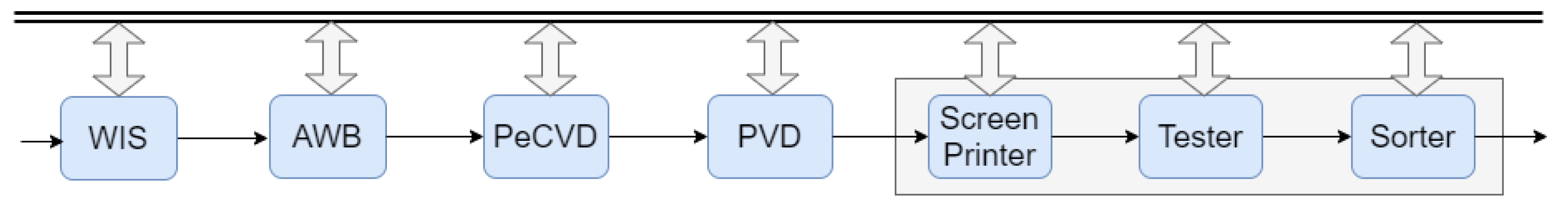
In Figure 1 we show the process steps involved in the cell production. Each process equipment has a specific purpose: Raw wafers enter the first machine in the line, the so-called Wafer Inspection System (WIS), to check the quality of the input wafers; then, they are subject to texturization and cleaning through the AWB equipment; next, the Plasma Enhanced Chemical Vapor Deposition (PeCVD) equipment is used for the deposition of doped and un-doped layer of amorphous Silicon (aSi) on both side of the wafers. Then, the Physical Vapour Deposition equipment (PVD) is used for the sputtering process. Finally, the block formed by the Screen Printer, Tester and Sorter equipment are responsible, respectively, of collecting the electric charge of the cell (fingers) and to let the flow between one cell and the other (Bus Bar) in the assembled modules, testing the electrical I-V measurements of the cells and classifying them depending on their perfomance.

The process equipment we refer to in this paper in order to predict the occurrence of faults is the AWB, where the wafers are chemically etched to roughen the surface to maximize the quantity of absorbed light and therefore the cell efficiency.

Along the production line, two parallel AWB machines are installed, each consisting of a loading station (the first one) and an unloading station (the last one) and, midway between the two, several stations where the chemical processes are performed. Within the AWB stage, the wafers are loaded onto specific containers called carriers, which move from one station to another until the process ends; the carriers do not enter in all stations but only some of them, as the same task can be carried out indifferently by one station or another, so that the carrier is moved by the automation system to the first available station that can carry out the required task.

More specifically, the stations composing the production line serve three main purposes: Pre-conditioning, texturing and cleaning. Each station is equipped with a sensor that records measurements when carriers enter and exit the station.

We now provide a brief description of the most frequently occurring fault inside the AWB and for which we design a suitable predictive analytics strategy. Such a fault is generally due to the malfunctioning of the fans that ventilate the different stations within each AWB stage.

For each AWB stage, there exist two drying tanks which must work properly in parallel and can never break down (not even alternatively), otherwise the AWB throughput would be halved, thus compromising the whole production line. Since the fault episode is generally preceded by the occurrence of anomalous vibrations, there is room for a suitable predictive analytics strategy aimed at anticipating the occurrence of the fault through the detection of such vibrations.

At a specific slot of time, an unexpected error may happen in one of its machines and block the production completely for several few days.

2.2. Sensor Measurements

The sensors mounted onto the production line stations measure several relevant parameters characterizing each station, such as station temperature, pump speed, flow speed, and ozone concentration level.

The measurements recorded by the sensors were collected only during the enter, exit and dosing phases of each carrier, thus leading to a non-constant sampling frequency. This produced many discontinuities of variable length in the sensor data streams, making standard time series analysis impossible. For this reason, the collected measurements were treated as an ordered set of samples rather than time series. In order to capture the time evolution of carriers going through a line, each sample is composed by the measurements coming from all the stations, collected during the enter, exit and dosing phases of a carrier.

Let k stations out of the total number N account for the main path drawn by a carrier entering the AWB stage to undergo pre-conditioning, texturing and cleaning. The remaining $(N-k)$ stations are parallel to the k principal ones and ensure the robustness of the whole AWB stage in the following way: If one of the k stations fails, there is at least a redundant station among the available $(N-k)$ that is properly working and can thus be entered by the carrier to undergo the whole production process.

For the sake of simplicity and without loss of generality, we assume to have k stations only, and we neglect the remaining ones. Each station contains m sensors. Each sensor measures the carrier up to t times.

The considered dataset collects the t measurements carried out by the m sensors in the k stations over n batches or carriers, assuming a batch to account for a couple of wafers flowing through the whole production line.

So we wrap all the available data into a structured dataset represented by a matrix X with n rows and $y:=k\times m\times t$ columns.

As our approach is totally data-driven, without losing generality and for the scope of the model, hereinafter we assume $k=7$ and $m=6$. Moreover, we assume $t=3$, because each sensor measures the carrier three times while it is inside the considered station.

3. Monte Carlo Based Pre-Preprocessing

In this section we illustrate a novel pre-processing approach based on Monte Carlo (MC) simulation and compare it with a commonly used method based on the Interquartile Range (IQR). This last is considered as a reference and the goal is to prove that our approach is a valid alternative to the IQR method. Since both these methods concern only the outlier removal phase, we also briefly describe the preliminary pre-processing steps required to standardize the data and handle missing values or flat signals.

3.1. Preliminary Data Cleaning

Independently on the method, a preliminary data cleaning and preparation stage is required before removing outliers. The following steps are applied:

• signal filtering when the missing values are above 5% of the total number of measurements. Above this threshold, data interpolation can lead to distortions so we preferred to discard the involved signals.
• linear interpolation of signals when the missing values are less that 5% of the total number of measurements.
• flat signals removal when the derivative is zero for at least 50% of the signal length since constant measurements do not provide any meaningful information.
• signal standardization in order to make the scales of the different signals comparable. This operation was achieved by subtracting the mean value and dividing by the standard deviation.

In the next sections we describe the reference IQR method, followed by the discussion of the proposed approach based on MC simulation.

3.2. IQR Method

The Interquartile Range (IQR) method is a simple but effective method used to identify outliers by isolating samples below the 25th percentile or above the 75th percentile [25].

3.3. Monte Carlo Method

In this paper we propose an innovative method for removing outliers based on MC simulation, which has been largely applied in other scenarios like estimation of sum, linear solvers, image recovery, matrix multiplication, low-rank approximation, etc. [26]. In our case, the idea is to generate new data points providing a more robust dataset by applying an estimator to random samples extracted from the original dataset.

By using the median estimator, there is no need to remove outliers from the raw data since this estimator is proved not to be affected by outliers [27].

Moreover, the size of the estimator dataset can be chosen arbitrarily, and can even be greater than that of the original one.

In the next sections we discuss the choice of the proper estimator, the number of samples used for MC simulation and the sliding window approach adopted to preserve the temporal locality of the sensor signals. Finally, we present the pseudocode illustrating the general pre-processing approach used to generate the new estimator dataset as input to the PCA model.

3.3.1. Mean Versus Median

The mean and the median are considered to be the most reliable estimators of the central tendency of a frequency distribution. Choosing the appropriate estimator is a challenging issue when using MC simulation since different results can lead to different correlations between signals, and thus different principal components when applying PCA. Let

$$x_i={\left(x_{p,z,w}\right)}_{\begin{array}{ccc}p& =& 1,\dots ,k\\ z& =& 1,\dots ,m\\ w& =& 1,\dots ,t\end{array}}$$

(1)

denote the i-th row of the $n\times y$ data matrix X accounting for the measurement of sensor z during phase w in station p relative to batch i. In this way, each column $f_j$ ($j=1,\dots ,k\times m\times t$) of X describes the temporal evolution of the measurements recorded by a specific sensor in a station during the processing of the batches.

Let $R^{IQR}=\left[r_{ij}^{IQR}\right]$ with $i,j\in \{1,\dots ,n\}$, $i\ne j$, $r_{ij}^{IQR}=\frac{{\sigma }_{f_i{f}_j}}{{\sigma }_{f_i}{\sigma }_{f_j}}$ and $-1\le r_{ij}^{IQR}\le 1$ denote the correlation matrix computed between the columns of the dataset resulting from the IQR pre-processing. Recall that ${\sigma }_{f_i{f}_j}$ denotes the covariance between the columns $f_i$ and $f_j$, whereas ${\sigma }_{f_i}$ denotes the variance of the i-th column.

Let $R^{MC,median}=\left[r_{ij}^{MC,median}\right]$ and $R^{MC,mean}=\left[r_{ij}^{MC,mean}\right]$$(i,j\in \{1,\dots ,n\}$, $i\ne j)$, formulated as above, denote the correlation matrix computed between the columns of the dataset resulting from the median-based and the mean-based MC simulation pre-processing methods, respectively.

Let $\Delta :=\left[{\delta }_{ij}\right]=R^{IQR}-R^{MC}$ account for the deviation between the two matrices, letting $R^{MC}$ denote alternatively the correlation matrix relative to the median-based or the mean-based MC pre-processing method.

In order to evaluate which estimator suits our purpose best, we run the following statistical hypothesis test:

$$\left\{\begin{array}{c}{H}_0:{\delta }_{ij}<\alpha \forall i,j\hfill \\ H_1:{\delta }_{ij}\ge \alpha \forall i,j,\hfill \end{array}\right.$$

(2)

considering the difference between the correlation matrix computed after the application of the IQR method and the correlation matrix of the new dataset resulting from the previous section (that is, the MC dataset).

We can state that there exists a significance level $\alpha$ such that ${\delta }_{i,j}^{MC,median}<\alpha ,\forall i,j$, and $\exists (i,j):{\delta }_{i,j}^{MC,mean}\ge \alpha$, allowing us to choose $H_0$ only under the median-based MC method.

In particular, in the considered use case, the difference in the correlation matrices considering the median-based MC method is less than $\alpha =6\times {10}^{-2}$ in absolute value and this proves to be a consequence of the median insensitivity to outlier observations.

3.3.2. Choosing the Size of the Monte Carlo Sample

Choosing the proper number of samples has a significant effect on MC simulation since it considerably improves estimation reliability. We recall that samples are chosen out of the data matrix X, where $x_i$, as defined in (1), represents a generic row of X accounting for the measurement of sensor z during phase w in station p relative to batch i.

Up to the authors’ knowledge, the literature claims that increasing the sample size reduces the variance and decreases the noise of the simulation results method [28]. Calibrating the sample size depends on many factors such as dataset size, the pursued objective and the complexity of the phenomenon the designer is modeling [29]. Therefore, we have tested different sample sizes before defining a methodology aimed at finding a suitable number of samples for each round in MC simulation.

By comparison with the highly dispersed original dataset, by increasing the number of samples we obtain a proportional decrease in variance. The desired sample size will allow to remove only the outliers and at the same time preserve the rest of the information contained in the original dataset.

By excessively increasing the number of samples, the risk is that a significant part of the information is lost, thus affecting the accuracy of the PCA model.

In order to select the proper sample size for MC-based outlier removal, we evaluate the impact this parameter has on the PCA model.

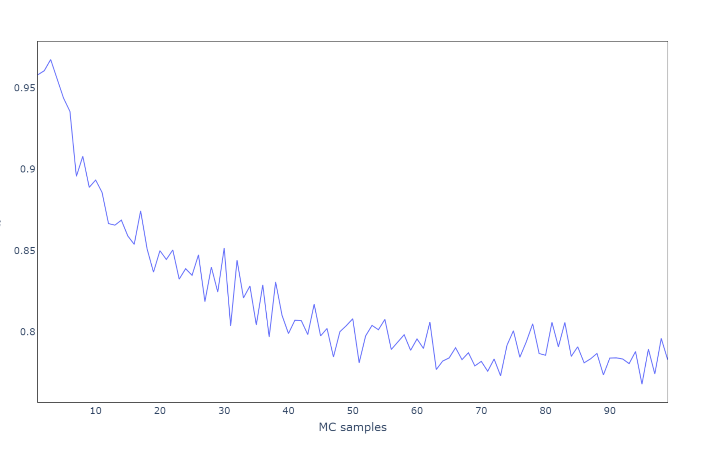
To demonstrate that MC pre-processing is a valid alternative to the IQR-based pre-processing method, we compared the PCA models resulting from both approaches for different sample sizes, ranging from 1 to 100. In particular, we measured the proportion of the variance of the MC-PCA components that is explained by the IQR-PCA components in terms of $R^2$. In this way, high values of $R^2$ correspond to similar PCA models, thus confirming the equivalent performance of the two pre-processing methods.

From Figure 2, it is evident that by considering three samples we obtain the highest value of $R^2$ (around $97.5\%$), thus demonstrating that, by choosing the proper sample size, the MC pre-processing method achieves very similar results to those obtained by the IQR-based pre-processing method.

Figure 2 presents the results of the previous steps where it is experimentally proven that PCA with three-sample size has the best results.

3.3.3. Preserving Trend Properties through a Suitable Choice of the Monte Carlo Sample

Since PCA is based on the linear correlation among variables, any trends intrinsic to the signals themselves will not be considered. For this reason, a random sampling among all the batches for the purpose of median computation may result in the loss of the temporal dependencies characterizing signals.

Therefore, we refined the procedure for the MC sample selection accordingly. In particular, for each batch in the original dataset we considered a time window centered around the batch itself. Samples considered for the median computation were therefore extracted inside such window, thus preserving the temporal locality among subsequent batches.

3.3.4. Pseudocode for the Pre-Processing Method Based on MC Simulation

The pseudocode reported in Algorithm 1 illustrates the steps required to generate a new estimator dataset by using a pre-processing procedure based on MC simulation, as proposed in Section 3.3.1–Section 3.3.3.

Algorithm 1 Pre-processing algorithm based on MC simulation

InputX: The original $n\times y$ data matrix Output$\widehat{X}$: The new estimator $\widehat{n}\times y$ data matrix Parameter$\widehat{n}$: The size of the new estimator dataset Parameterb: The number of samples considered for MC simulation i← 0 while $i<\widehat{n}$ do $idx$← generateRandomInteger [b, $n-b-1$] forj in range [0, $y-1$] do $window$←X [$idx-b$: $idx+b$, j] $\widehat{X}$[i, j] = ← median($window$) end i←i + 1 end

4. Principal Component Analysis for Anomaly Detection

Principal Component Analysis (PCA) is a well known method commonly used to reduce the dimensionality of a dataset, by transforming the original set of variables into a smaller one that still contains most of the information in terms of variance. In particular, it is a linear dimensionality reduction method based on Singular Value Decomposition (SVD) that projects the data on a lower dimensional space.

Being $\widehat{n}$ the number of samples and let y the number of variables, the $\widehat{n}\times y$ data matrix $\widehat{X}$ is centered (by removing the mean of every feature) and SVD is applied on its covariance matrix, thus leading to a subset of orthonormal dimensions, namely the Principal Components (PCs) [30]. Since SVD computes PCs incrementally, their number depends on the pre-defined stopping criterion in searching for the next PC. A common strategy is to define the number of PCs as a function of the minimum variance information to be preserved with respect to the original dataset in order to compress the data sufficiently without loosing too much information.

In this paper we use PCA to perform anomaly detection. For this purpose, it is necessary to isolate a subset of data points associated with a normal behavior of the equipment. This subset is used as input to the PCA algorithm to compute a set of PCs considering as stopping criterion a high variance preservation (at least 90%). Having defined the $y\times z$ projection matrix $\mathsf{\Pi }$ composed by the z PCs, it is now possible to project each data point ${\widehat{x}}_i$ on a lower dimensional space as:

$$c_i={\widehat{x}}_i\mathsf{\Pi }$$

(3)

where $c_i$ is the z-dimensional compressed version of ${\widehat{x}}_i$. Then, we transform $c_i$ back to its original space by multiplying it by the the inverse of the matrix $\mathsf{\Pi }$ (being $\mathsf{\Pi }$ orthonormal, the inverse coincides with its transpose), thus obtaining the reconstructed version of the input data:

$${\widehat{x}}_i^{\prime }=c_i{\mathsf{\Pi }}^T$$

(4)

Finally, we compute the reconstruction error of the sample ${\widehat{x}}_i$ as:

$$e_i=|{\widehat{x}}_i’-{\widehat{x}}_i|$$

(5)

where the vector $e_i$ contains the residual of every input feature. Since the model is trained on normal behavior data, the reconstruction error should be low for samples belonging to the same distribution. However, during an anomalous scenario, the error is expected to be high since the associated samples will deviate from such distribution. By considering these vectors as KPIs for the stations in the production lines, it is not only possible to detect anomalies when high errors occur, but also go back to the sensors mostly involved by inspecting the residuals of each single input feature.

Remark 1.

Thanks to the property of outlier replacement, to the median-based approach as introduced in Section 3.3.1, to the optimal choice of the sample size as described in Section 3.3.2 and to the preservation of any temporal dependencies characterizing the input signals as stated in Section 3.3.3, the proposed MC-based pre-processing approach turns out to be a robust alternative to IQR pre-processing. In fact, as it can be seen from the experimental results reported in Section 5, using median-based MC simulation in place of the IQR method for the pre-processing stage yields very similar results, although the number of PCs obtained when applying PCA after MC simulation is slightly higher than the number of PCs obtained when applying PCA after the IQR method.

Remark 2.

The proposed pre-processing approach based on MC simulation is more adapt to the scenario of energy plants whose data require extensive cleaning. In this respect, if the input data are not cleaned enough, the IQR method, by isolating samples below the 25th percentile or above the 75th percentile, may end up removing a significant part of the original dataset, thus potentially compromising the quality of the subsequent data analytics task. Instead, MC simulation overcomes this obstacle by enabling the data scientist to tune the dimension of the dataset resulting from pre-processing according to the technical specifications of the considered task.

5. Experimental Results of Anomaly Detection

In the experimental phase, we compared the results of the proposed anomaly detection approach considering both the IQR and MC pre-processing methods. In both scenarios, the relevant data were collected from the MES of the 3SUN Factory and a set of normal behaviour samples was defined for training the PCA model.

5.1. Training and Test Sets

According to the data format of matrix X specified in (1), we isolated a week of normal condition samples as training set, going from 8 July 2020 to 15 July 2020. This period was labelled as a period of standard operation by the operators working in the plant, together with other periods going from 1 November 2020 to 14 November 2020 and from 1 May 2020 to 8 May 2020, respectively, which we considered as test sets. The operators reported a fault in the plant on 4 July 2020, so we isolated 24 days of data before the fault as a further test set to see if the proposed model actually detects the anomaly, possibly in advance.

5.2. Pre-Processing Phase

Before the application of the anomaly detection approach based on PCA, we pre-processed the dataset as described in Section 3. In particular, 10 signals were filtered since they were completely flat, 12 signals were discarded since they presented an excessive rate of missing values, and eight signals were linearly interpolated. After this phase, the dataset counted 36 variables on which the two outlier removal methods were applied.

Outlier Removal Results

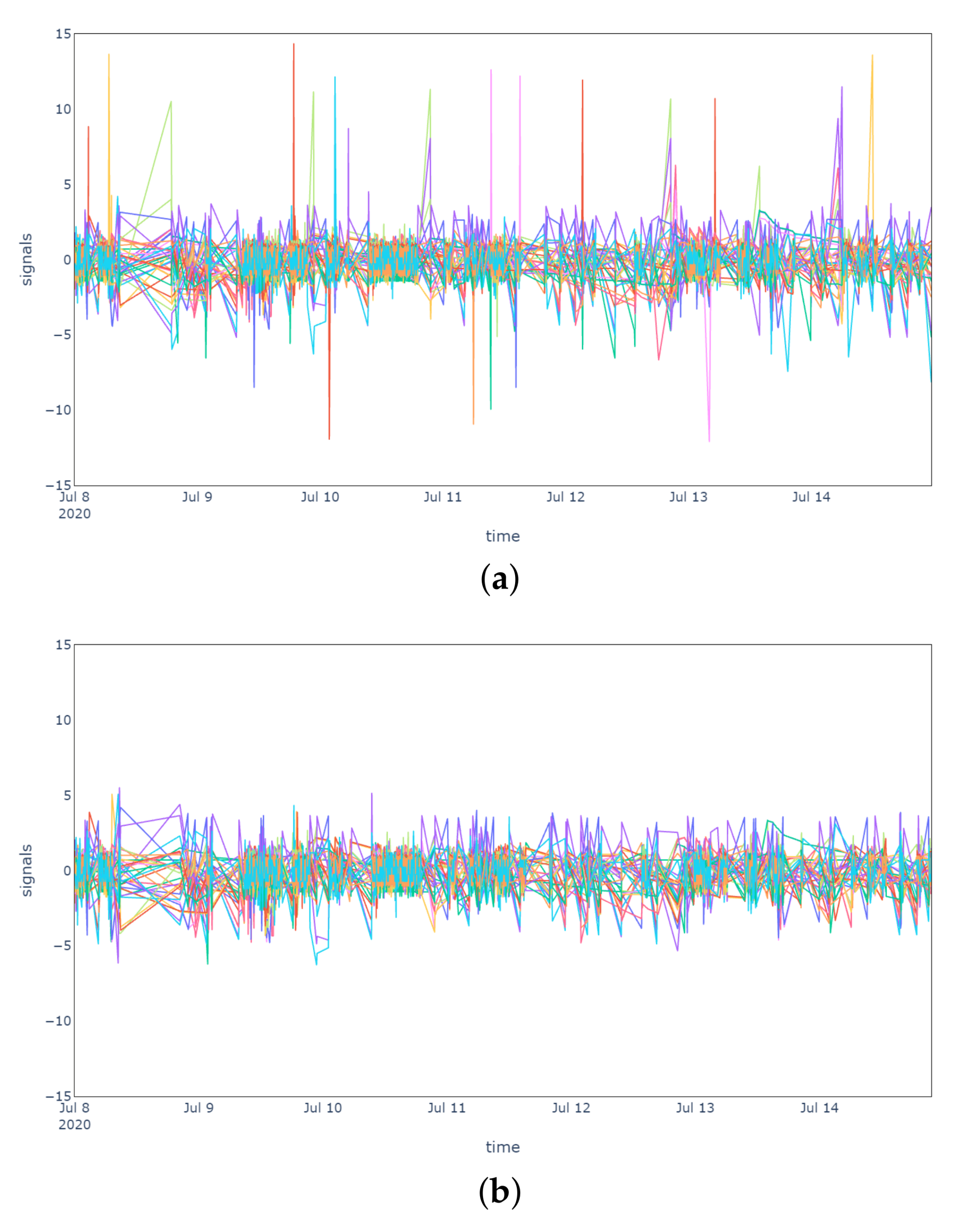
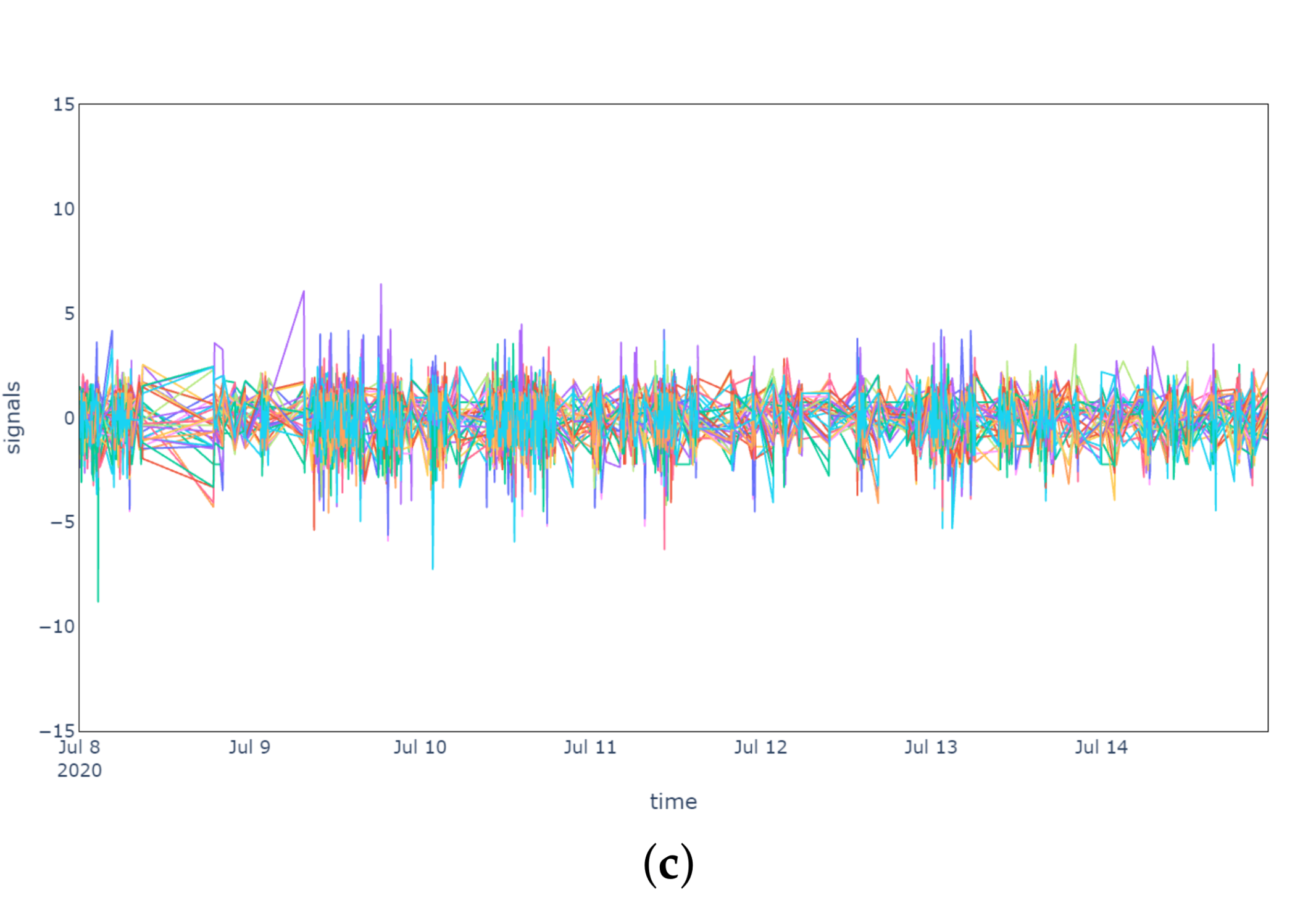
From the results it is evident that both the IQR and MC methods were able to filter outliers successfully. In Figure 3a, the original sensor signals are plotted in order to highlight the presence of outliers, while in Figure 3b,c, respectively, the pre-processed signals after the IQR and MC outlier removal methods are presented. It is important to notice that the IQR method does not handle the substitution of outliers (e.g., by interpolation) and it is limited to their identification and filtering. The MC method, instead, handles the presence of outliers by replacing all data points with the median over a sliding window, without requiring any additional substitution phase for the filtered values.

5.3. Anomaly Detection Results

The PCA algorithm was run onto the two scenarios, namely considering an IQR and MC pre-processing phase, by setting as stopping criterion a minimum of 90% of explained variance. In the case of IQR, the PCs computed by the PCA algorithm were 16, while using the MC method led to 19 new dimensions.

5.3.1. Testing in Normal Operating Conditions

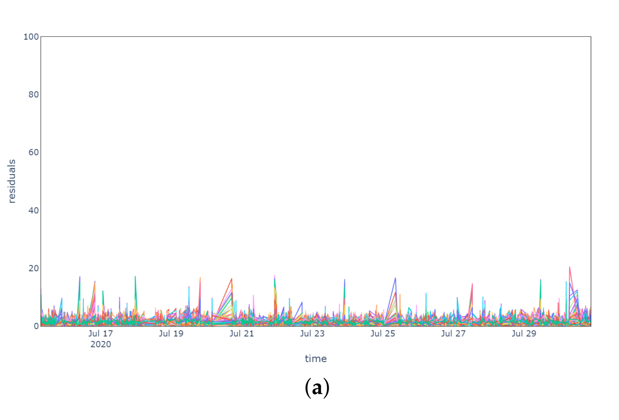
The robustness of the anomaly detection model has been tested on normal behaviour conditions (Figure 4) in a period going from 1 November 2020 to 14 November 2020, namely on the data collected during the week following the training period. Figure 4a plots the reconstruction errors of the model without pre-processing, while Figure 4b,c display, respectively, the residuals considering IQR and MC for pre-processing. In all scenarios the reconstruction errors are never persistently exceeding a threshold of 20 units, which was taken as a reference considering the errors computed on the training data. In fact, the operating conditions are very similar to the normal behaviour period on which the model was trained and demonstrate that there are no substantial differences between the two pre-processing methods.

5.3.2. Testing in Anomalous Conditions

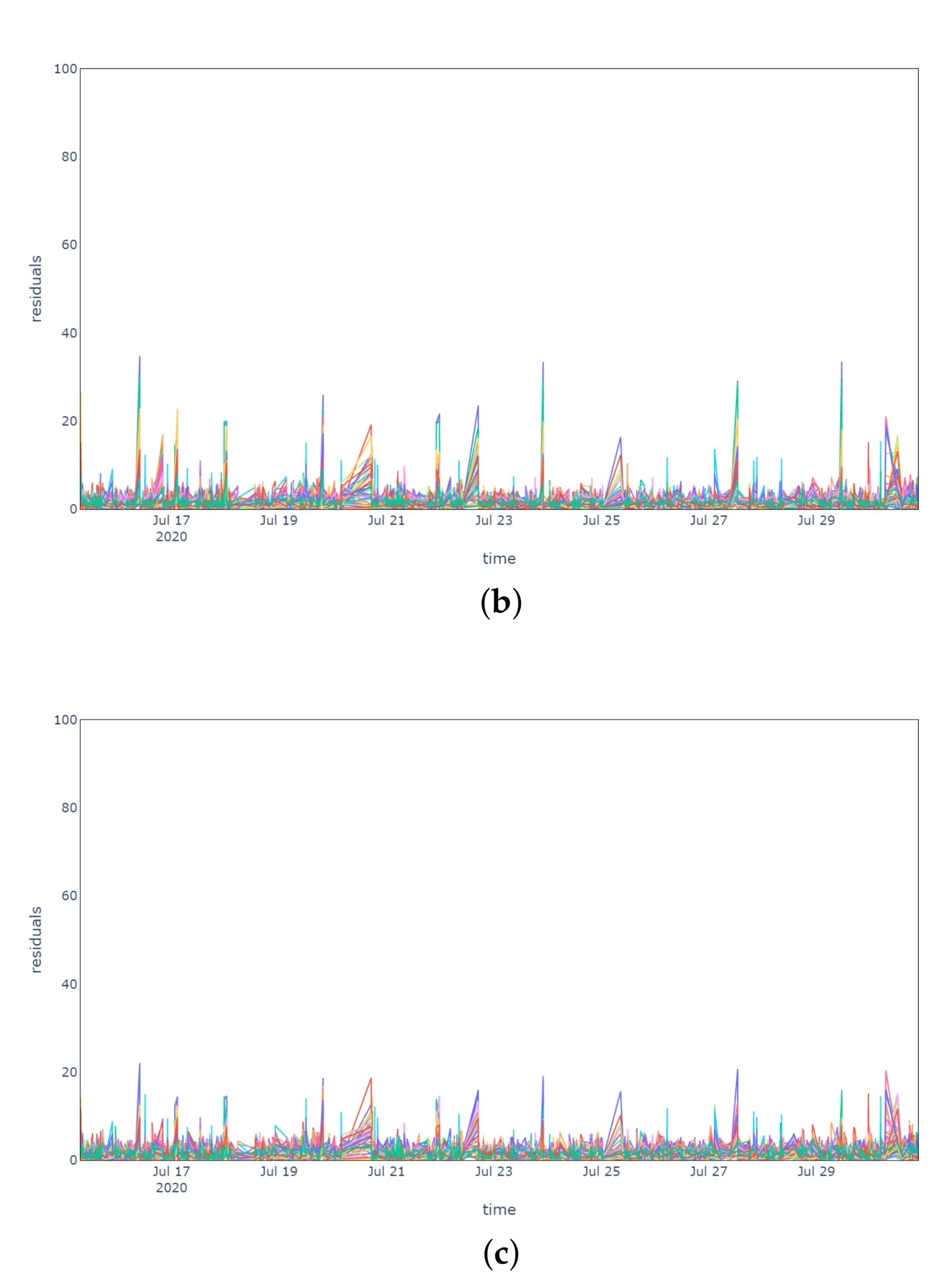
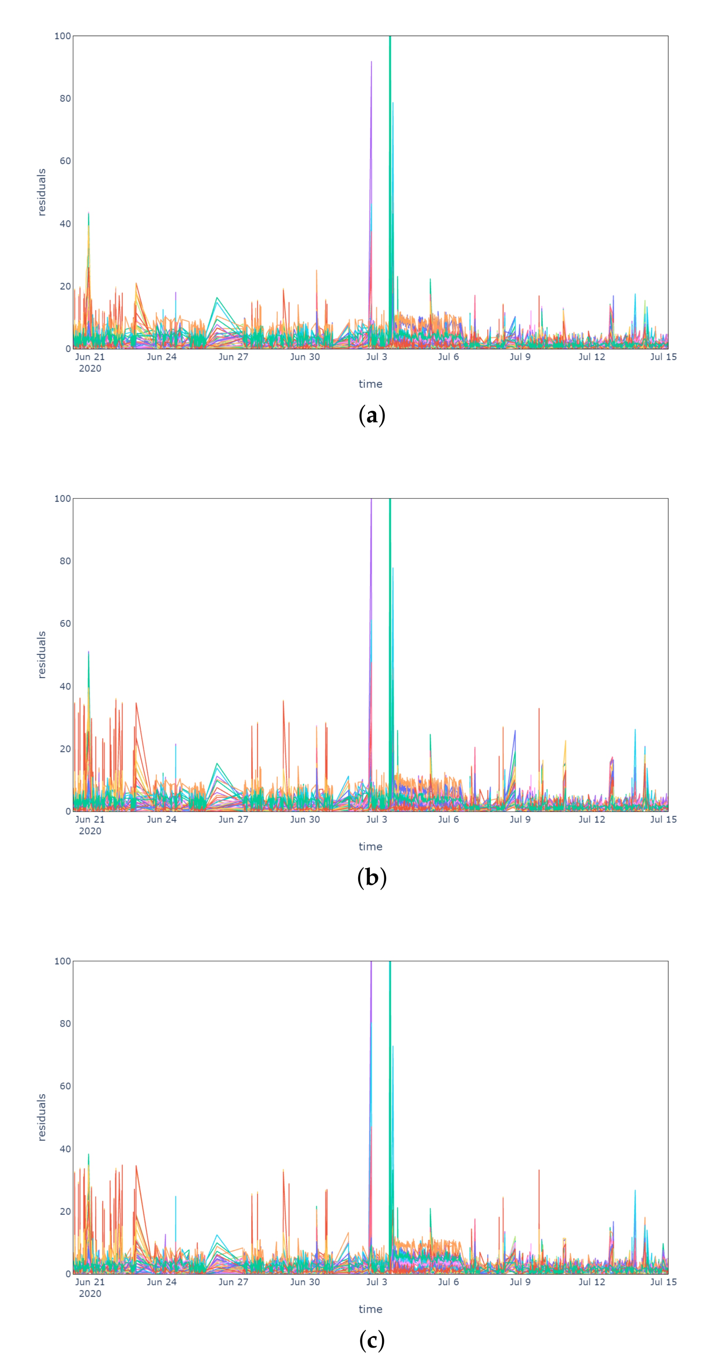
As a final step, we evaluated the model in a critical period going from 20 June 2020 to 8 July 2020, during which a technical problem led to equipment failure, as reported by the operators. Figure 5 shows the residuals of the model considering no outlier removal phase (Figure 5a), the IQR (Figure 5b) and the MC (Figure 5c) pre-processing methods. In proximity of the failure event (on 4 July 2020), the anomaly is detected by the residuals drastically exceeding the training reference threshold of 20 units, anticipated by another reconstruction error spike on 3 July 2020. Without outlier removal the residuals never persistently exceed the threshold in the period preceding the fault. When considering the IQR and MC methods, instead, residuals above 20 units are already frequent starting from 20 June 2020, anticipating the fault by more or less two weeks. As for the normal behaviour scenario, also in an anomalous period the two pre-processing methods demonstrated their similarity by achieving comparable results.

It is important to notice that it is possible to isolate the sensors of the stations that are mostly related to the anomalous conditions by inspecting the residual of each input feature of the model. In this anomalous period, stations 12 and 13 were isolated by looking at the large residuals two weeks before the fault. During the fault itself, instead, stations 19 and 20 were involved according to the model reconstruction errors.

6. Discussion

The proposed method for data pre-processing based on MC simulation exhibits the following features:

• preserving temporal locality with respect to the training dataset;
• outlier removal;
• outlier replacement, by contrast with traditional methods which are limited to outlier detection only (for example methods based on z-scores [31] or IQR techniques [32]).

As discussed in Section 3.3 and confirmed in [27], the median was chosen as the most accurate estimator in order to obtain a suitable dataset using Monte Carlo simulation to be provided as input to the PCA-based model. In particular, the median-based MC method proved to be more effective against outlier observations with respect to the mean estimator.

Moreover, we selected the optimal sample size for MC simulation by measuring the percentage of variance of the PCA components trained on the MC pre-processed dataset explained by the PCA components trained on the IQR pre-processed dataset in terms of $R^2$ due to many considerations in the literature which report pre-processing techniques for similar anomaly detection scenarios based on the IQR method [24]. This analysis led to an optimal value of three samples to be considered for the median computation. In particular, we adopted a sliding window sampling approach in order to preserve the temporal locality of subsequent batches.

From the results is Section 5.3 it is evident that the IQR and MC-based pre-processing methods produce similar results, demonstrating their capability to successfully deal with outliers. Nevertheless, they present substantial differences. In fact, a standard method like IQR is limited to isolating outliers and possibly remove them from the dataset. This is a limitation because filtered observations generate missing values which require a substitution algorithm (e.g., mean imputation [33], KNN [34], linear interpolation [35]). The MC method, instead, intrinsically deals with outlier substitution by computing the median of randomly selected points, thus generating a new estimator dataset with an arbitrary number of samples.

The PCA models for anomaly detection demonstrated their capability to successfully anticipate a fault in the equipment as shown in several other works and practical experiments [6,7,8]. In particular, two PCA models were trained, respectively, on the IQR and MC pre-processed datasets. Both models highlighted an anomalous condition almost two weeks before the equipment failure by producing KPIs (residuals) above a reference threshold which was used to discriminate between healthy and anomalous states of the equipment as done in [36].

Moreover, it is important to notice that, without any pre-processing, the algorithm is unable to detect the anomalies with such an advance and is limited to spotting only the occurrence of the actual fault, which is also detected by the IQR and MC approaches.

Both models were also tested in standard operating conditions in order to prove their robustness to false alarms. In fact, in normal conditions, the residuals of the models never exceed the reference threshold persistently.

Finally, by inspecting the residual of each input feature of the model, the proposed approach allows to isolate the sensors of the stations that are being subject to anomalous conditions.

The authors have selected a reference period in order to calculate the average downtime for the AWB stage of the production line shown in Figure 1, and then to compute an estimate of the AWB downtime reduction resulting from the adoption of our predictive model.

Considering that only 50% of the predicted machine-down events can be totally avoided—in fact, only in some cases it is possible to take advantage of scheduled preventive maintenances to repair the equipment in advance, the authors measured a reduction in AWB downtime by 0.55%. Assuming to extend the implementation of the predictive model to the entire equipment of the 3SUN production line (as shown in Figure 1), the authors expect an overall downtime reduction between 1% and 2%, which corresponds to an increase in the annual photovoltaic panels production in the order of approximately 1–2 megawatts.

7. Conclusions

In this paper, the authors have presented a use case of robust anomaly detection applied to the scenario of a photovoltaic production factory—namely, Enel Green Power’s 3SUN solar cell production plant in Catania, Italy—by considering a Monte Carlo based pre-processing technique.

The proposed pre-processing algorithm demonstrated its ability to handle outliers like other standard methods, with the additional advantage of intrinsically dealing with outlier substitution and taking into account the temporal locality of subsequent samples.

After pre-processing, the authors trained an anomaly detection model based on Principal Component Analysis and defined a key performance indicator for each sensor in the production line based on the model errors. In this way, by running the algorithm on unseen data streams, it was possible to isolate anomalous conditions by monitoring the key performance indicators and virtually trigger an alarm when exceeding a reference threshold.

The proposed approach was tested on both standard operating conditions and an anomalous scenario. In particular, it successfully anticipated a fault in the equipment with an advance of almost two weeks, but also demonstrated its robustness to false alarms during normal conditions.

Finally, given the data-driven nature of the approach and its robustness to outliers and irregular sampling frequencies, this approach could be applied to multiple lines in the production plant. In fact, as future work, the authors look forward to testing the proposed method on multiple pieces of equipment in order to further validate its scalability.