Nonparametric Estimation of Continuously Parametrized Families of Probability Density Functions—Computational Aspects


Department of Computer Engineering, Wroclaw University of Science and Technology, Wyb Wyspianskiego 27, 50 370 Wroclaw, Poland
Algorithms 2020, 13(7), 164; https://0-doi-org.brum.beds.ac.uk/10.3390/a13070164
Submission received: 28 May 2020
/
Revised: 1 July 2020
/
Accepted: 4 July 2020
/
Published: 8 July 2020
(This article belongs to the Special Issue Algorithms for Nonparametric Estimation)
Abstract
:We consider a rather general problem of nonparametric estimation of an uncountable set of probability density functions (p.d.f.’s) of the form: , where r is a non-random real variable and ranges from to . We put emphasis on the algorithmic aspects of this problem, since they are crucial for exploratory analysis of big data that are needed for the estimation. A specialized learning algorithm, based on the 2D FFT, is proposed and tested on observations that allow for estimate p.d.f.’s of a jet engine temperatures as a function of its rotation speed. We also derive theoretical results concerning the convergence of the estimation procedure that contains hints on selecting parameters of the estimation algorithm.
1. Introduction
Consider a family of functions such that for every is a probability density function (p.d.f.) on real line , while non-random parameter r takes values from a finite interval . Assume that we have observations , at our disposal, where for observation is drawn at random according to p.d.f. , . Our aim is to propose, under mild assumptions, a nonparametric estimator of the whole continuum set of p.d.f.’s , assuming that the number of data and that ’s cover more and more densely as . Later on, we shall refer to the above stated problem as the -estimation problem.
In this paper, we concentrate mainly on the algorithmic aspects of the -estimation problem, since it is computationally demanding. However, we also provide an outline of the proof that the proposed learning algorithm is convergent in the integrated mean squared error (IMSE) sense.
Before providing motivating examples, we briefly indicate similarities, differences, and a generality of this problem among other nonparametric estimation tasks that were considered from the 1950s [1,2,3,4]:
- The -estimation problem has certain similarities to the nonparametric estimation problem of a bivariate p.d.f. Notice, however, the important difference, namely in our case r is a non-random parameter. In other words, our sub-task is to select ’s in an appropriate way (or to confine ourselves to such an interval which is covered densely by passive observations of pairs , ).
- One can also notice a formal similarity of our problem and the problem of nonparametric estimation of a non-stationary p.d.f. , say that was introduced to the statistical literature by Rutkowski (see [5,6,7] ) and continued in the papers on the concept drift tracking (see [8,9,10]). There is, however, a fundamental difference between the time t and parameter r. Namely, time is not reversible and we usually do not have an opportunity to repeat observations at instants preceding present t. On the contrary, in the -estimation problem, we allow the next observation to be done at . Furthermore, we allow also for repeated observations for the same value of r.
- The estimation of several p.d.f.’s was considered in [11], where it was pointed out that it is a computationally demanding problem, because all of these densities should be estimated simultaneously. However, the goal of this paper is quite different than ours. Namely, in [11], the goal was to compare several densities that are not necessarily indexed by the same additional parameter, which does not arise as a parameter of an estimator.
- Denote by nonparametric estimators of , . Having them at our disposal, we immediately obtain nonparametric estimators of a regression function: with r as the input variable.
- Similarly, calculating the median of , we obtain an estimator of the median regression on r. Analogously, estimators of other quantile regression functions can be obtained.
- When we allow that x and/or r if are vectors, then the -estimation problem covers also multivariate density and regression estimation problems. In this paper, we do not follow these generalizations, since even for univariate x and r we obtain computationally and data demanding problem. On the other hand, we propose double orthogonal expansion as the base for solving the -estimation problem. Replacing orthogonal functions of x and r by their multivariate counterparts, we obtain an estimator that formally covers also multivariate cases, but it is still non-trivial to derive a computationally efficient algorithm and to establish its asymptotic properties.
Below, we outline examples of possible applications of the -estimation:
- The temperature of a jet engine x depends on the rotating speed r of its turbine and on many other non controllable factors. It is relatively easy to collect a large number of observations , from proper and improper operating conditions of the engine. For diagnostic purposes, it is desirable to estimate the continuum set of p.d.f.s of the temperatures for rotating speeds . This is our main motivating example that is discussed in detail in Section 7.1.
- Consider the fuel consumption x of a test exemplar of a new car model. The main impact on x comes from the car speed r, but x also depends on the road surface, the type of tyres and many other factors. It would be of interest for users to know the whole family p.d.f.’s in addition to the mean fuel consumption.In a similar vain, it would be of interest to estimate when x is the braking distance of a car running at speed r.
- Cereal crops x depend on an amount r of a fertilizer applied to a unit area as well as on soil valuation, weather conditions, etc. Estimating would allow for selecting r which provides a compromise between a high yield and its robustness against other conditions.
Taking into account a rapidly growing amount of available data and increasing computational power, it would be desirable to extend many other examples of nonparametric regression applications to estimating the whole .
Our starting point for constructing an estimator for is nonparametric estimation of p.d.f.’s by orthogonal series estimators. We refer the reader to the classic results in this field [1,3,12,13,14,15]. We shall need also some results on the influence of rounding errors on these estimators (see [16,17]).
The paper is organized as follows: the derivation of the algorithm is presented, a fast method of computation is proposed. Subsequently, tests of synthetic data are preformed and the convergence of the method is shown. Finally, a real world problem regarding jet turbine temperature is presented as well as other possible applications. As an appendix, a detailed proof of convergence is given.
2. Derivation of the Estimation Algorithm
Let us define as a generic pair, where—for fixed —random variable (r.v.) has p.d.f . We use a semicolon; in order to indicate that r is a non-random variable. For simplicity of the exposition, we assume that have bounded supports, say, which is the same for every . Thus, the family of p.d.f.’s is defined on . We additionally assume that f is squared integrable, i.e., .
2.1. Preparations—Orthogonal Expansion
Consider two orthogonal and normalized (orthonormal) sequences and that are complete in and , respectively. Then, can be represented by the series (convergent in ) with the following coefficients:
Notice that ’s can be interpreted as follows:
where stands for the expectations with respect to random variable , having p.d.f . Furthermore, each can be represented by the series:
with constant coefficients , defined as follows:
Series (3) is convergent in . By back substitution, we obtain the following series representation of f:
The series in (5), convergent in in , forms a base for constructing estimators for . They differ in the way of estimating ’s and in the way of resolving the so called bias-variance dilemma. The latter can be resolved by appropriate down-weighting ’s estimators. In this paper, we confine ourselves to the simplest way of down-weighting, namely, to the truncation of the both sums in a way described later on.
2.2. Intermediate Estimator
The simplest, from the computational point of view, estimator for the family , we obtain when we additionally assume that the observations of ’s are made on an equidistant grid that splits into non-overlapping intervals of the length , which cover all in such a way that and . In this section, we tentatively impose the restriction that only repeated, but independent and identically distributed (i.i.d.) observations of , are available. In the asymptotic analysis at the end of this paper, we shall assume that M grows to infinity with the number of observations d. Then, also positions of ’s and will be changing, but we do not display this fact in the notations, unless necessary.
At each of , , observations , are made, keeping the above-mentioned assumptions on mutual independence in force. Additionally, the mutual independence of the following lists of r.v.’s is postulated:
Then, one can estimate ’s by
where
Estimators (7) are justified by (4). Notice that in (7) the simplest quadrature formula is used for approximating the integral . When an active experiment is applicable, then one can select ’s at nodes of more advanced quadratures with weights, in the same spirit as in [17,18] for nonparametric regression estimators, where the bias reduction was proved. In turn, estimators (8) are motivated by replacing the expectations in (2) by the corresponding empirical means.
Truncating series (5) at K-th and J-th terms and substituting instead of , we obtain the following estimator if the family
Later on, K and J will depend on the number of observations, but it is not displayed, unless necessary.
Estimator (9) is quite general in the sense that one can select (and mix) different orthonormal bases ’s and ’s. In particular, the trigonometric system, Legendre polynomials, Haar system, and other orthogonal vawelets can be applied. The reduction of computational complexity of (9) is possible when, for a given orthogonal system, its discrete and fast counterpart exists. We illustrate this idea in the next section, by selecting ’s and ’s as the trigonometric bases, applying discrete Fourier transform (DFT) and the fast Fourier transform (FFT) as its fast implementation.
3. Efficient Learning Algorithm
Our aim in this section is to propose an algorithm for fast calculations of ’s in (9), using the FFT method, which is necessary to learn a proper selection of K and J or a proper selection those of ’s that are essentially different from zero.
3.1. Data Preprocessing
The FFT algorithm operates on data on a grid. Thus, our first step is to attach the set of raw observations to a grid.
We already have one axis of the grid, namely, points , . Define , in the following way. For check:
Notice that the contents of each ’s depends on , but it is not displayed in the notation. Denote by the cardinality of . Clearly, we must have . Informally, one can consider , in bin as slightly distorted realizations of r.v.’s in (6).
The second split of the grid goes along the x-axis. Denote by , equidistant points such that for the intervals , cover the support and , .
Now, we are ready to define the number of observations that are attached to each grid point . Namely, is the number of observations that are contained in bin and simultaneously take values in , , . Let us define matrix P with elements:
Clearly, sum up to 1. Notice, however, that—strictly speaking— ’s are not histograms of r.v.’s ’s, since they are based on the observations contained in bins . Nevertheless, we shall later interpret them as such because – as – ’s converge to , assuming that also in an appropriate way (see [13] for precise statements).
3.2. Fast Calculations and Smoothing
The crucial, mostly time-consuming step is smoothing preprocessed data contained in matrix P. Therefore, it is expedient to apply 2D FFT in order to calculate the DFT of P:
where the resulting matrix G has complex elements , , (see, e.g., [19] for the definition of 2D DFT and its implementation as 2D FFT).
Obviously, the inverse transform provides . Thus, in order to smooth P, we have to remove high frequency components from matrix G, retaining only its, appropriately chosen, sub-matrix , , and setting to zero other elements of G Instead of setting zeros, one can apply at this stage so-called windowing, e.g., using the Hamming window that provides a mild way of approaching zero.
Remark 1.
The appropriate choice of sub-matrix , with elements , means that we have to take into account that the complex valued matrix G has the component corresponding to frequency, which is placed as (or ). Analogously, other components of G, corresponding to low frequencies, are placed at the "corners" of this matrix. Hence, in order to cancel high frequencies, we have to reshape matrix G in order to have frequency in its middle and other low frequencies nearby. Then, to put zeros at the positions corresponding to high frequencies, select sub-matrix and reshape it in the order reverse to that of the reshaping G. This last step is necessary so as to obtain a smoothed version of the P matrix, which would be a matrix.
Remark 2.
It is crucial for further considerations to observe that ’s are directly calculable from ’s and their conjugates by adding or subtracting their real and imaginary parts.
Remark 3.
The choice of K, J or the choice of indexes k, j for which is left as nonzero, is crucial for proper functioning of the estimation algorithm, since their choice dictates the amount of smoothness of the resulting surface. Below, we discuss possible ways of learning the algorithm to select them properly.
Although the estimation problem differs from the one of estimating bi-variate p.d.f.’s, we may consider the methods elaborated in this field as candidates that might be useful also here.
- 1.
- The cross-validation approach—see [20], where the asymptotic optimality of this method is proved for the trigonometric and the Hermite series density estimators,
- 2.
- The Kronmal and Tarter rule [21], which—in our case—reads as follows. For and , check the following condition:where is a preselected constant. According to derivations in [21], , but in the same paper it is advocated to use . From our simulation experiments, it follows that for moderate M and N is appropriate, while, for larger M, N, even larger constants are better. If for condition (13) holds, then leave it in matrix G as a nonzero element. Otherwise, set in this matrix. Set . Notice that in this case matrix is of the same dimensions as G, but it has many zeros as its elements.
Selection of and (or equivalently M and N) as functions of the number of observations is also very important for the proper estimation. We give some hints on their choice in the section before last, where the asymptotic analysis is discussed.
The performance of Algorithm 1 is illustrated in the next section.
| Algorithm 1 Estimation and learning algorithm. |
| Input: Raw observations , . |
| Step 1: Select parameters M, N and in (13). |
| Step 2: Perform data preprocessing, as described in Section 3.1, in order to obtain matrix P. |
| Step 3: Calculate matrix . |
| Step 4: Select elements of matrix either by selecting K and J, using cross-validation, or by the Kronmal-Tarter rule. |
| Step 5: Calculate matrix when in Step 4 the cross-validation is used or as when the Kronmal-Tarter rule is applied. |
| Output: is the output of the algorithm, if it suffices to have the estimates of on the grid. If one needs the estimates of at intermediate points, then calculate ’s from the corresponding elements of matrix (see Remark 2) and used them in (9). |
4. Test on Synthetic Data
The first test can be made using synthetic data. These data are obtained from the family of probability density functions:
where is normal distribution with mean and variation . The data are generated with 200 points in and 300 random points for each . Those data are binned in order to obtain the matrix of probabilities (11) with size .
The similarities between two p.d.f.’s can be calculated using distances which are defined in many ways. Here, we would use Hellinger distance and Kullback–Leibler divergence.
For a specific r, the Hellinger distance is defined as follows:
Another integration along r is required in order to obtain distance for all r’s:
The Kullback–Leibler divergence for a specific r can be defined as follows:
Again, additional integration along r is required
Due to inherent randomness, the calculations were carried out 100 times. The results are presented in Table 1. Observe that Kullback–Leibler divergence is not symmetric. Its symmetrized version provides almost the same results as in Table 1.
The reconstruction using the presented algorithm can be seen in Figure 1.
5. Convergence of the Learning Procedure
In this section, we prove the convergence of the learning procedure in a simplified version similar to that described in Section 2.2, but without the discretization with respect to r. Then, we shall discuss additional conditions for the convergence of its discretized version.
Let be independent, identically distributed random variables with parameter r, with p.d.f. , where—for simplicity—we assume that n is the same for each r. Then, f has the representation
which is convergent in the norm, where
Then, we estimate ’s as follows:
Lemma 1.
For every is the unbiased estimator of .
Proof.
Indeed,
□
As an estimator of , we take the truncated version of (19):
where the truncation point K depends on n. It may also depend on r, but, for the asymptotic analysis, we take this simpler version.
The standard way of assessing the distance between f and its estimator is the mean integrated squared error (). Notice, however, that, in our case, the MISE additionally depends on r, which is further denoted as . Thus, in order to have a global error, we consider the integrated that is defined as follows:
The is defined as follows:
where the expectation w.r.t. concerns all ’s that are present in (23).
Using the orthonormality of ’s, we obtain:
Continuing (26), we obtain for each :
It is known that that for squared integrable f we have: . Thus, if when , then for every we obtain:
This result is not sufficient to prove the convergence of to zero as . To this end, we need a stronger result, namely an upper bound on , which is independent of r.
Lemma 2.
Let us assume that exists and it is a continuous function of x in for each . Furthermore, there exists constant , which does not depend on r, and such that
If when , then – for n sufficiently large we have:
Proof.
It is known that
Thus, , which finishes the proof, since it is known that for sufficiently large we have . □
For evaluating the variance component, we use Lemma 1:
where is the variance of an r.v. having the p.d.f. .
Let us assume that the orthonormal and complete system ’s is uniformly bounded, i.e., there exists p being a non-negative integer and such that
Notice that (33) holds for the trigonometric system with
Lemma 3.
Notice that the bound in (34) does not depend on r.
Theorem 1.
Let the assumptions of Lemmas 2 and 3 hold. If the sequence is selected in such a way that the following conditions hold:
then the estimation error as .
Proof.
By Lemmas 2 and 3, we have uniform (in r) bounds for the variance and for the squared bias, respectively. Thus,
Hence,
which finishes the proof by applying (36). □
Observe that for ’s being the trigonometric system we have and the r.h.s. of (38) is, roughly, of the form: , , , which is minimized by for a certain constant . This implies that .
6. Proposed Algorithm
Let us define as a generic par that for fixed r has p.d.f . We use semicolon; in order to indicate that r is a non-random variable.
Observations:
we admit that and are independent random variables even when for . In general, r.v.’s in (39) are assumed to be mutually independent.
A family of p.d.f.’s is defined on whre are real numbers. For each is a p.d.f of a random variable .
Consider two orthinormal sequences and that are complete in and , respectively. Then, can be represented by the series (convergent in
Notice that ’s can be interpreted as
where stands for the expectations with respect to random variable with p.d.f . Furthermore, each can be represented by the series:
that is convergent in for constant coefficents defined as
By the back substitution, we obtain the following series representation (in )
The simplest from the computational point of view, estimator or the family we obtain, when we additionally assume that the observations of ’s are made on an equidistant grid that splits into nonoverlapping intervals of the length .
At each of , observations are made, keeping the above-mentioned assumptions on mutual independence in force.
Then, one can estimate ’s by
where
Estimators (46) are justified by (42). Notice that in (46) the simplest quadrature formula is used for approximating the integral . When an active experiment is applicable, then one can select ’s at nodes of more advanced quadratures with weights, in the same spirit as in [17] for nonparameteric regression estimators.
Truncating series (44) at K-th and J-t terms and substituting instead of , we obtain the following estimator if the family
If as a trigonometric series is used on , then can be calculated using FFT. In addition, can be trigonometric too.
7. Estimating Jet Engine Temperature Distributions
7.1. Subject Overview
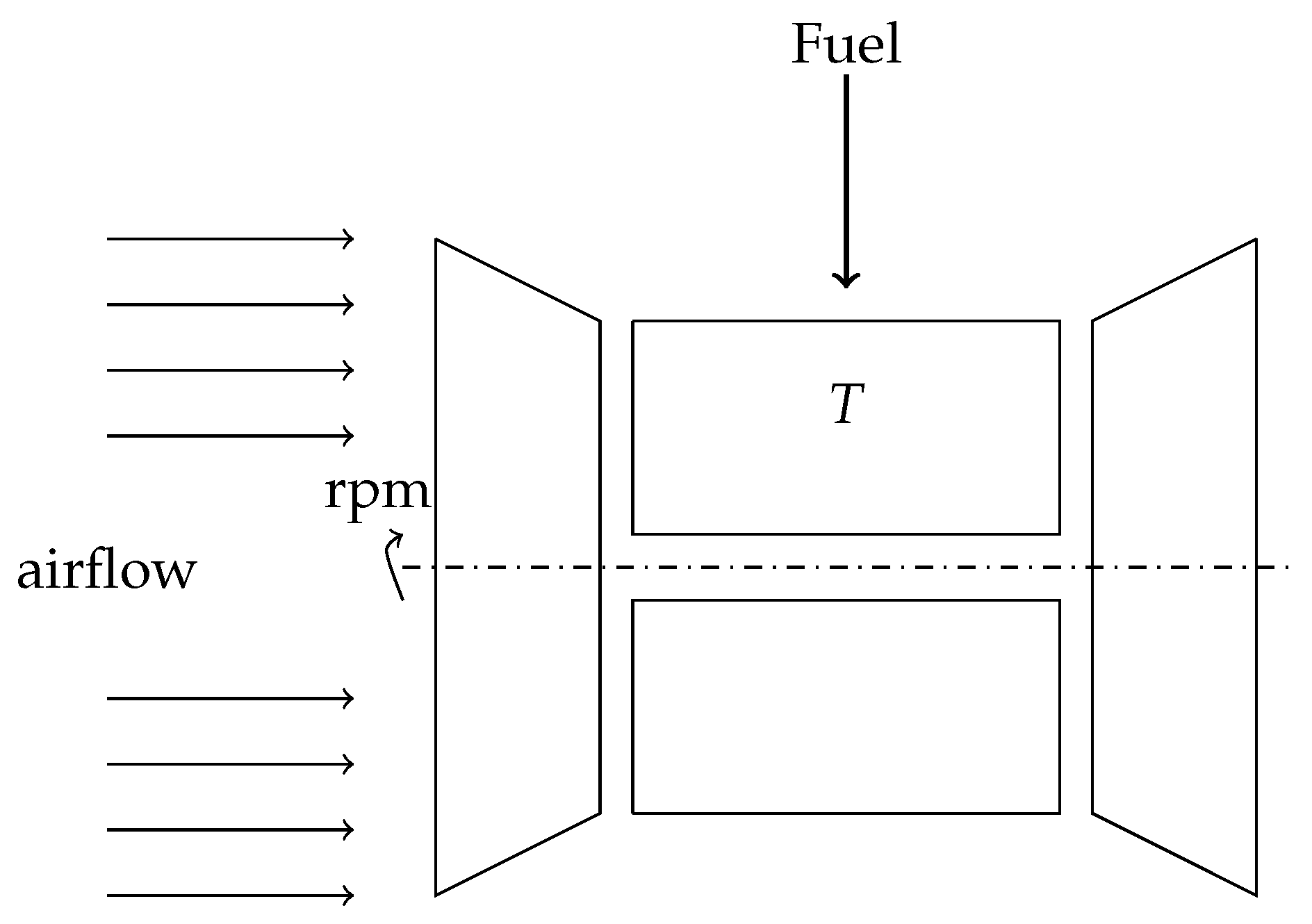
A jet turbine is a well-known engine known for at least 90 years The typical application is that of an aircraft power-plant, but also in some ground applications. The main examples are firefighting and snow removal. In recent years, some companies have started to develop engines optimized for thermal power rather than thrust.
In a very simplistic view (see Figure 2), an already running turbine has one input parameter that is fuel flow. As outputs, we have its rotational speed (given in rpm—r) and temperature (in C—T). In ideal conditions, there should exist a simple relationship between T and r. Since many factors vary and not all of them can be directly measured then we can think about this relationship as probability, which puts us in the framework of the problem stated in the introduction.
7.2. Data Preparation
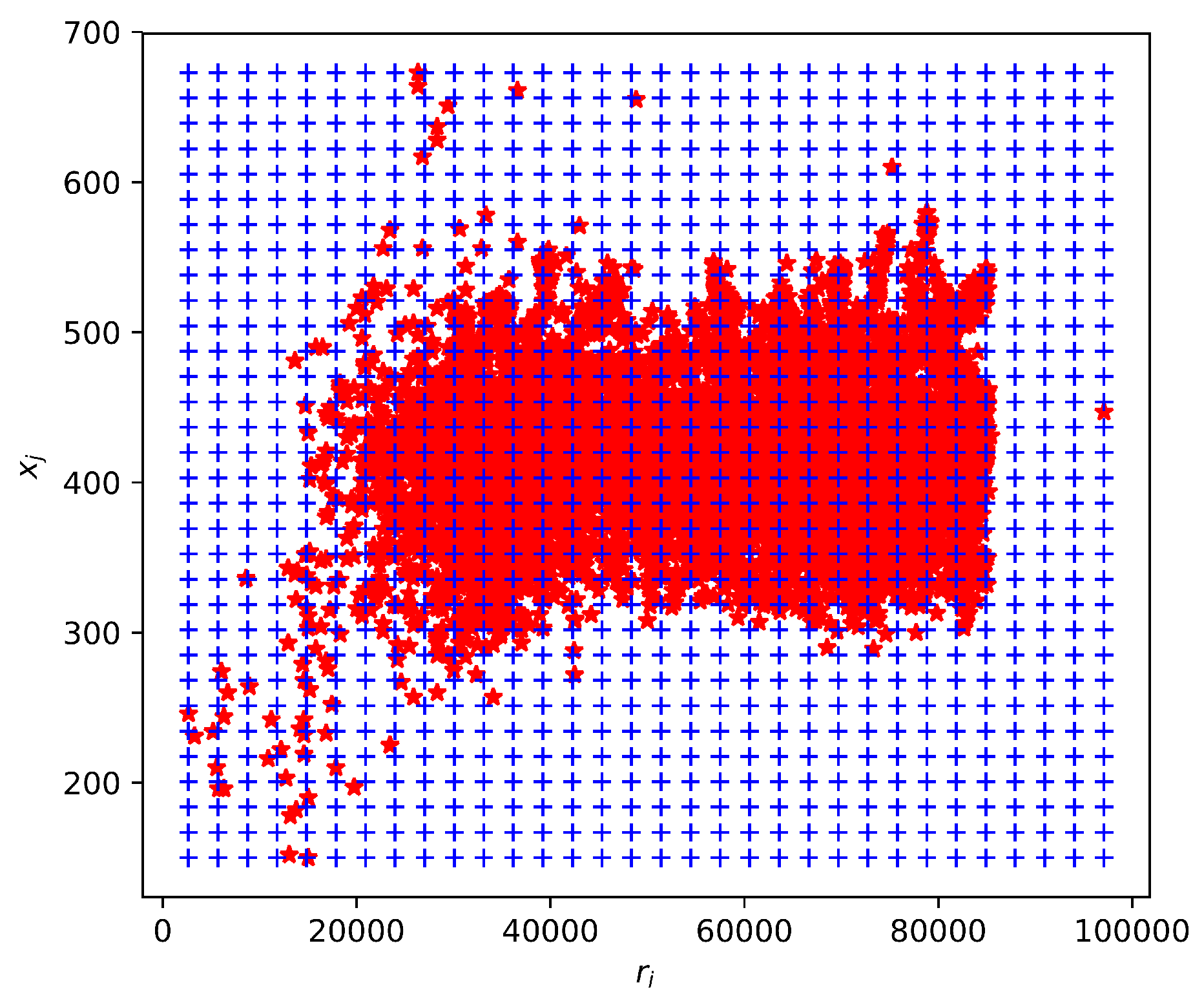
The orginal process data from the server have a form of JSON file of a database table. In this table, we are interested only in two columns, namely the turbine rotation speed (in rpm) and the turbine temperatue. Since the resulting temperature is dependent on many other factors, not all of them measured or even known, we treat the value as a random variable X and the rotation speed as known (so not random) r. The amount of relevant data are 71,268.
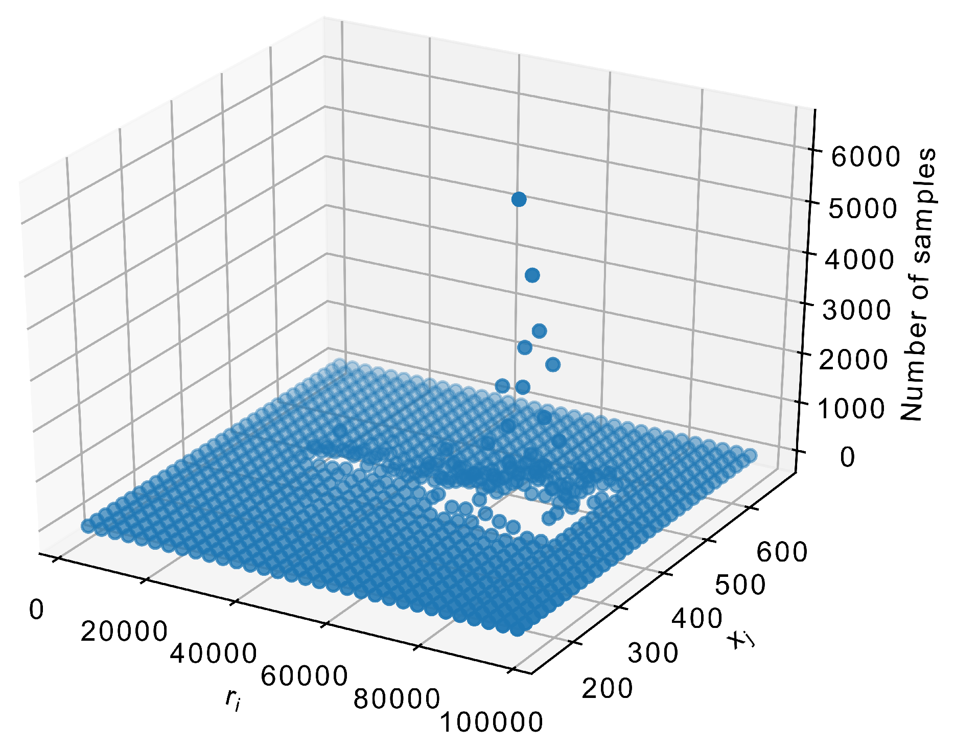
These two columns have to be changed into frequencies for each . Groups are formed on a rectangular grid. An example of such a grid can be seen in Figure 3. The resulting number of samples in each box of the grid is shown in Figure 4. They should be converted into frequencies by simple divison. In order not to obscure the image, a 32 × 32 grid was used.
As a result, we obtain a matrix containing the observations near points on the grid
7.3. The Estimation Process
From the matrix obtained in the previous section, a two-dimensional Discrete Fourier Transform is calculated using the FFT algorithm. The result is a matrix of equal size but containing complex values. In literature regarding the Fourier transform, many properties can be found. A good example is book [22]. We use symmetry and antisymmetry of the resulting matrix. General inversion of the Fourier transform is defined in the following way:
where .
Equation (49) is defined only for the original points of the matrix (48). The continuous surface can be obtained by changing the therms into . We cannot guarantee that between grid points the result would be real. The sensible solution is to use the absolute value of a possibly complex number.
We can ask the question of why use the FFT, if we reconstruct the same data again. The reason is smoothing the result. The reconstruction can use only a selected part of the spectrum—obviously lower frequencies. As mentioned before, they reside in the center of the matrix:
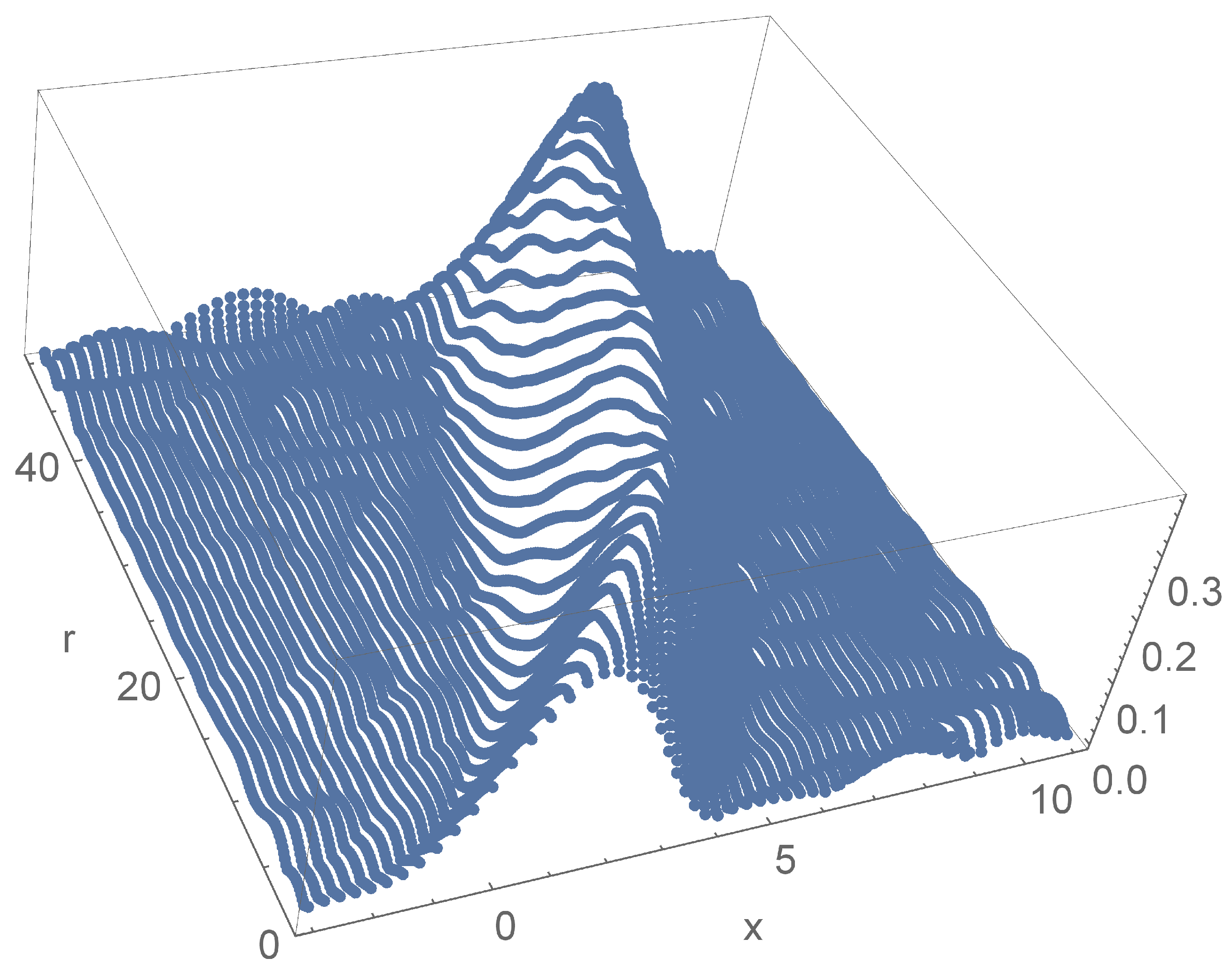
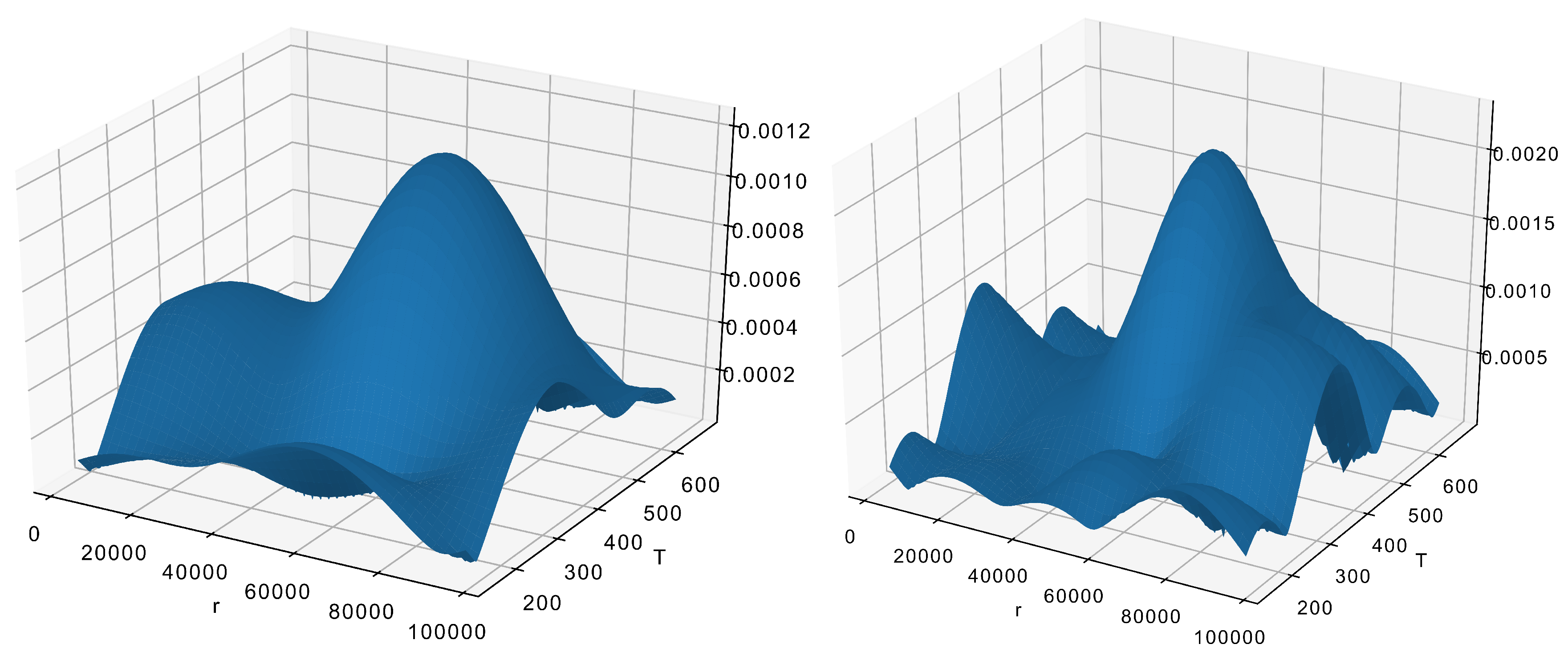
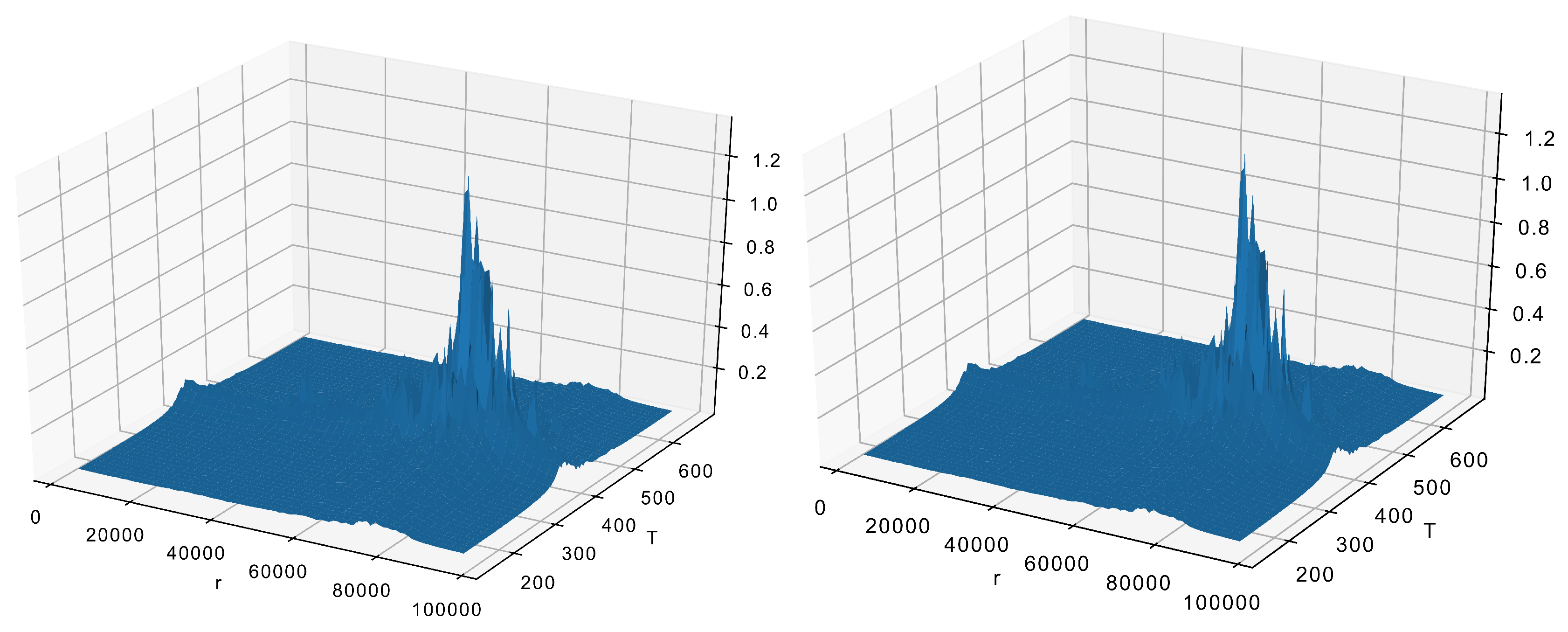
where is the correction factor necessary for compensating for the omitted data. Its values should be selected so the reconstruction result is still p.d.f. and integrates to 1. Obviously, the size of part of the FFT matrix taken is , the careful selection of is crucial. When those numbers are too small (see Figure 5), the result loses any resemblance to the original data (Figure 4). On the other hand, when the numbers are too large, this gives a detailed reconstruction (Figure 6) with all unnecessary details.
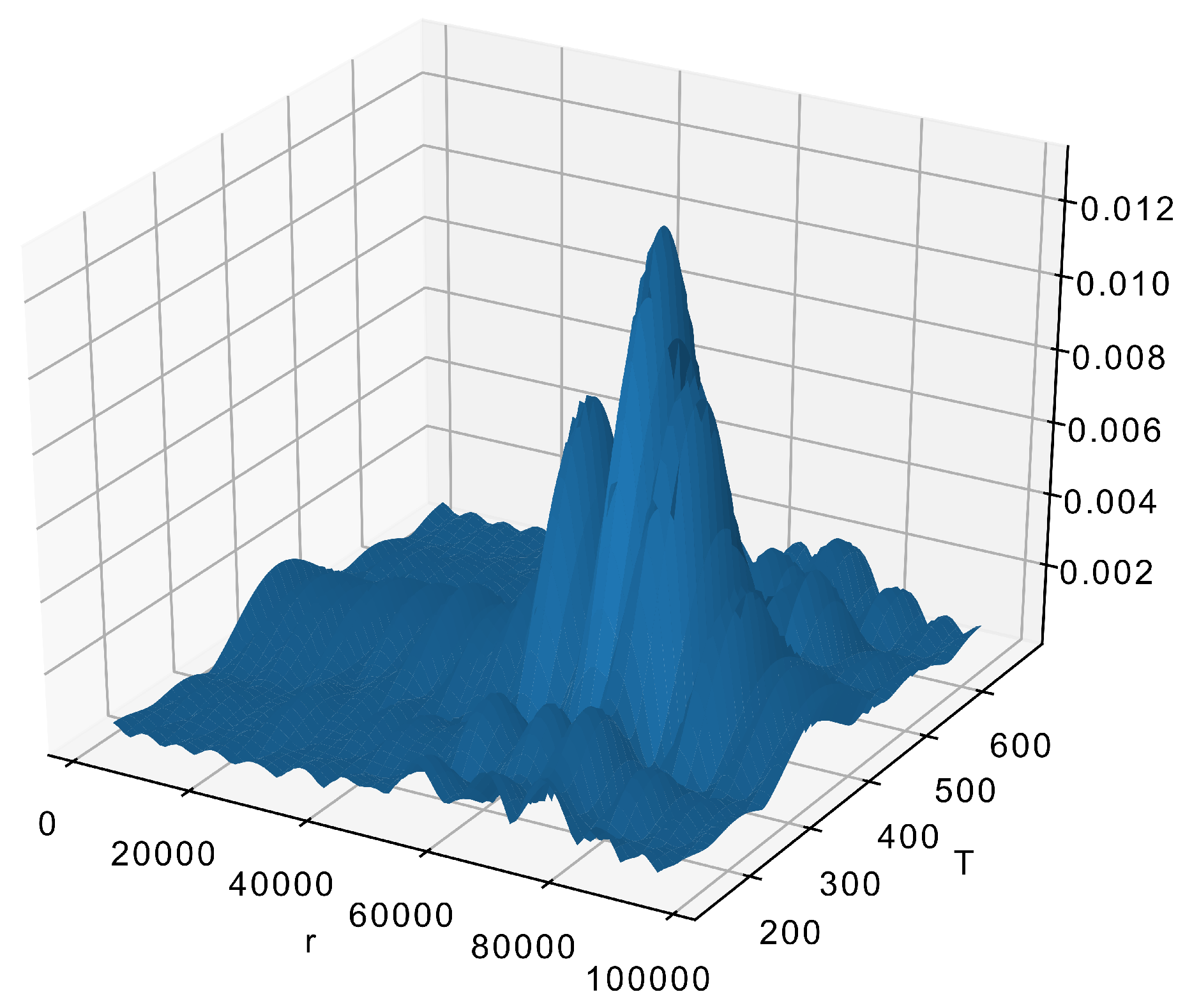
The acceptable reconstruction in Figure 7 is made with and . It is obvious that smaller size means faster calculations.
The exact values can be obtained experimentally (as in this example) or by using some method like the Kronmal–Tarter rule.
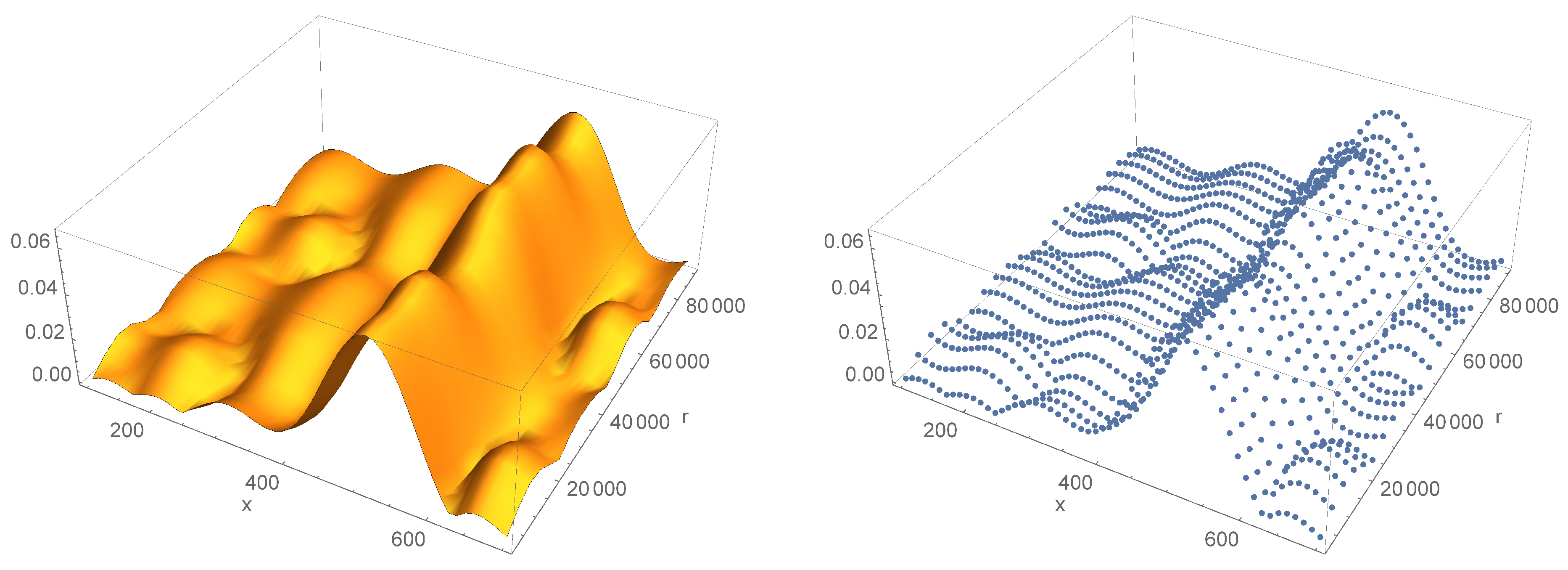
Another heuristic approach is to reduce the abount of the entry points (probabilities) by removing perimeter data. The result of such an approach can be seen in Figure 8. The removal of peripherial data results in reduction of over-fitting.
8. Possible Applications
8.1. Process Simulation
The simulation is an important tool in both design and then subsequent maintenance of the system, especially if physical device is cumbersome, costly, or dangerous to use. The obvious method of simulating the engine temperature at specific rotational speed is to generate random numbers from a distribution specific for that temperature. The simplest method is the so-called acceptance-rejection method. In this method, a random number from distribution is generated as follows (in general using any dense random number generator, but typically uniform is used):
- generate random ,
- generate ,
- if then go to 1, otherwise the result is x.
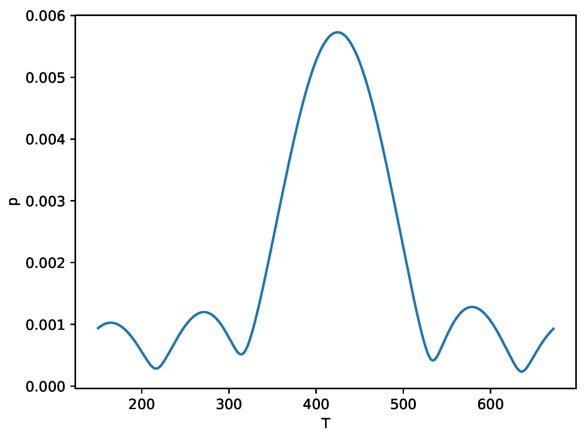
We can easily obtain distribution for a specific parameter r. Using the example from Section 7.1, with r = 50,000 we obtain a distribution as in Figure 9.
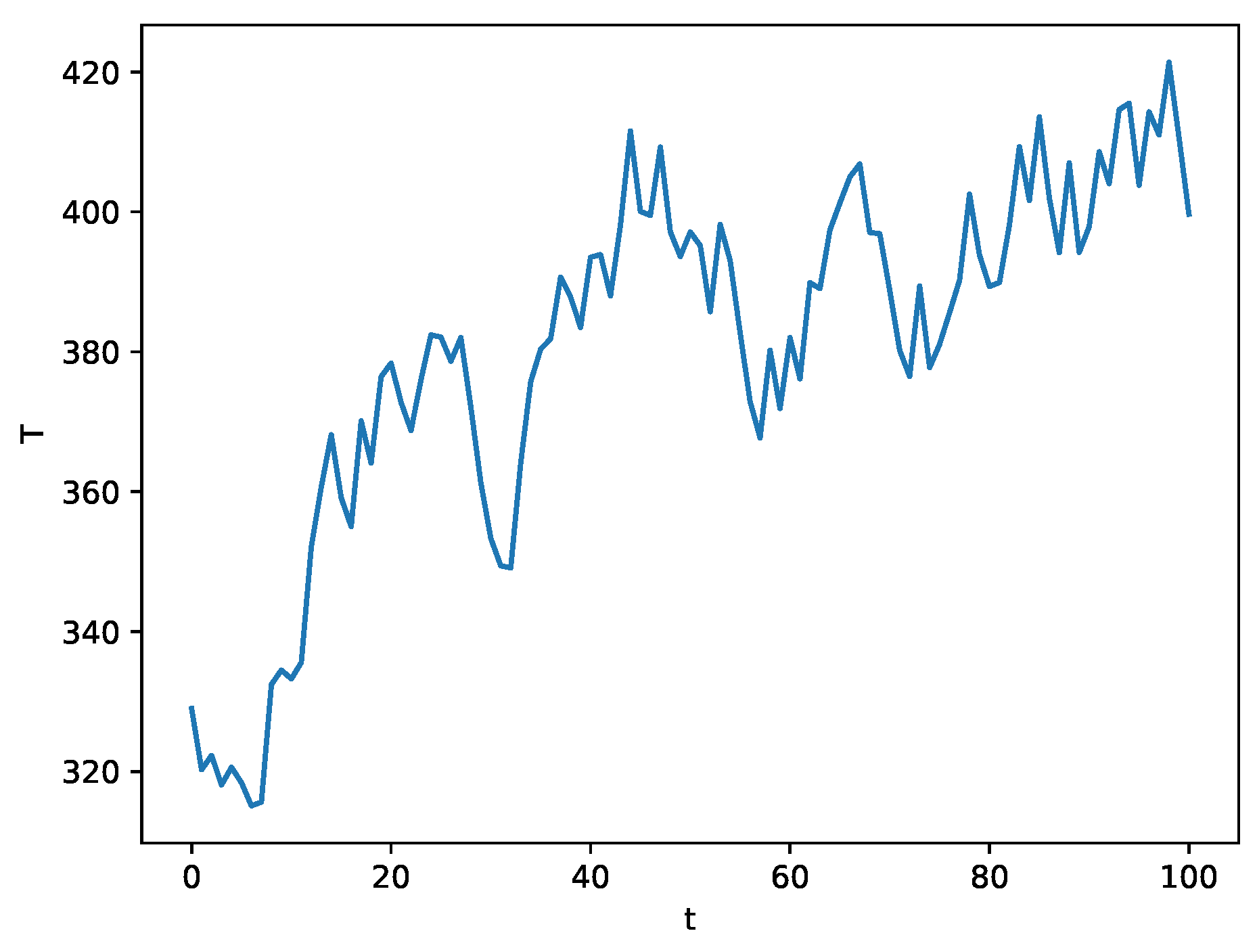
If a random generation algorithm is used directly, the resulting process path would be highly irregular and perceived as not real. To avoid this, a simple filter can be used
where is the resulting new random number, is the new process value, and is the old process value. The result with parameter can be seen in Figure 10.
8.2. Process Diagnostics
From the resulting function , for specific r, we can calculate expected the value of and also some specified interval where of realizations can be found—the equivalent of a confidence interval. If this parameter is selected carefully, we can discern whether the actual pair form the process in or outside it. Other similar diagnostic methods can be seen in [23,24].
9. Convergence of the Learning Procedure
In this section, we prove the convergence of the learning procedure in a simplified version similar to that described in Section 2.2, but without the discretization with respect to r. Then, we shall discuss additional conditions for the convergence of its discretized version.
Let be independent, identically distributed random variables with parameter r, with p.d.f. , where—for simplicity—we assume that n is the same for each r. Then, f has the representation
which is convergent in the norm, where
Then, we estimate ’s as follows:
Lemma 4.
For every is the unbiased estimator of .
Proof.
Indeed,
□
As an estimator of , we take the truncated version of (52):
where the truncation point K depends on n. It may also depend on r, but, for the asymptotic analysis, we take this simpler version.
The standard way of assessing the distance between f and its estimator is the mean integrated squared error (). Notice, however, that, in our case, the MISE additionally depends on r, which is further denoted as . Thus, in order to have a global error, we consider the integrated , which is defined as follows:
The is defined as follows:
where the expectation w.r.t. concerns all ’s that are present in (56).
Using the orthonormality of ’s, we obtain:
Continuing (59), we obtain for each :
It is known that that for squared integrable f we have: . Thus, if when , then for every , we obtain:
This result is not sufficient to prove the convergence of to zero as . To this end, we need a stronger result, namely an upper bound on , which is independent of r.
Lemma 5.
Let us assume that exists and it is a continuous function of x in for each . Furthermore, there exists constant , which does not depend on r, and such that
If when , then—for n sufficiently large, we have:
Proof.
It is known that
Thus, , which finishes the proof, since it is known that for sufficiently large we have . □
For evaluating the variance component, we use Lemma 1:
where is the variance of a r.v. having the p.d.f. .
Let us assume that the orthonormal and complete system ’s is uniformly bounded, i.e., there exists p being a nonnegative integer and such that
Notice that (66) holds for the trigonometric system with
Lemma 6.
Notice that the bound in (67) does not depend on r.
Theorem 2.
Let the assumptions of Lemmas 5 and 6 hold. If the sequence is selected in such a way that the following conditions hold:
then the estimation error as .
Proof.
By Lemmas 2 and 6, we have uniform (in r) bounds for the variance and for the squared bias, respectively. Thus,
Hence,
which finishes the proof by applying (69). □
Observe that for ’s being the trigonometric system we have and the r.h.s. of (71) is, roughly, of the form: , , , which is minimized by for a certain constant . This implies that . Notice that this rate is known (see [25]) to be the best possible when a bivariate, continuously differentiable regression function is estimated by any nonparametric method.
However, this convergence rate was obtained under an idealized assumption that we have observations of ’s for each r. Further discussion of this topic is outside the scope of this paper. We only mention that in [17] it was proved that orthogonal series estimators of p.d.f.’s retain consistency under mild assumptions concerning grouped observations. In particular, in the notation of Section 3, bin width should depend on the number of observations d as follows: as , but in such a way that multiplied by the qube power of the number of spanning orthogonal terms should also approach zero. One can expect that, for the trigonometric series, should also fulfill similar conditions.
10. Conclusions
In this paper, a method for the estimation of families of density functions is presented along with an efficient learning algorithm. It gives insight into the relation between probability density function and external factors that influence it. The method was used in a real-world problem to simulate and diagnose a jet turbine.
Additional, significant possible applications include the estimation of quality indexes for decision-making and optimal control, especially for repetitive and/or spatially distributed processes (see [26,27] for most recent contributions).
From the formal point of view, the method presented can easily be extended into a multidimensional case. Namely, if r is multivariate , say, then it suffices to replace orthogonal system , by the tensor product of ’s, i.e., by all possible products of the following form:
where takes all the values in , . As a consequence, one has to replace all the sums over j by the multiple sums over ’s. When ’s form the trigonometric system, then one can apply the multidimensional algorithm. Clearly, a much larger number of observations is also necessary for a reliable estimation, but a family of estimated p.d.f.’s provides much more information than a regression function of .
Funding
This research received no external funding.
Acknowledgments
The author expresses his thanks to the anonymous reviewers for many helpful comments clarifying the presentation.
Conflicts of Interest
The authors declare no conflict of interest.
References
- Cencov, N.N. Evaluation of an unknown distribution density from observations. Sov. Math. Dokl. 1962, 3, 1559–1562. [Google Scholar]
- Devroye, L. On the almost everywhere convergence of nonparametric regression function estimates. Ann. Stat. 1981, 9, 1310–1319. [Google Scholar] [CrossRef]
- Györfi, L.; Kohler, M.; Krzyzak, A.; Walk, H. A Distribution-Free Theory of Nonparametric Regression; Springer Science & Business Media: New York, NY, USA; Berlin/Heidelberg, Germany, 2006. [Google Scholar]
- Parzen, E. Nonparametric statistical data modeling. J. Am. Stat. Assoc. 1979, 74, 105–121. [Google Scholar] [CrossRef]
- Greblicki, W.; Danuta, R.; Rutkowski, L. An orthogonal series estimate of time-varying regression. Ann. Inst. Stat. Math. 1983, 35, 215–228. [Google Scholar] [CrossRef]
- Rutkowski, L. Application of multiple Fourier series to identification of multivariable non-stationary systems. Int. J. Syst. Sci. 1989, 20, 1993–2002. [Google Scholar] [CrossRef]
- Rutkowski, L. Real-time identification of time-varying systems by non-parametric algorithms based on Parzen kernels. Int. J. Syst. Sci. 1985, 16, 1123–1130. [Google Scholar] [CrossRef]
- Duda, P.; Rutkowski, L.; Jaworski, M.; Rutkowska, D. On the Parzen kernel-based probability density function learning procedures over time-varying streaming data with applications to pattern classification. IEEE Trans. Cybern. 2020, 50, 1683–1696. [Google Scholar] [CrossRef]
- Duda, P.; Jaworski, M.; Rutkowski, L. Convergent time-varying regression models for data streams: Tracking concept drift by the recursive Parzen-based generalized regression neural networks. Int. J. Neural Syst. 2018, 28, 1750048. [Google Scholar] [CrossRef] [PubMed]
- Jaworski, M. Regression function and noise variance tracking methods for data streams with concept drift. Int. J. Appl. Math. Comput. Sci. 2018, 28, 559–567. [Google Scholar] [CrossRef] [Green Version]
- Marron, J.S. A comparison of cross-validation techniques in density estimation. Ann. Stat. 1987, 152–162. [Google Scholar] [CrossRef]
- Bleuez, J.; Bosq, D. Conditions necessaires et suffisantes de convergence de l’estimateur de la densitepar la methode des fonctions orthogonales. Rev. Roum. Math. Pures Appl. 1979, 24, 869–886. [Google Scholar]
- Devroye, L.; Györfi, L. Nonparametric Density Estimation: The L1 View; Wiley: New York, NY, USA, 1985. [Google Scholar]
- Hall, P. On the rate of convergence of orthogonal series density estimators. J. R. Stat. Soc. 1986, B48, 115–122. [Google Scholar] [CrossRef]
- Tarter, M.E.; Kronmal, R.A. An introduction to the implementation and theory of nonparametric density estimation. Am. Stat. 1976, 30, 105–112. [Google Scholar]
- Hall, P. The influence of rounding errors on some nonparametric estimators of a density and its derivatives. SIAM J. Appl. Math. 1982, 42, 390–399. [Google Scholar] [CrossRef]
- Rafajłowicz, E. Consistency of Orthogoal Series Density Estimators Based on Grouped Observations. IEEE Trans. Inf. Theory 1997, 10, 283–285. [Google Scholar]
- Rafajłowicz, E. Nonparametric orthogonal series estimators of regression: A class attaining the optimal convergence rate in L2. Stat. Probab. Lett. 1987, 5, 219–224. [Google Scholar] [CrossRef]
- Rafajłowicz, E.; Skubalska-Rafajłowicz, E. FFT in calculation nonparameteric regression estimate based on trigonometric series. Appl. Math. Comput. Sci. 1993, 3, 713–720. [Google Scholar]
- Hall, P.; Marron, J.S. Extent to which least-squares cross-validation minimises integrated square error in nonparametric density estimation. Probab. Theory Relat. Fields 1987, 74, 567–581. [Google Scholar] [CrossRef]
- Kronmal, R.; Tarter, M. The estimation of probability densities and cumulatives by Fourier series methods. J. Am. Stat. Assoc. 1968, 63, 925–952. [Google Scholar]
- Rao, K.; Kim, D.; Hwang, J. Fast Fourier Transform-Algorithms and Applications; Springer Science & Business Media: Dordrecht, The Netherlands; Heidelberg, Germany; London, UK; New York, NY, USA, 2011. [Google Scholar]
- Gałkowski, T.; Krzyżak, A.; Filutowicz, Z. A New Approach to Detection of Changes in Multidimensional Patterns. J. Artif. Intell. Soft Comput. Res. 2020, 10, 125–136. [Google Scholar] [CrossRef]
- Skubalska-Rafajłowicz, E. Random projections and Hotelling’s T2 statistics for change detection in high-dimensional data streams. Int. J. Appl. Math. Comput. Sci. 2013, 23, 447–461. [Google Scholar] [CrossRef] [Green Version]
- Stone, C.J. Optimal global rates of convergence for nonparametric regression. Ann. Stat. 1982, 1040–1053. [Google Scholar] [CrossRef]
- Mandra, S.; Galkowski, K.; Rauh, A.; Aschemann, H.; Rogers, E. Iterative Learning Control for a Class of Multivariable Distributed Systems With Experimental Validation. IEEE Trans. Control Syst. Technol. 2020. [Google Scholar] [CrossRef]
- Rafajłowicz, W.; Więckowski, J.; Moczko, P.; Rafajłowicz, E. Iterative learning from suppressing vibrations in construction machinery using magnetorheological dampers. Autom. Constr. 2020, 119, 103326. [Google Scholar] [CrossRef]
Figure 1.
A result for the synthetic problem.

Figure 2.
Simplified schematics of turbine—parts important for current investigations.

Figure 3.
Data and 32 × 32 grid for frequencies.

Figure 4.
Number of samples in the grid (reduced to 32 × 32 for display’s sake).

Figure 5.
Insufficient amount of Fourier-transformed data, the result is too smooth (2 × 2 in the left, 4 × 4 in the right).
Figure 5.
Insufficient amount of Fourier-transformed data, the result is too smooth (2 × 2 in the left, 4 × 4 in the right).

Figure 6.
Use of too much Fourier-transformed data (64 × 64 in the left) and full reconstruction (right).
Figure 6.
Use of too much Fourier-transformed data (64 × 64 in the left) and full reconstruction (right).

Figure 7.
Good selection of data for smoothing, 16 in r, 4 in T.

Figure 8.
Reduction of the primeter data in order to avoid over-fitting. Left: reconstruction based on partial data, Right: resulting points.
Figure 8.
Reduction of the primeter data in order to avoid over-fitting. Left: reconstruction based on partial data, Right: resulting points.

Figure 9.
Probability for 50k rpm.

Figure 10.
A result of smoothed simulation for 50k rpm.


Table 1.
Result of distance calculation between synthetic data and reconstruction.
| Method | Mean | Standard Deviation |
|---|---|---|
| Hellinger | 0.00007 | |
| Kullback–Leibler | 0.00014 |
© 2020 by the author. Licensee MDPI, Basel, Switzerland. This article is an open access article distributed under the terms and conditions of the Creative Commons Attribution (CC BY) license (http://creativecommons.org/licenses/by/4.0/).
Share and Cite
MDPI and ACS Style
Rafajłowicz, W. Nonparametric Estimation of Continuously Parametrized Families of Probability Density Functions—Computational Aspects. Algorithms 2020, 13, 164. https://0-doi-org.brum.beds.ac.uk/10.3390/a13070164
AMA Style
Rafajłowicz W. Nonparametric Estimation of Continuously Parametrized Families of Probability Density Functions—Computational Aspects. Algorithms. 2020; 13(7):164. https://0-doi-org.brum.beds.ac.uk/10.3390/a13070164
Chicago/Turabian StyleRafajłowicz, Wojciech. 2020. "Nonparametric Estimation of Continuously Parametrized Families of Probability Density Functions—Computational Aspects" Algorithms 13, no. 7: 164. https://0-doi-org.brum.beds.ac.uk/10.3390/a13070164
Note that from the first issue of 2016, this journal uses article numbers instead of page numbers. See further details here.