Sliding Mode Control Algorithms for Anti-Lock Braking Systems with Performance Comparisons


Department of Automation and Applied Informatics, Politehnica University of Timisoara, Bd. V. Parvan 2, 300223 Timisoara, Romania
*
Author to whom correspondence should be addressed.
Algorithms 2021, 14(1), 2; https://0-doi-org.brum.beds.ac.uk/10.3390/a14010002
Submission received: 26 October 2020
/
Revised: 7 December 2020
/
Accepted: 21 December 2020
/
Published: 23 December 2020
(This article belongs to the Special Issue 2020 Selected Papers from Algorithms Editorial Board Members)
Abstract
:This paper presents the performance of two sliding mode control algorithms, based on the Lyapunov-based sliding mode controller (LSMC) and reaching-law-based sliding mode controller (RSMC), with their novel variants designed and applied to the anti-lock braking system (ABS), which is known to be a strongly nonlinear system. The goal is to prove their superior performance over existing control approaches, in the sense that the LSMC and RSMC do not bring additional computational complexity, as they rely on a reduced number of tuning parameters. The performance of LSMC and RSMC solves the uncertainty in the process model which comes from unmodeled dynamics and a simplification of the actuator dynamics, leading to a reduced second order process. The contribution adds complete design details and stability analysis is provided. Additionally, performance comparisons with several adaptive, neural networks-based and model-free sliding mode control algorithms reveal the robustness of the proposed LSMC and RSMC controllers, in spite of the reduced number of tuning parameters. The robustness and reduced computational burden of the controllers validated on the real-world complex ABS make it an attractive solution for practical industrial implementations.
1. Introduction
The anti-lock braking system (ABS) is a mandatory safety feature in modern vehicles [1] and constitutes an attractive benchmark for control applications. One of the common approaches that has been studied for ABS control is the so-called slip-control. It is well-known that when braking or accelerating, a traction force owed to the friction appears at the contact surface between the tire and the road [2,3]. This force amplitude proportionally depends on the normal force at the contact point. A friction coefficient called is representative for the traction behavior, it is surface dependent and well-acknowledged research showed that this friction coefficient is a function of the wheel slip coefficient denoted [4].
In principle, the associated control problem is to impose a desired value for the wheel slip , that is, to set at a desired value for the relative difference between the wheel velocity and the road (or car) velocity [2,5]. This problem is known as slip control. Among all implemented braking approaches, the slip coefficient control is arguably the most intensively studied in many theoretical and practical implementations [6].
Historically, the wheel lock prevention concept under braking was conceived almost a century ago in the mid-1930s by Robert Bosch’s patents [7,8,9] and was technically implemented at the end of the 60s when inductive contactless sensors replaced the mechanical ones [9]. The strong electronics development led to powerful integration and robust operation; therefore, hydraulic pressure regulation became possible based on data gathered from the sensors mounted in the proximity of the wheel ensemble. ABSs for serial production became available starting in 1978 [9,10]. The focus has shifted since then towards assuring more intelligent control algorithms for the ABS, reviews of such approaches can be checked with earlier works of [11,12] and more recently with [13,14,15,16].
Slip control is a difficult task for a number of reasons:
- -
- The ABS dynamics in braking mode are extremely nonlinear and many parameters of the underlying model change with time.
- -
Among the existing control techniques, sliding mode control (SMC) is an already vastly studied and mature methodology that, among many other control approaches, has proved its success in many industrial applications due to its simplicity and robustness [19,20,21,22,23]. It has also been applied before to ABS slip control systems in combination with different controllers or just as standalone as presented next, however, without the detailed performance assessment through comparisons with different control methods.
An SMC design can be traced back to the work of Drakunov et al. [11], where a detailed hydraulic actuator model is provided and a friction force observer adds computational complexity to the design. However, an extremum searching algorithm was devised for the optimal slip reference input that maximizes the braking friction force (by maximizing the friction coefficient ). An underlying PID-based slip control was employed in [12] where a sliding-mode optimizer is used for computing the optimal slip reference input but does not benefit from the SMC in the closed-loop. Unsal and Kachroo [3] proposed a nonlinear observer SMC-based slip controller combined with computationally demanding sliding observers for vehicle velocity estimation. A self-learning fuzzy sliding-mode control design was proposed by Lin and Hsu [18], where the tuning algorithm of the controller is derived in the Lyapunov sense, but the braking model is a very simplified one. A linearization-based SMC law was proposed in [23] on a simplified quarter-car ABS model without accounting for actuator dynamics. While a similar simplified braking model was employed with a recurrent neural network (RNN)-based uncertainty observer, in a hybrid SMC design provided by [24]. Noticing that the adaptive laws of the RNN bring supplementary computational burden rather than account for uncertainties by typical upper bounds. A comprehensive experimental validation on a braking system of a real-life scale laboratory car was proposed by [25]. Although a very detailed model is provided, uncertainty is not accounted for in the SMC design, and with the experimental validation as the main focus, the theoretical stability analysis is missing. Another quasi-SMC ABS controller with endocrine neural network-based estimator was presented in [26]. In order to increase the steady-state accuracy, the estimated modeling error is included in the controller at the cost of computational complexity. A simpler SMC design with included model uncertainties and integral switching surface for chattering reduction was suggested in the work of [17] on a four-wheel car model with simplified dynamics. However, theoretical stability certificates were not provided in the mentioned work. Other control approaches for ABS include nonlinear adaptive solutions [5,10], data-based approach [1], fractional SMC [4], fuzzy [16] and neuro-fuzzy sliding mode incremental learning [27] and grey system modeling approach for SMC [28]. More recent application-oriented validation of intelligent ABS control is presented in the works [29,30,31,32].
The contribution of this work is threefold. Firstly, the original SMC laws (LSMC and RSMC) are proposed and they have not been applied before to ABS control systems. Secondly, their complete design and stability analysis show that the SMC control is robust enough to account for large uncertainty in the design, without additional uncertainty estimator and without striving for complex models, even though the actuator dynamics is simplified to a simple gain. This operation is required in order to bring the ABS model to a second-order system dynamics favorable to the SMC design, herein proposed in two variants. Thirdly, the comparisons with other four competitive controllers also prove the performance capability attainable with such SMC-based controllers. These controllers are of various types: an adaptive one, a model-free reinforcement learning one, a model-free SMC one and a model-based periodic switching sliding-mode controller. Without a significant computational burden and with proven control performance, such sliding-mode controllers are attractive for industrial implementations, owing to their robustness, simplicity and few tuning parameters.
In the following, Section 2 briefly describes the ABS system and the slip regulation control problem, while Section 3 proposes two variants of sliding mode control design. Section 4 validates the two approaches and compares the results with a state-of-the-art adaptive approach. Conclusions are highlighted in Section 5.
2. The Anti-Lock Braking System Model
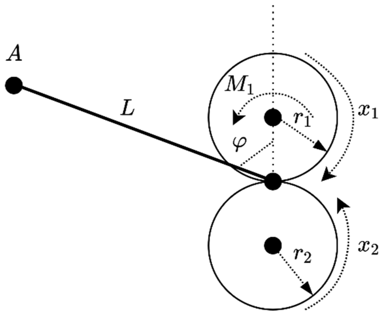
The ABS braking system equipment from [15] (Figure 1) consists of two vertically superimposed wheels that simulate the relative motion between the road (lower wheel) and the quarter-car model (upper wheel). Throughout the braking process, the two wheels remain in contact and interaction occurs at the contact surface between them.
The upper wheel is equipped with a disk braking system actuated by a braking lever, which is itself actuated by an inextensible string tensioned with the help of a pulley attached to a small flat DC motor [15]. The lower wheel is spin by the bigger flat DC motor, which is power-supplied to accelerate the wheel. After the two wheels in contact reach a threshold angular speed, the braking phase starts with the bigger DC motor left in free running mode (no power) while the smaller DC motor actuates the braking mechanism. Both DC motors are electronically controlled by pulse-width modulation (PWM) signals of 3.5 kHz. The varying pulse-width of the upper wheel is the control input variable denoted as u, in the following equations of motion [15,33]:
where the angular speed for the upper wheel is denoted as (measured in rad/s), and for the lower wheel is denoted . The time argument is omitted next for simplified notation. Additionally, in braking mode, and are given constant parameters. M1(t) is the braking torque evolving according to the third differential equation, where constants b1 and b2 model the actuator dead-zone dynamics whose threshold is u0, while depends on the constant angle and is the friction coefficient ()-slip coefficient () static characteristic with being known constants. Notice at this point that the model (1) is not obtained directly, but its coefficients depend on many physical parameters of the ABS system and can be recovered in the original documentation [15]. Some of them are properly presented throughout the paper when needed.
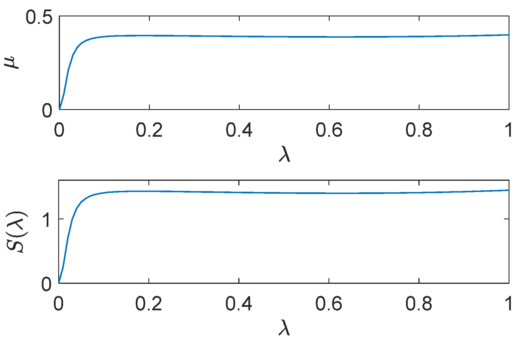
In slip control strategy, the aim is to regulate to the value of corresponding to the peak of the – curve [15]. This implies for maximum friction coefficient, and favorable minimum braking distance and time. In real world commercial braking systems, the weight load on the car, the tire inflation state and wear, the road-tire contact surface and the road surface profile combined with the car speed, all interplay with the braking process and may affect the – curve profile significantly. The static characteristics are shown in Figure 2.
In the braking mode, the slip is defined as:
where r1, r2 are the radii of the two wheels in contact. For the given laboratory model, since the two radii are approximately equal, it will be considered that r1 = r2 = 0.99 [m], leading to a simpler slip in (2), i.e., .
From a functional perspective, there are three torques acting on the upper wheel: the braking torque M1, the friction torque in the upper bearing and the friction torque among the wheels. There are two torques acting on the lower wheel: the friction torque in the lower bearing and the friction torque among the wheels. Besides these, two gravity force of the upper wheel and the pressing force of a shock absorber of the upper wheel force the contact between the two wheels [15].
The values of the ABS model parameters in (1) are [15]: , , , , , , , , , , and depend on the physical parameters of the ABS system. Additionally, the parameters that define are , , , , , , , .
For the subsequent sliding-mode control design, given that the dead-zone in the braking torque dynamics has known parameters and therefore it can be compensated by proper additive component at the control input level, an order reduction of the model (1) is performed. Therefore, it is justified to bring b(u) to a linear dependence of the form on u(t). Then it is apparent that the linearized actuator dynamics holds as the transfer function , with time constant . Neglecting these dynamics leads to with constant , as the simplified actuator dynamics that turns (1) into a second-order state-space model of the form
where
In the following, the sliding mod control design is aimed and presented in two proposed variants.
3. Sliding Mode Control Design
Adoption of sliding mode control algorithms relies on the well-acknowledged robustness of these algorithms to parameter variation and uncertainty. The control problem essentially requires regulation to a given slip value. Should the desired slip be set around the peak of the – curve in Figure 2 (this peak is surface-dependent), some desirable braking behavior takes place, characterized by maximum deceleration, on maximum friction and minimal braking time and distance.
In the following, two variants of sliding mode control strategies for the ABS system are presented and designed in detail. The first sub-section presents the Lyapunov-based sliding mode controller (LSMC) design, followed by the presentation of the reaching law-based sliding mode controller (RSMC) design.
3.1. Lyapunov-Based Sliding Mode Control Design with Included Uncertainties in the Process Model
A convenient artificial construction of a Lyapunov type function is used indirectly in determining a control law that ensures at the same time the stability of the entire control system. The resulting controller is called the LSMC controller in the following.
Let the state-space model of the ABS system be rewritten from (3) as
where v1 and v2 are additive terms accounting for unmodeled dynamics, external disturbances and parametric uncertainties. A switching variable is defined as , with the desired slip. We notice that since the simplified slip in (2) is , then is equivalent to the sliding surface line equation which is consistent with the more familiar definition of the sliding surface in the form .
Let be a Lyapunov function depending on . Then , and furthermore, to ensure the reaching condition of the sliding surface , it is sufficient to have , or, for reaching in finite time it is needed to ensure .
Since the calculation of is needed, the derivative of the slip is found, based on (5) as
where the terms containing the perturbations have been included in a single perturbing term considered bounded by .
Finally, the derivative of the switching variable is
Then, to ensure the reaching condition , the following two cases, each with two subcases are developed as:
Finally, the control law that ensures the fulfillment of the reaching condition in all four subcases is captured by the LSMC control law:
with ensuring a smooth implementation of the mathematical sign function denoted and prevents the division by zero in calculations. ensures conservative fulfilment of the inequalities in the four subcases above [6].
The steps of the LSMC algorithm (Algorithm 1) at the current numerical integration step are given next.
| Algorithm 1. The LSMC Algorithm |
| Selected initial parameters 1. Read the desired slip value and the angular speed values . 2. Calculate from (2), then calculate . Find , from (6), calculate from (7). 3. Calculate from (8) and send it to the process. 4. After the current integration step is finished, go to step 1. |
For an insight into the derivation of the LSMC control law (8), please consult the Appendix A. The stability of the control system under the LSMC control law is next asserted.
Theorem 1.
The ABS system (3), (4) with the LSMC control law (8) is asymptotically stable.
Proof of Theorem 1.
The control law (8) is selected to ensure the reaching condition . By an increased value of , the value of is bounded away from 0 (see also Appendix A). Which in turn ensures that the Lyapunov function over time implying reaching for the sliding surface in finite time.
Besides, on the sliding manifold , the closed-loop dynamics have reduced order, since leads to the control from (8) replaced in (5) and to the simplified dynamics constrained by . The resulted system is a linear first order differential equation in with initial condition , of the form where . The dependence is shown in Figure 3 below for in {0, 0.05, 0.1, …, 1}.
The above differential equation is asymptotically stable for all (Figure 2) where . Then Theorem 4.2 from [34] claimed by Theorem 2.1 from [35] implies asymptotic stability of the closed-loop system, whenever the reduced order system on the sliding surface if asymptotically stable and when the evolution of the closed-loop on the sliding surface is preserved. Consequently, which completes the proof. □
3.2. Reaching Law Sliding Mode Control Design with Partial Process Model Uncertainty
For the non-linear second-order process model (3), the feedback error between the desired slip and the actual one is captured by the following variable:
that also acts as a switching variable for the RSMC design, as seen next. The derivative of the slip variable is:
and by separating the terms of the expression for obtaining an expression affine with respect to the control input, we have:
which simply can be compactly written as:
Let the control law be chosen as:
By replacing the command law from (13) into (12), the dynamic of the switching variable is obtained as in:
Depending on the slip derivative , the two analyzed cases are:
- involves , meaning that is decreasing to zero.
- involves , meaning that is increasing to zero.
The most relevant advantage of the RSMC design is that a finite time of reaching the switching surface is guaranteed, calculated as .
It is unlikely that in practice, the model is a true representation of the reality. Hence, for the subsequent control design, this model is considered as partially uncertain, the true model being of the form in which the assumed bounded uncertainty includes unmodeled dynamics, parametric uncertainties and external disturbances, with an user-selectable upper bound to account for the worst case disturbance scenario. In this case, for the control law having the expression (13), the switching variable dynamic of the true model becomes .
In order to guarantee a finite reaching time in the presence of modeling uncertainties, two cases are again identified:
- The case . For a finite reaching time, it is necessary that , with as a positive constant. In this case, it is necessary that . Since , a value ensures a finite reaching time at most equal to .
- The case . In similar reasoning, a value as ensures which involves that the attainment of the finite reaching time is at most.
The steps of the RSMC algorithm (Algorithm 2) at the current numerical integration step are summarized next.
| Algorithm 2. The RSMC Algorithm |
| Selected initial parameter 1. Read the desired slip value and the angular speed values . 2. Calculate from (2), then calculate . Find from (12). Compute the derivative . 3. Calculate as in (13) then send it to the process. 4. After the current integration step is finished, go to step 1. |
The stability of the control system under the RSMC control law is next asserted.
Theorem 2.
The ABS system (3), (4) with the RSMC control law (13) is asymptotically stable.
Proof of Theorem 2.
Let a Lyapunov function candidate be . We observe that the control law (13) leads to the dynamic of the switching variable being . These dynamics ensures that is negative and bounded away from 0 by a suitable selection of a larger k. Which in turn ensures that over time.
On the sliding manifold , the closed-loop dynamics have reduced order, since leads to the control from (13) substituted in (5) and to the simplified dynamics constrained by . The simplified dynamics lead -after some calculations- to a (family of) linear differential equations in , of the form with . This family of -dependent equations is shown in Figure 4 below for in {0, 0.05, 0.1, …, 1}.
This reduced order system is again asymptotically stable for all where , with since is being bounded below by zero: because of braking, the car must come to a full stop. Then again, Then Theorem 4.2 from [34] claimed by Theorem 2.1 from [35] implies asymptotic stability of the closed-loop system, whenever the reduced order system on the sliding surface if asymptotically stable and when the evolution of the closed-loop on the sliding surface is preserved. Consequently, which completes the proof. □
Comment 1. Both situations related to the implementation of the command in the form (13) suggest choosing a larger value of the parameter k. On the other hand, a larger k value introduces high amplitude switching at the control input level, due to the switch element sgn(g). A compromise is needed: the more accurate the model (2) is, the smaller k parameter value is admitted.
Comment 2. Towards the braking process’ end, the lower wheel speed tends to zero. To ensure good numerical conditioning, the denominator occurring in both in (12) and in both in (6), is replaced with , where is a small positive number. In practice this is less problematic since, at low car speeds, it is common to deactivate the ABS control.
Comment 3. The sign function of the control law (13) is practically implemented using the modified sign function defined in (8).
Comment 4. For the computed control laws (8) and (13) to avoid deep control input saturation that could lead to significant windup followed by high-amplitude oscillations, the control inputs calculated as in (8) and as in (13) are manually saturated inside [–1;1] (also observing that the control input domain is not actually usable from the viewpoint of the DC motor actuator, but it is preserved to further show that the SMC compute the actual control inputs in this domains also). On the other hand, this saturation could restrict the domain of the sliding manifold and lead to a longer reaching phase.
4. Validation Case Study
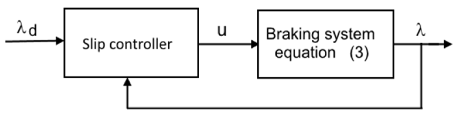
The sliding-mode control algorithms LSMC and RSMC (from Algorithms 1 and 2, respectively) are next validated on the slip control for the ABS process that was introduced in the second Section. First, the controllers’ parameters are experimentally tuned to their best values who attain the smallest performance index on a given test scenario. Towards the section’s end, a systematic optimization-based tuning is employed, to challenge the best achievable control performance from the LSMC and the RSMC. The feedback slip control system is presented in Figure 5.
For subsequent comparisons, the following test scenario for all the controllers uses a desired slip calculated as a step input with amplitude 0.15 that is filtered through the first order lag transfer function . This way, the controlled slip should track the output of a linear output reference model. The angular speed of the wheels at the start of the braking cycle is 180 rad/s. This angular speed is usually obtained after accelerating the two wheels in contact through the lower wheel. The continuous-time controller equations are numerically integrated using a fifth order solver with the fixed step size of 10–3 seconds (s), which is consistent with the real-world execution times. The sampling time corresponding to the fixed step solver allows for data acquisition in order to collect the discrete-time values of as , respectively. Which in turn allows the computation of the following performance index
where ki is the sampling instant index corresponding to the start of the braking process, and N samples of the controlled slip and desired slip are measured, until the angular speed x2 of the lower wheel (the “car”) drops below 10 rad/s towards the end of the braking cycle.
The experimental parameter values for the LSMC control law (8) are selected as . And the parameters of the RSMC law (13) are selected as . Notice that for the RSMC needs not to be estimated since it can be accounted for, by the selection of a large enough .
Several additional controllers are next used to benchmark the performance of the LSMC and RSMC structures. We choose the first adaptive active dynamic controller (ADC) since it is a recent one implemented on the same ABS system, obeying the same working principles as our system. In fact, the ABS system is from the same manufacturer. The second reinforcement learning (RL) model-free controller stems from a different paradigm that does not use the system dynamics, therefore it is designed to cope with significant amount of uncertainty, as it is the case with RSMC and LSMC. This controller was originally proposed, developed and validated on the same ABS system. The third model-free sliding-mode controller combines the feature of the second reinforcement learning controller (in the sense that it is model-free and it does not use the system dynamics knowledge) and also the working principle of sliding-mode control (SMC). Therefore, it fits the comparisons goal. The fourth periodic switching sliding mode controller (PSSMC) is added for comparisons since it is designed to deal with uncertainties under output feedback only with no full state measurement and has been applied to a simplified ABS model before.
(1) An adaptive active dynamic controller (ADC) is also implemented according to the laws presented in [36], that is
where the control design parameters are selected as in [36], the constant parameters specific to the ABS system are corresponding to the inertial moments of the upper and lower wheels, respectively, and measured in [kg m2], the viscous frictions are measured in [kg m2/s], the static frictions in the upper and lower wheel are in [Nm]. The terms are used to approximate the original term related to the normal force Fn from the original ABS equations [1], with the so-called Pacejka’s magic formula, for the parameter’s values .
A notable observation is that the control law (16) is directly expressed in the braking torque M1, thus neglecting the actuator dynamics. To make the controller (16) compatible with controllers (8) and (13), M1 is transformed back into control input u by using the simplified actuator model, that is . To be consistent with the control inputs calculated by the LSMC and RSMC laws (8) and (13), respectively, the braking torque is further saturated to [–9;9] after being calculated from (16).
(2) A reinforcement learning model-free controller. Another controller used for comparisons is a neural network (NN)-based one that was learned under model-free (unknown dynamics) principle using reinforcement Q-learning. As presented in the third case study of the work [33], the reinforcement learning controller (further referred to as simply RL) is a feed-forward NN with 6 inputs, two hidden layers, each having ten neurons with hyperbolic tangent activation function and one output layer having one neuron with linear activation.
This NN controller’s input is a virtual state built from: the current sample values of the two wheels’ speeds and their previous sample values, the previous control input and the current sample desired slip. The previous sample values account for the un-measurable state of the actuator to ensure that the reinforcement Q-learning deals with a fully observable Markov decision process.
Although the controller was learned from transition samples collected in discrete-time by interacting with the process under the conditions presented in [33], this discrete-time is made compatible with the fixed time step-size of the continuous-time SMC controllers. The RL controller learned to brake for various initial speeds and for various slip set points. An additional NN was used (called the Q-function NN) to store the state-action cost function. From a functional perspective, the RL controller is a state-feedback one—it uses separately and not compacted in the slip equation—as opposed to the output-feedback SMC-based ones and to the output-feedback ADC one who use directly.
The learning was performed in an episodic style: each braking scenario starting from a non-zero speed under the current episode controller generates input-output transition samples that were used to build a virtual state of past input-output samples. The batch of transition samples were added to enrich a database that grows with each braking episode. After each episode, the Q-function estimate is improved (in fact, a Q-NN was trained towards the optimal Q-function) and the current episode controller is improved towards the optimal controller. The objective was to minimize an infinite-horizon but discounted version of the performance index , which makes the tuning objective approximately minimize . For additional details please consult [33].
(3) A model-free sliding-mode controller (MFSMC). In the work of [37], two model-free sliding mode control system structures were proposed, the second one proposes the control law:
where is the tracking error with respect to the target slip and is the uncertainty estimate stemming from a first order phenomenological model simplification of the ABS system that reads . Here, is a user-selectable constant parameter seen as a minimal process knowledge, are the user-selectable parameters of the intelligent PI (iPI) controller part, is a switching variable defined in terms of , the user-selectable imposes the desired behavior on the sliding surface . Additionally, acts as another design parameter as the upper bound of the uncertain tracking error dynamics and is again user-selectable to ensure a conservative stability condition. Subjected to a tuning aimed at minimizing the performance index on the test scenario using genetic algorithm (GA), the parameters values for the MFSMC controller were found as , , , , , in their respective search domain , with and being fixed. The GA solver parameters were set to ensure convergence to approximately the same solution on five runs.
(4) A periodic switching sliding-mode controller (PSSMC) from [38]. The nonlinear ABS model is rewritten as a linear model in the state with disturbance term complemented with a nonlinear output equation depending on a linear state combination, to comply with the model (1) and (2) from [38], as:
where was selected, as well as the matrices A and B, ensuring that . Possible exogeneous disturbances, unmodeled dynamic as well as parametric uncertainties are modeled under terms who enter the larger disturbance term for which a simplifying upper bound is found. In the following, the control law (17) from [38] is implemented based on Equations (5), (14), (16), (18) and (23) from the same work. This control scheme is designed for output model reference tracking control, it includes dynamical filters for the underlying uncertain controlled system missing full state measurement. The proposed PSSMC structure was tested in [38] on a linear, simplified, first order ABS model. Although the control system structure is simple, there are many equations and parameters involved in calculating the redesigned modulating function from Equation (23) in [38]. The tuning parameters were selected as , , the parameters of the reference model transfer function were set as , , then , , , , , , , , . The three most influential parameters of this PSSMC scheme were found and using a GA to minimize the performance index on the test scenario under control input saturation in [–1;1]. While the others parameters have been determined starting from the values in [38]. The tuned parameters were searched within the domain . Except for , , there is a number of 15 tuning parameters to search for, a large number with respect to the other controllers used for comparisons. The GA solver parameters were set to ensure convergence to approximately the same solution on five runs.
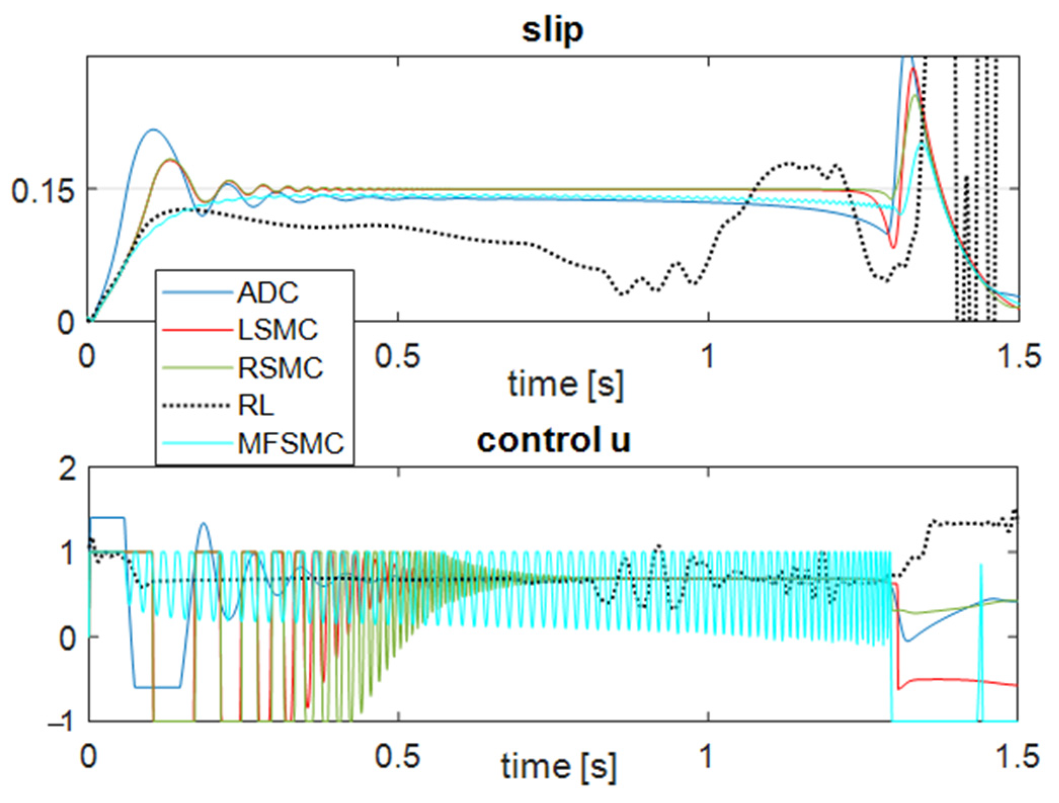
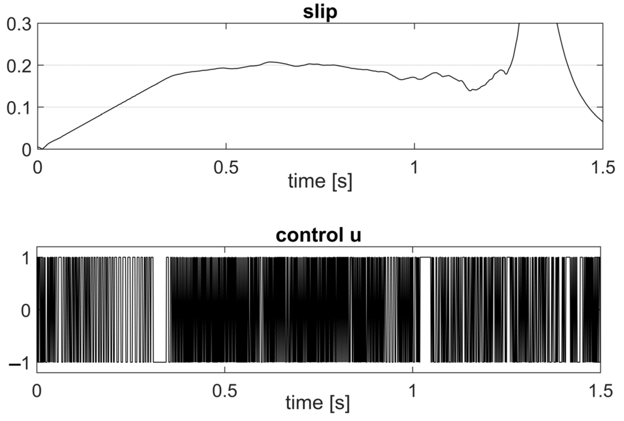
The performance index is next measured for all compared controllers, to assess their performance. The set-point tracking results obtained with the controllers LSMC, RSMC, ADC, RL, and MFSMC are shown below in Figure 6 and with the PSSMC in Figure 7. The performance measured with LSMC is , the one with the RSMC controllers is , that obtained with ADC is , that obtained with the RL controller is , for the MFSMC and for the PSSMC . Throughout the braking process, the index of the first sample at which the lower wheel speed drops below 10 rad/s are, respectively, NLSMC = 1272, NRSMC = 1272, NADC = 1262, NRL = 1330, NMFSMC = 1275, NPSSMC = 1298. Revealing that the LSMC and RSMC controllers lead to very similar braking scenarios in terms of the car speed and measured performance.
These scenarios are also not very far from the braking scenario with the ADC controller, in the sense that the car speed decreases to 10 rad/s in about the same time (1.262 s vs. 1.272 s with the LSMC and RSMC controllers). In any case, both the LSMC and the RSMC controllers offer superior performance compared to the rest of the ADC, RL, MFSMC and PSSMC controllers in terms of the measured performance index. Although the RL controller displays a poorer performance (of about two orders of magnitude), it is noticeable that the braking learning was performed without knowing the ABS dynamics. The MFSMC controller lies within a similar model-free paradigm, since the simplified model attached to the ABS dynamics makes little use of process knowledge in the control design pipeline. The PSSMC structure reveals a complex design with many tuning parameters and it is better than the RL controller.
From a controller complexity viewpoint, the ADC controller requires only two tuning parameters () which is mostly advantageous with respect to the RSMC controller with three tunable parameters and the LSMC with five tunable parameters. However, the performance of the LSMC and the RSMC is not sensitive but rather robust to various choices of that were introduced for numerical convenience. The remaining number of parameters, one for RSMC and two for LSMC, turn the two controllers into attractive real-time implementations.
Concerning the computational burden of the compared control algorithms, the execution times were measured on a PC having base frequency of 2 GHz and clock precision of s. The allotted controller computing time for the entire braking scenario experiment lasting for 1.5 s is , , , , , . These measured times correspond to 1500 calls of the controller calculation function with sampling period of 1 millisecond. Meaning that even in the case of the RL controller, the time required to run one call falls below 1 millisecond. The measured allotted computing times include all necessary double-precision operations for calculating the control input, including numerical evaluation of the integrals and derivatives, multiplications, and additions. With proper optimizations, these controllers can be implemented on modern hardware. From computational perspective, the RSMC and LSMC are more efficient by almost an order of magnitude in terms of measured allotted computing times. While the NN-based RL controller is not the most demanding due to the many operations involved in NN evaluation, the PSSMC appears the most time consuming due to its complexity and many operations.
In a following step, the best achievable performance of the LSMC and RSMC controllers is verified. To this end, the parameters of the LSMC and the parameter of the RSMC are searched by optimizing for the test scenario under aforementioned conditions (180 rad/s initial braking speed and 0.15 slip set point obtained by first order lag filtering). The optimization is performed using a genetic algorithm (GA). The values of the parameters are searched for in the domains for the LSMC and in the domain for the RSMC. These domains also act as lower and upper bounds for the optimization variables throughout the numerical search process. Other settings were: a number of 50 search agents, 5% out of the total number of agents is the number of individuals to survive the next generation, crossover fraction is 80%, maximum 5000 generations. The GA solver parameters were set to ensure convergence to approximately the same solution on five runs.
The best values of the performance index are for the LSMC (for ) and for the RSMC (obtained for ). On one hand, the best performance values are not very far from those obtained with the initial settings of the LSMC and RSMC parameters. Yet, the result shows that the LSMC structure has slightly better control capability over the RSMC structure. Nevertheless, the control performance reveals itself as a robust one and undoubtedly superior over the other control strategies proposed for comparisons.
5. Conclusions
The ABS control system intends to streamline the braking process, while maintaining the car’s road maneuverability. The LSMC and RSMC controllers designed with included uncertainties had a positive impact on the performance of the control system behavior. This attests that, even by model order reduction and despite the strongly nonlinear process behavior, the performance is not significantly degraded, leading to a robust control behavior.
The obtained performance may vary under different road conditions and controllers’ retuning may be required. Usually, the low-level ABS braking control system operates under a higher-level supervisory logic where the surface detection task and the switching between appropriate controllers is implemented.
Especially in the braking system control design, controller robustness is a critical necessity because the braking system is affected by a large parameter variations; the weight load on the car, the tire inflation state and wear, the road-tire contact surface and the road surface profile combined with the car speed all influence the braking process. Therefore, in the model-based control design paradigm, the goal is to achieve control performance under large parameter uncertainty.
For the proposed controllers, the performance comparisons with other similar or different control strategies reveal that the advantage of the LSMC and RSMC lies with the reduced number of tuning parameters and robust control performance under process variation and controller parameters selection. Finding robust, high-performance controllers with few tunable parameters is not trivial in practice, however, the LSMC and RSMC may be preferable over more complex implementations. This observation offers a significant incentive to validate the proposed approach on commercial braking systems, as a future goal.
Author Contributions
All authors have contributed equally to this work. All authors have read and agreed to the published version of the manuscript.
Funding
This work was supported by a grant from the Romanian Ministry of Education and Research, CNCS-UEFISCDI, project number PN-III-P1-1.1-TE-2019-1089, within PNCDI III.
Conflicts of Interest
The authors declare no conflict of interest.
Appendix A
For deriving the LSMC control law (8), consider the first case 1.(a) corresponding to for which . Note in the first place that . By the triangle inequality, it is checked that holds. Since , then in order to ensure that for , it suffices to select a control that fulfils . A firm selection is with , which is equivalent to
The case 1.(b) corresponds to for which . Since , the control which ensures that for and also fulfils is , which is equivalent to
The case 2.(a) refers to for which . It is similar with the case 1.(b) therefore, one control input which fulfils is found as in (A2).
Finally, the case 2.(b) is valid whenever for which . Being similar to the case 1.(a), one control input fulfilling the condition is expressible as in (A1).
The control input in all the four subcases will be correctly captured and compactly written by the general form (A1), depending on the sign of the product .
References
- Formentin, S.; Novara, C.; Savaresi, S.M.; Milanese, M. Active braking control system design: The D2-IBC Approach. IEEE Trans. Mech. 2015, 20, 1573–1584. [Google Scholar] [CrossRef]
- Liu, Y.; Sun, J. Target slip tracking using gain-scheduling for antilock braking system. In Proceedings of the IEEE American Control Conference, Seattle, WA, USA, 21–23 June 1995; pp. 1178–1182. [Google Scholar]
- Unsal, C.; Kachroo, P. Sliding mode measurement feedback control for antilock braking systems. IEEE Trans. Control Syst. Technol. 1999, 7, 271–281. [Google Scholar] [CrossRef] [Green Version]
- Tang, Y.; Zhan, X.; Zhang, D.; Zhao, G.; Guan, X. Fractional order sliding mode controller design for antilock braking systems. Neurocomputing 2013, 111, 122–130. [Google Scholar] [CrossRef]
- Mirzaeinejad, H.; Mirzaei, M. A novel method for non-linear control of wheel slip in anti-lock braking systems. Control Eng. Pract. 2010, 18, 918–926. [Google Scholar] [CrossRef]
- Chereji, E. Soluții de Reglare în Mod Alunecător Pentru un Echipament de Laborator cu Frânare cu ABS. Bachelor’s Thesis, Politehnica University of Timisoara, Timisoara, Romania, June 2019. [Google Scholar]
- Safe Braking. 50 Years Start of Developing Bosch’s Anti-Lock Braking System ABS. Available online: https://www.bosch.com/stories/beginnings-of-abs/ (accessed on 19 August 2020).
- Mercedes-Benz and the Invention of the Anti-Lock Braking System: ABS, Ready for Production in 1978. Available online: https://media.daimler.com/marsMediaSite/en/instance/ko/Mercedes-Benz-and-the-invention-of-the-anti-lock-braking-system-ABS-ready-for-production-in-1978.xhtml?oid=9913502 (accessed on 19 August 2020).
- Robert Bosch GmbH. Bosch Automotive Handbook, 8th ed.; Bentley Publishers: Cambridge, MA, USA, 2011. [Google Scholar]
- Lua, C.A.; Toledo, B.C.; di Gennaro, S.; Martinez-Gardea, M. Dynamic control applied to a laboratory antilock braking system. Math. Probl. Eng. 2015. [Google Scholar] [CrossRef]
- Drakunov, S.; Ozguner, U.; Dix, P.; Ashrafi, B. ABS control using optimum search via sliding modes. IEEE Trans. Control Syst. Technol. 1995, 3, 79–85. [Google Scholar] [CrossRef] [Green Version]
- Will, A.B.; Hui, S.; Zak, S.H. Sliding mode wheel slip controller for an antilock braking system. Int. J. Veh. Des. 1998, 19, 523–539. [Google Scholar]
- Ivanov, V.; Savitski, D.; Shyrokau, B. A survey of traction control and antilock braking systems of full electric vehicles with individually controlled electric motors. IEEE Trans. Veh. Technol. 2015, 64, 3878–3896. [Google Scholar] [CrossRef]
- Pretagostini, F.; Ferranti, L.; Berardo, G.; Ivanov, V.; Shyrokau, B. Survey on wheel slip control design strategies, evaluation and application to antilock braking systems. IEEE Access 2020, 8, 10951–10970. [Google Scholar] [CrossRef]
- The Laboratory Anti-Lock Braking System Controlled from PC—User Manual; Inteco Sp.: Krakow, Poland, 2007.
- Radac, M.B.; Precup, R.E.; Preitl, S.; Tar, J.K.; Burnham, K.J. Tire slip fuzzy control of a laboratory anti-lock braking system. In Proceedings of the European Control Conference, Budapest, Hungary, 23–26 August 2009; pp. 940–945. [Google Scholar]
- Harifi, A.; Aghagolzadeh, A.; Alizadeh, G.; Sadeghi, M. Designing a sliding mode controller for slip control of antilock brake systems. Transp. Res. Part C Emerg. Technol. 2008, 16, 731–741. [Google Scholar] [CrossRef]
- Lin, C.M.; Hsu, C.F. Self-learning fuzzy sliding-mode control for antilock braking systems. IEEE Trans. Control Technol. 2003, 11, 273–278. [Google Scholar] [CrossRef] [Green Version]
- Bartoszewicz, A.; Adamiak, K. Discrete-time sliding-mode control with a desired switching variable generator. IEEE Trans. Autom. Control 2019, 65, 1807–1814. [Google Scholar] [CrossRef]
- Bartoszewicz, A.; Adamiak, K. Model reference discrete-time variable structure control. Int. J. Adapt. Control Signal Process. 2019, 32, 1440–1452. [Google Scholar] [CrossRef]
- Shah, D.; Mehta, A.; Patel, K.; Bartoszewicz, A. Event-triggered discrete higher-order SMC for networked control system having network irregularities. IEEE Trans. Ind. Inf. 2020, 16, 6837–6847. [Google Scholar] [CrossRef]
- Latosinski, P.; Bartoszewicz, A. Model reference DSMC with a relative degree two switching variable. IEEE Trans. Autom. Control 2020. [Google Scholar] [CrossRef]
- Schinkel, M.; Junt, K. Anti-lock braking control using a sliding mode like approach. In Proceedings of the American Control Conference, Anchorage, AK, USA, 8–10 May 2002; pp. 2386–2391. [Google Scholar]
- Lin, C.M.; Hsu, C.F. Neural-network hybrid control for antilock braking systems. IEEE Trans. Neural Netw. 2003, 14, 351–359. [Google Scholar] [CrossRef]
- Wu, M.C.; Shih, M.C. Simulated and experimental study of hydraulic anti-lock braking system using sliding-mode PWM control. Mechatronics 2003, 13, 331–351. [Google Scholar] [CrossRef]
- Peric, S.L.; Antic, D.S.; Milovanovic, M.B.; Mitic, D.B.; Milojkovic, M.T.; Nikolic, S.S. Quasi-sliding mode control with orthogonal endocrine neural network-based estimator applied in anti-lock braking system. IEEE Trans. Mech. 2016, 21, 754–764. [Google Scholar] [CrossRef]
- Topalov, A.V.; Oniz, Y.; Kayacan, E.; Kaynak, O. Neuro-fuzzy control of antilock braking system using sliding mode incremental learning algorithm. Neurocomputing 2011, 74, 1883–1893. [Google Scholar] [CrossRef]
- Kayacan, E.; Oniz, Y.; Kaynak, O. A grey system modeling approach for sliding-mode control of antilock braking system. IEEE Trans. Ind. Electron. 2009, 56, 3244–3252. [Google Scholar] [CrossRef]
- Gong, X.; Qian, L.; Ge, W.; Wang, L. Research on the anti-disturbance control method of brake-by-wire unit for electric vehicles. World Electr. Veh. J. 2019, 10, 44. [Google Scholar] [CrossRef] [Green Version]
- Sardarmehni, T.; Heydari, A. Sub-optimal switching in anti-lock brake systems using approximate dynamic programming. IET Control Theory Appl. 2019, 13, 1413–1424. [Google Scholar] [CrossRef]
- He, Y.; Lu, C.; Shen, J.; Yuan, C. Design and analysis of output feedback constraint control for antilock braking system with time-varying slip ratio. Math. Probl. Eng. 2019. [Google Scholar] [CrossRef]
- Lin, C.L.; Hung, H.C.; Li, J.C. Active control of regenerative brake for electric vehicles. Actuators 2018, 7, 84. [Google Scholar] [CrossRef] [Green Version]
- Radac, M.B.; Precup, R.E. Data-driven model-free slip control of anti-lock braking systems using reinforcement Q-learning. Neurocomputing 2018, 275, 317–329. [Google Scholar] [CrossRef]
- Bhat, S.P.; Bernstein, D.S. Finite-time stability of continuous autonomous systems. SIAM J. Control. Optim. 2000, 38, 751–766. [Google Scholar] [CrossRef]
- Nersesov, S.G.; Ashrafiuon, H.; Ghorbanian, P. On the stability of sliding mode control for a class of underactuated nonlinear systems. In Proceedings of the 2010 American Control Conference, Baltimore, MD, USA, 30 June–2 July 2010; pp. 3446–3451. [Google Scholar]
- Lua, C.A.; di Gennaro, S.; Morales, M.E.S. Nonlinear adaptive controller applied to an antilock braking system with parameters variations. Int. J. Control Autom. Syst. 2017, 15, 2043–2052. [Google Scholar]
- Precup, R.E.; Radac, M.B.; Roman, R.C.; Petriu, E.M. Model-free sliding mode control of nonlinear systems: Algorithms and experiments. Inf. Sci. 2017, 381, 176–192. [Google Scholar] [CrossRef]
- Oliveira, T.R.; Hsu, L.; Peixoto, A.J. Output-feedback global tracking for unknown control direction plants with application to extremum-seeking control. Automatica 2011, 47, 2029–2038. [Google Scholar] [CrossRef]
Figure 1.
The anti-lock braking system (ABS) model diagram.

Figure 2.
The characteristics .

Figure 3.
The dependence for the reaching-law-based sliding mode controller (RSMC) stability analysis case.
Figure 3.
The dependence for the reaching-law-based sliding mode controller (RSMC) stability analysis case.
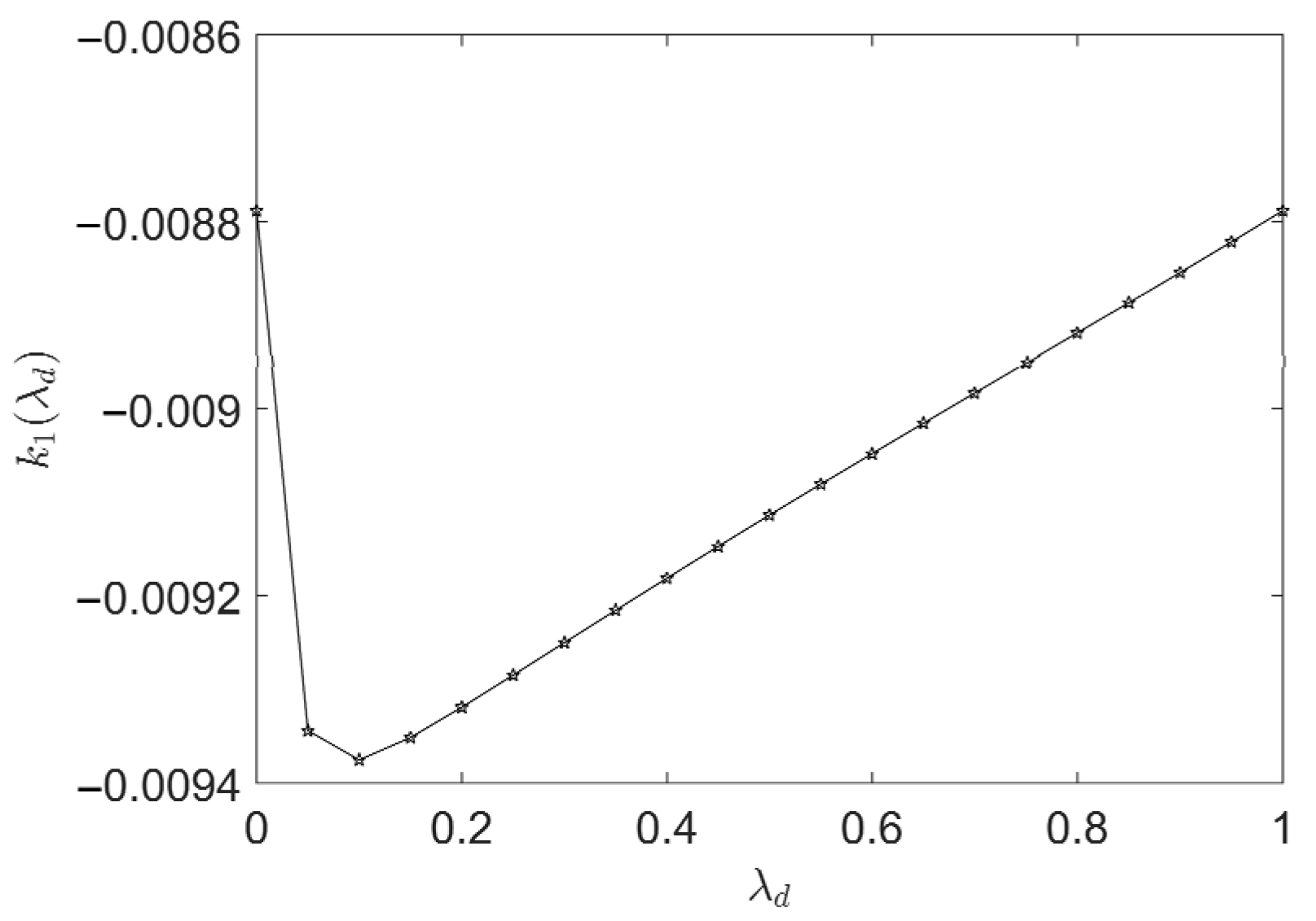
Figure 4.
The family of first order differential equations for the RSMC stability analysis case.

Figure 5.
The slip feedback control system where the slip controller is replaceable with any of the following designed controllers.
Figure 5.
The slip feedback control system where the slip controller is replaceable with any of the following designed controllers.

Figure 6.
The slip control results obtained with the Lyapunov-based sliding mode controller (LSMC), RSMC, active dynamic controller (ADC), reinforcement learning (RL) and model-free sliding-mode controller (MFSMC) structures.
Figure 6.
The slip control results obtained with the Lyapunov-based sliding mode controller (LSMC), RSMC, active dynamic controller (ADC), reinforcement learning (RL) and model-free sliding-mode controller (MFSMC) structures.

Figure 7.
The slip control result obtained with the periodic switching sliding mode controller (PSSMC) structure.
Figure 7.
The slip control result obtained with the periodic switching sliding mode controller (PSSMC) structure.

Publisher’s Note: MDPI stays neutral with regard to jurisdictional claims in published maps and institutional affiliations. |
© 2020 by the authors. Licensee MDPI, Basel, Switzerland. This article is an open access article distributed under the terms and conditions of the Creative Commons Attribution (CC BY) license (http://creativecommons.org/licenses/by/4.0/).
Share and Cite
MDPI and ACS Style
Chereji, E.; Radac, M.-B.; Szedlak-Stinean, A.-I. Sliding Mode Control Algorithms for Anti-Lock Braking Systems with Performance Comparisons. Algorithms 2021, 14, 2. https://0-doi-org.brum.beds.ac.uk/10.3390/a14010002
AMA Style
Chereji E, Radac M-B, Szedlak-Stinean A-I. Sliding Mode Control Algorithms for Anti-Lock Braking Systems with Performance Comparisons. Algorithms. 2021; 14(1):2. https://0-doi-org.brum.beds.ac.uk/10.3390/a14010002
Chicago/Turabian StyleChereji, Emanuel, Mircea-Bogdan Radac, and Alexandra-Iulia Szedlak-Stinean. 2021. "Sliding Mode Control Algorithms for Anti-Lock Braking Systems with Performance Comparisons" Algorithms 14, no. 1: 2. https://0-doi-org.brum.beds.ac.uk/10.3390/a14010002
Note that from the first issue of 2016, this journal uses article numbers instead of page numbers. See further details here.