Hardness of an Asymmetric 2-Player Stackelberg Network Pricing Game †


1
Dipartimento di Scienze Umanistiche e Sociali, Università di Sassari, 21, 07100 Sassari SS, Italy
2
Dipartimento di Ingegneria dell’Impresa, Università di Roma “Tor Vergata”, 50, 00133 Roma (RM), Italy
3
Dipartimento di Ingegneria e Scienze dell’Informazione e Matematica, Università degli Studi dell’Aquila, 67100 L’Aquila AQ, Italy
4
Istituto di Analisi dei Sistemi ed Informatica, CNR, Via dei Taurini, 19 - 00185 Roma (RM), Italy
*
Author to whom correspondence should be addressed.
†
This work was partially supported by the “Fondo di Ateneo per la Ricerca 2019” grant of the University of Sassari and by the project E89C20000620005 “ALgorithmic aspects of BLOckchain TECHnology” (ALBLOTECH).
Algorithms 2021, 14(1), 8; https://0-doi-org.brum.beds.ac.uk/10.3390/a14010008
Submission received: 27 November 2020
/
Revised: 23 December 2020
/
Accepted: 24 December 2020
/
Published: 31 December 2020
(This article belongs to the Special Issue Graph Algorithms and Network Dynamics)
Abstract
:Consider a communication network represented by a directed graph of n nodes and m edges. Assume that edges in E are partitioned into two sets: a set C of edges with a fixed non-negative real cost, and a set P of edges whose costs are instead priced by a leader. This is done with the final intent of maximizing a revenue that will be returned for their use by a follower, whose goal in turn is to select for his communication purposes a subnetwork of Gminimizing a given objective function of the edge costs. In this paper, we study the natural setting in which the follower computes a single-source shortest paths tree of G, and then returns to the leader a payment equal to the sum of the selected priceable edges. Thus, the problem can be modeled as a one-round two-player Stackelberg Network Pricing Game, but with the novelty that the objective functions of the two players are asymmetric, in that the revenue returned to the leader for any of her selected edges is not equal to the cost of such an edge in the follower’s solution. As is shown, for any and unless , the leader’s problem of finding an optimal pricing is not approximable within , while, if G is unweighted and the leader can only decide which of her edges enter in the solution, then the problem is not approximable within . On the positive side, we devise a strongly polynomial-time -approximation algorithm, which favorably compares against the classic approach based on a single-price algorithm. Finally, motivated by practical applications, we consider the special cases in which edges in C are unweighted and happen to form two popular network topologies, namely stars and chains, and we provide a comprehensive characterization of their computational tractability.
1. Introduction
Leader–follower games were introduced by von Stackelberg in 1934 [1], with the aim of modeling heterogeneous markets, namely markets in which one or more players are in a leadership position, and can in practice manipulate the market to their own advantage, by directly influencing the choices of the remaining subjects. In the basic formulation, the game is played by only two players: the leader who moves first and the follower who observes the leader’s move and then makes his (throughout the paper, we adopt the convention of referring to the leader and the follower with female and male pronouns, respectively) own move, after which the game is over. The strategic aspect of the game consists of the fact that the follower computes a solution by optimizing an objective (public) function, while the leader has her own objective function, which is, by the way, computed over the solution selected by the follower. In this way, to optimize her revenue, the leader has to entail in her move the optimal response which will be given by the follower.
Leader–follower games have received considerable attention from the computer science community, mainly because the Internet is a perfect paradigm of heterogenous market. In fact, the Internet is a vast, pervasive electronic market mainly composed of millions of independent end-users, whose actions are by the way influenced by the owners of physical/logical portions of the network, for instance service providers. Under this perspective, it turns out to be particularly intriguing the problem of analyzing the antagonism emerging between leaders and followers whenever a communication subnetwork must be allocated.
1.1. Stackelberg Network Pricing Games
Network games can be easily regarded as Stackelberg games, as soon as a situation arises in which a subset of dominant players controls a higher-level decision phase in which part of the game instance is set, for example by routing a substantial amount of a network flow [2] or by deciding the cost of a subset of network arcs. In particular, games of this latter type, which are of interest for this paper, are widely known as Stackelberg Network Pricing Games (SNPGs).
A SNPG can be formalized as follows: We are given either a directed or an undirected graph , with an edge cost function , while edges in P need to be priced by the leader. In the following, we assume that and . As usual, we also permit the existence of parallel pairs of weighted and priceable edges. Then, the leader moves first and chooses a pricing function for her edges, in an attempt to maximize her objective function , where denotes the decision which will be taken by the follower, consisting in the choice of a subgraph of G. This notation stresses the fact that the leader’s problem is implicit in the follower’s decision. Once observed the leader’s choice, the follower reacts by selecting a subgraph of G which minimizes his objective function , parameterized in p. Note that the leader’s strategy affects both the follower’s objective function and the set of feasible decisions, while the follower’s choice only affects the leader’s objective function. Throughout the paper, we naturally assume that is price-additive, i.e., . This means the leader decides edge prices having in mind that her revenue equals the overall price of her selected edges.
The most immediate SNPG is that in which we are given two specified nodes in G, say , and the follower wants to travel along a shortest path in G between s and t (see [3] for a survey). This problem has been shown to be APX-hard [4], as well as not approximable within a factor of unless P = NP [5], while an -approximation is provided in [6]. For the case of multiple followers (each with a specific source-destination pair), Labbé et al. [7] derived a bilevel LP formulation of the problem (and proved NP-hardness), while Grigoriev et al. [8] presented algorithms for a restricted shortest path problem on parallel edges. Another basic SNPG is that in which the follower wants to use a minimum spanning tree of G (now considered as undirected). For this game, in [9], the authors proved the APX-hardness already when the number of possible edge costs is 2 and gave an -approximation algorithm. Better approximations are possible when the leader can also choose the positions of her edges [10].
All the above examples fall within the class of SNPGs handled by the general model proposed in [11], which encompasses all the cases where each follower aims at optimizing a polynomial-time network optimization problem in which the cost of the network is given by the sum of prices and costs of contained edges, namely
Thus, in this model, we have that coincides with once this is restricted to the leader’s edges. To this respect, the leader’s and follower’s maximization and minimization functions are therefore symmetric. The authors showed that all SNPGs in this class can be tightly approximated within , for any , where k denotes the number of followers, while is the i-th harmonic number.
1.2. Asymmetric SNPGs
In this paper, we focus on a natural asymmetric SNPG, namely that in which the follower aims at building a single-source shortest paths tree (SPT) of G rooted at a given node r. More formally, our game, which we call Asymmetric Stackelberg Shortest Paths Tree (ASSPT), can be described as the following bilevel optimization problem (all the paths are assumed to be directed):
- Instance: A directed graph , a function , and a source node .
- Leader feasible solution: A pricing .
- –
- Follower feasible solution: A spanning arborescence of G rooted at r (after edges in P have been priced).
- –
- Follower objective: Find a feasible solution minimizing the sum of all the path costs in T from r to any node in G, namely, denoting by the number of paths in T emanating from r and using e, minimize
- Leader objective: Find a feasible pricing maximizing the revenue w.r.t. an optimal solution, say , selected by the follower, namely minimize
This game is clearly asymmetric, since does not coincide with once this is restricted to priced edges, and finds its motivation in SPT-based routing on the Internet. Here, an Autonomous System (i.e., the leader) controlling part of the underlying network infrastructure could suitably adjust the costs of her edges in order to influence the choice of a follower in selecting a subnetwork satisfying his specific connectivity requirements. Actually, if the follower needs to provide a broadcasting service from a source to a set of destination nodes (i.e., final users which will in their turn pay for the service a cost proportional to the sum of the edge costs along a corresponding path from the source node), then buying an SPT rooted at the source allows the follower to certify the usage of a cheapest routing path.
With the study of the ASSPT game, we continue in the effort of analyzing the computational aspects of SPT pricing games, which started in [19,20] with the symmetric version of the game (i.e., that in which the leader’s revenue for each selected edge is given by its price multiplied by the number of paths—emanating from the source—it belongs to). For this game, Bilo et al. [19] proved that finding an optimal pricing for the leader’s edges is NP-hard, as soon as , while it is polynomial-time solvable when is constant. A faster algorithm for the latter case was improved by Cabello [20]. In the following, as usual, we assume that, when multiple optimal solutions are available for the follower, he selects an optimal solution maximizing the leader’s revenue (At a first glance, this rule looks in contrast with the antagonistic nature of the game. However, if this rule is relaxed, then it is easy to see that an optimal solution for the leader can only be reached within any arbitrary small subtractive term.).
1.3. Our Results
Throughout the paper, we analyze the ASSPT game under several respects. More precisely, we first study the complexity of the game, and we show that finding an optimal pricing for the leader’s edges is an extremely difficult task, even under strongly restrictive assumptions. Indeed, we show that for every , the ASSPT game is not approximable within a factor of , unless P = NP. Then, we turn our attention to the unweighted ASSPT game, i.e., the one in which for any , while , and we prove that, for every , the game is not approximable within a factor of , unless .
Then, we turn our attention to the development of an approximation algorithm for the ASSPT game, and we devise a pricing strategy that in time returns an -approximation of the optimal leader’s revenue. Although our algorithm leaves an gap open with the corresponding inapproximability result, remarkably, its running time is strongly polynomial (i.e., it does not depend on the magnitude of the costs of the edges in C). Therefore, it compares favorably with the powerful but non-strongly polynomial single-price algorithm [11], which has a provably logarithmic approximation ratio for any symmetric SNPGs in which is of the form (1), while in contrast we show that for the ASSPT game it can only guarantee an factor.
Finally, motivated by practical applications, we study the ASSPT game when edges in C are unweighted and happen to form two popular network communication topologies, namely stars and chains. As far as the star topology is concerned, we first show an equivalence of the ASSPT game with the well-studied Rooted Maximum Leaf Outbranching (RMLO) problem, which asks for finding a spanning arborescence rooted at some prescribed vertex of a digraph with the maximum number of leaves. This problem is known to be NP-hard already on directed acyclic graphs (DAGs), as well as 92-approximable [21,22]. Thus, these results immediately extend to the ASSPT game on unweighted stars. Moreover, we show the APX-hardness of such a game even if G is actually a DAG, and this inapproximability carries over to the RMLO problem on DAGs, as is shown below, which is a result of independent interest. Concerning the chain topology, we show that, if G is a DAG, then our approximation algorithm returns an optimal pricing, even in the weighted case. On the other hand, if G is not a DAG, then we prove the ASSPT game becomes NP-hard, and so the problem of finding a constant-ratio approximation algorithm, for which we conjecture the existence, remains a challenging open problem.
The rest of the paper is organized as follows. Section 2 contains inapproximability results. Section 3 presents our approximation algorithm, along with a bad instance example for the single-price algorithm. Section 4 deals with the star and the chain topology. Section 5 concludes the paper and suggests possible future work.
2. Non-Approximability Results
In this section, we prove that the ASSPT game along with some basic variants of it are very hard to approximate. For the sake of simplifying the presentation, we first analyze a binary pricing version of the game, denoted as , in which the leader is constrained to price her edges either or . Then, we start by proving the following:
Theorem 1.
For every , with , and for every constant , the game is not approximable within a factor of , unless , even on DAGs.
Proof.
The reduction is from the Maximum Independent Set (MIS) problem, i.e., the problem of finding a maximum cardinality set I of vertices of a given undirected graph G of n vertices such that no pair of vertices in I is linked by an edge of G. More precisely, we describe how a graph G of n vertices—which is provided as an instance of the MIS problem—can be transformed into an instance of the on a graph of vertices. The claim then follows from the fact that the MIS problem is not approximable within a factor of for every constant , unless , even if G is a connected graph [23].
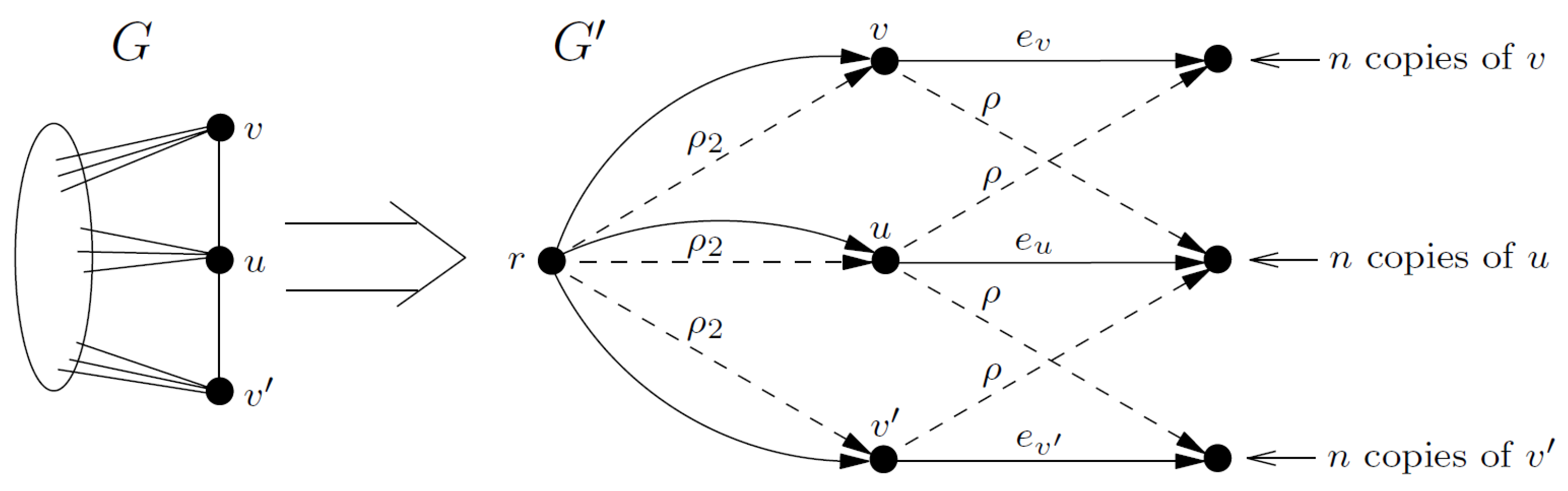
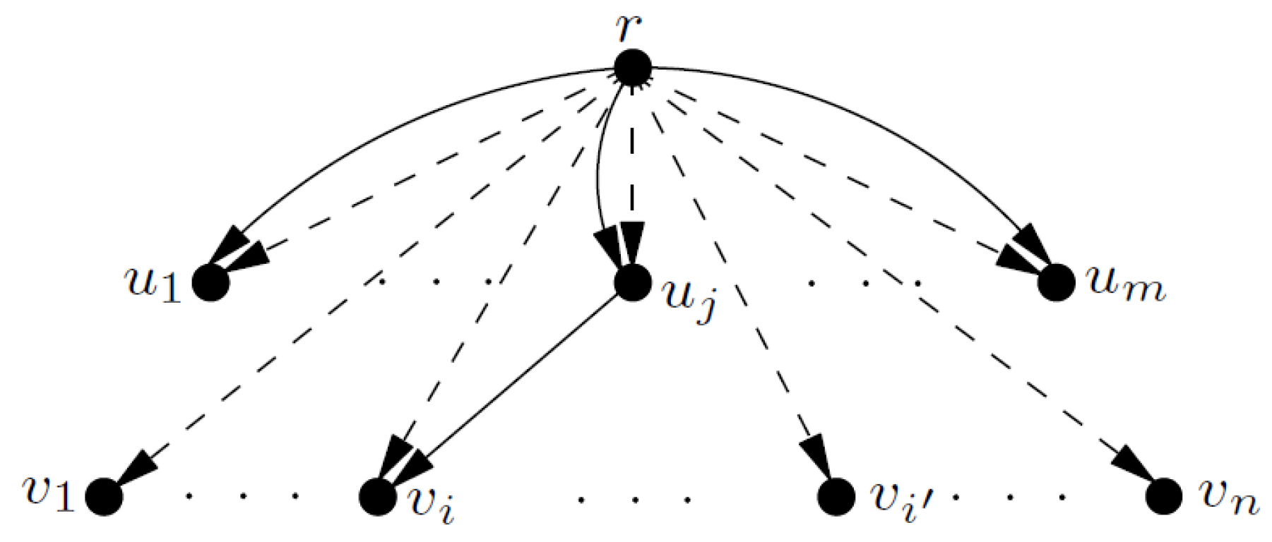
The reduction works as follows. From a given undirected connected graph of n vertices, we build a three-layered DAG . The first layer of contains the root vertex r (w.l.o.g., we can assume that ), the second layer of contains a copy of all the vertices of G, while the third layer of contains n copies of all the vertices of G. We observe that has vertices. The set of fixed-cost edges is the following: there is an edge of cost from r to every vertex in the second layer, and there is an edge of cost from a vertex u in the second layer to all the copies of vertex v in the third layer iff . The set P of leader’s edges is the following: there is an edge from r to every vertex in the second layer, and every vertex u in the second layer has an outgoing edge towards each of its copies in the third layer. An example of the reduction is shown in Figure 1.
By the connectivity property of G, there is a fixed-cost path of length from r to every vertex in the second layer, and a fixed-cost path of length from r to every vertex in the third layer. Let be equal to if , and otherwise. In what follows, we prove that every pricing defines an independent set of G, and yields a revenue of at most . Moreover, we also prove that for every independent set I of G, there exists a pricing p yielding a revenue of at least , and such that . The claim then follows from the non-approximability result of the MIS problem and because has vertices. Indeed, for the sake of contradiction, assume that is approximable within a factor of , for some constant , by a polynomial-time algorithm . Let be an optimal pricing such that is a maximum independent set of G and let p be the pricing computed by . The revenue yielded by is of at least , while the revenue yielded by p is of at most . Since , we have that , and, therefore, can be used to compute—in polynomial time—an -approximate solution for the MIS problem instance. However, this contradicts the fact that the MIS problem is not approximable within a factor of , for any constant , unless .
Let denote any leader’s edge from a vertex u in the second layer to one of its copies in the third layer. For a pricing p, let denote the set of vertices u having some with being part of an SPT of . The edge is contained in an SPT of iff
From the above inequalities, we have that is contained in an SPT of and iff
This implies that, if edge is in some SPT of and , then no SPT of contains the edge , for every vertex v such that . As a consequence, the set always defines an independent set of G. Moreover, observe that the revenue yielded by p is at most for the leader’s edges outgoing from r, and at most for the other edges. Therefore, the total revenue yielded by p is at most .
To complete the proof, let I be an independent set of G. The pricing p that satisfies the equalities in (2) for every and for every , yields a revenue of at least , and defines an independent set such that . □
From the above theorem, we can easily derive the following general result:
Theorem 2.
For every , the ASSPT game is not approximable within a factor of , unless , even on DAGs where fixed-cost edges have all cost 1.
Proof.
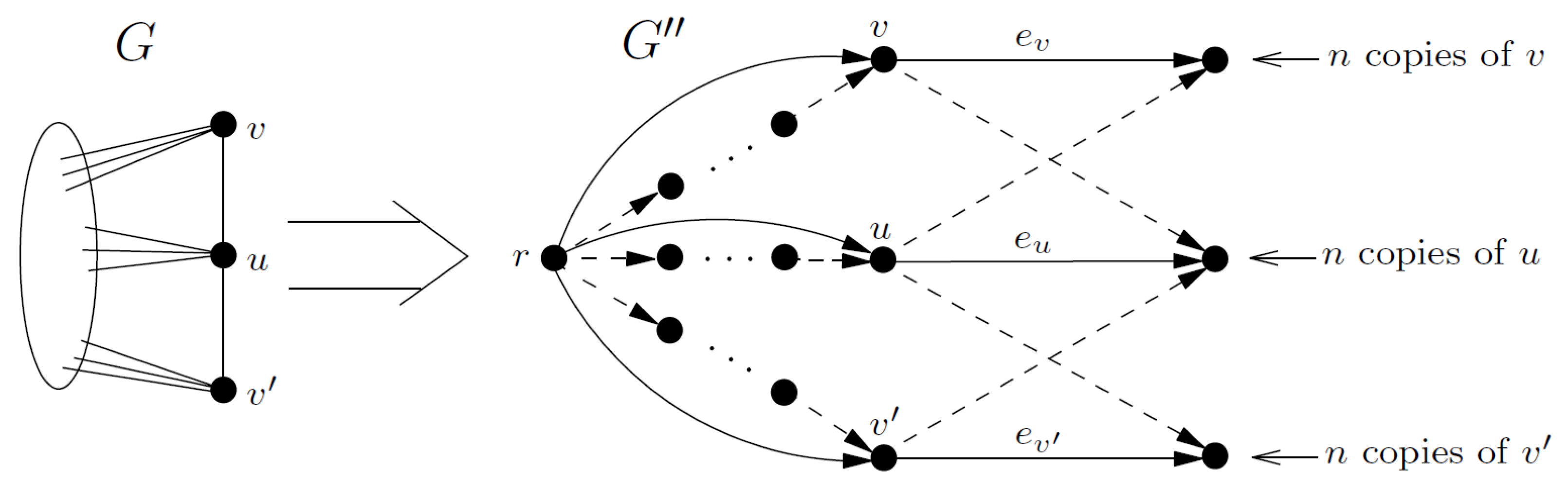
Consider the DAG built in the reduction of Theorem 1 for the case and , which implies . Build a graph from a copy of by replacing every fixed-cost edge of cost k with k edges all having cost 1. Figure 2 shows an example of the reduction. Observe that still contains vertices.
For a feasible pricing p, let denote the set of vertices u having some with being part of an SPT of . The edge is contained in an SPT of iff
This implies that if edge is in some SPT of and , then no SPT of contains the edge , for every vertex v such that . Therefore, is an independent set of G. Moreover, p yields a revenue of at most . In Theorem 1, we show a pricing p in yielding a revenue R of at least , where I is a maximum independent set of G. It is easy to see that pricing with p yields a revenue of at least R. This completes the proof. □
We now turn our attention to the unweighted ASSPT game, i.e., the one in which for any , while the leader’s price function is restricted to . Even in this simplified binary version, the game is very hard:
Theorem 3.
For every , the unweighted ASSPT game is not approximable within a factor of , unless , even on DAGs.
Proof.
Consider the DAG defined in the proof of Theorem 2. has been built from the DAG defined in Theorem 1 for the case and , which implies .
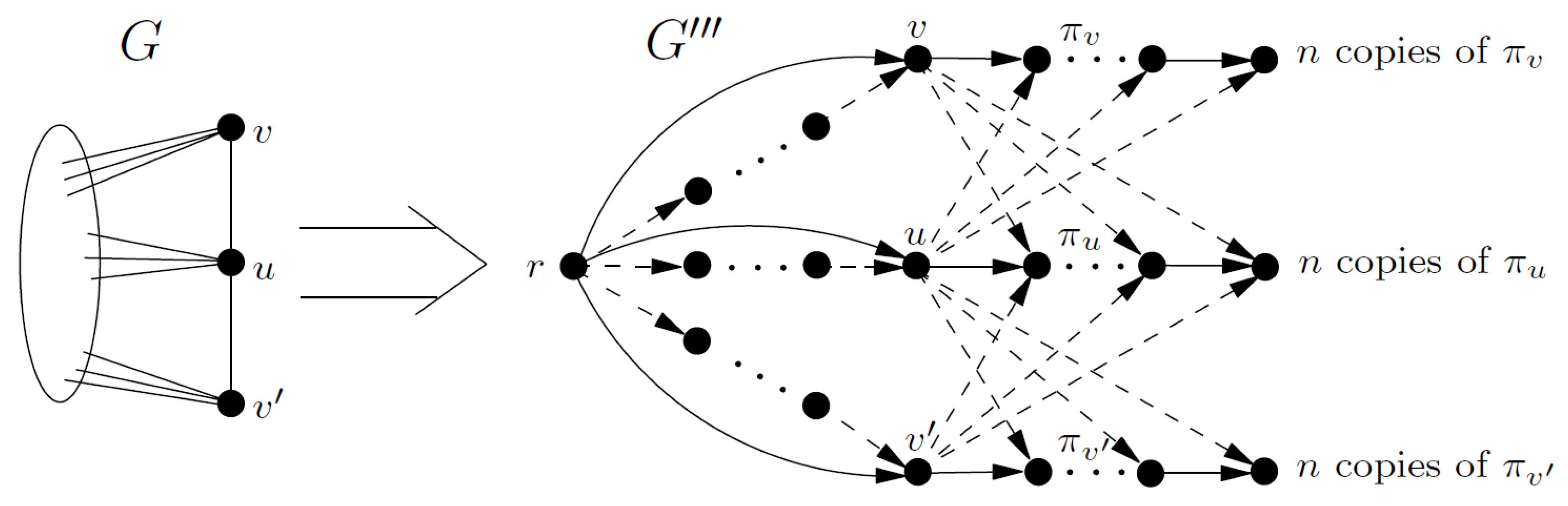
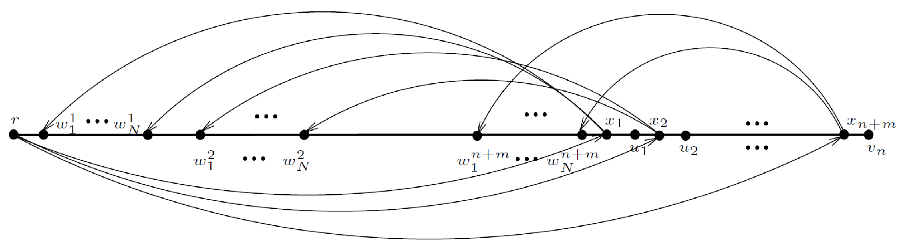
From , we build the DAG , which is obtained by replacing each edge by a path of n leader’s edges. Moreover, for every vertex and for every vertex v such that is a unit-cost edge of , we add the unit-cost edge to . As a consequence, there is a fixed-cost path of length from r to every . Figure 3 shows an example of the reduction. Observe that has vertices.
Let p be a pricing in that prices edges either 1 or . Let be a pricing in defined as follows. For an edge e incident to the root vertex, if . An edge has a price of i if the first edges of the corresponding path in are contained in an SPT of , and no SPT of contains the first edges of the corresponding path in . All the remaining edges are priced with an arbitrarily large value (observe that pricing an edge with is equivalent to pricing it with an arbitrarily large value). Observe that, if p yields a revenue of R, then so does . Indeed, an edge is contained in an SPT of iff it is contained in an SPT of . Furthermore, an edge with price i is contained in an SPT of iff the first i edges of the corresponding path are contained in an SPT of .
In the proof of Theorem 2, we show that defines an independent set of G and yields a revenue of at most . As a consequence, p defines an independent set of G and yields a revenue R of at most . Let I be a maximum independent set of G. Let p be a pricing in which prices an edge e with 1 iff , or and . Observe that p yields a revenue of . This completes the proof. □
3. A Strongly Polynomial -Approximation Algorithm
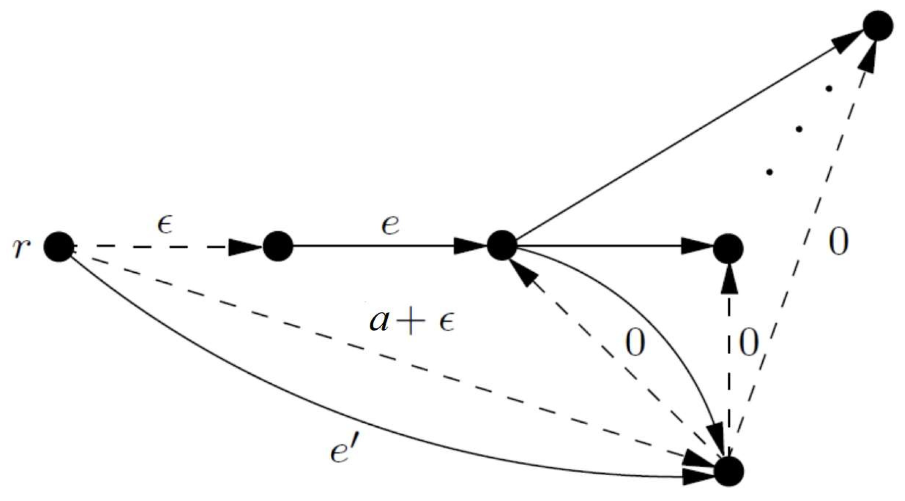
For symmetric SNPGs, Briest et al. [11] proved the existence of an algorithm, called the single-price algorithm, that guarantees an approximation of , where k denotes the number of followers. Notice that this result implies an -approximation for the symmetric version of the Stackelberg SPT game studied in [19]. Therefore, a simple question is whether the single-price algorithm provides a good approximation also for the ASSPT game. Not surprisingly, this is not the case, as illustrated in Figure 4, where we give an instance for which the single-price algorithm returns an -approximate solution. Thus, the power of the single-price algorithm seems to rely on the alignment of the leader’s and follower’s objective functions.
Besides being only -approximating, the single-price algorithm has also another drawback, namely it is not strongly polynomial, since it is polynomial in the input size, but its running time depends on the given edge costs. Indeed, for our problem, it requires the testing of different weights for the priceable edges, where is the cost of a cheapest feasible solution not containing leader’s edges. Therefore, in an effort to improve on that, we develop the following simple strategy the leader can play in order to get in strongly polynomial-time an -approximation of the maximum achievable revenue. Actually, the goal of closing the gap left open w.r.t. the corresponding inapproximability result remains a challenging open problem.
Theorem 4.
For the ASSPT problem, the pricing function p that prices each edge with is computable in time and yields a revenue of at least , where denotes distances computed in and denotes the revenue yielded by an optimal pricing.
Proof.
Let be a pricing such that . For a path , we denote by the value . Let be a path in outgoing from r such that , for every other path of outgoing from r. Clearly, . In what follows, we show that .
Let denote the edges of in the order in which they appear if we traverse starting from r. Let , for every . Moreover, for every , let us denote by the length of the (fixed-cost) subpath of going from to , where . We have that
Summing over all is, adding up the two equalities and , and rearranging the terms, we obtain
Since is a shortest path in G w.r.t. , we have that from which we get
Furthermore, notice that for every vertex v. Next, observe that every edge e with is contained in a SPT of G w.r.t. p. As a consequence, there is a SPT of G w.r.t. p that contains all the edges ’s for which . Therefore,
We conclude by observing that the upper-bound of the approximation ratio is asymptotically tight. Indeed, the digraph in Figure 4 without edge , shows an example where pricing all edges according to the formula given in the above theorem does not return a better than -approximate solution.
4. Dealing with Basic Network Topologies
In this section, motivated by practical applications, we consider the special cases in which edges in C are unweighted and happen to form two popular network communication topologies, namely stars and chains, and we provide a comprehensive characterization of their computational tractability.
4.1. Unweigthed Stars
In this section, we focus on instances where edges in C have cost 1 and form a star emanating from the source node r. We show that the problem of finding a pricing maximizing the revenue is equivalent to another problem known in literature as the Rooted Maximum Leaf Outbranching (RMLO) problem, which asks for finding a spanning arborescence rooted at some prescribed vertex of a digraph with the maximum number of leaves. This problem is known to be NP-hard even when restricted to DAGs [22] and even MaxSNP-hard on undirected graphs [24]. Moreover, it admits a 92-approximation algorithm [21]. Hence, the equivalence result immediately implies the existence of a constant-factor approximation algorithm for our problem, with the same approximation ratio. Moreover, we improve the inapproximability result for the RMLO problem by showing that it is APX-hard even for DAGs.
First, we observe that we can restrict ourselves to consider instances of pricing where all nodes can be reached by a path of priceable edges, since any other node would be reached through a single fixed-cost edge in any SPT computed by the follower, and thus it cannot influence the revenue. We can prove the following:
Lemma 1.
Let be an instance of the ASSPT game where edges in C have unitary cost and form a star rooted at r. Then, G admits a pricing with revenue greater than or equal to if and only if has a spanning arborescence rooted at r with at least k leaves.
Proof.
Let T be a spanning arborescence of rooted at r with at least k leaves. Then, we can define the following pricing for G: , if e enters into a leaf of T, 0 otherwise. It is easy to see that such a pricing yields a revenue of k, since T is a SPT of G.
On the other hand, let us consider a pricing p with revenue . Let T be the SPT computed by the follower after the leader prices her edges according to p, and let be an edge of T. Then, all the edges of the subtree of T rooted at v, say , must be priceable edges. Moreover, if is a fixed-cost edge, then all the edges in must have price 0. Now, let be the subtree of T obtained by removing every fixed-cost edge and the corresponding subtree . From the arguments given above, we have that . Now, we show that the number of leaves of , say ℓ, is at least R. Indeed, we have that
where the last inequality holds since is a subtree of a SPT of G, which implies that, for each node v, .
Now, notice that is an arborescence rooted at r of as well, but it may not span V. However, we can add priceable edges to in order to make it spanning. This does not decrease the number of leaves. □
Theorem 5.
The ASSPT game where the edges of C have unitary cost and form a star rooted at r isAPX-hard.
Proof.
The reduction is from Set Cover problem (SCP). An instance of SCP consists of a set of objects and a set of m subset of O. The objective is to find a minimum-size collection of subsets in whose union is O. In [25], it is shown that SCP is NP-hard.
Given an instance of SCP, we build the following instance of the ASSPT game. We have the root vertex r, a node for each , and a node for each . There is a fixed-cost edge (of cost 1) from r to each other node. Moreover, we have a priceable edge for each , and a priceable edge if and only if (see Figure 5). We have the following:
Lemma 2.
The instance of the ASSPT game has a pricing yielding a revenue of at least if and only if I admits a cover of size at most k.
Proof.
Let be a cover of size k for I. Then, define the following pricing: set for each , while all the other priceable edges are set to 1. It is easy to see that we obtain a unit of revenue for each , and a unit of revenue for each with , which provides a total revenue of .
Conversely, let p be a pricing yielding a revenue , and let S be the SPT computed by the follower according to p. We define two sets of nodes. Let X be the set containing every which has in S at least one outgoing priceable edge, and let Y be the set containing every which has in S an ingoing priceable edge. Then, since every node has a distance from r of at most 1, an upper bound for R is:
We now define a pricing as follows: for each , while all other edges are priced at 1. Hence, it is easy to see that yields a revenue of at least , since now each is at distance 1 from r (and there is a path of priceable edges with length 1), and since every has an ingoing leader’s edge with price 1.
Now, we modify in such a way that: (i) the revenue does not change; and (ii) in the corresponding SPT computed by the follower, every has an ingoing priceable edge with price 1. We repeatedly perform the following. Consider any that is not reached in by a priceable edge with price 1, and consider a node such that . We change from 1 to 0. This does not change the revenue, since we lose a unit of revenue from the edge , while we obtain an additional unit of revenue from the edge which is now selected by the follower.
Finally, we define a cover for I by selecting every corresponding to a node having distance 0 in . Since the revenue of is at least , and since in every is reached by a priceable edge with price 1, it follows that the size of the cover is at most k. This concludes the proof. □
To prove the APX-hardness, we restrict ourselves to instances of the SCP in which each subset has cardinality at most 3, and . Even in this case, the SCP is APX-hard [26]. We show that a -approximate algorithm for the ASSPT game would imply a -approximate algorithm for the SCP, for a suitable . Assume that we have a -approximate algorithm for the ASSPT, and let be the size of an optimum set cover for I. We have that the algorithm returns a pricing p with revenue . In the proof of Lemma 2, we show that p can be modified in order to yield a revenue of at least . Let k be the integer such that . Hence, from Lemma 2, we have that p induces a set cover of size k. Then, since , we have that:
This completes the proof. □
Therefore, from Lemma 1 and Theorem 5, we obtain the following interesting result, which improves over the NP-hardness on DAGs of the RMLO problem given in [22]:
Corollary 1.
The RMLO problem isAPX-hard even on DAGs.
4.2. Unweigthed Chains
In this section we focus on instances where edges in C form a chain, and we show that while on DAGs the problem can be solved optimally, already the seemingly easy instance in which G is not a DAG but edges in C are unweighted becomes NP-hard. However, for such an instance we conjecture the existence of a constant-ratio approximation algorithm, and this is a subject of further research.
Theorem 6.
The ASSPT game where the edges of C form a chain and G is a DAG can be solved in linear time.
Proof.
We compute for every u in linear time and we set the price of a priceable edge to . Since priceable edges are all forward edges w.r.t. the fixed-cost path, it is easy to see that in any pricing we have that for every priceable edge the distance from u to v is upper bounded by . This implies that the maximum revenue obtainable from is at most . As a consequence, we have that the revenue we can obtain from priceable edges entering in the same node v is at most . Now, the claim follows from the fact that in the distance between any two nodes is equal to the distance in between the same nodes, and hence for every node v which is the head of at least one priceable edge, we obtain revenue . □
Theorem 7.
The ASSPT game where the edges of C have unitary cost and form a chain isNP-hard.
Proof.
The reduction is again from SCP. Given an instance of SCP we build the following instance of the ASSPT game. We have the root vertex r, a node for each , and a node for each . Moreover, let N be an integer that we will fix later. We have additional nodes , , and nodes , .
The fixed-cost edges have all cost 1 and form a path (spanning all nodes) from r to . The sequence of the nodes encountered when we traverse the path from r to is the following: .
The set P of priceable edges is partitioned into two sets, say and . is defined as follows: we have an edge for each i, and an edge for each i and each j. is defined similarly as in the reduction of Theorem 5, i.e., it contains an edge for each and an edge if and only if (see Figure 6). We have the following:
Lemma 3.
In any optimal pricing p for the instance of the ASSPT game, we have and , for each , and each , when .
Proof.
Let p be an optimal pricing for and assume by contradiction that the lemma is false. Let i be the minimum index for which the property of the lemma does not hold. Let be the set of priceable edges entering in some , and let . The idea is to build a strictly better pricing from p. The pricing will lose some revenue from edges in and will obtain more revenue from edges in .
Let . We can assume that , otherwise p cannot be optimal since we can increase the revenue by simply increasing the price of every edge to . Moreover, from the optimality of p, it is clear that we can assume also that is in . Given a pricing and a node v, we will denote by the distance of v from r in . At the beginning, is defined as p except that and for every edge e not belonging to . Notice that, for every vertex v, . We first modify prices of the edges in . We repeatedly perform the following. If there is a node v such that , we consider the path P from r to v in . Let be the edges of along the path P in the order we encounter them when we traverse P from r to v. If , then we set for every . Otherwise, let k be the minimum index such that , we first decrease by , and then we set for each . We stop when there is no edge left to be decreased. Notice that, when this happens, we have decreased each edge in at most by a and it is easy to see that the revenue of obtained from edges in decreases by at most since all the edges belonging to a path in which was decreased by at least a will still be selected by the follower.
We then consider edges in . First of all we set to , for every . Let be the set of edges entering in some vertex with . For any pricing , we use to denote the set . Observe that , since priceable edges in are priced to infinity. We now modify in order to guarantee that . We repeatedly perform the following. Consider the first node when we traverse the fixed-cost path from r to such that . Since we have decreased the prices of edges in , we have belongs to . Then, we increase the price of by . Moreover, observe that for the same reason, we have that still belongs to the new SPT computed by the follower and, since the paths that are increasing their length are paths using the edge , then no other edge exits from the SPT. We repeatedly use this argument until for every node we have . Now, it is easy to see that must be equal to .
We are now ready to bound the revenue of . We have already observed that the revenue we may lose from edges in is upper bounded by , while we do not lose revenue from edges in . On the other hand, we can now bound the increment of the revenue we obtain from all the edges . Notice that every edge is now selected in . We consider two cases:
- Case
- Since is in and since , we have . Moreover, since the price of every edge increased by at least a, we have that which is strictly greater than when .
- Case
- When , no edge was selected in . As a consequence, we have which is strictly greater than when , since .Otherwise, when , we have that no edge with was selected in . Hence, since the price of every edge with has been increased by at least a, we have that , which is strictly greater than when .
□
In any optimal pricing for the instance of the ASSPT game, edges in must be priced according to the above lemma and thus they yield to a revenue of . Moreover, once edges in have fixed prices, the instance is very similar to the unweighted star instance of the reduction of Theorem 5. Indeed, every vertex and every vertex has distance 1 from r in the graph , and is defined as in the proof of Theorem 5. Hence, by using the same arguments given in the proof of Lemma 2, we can show that the instance of the ASSPT game has a pricing yielding a revenue of at least if and only if I admits a cover of size at most k. □
5. Conclusions
In this paper, we focus on an asymmetric SNPG, namely that in which the follower builds an SPT of a graph and pays a leader as the sum of the selected priced edges. Despite its apparent simplicity, such a game reveals itself as a very hard computational problem, much harder than all the previously studied—yet symmetric—SNPGs.
In search of an explanation for this discrepancy, we aim to investigate at a deeper level the mathematical nature of the corresponding bilevel optimization problem. Indeed, the asymmetry in itself does not fully explain such behavior, as suggested by an easy variation of the ASSPT game in which the follower returns to the leader only the revenue associated with the most expensive selected priced edge, which can be shown to be polynomial-time solvable. Moreover, we plan to analyze other intuitive asymmetric SNPGs, for instance that in which the follower looks for a minimum diameter spanning tree or the one in which he needs to compute a (either exact or approximate) minimum routing-cost spanning tree.
Author Contributions
Writing—review & editing, D.B., L.G. and G.P. All authors have read and agreed to the published version of the manuscript.
Funding
This research received no external funding.
Conflicts of Interest
The authors declare no conflict of interest.
References
- Kolev, S. Heinrich von Stackelberg, Market Structure and Equilibrium. J. Hist. Econ. Thought 2016, 38, 557–560. [Google Scholar] [CrossRef]
- Cole, R.; Dodis, Y.; Roughgarden, T. Pricing network edges for heterogeneous selfish users. In Proceedings of the 35th Annual ACM Symposium on Theory of Computing, San Diego, CA, USA, 9–11 June 2003; Larmore, L.L., Goemans, M.X., Eds.; ACM: New York, NY, USA, 2003; pp. 521–530. [Google Scholar] [CrossRef] [Green Version]
- Van Hoesel, C. An overview of Stackelberg pricing in networks. In Research Memorandum 043; Maastricht University, Maastricht Research School of Economics of Technology and Organization (METEOR): Maastricht, The Netherlands, 2006. [Google Scholar]
- Joret, G. Stackelberg network pricing is hard to approximate. Networks 2011, 57, 117–120. [Google Scholar] [CrossRef] [Green Version]
- Briest, P.; Chalermsook, P.; Khanna, S.; Laekhanukit, B.; Nanongkai, D. Improved Hardness of Approximation for Stackelberg Shortest-Path Pricing. In Internet and Network Economics; Saberi, A., Ed.; Springer: Berlin/Heidelberg, Germany, 2010; pp. 444–454. [Google Scholar]
- Roch, S.; Savard, G.; Marcotte, P. An approximation algorithm for Stackelberg network pricing. Networks 2005, 46, 57–67. [Google Scholar] [CrossRef] [Green Version]
- Labbé, M.; Marcotte, P.; Savard, G. A Bilevel Model of Taxation and Its Application to Optimal Highway Pricing. Manag. Sci. 1998, 44, 1608–1622. [Google Scholar] [CrossRef] [Green Version]
- Grigoriev, A.; van Hoesel, S.P.M.; van der Kraaij, A.F.; Uetz, M.; Bouhtou, M. Pricing Network Edges to Cross a River. In Proceedings of the Approximation and Online Algorithms, Second International Workshop, WAOA 2004, Bergen, Norway, 14–16 September 2004; Revised Selected Papers; Lecture Notes in Computer Science; Persiano, G., Solis-Oba, R., Eds.; Springer: Berlin/Heidelberg, Germany, 2004; Volume 3351, pp. 140–153. [Google Scholar] [CrossRef] [Green Version]
- Cardinal, J.; Demaine, E.D.; Fiorini, S.; Joret, G.; Newman, I.; Weimann, O. The Stackelberg minimum spanning tree game on planar and bounded-treewidth graphs. J. Comb. Optim. 2013, 25, 19–46. [Google Scholar] [CrossRef] [Green Version]
- Bilò, D.; Gualà, L.; Leucci, S.; Proietti, G. Specializations and generalizations of the Stackelberg minimum spanning tree game. Theor. Comput. Sci. 2015, 562, 643–657. [Google Scholar] [CrossRef]
- Briest, P.; Hoefer, M.; Krysta, P. Stackelberg Network Pricing Games. Algorithmica 2012, 62, 733–753. [Google Scholar] [CrossRef]
- Briest, P.; Gualà, L.; Hoefer, M.; Ventre, C. On stackelberg pricing with computationally bounded customers. Networks 2012, 60, 31–44. [Google Scholar] [CrossRef]
- Vinci, C.; Bilò, V. On the Stackelberg fuel pricing problem. In Proceedings of the 15th Italian Conference on Theoretical Computer Science, Perugia, Italy, 17–19 September 2014; Bistarelli, S., Formisano, A., Eds.; CEUR Workshop Proceedings; CEUR-WS.org: Bari, Italy, 2014; Volume 1231, pp. 213–224. [Google Scholar]
- Baïou, M.; Barahona, F. Stackelberg Bipartite Vertex Cover and the Preflow Algorithm. Algorithmica 2016, 74, 1174–1183. [Google Scholar] [CrossRef]
- Grandoni, F.; Rothvoß, T. Pricing on Paths: A PTAS for the Highway Problem. SIAM J. Comput. 2016, 45, 216–231. [Google Scholar] [CrossRef]
- Böhnlein, T.; Kratsch, S.; Schaudt, O. Revenue Maximization in Stackelberg Pricing Games: Beyond the Combinatorial Setting. In Proceedings of the 44th International Colloquium on Automata, Languages, and Programming, ICALP 2017, Warsaw, Poland, 10–14 July 2017; Chatzigiannakis, I., Indyk, P., Kuhn, F., Muscholl, A., Eds.; LIPIcs; Schloss Dagstuhl—Leibniz-Zentrum für Informatik: Boston, MA, USA, 2017; Volume 80, pp. 46:1–46:13. [Google Scholar] [CrossRef]
- Böhnlein, T.; Schaudt, O.; Schauer, J. Stackelberg Packing Games. In Proceedings of the Algorithms and Data Structures—16th International Symposium, WADS 2019, Edmonton, AB, Canada, 5–7 August 2019; Friggstad, Z., Sack, J., Salavatipour, M.R., Eds.; Lecture Notes in Computer Science; Springer: Berlin/Heidelberg, Germany, 2019; Volume 11646, pp. 239–253. [Google Scholar] [CrossRef]
- Böhnlein, T.; Schaudt, O. On the Complexity of Stackelberg Matroid Pricing Problems. In Proceedings of the Combinatorial Algorithms—31st International Workshop, IWOCA 2020, Bordeaux, France, 8–10 June 2020; Gasieniec, L., Klasing, R., Radzik, T., Eds.; Lecture Notes in Computer Science; Springer: Berlin/Heidelberg, Germany, 2020; Volume 12126, pp. 83–96. [Google Scholar] [CrossRef]
- Bilò, D.; Gualà, L.; Proietti, G.; Widmayer, P. Computational Aspects of a 2-Player Stackelberg Shortest Paths Tree Game. In Proceedings of the Internet and Network Economics, 4th International Workshop, WINE 2008, Shanghai, China, 17–20 December 2008; Papadimitriou, C.H., Zhang, S., Eds.; Lecture Notes in Computer Science; Springer: Berlin/Heidelberg, Germany, 2008; Volume 5385, pp. 251–262. [Google Scholar] [CrossRef]
- Cabello, S. Stackelberg Shortest Path Tree Game, Revisited. arXiv 2012, arXiv:1207.2317. [Google Scholar]
- Daligault, J.; Thomassé, S. On Finding Directed Trees with Many Leaves. In Proceedings of the Parameterized and Exact Computation, 4th International Workshop, IWPEC 2009, Copenhagen, Denmark, 10–11 September 2009; Chen, J., Fomin, F.V., Eds.; Revised Selected Papers; Lecture Notes in Computer Science; Springer: Berlin/Heidelberg, Germany, 2009; Volume 5917, pp. 86–97. [Google Scholar] [CrossRef] [Green Version]
- Alon, N.; Fomin, F.V.; Gutin, G.Z.; Krivelevich, M.; Saurabh, S. Spanning Directed Trees with Many Leaves. SIAM J. Discret. Math. 2009, 23, 466–476. [Google Scholar] [CrossRef] [Green Version]
- Zuckerman, D. Linear Degree Extractors and the Inapproximability of Max Clique and Chromatic Number. Theory Comput. 2007, 3, 103–128. [Google Scholar] [CrossRef]
- Galbiati, G.; Maffioli, F.; Morzenti, A. A short note on the approximability of the maximum leaves spanning tree problem. Inf. Process. Lett. 1994, 52, 45–49. [Google Scholar] [CrossRef]
- Raz, R.; Safra, S. A Sub-Constant Error-Probability Low-Degree Test, and a Sub-Constant Error-Probability PCP Characterization of NP. In Proceedings of the Twenty-Ninth Annual ACM Symposium on the Theory of Computing, El Paso, TX, USA, 4–6 May 1997; Leighton, F.T., Shor, P.W., Eds.; ACM: New York, NY, USA, 1997; pp. 475–484. [Google Scholar] [CrossRef]
- Alimonti, P.; Kann, V. Some APX-completeness results for cubic graphs. Theor. Comput. Sci. 2000, 237, 123–134. [Google Scholar] [CrossRef] [Green Version]
Figure 1.
An example of the reduction defined in Theorem 1 for the graph G on the left side. The DAG restricted to the vertices of G is shown on the right side. Dashed edges are fixed-cost edges while the other edges of are owned by the leader. Observe that the distance from r to does not depend on the price set on the edge but depends on the price set on the edge . This is because is an independent set of G while is not.

Figure 2.
An example of the reduction defined in Theorem 2 for the graph G on the left side. The fixed-cost paths going from r to contains n edges, respectively.
Figure 2.
An example of the reduction defined in Theorem 2 for the graph G on the left side. The fixed-cost paths going from r to contains n edges, respectively.

Figure 3.
An example of the reduction defined in Theorem 3 for the graph G on the left side. The reduction is an extension of the reduction of Theorem 2. The paths , and contains n priceable edges each.
Figure 3.
An example of the reduction defined in Theorem 3 for the graph G on the left side. The reduction is an extension of the reduction of Theorem 2. The paths , and contains n priceable edges each.

Figure 4.
An example where the single-price algorithm, i.e., the algorithm that eventually will price all the edges with a same value , does not return a better than -approximate solution. Dashed edges are fixed-cost edges, while the other edges are owned by the leader. Pricing e with 0, with , and all the other edges with a yields a revenue of . On the other hand, pricing all edges with any value yields a revenue of only . Notice that the running time of the single-price algorithm depends on , and thus is not polynomial in a strong sense.

Figure 5.
The reduction of Theorem 5. Dashed edges are fixed-cost edges, while the other edges are owned by the leader. In this example, is in , but is not.
Figure 5.
The reduction of Theorem 5. Dashed edges are fixed-cost edges, while the other edges are owned by the leader. In this example, is in , but is not.

Figure 6.
The reduction of Theorem 7. The unweighted fixed-cost path (in bold) is directed from r to . For the sake of clarity, only priceable edges in are shown.
Figure 6.
The reduction of Theorem 7. The unweighted fixed-cost path (in bold) is directed from r to . For the sake of clarity, only priceable edges in are shown.

Publisher’s Note: MDPI stays neutral with regard to jurisdictional claims in published maps and institutional affiliations. |
© 2020 by the authors. Licensee MDPI, Basel, Switzerland. This article is an open access article distributed under the terms and conditions of the Creative Commons Attribution (CC BY) license (http://creativecommons.org/licenses/by/4.0/).
Share and Cite
MDPI and ACS Style
Bilò, D.; Gualà, L.; Proietti, G. Hardness of an Asymmetric 2-Player Stackelberg Network Pricing Game. Algorithms 2021, 14, 8. https://0-doi-org.brum.beds.ac.uk/10.3390/a14010008
AMA Style
Bilò D, Gualà L, Proietti G. Hardness of an Asymmetric 2-Player Stackelberg Network Pricing Game. Algorithms. 2021; 14(1):8. https://0-doi-org.brum.beds.ac.uk/10.3390/a14010008
Chicago/Turabian StyleBilò, Davide, Luciano Gualà, and Guido Proietti. 2021. "Hardness of an Asymmetric 2-Player Stackelberg Network Pricing Game" Algorithms 14, no. 1: 8. https://0-doi-org.brum.beds.ac.uk/10.3390/a14010008
Note that from the first issue of 2016, this journal uses article numbers instead of page numbers. See further details here.