
A New Hyper-Parameter Optimization Method for Power Load Forecast Based on Recurrent Neural Networks

School of Information and Electronic Engineering, Zhejiang University of Science and Technology, Hangzhou 310023, China
*
Author to whom correspondence should be addressed.
Algorithms 2021, 14(6), 163; https://0-doi-org.brum.beds.ac.uk/10.3390/a14060163
Submission received: 25 April 2021
/
Revised: 15 May 2021
/
Accepted: 22 May 2021
/
Published: 24 May 2021
(This article belongs to the Special Issue Nature Inspired Optimization Algorithms Recent Advances and Applications II)
Abstract
:The selection of the hyper-parameters plays a critical role in the task of prediction based on the recurrent neural networks (RNN). Traditionally, the hyper-parameters of the machine learning models are selected by simulations as well as human experiences. In recent years, multiple algorithms based on Bayesian optimization (BO) are developed to determine the optimal values of the hyper-parameters. In most of these methods, gradients are required to be calculated. In this work, the particle swarm optimization (PSO) is used under the BO framework to develop a new method for hyper-parameter optimization. The proposed algorithm (BO-PSO) is free of gradient calculation and the particles can be optimized in parallel naturally. So the computational complexity can be effectively reduced which means better hyper-parameters can be obtained under the same amount of calculation. Experiments are done on real world power load data, where the proposed method outperforms the existing state-of-the-art algorithms, BO with limit-BFGS-bound (BO-L-BFGS-B) and BO with truncated-newton (BO-TNC), in terms of the prediction accuracy. The errors of the prediction result in different models show that BO-PSO is an effective hyper-parameter optimization method.
1. Introduction
The selection of hyper-parameters has always been a key problem in the practical application of machine learning models. The generalization performance of the model depends on the reasonable selection of hyper-parameters of the model. There are many research works on hyper-parameter tuning of machine learning models, including convolutional neural networks (CNN), etc. [1]. At present, neural network models have made remarkable achievements in the fields of image recognition, fault detection and classification (FDC) [2,3,4], natural language processing, and so on. In practice, the hyper-parameters of models rely on experience and a large number of attempts is not only time-consuming and computationally expensive for algorithm training but also does not always maximize the performance of the model [5,6]. With the increasing complexity of the model, the number of hyper-parameters is increasing, and the parameter space is very large. It is not feasible to try all the hyper-parameter combinations in calculation, which is not only time-consuming, but also causes knowledge and labor burden.
Therefore, as an alternative to the manual selection of hyper-parameters, many naive optimization methods are used in the field of hyper-parameter automatic estimation in engineering practice, such as the grid search method [7,8] and random search method [9]. Through the experiments on hypotheses of hyper-parameters, these methods finally select the hyper-parameters with the best performance. In recent years, Bayesian optimization (BO) algorithm [10,11] is very popular in the field of hyper-parameter estimation in machine learning [12]. Different from grid search and random search, the framework of BO is sequential, that is, the current optimal value search is based on the previous search results and makes full use of the information of the existing data [13]. However, other methods ignore these information. BO uses the limited sample to construct a posteriori probability distribution of the black box function to find the optimal value of the function. In BO, hyper-parameters mapping to model generalization accuracy is implemented through a surrogate model. The hyper-parameter tuning problem is then turned into a problem of solving the maximum value of the acquisition function. The acquisition function describes the likelihood of the maximum or minimum of the generalization accuracy of the model. The mathematical function may be high-dimensional and may have many extreme points.
In the basic BO, many gradient-based methods are used to query the maximum value of the acquisition function, such as limit-BFGS-bound (L-BFGS-B) [14] and truncated-newton (TNC) [15]. However, these methods require that the gradient of variables can be solved. In high-dimensional space, the calculation of the first or second derivative of variables is complex, and the result can not be guaranteed to be globally optimal. PSO method [16] has the characteristics of a simple concept, easy to implement and high computational efficiency, and has been successfully applied in many fields [17,18,19]. However, when the mapping of hyper-parameters to loss function or generalization accuracy of the model is lack of clear mathematical formula, PSO and other optimization methods can not be directly applied to the estimation of hyper-parameters [20,21]. In this paper, we use the PSO method to query the maximum value of the acquisition function. PSO method can well complete the task of querying the maximum value of the acquisition function without calculating the gradient of variable. When PSO gets better results in querying the maximum value of the acquisition function, the generalization accuracy of the machine learning model can be improved in a high probability.
In this paper, aiming at the problem of high computational complexity when querying the maximum value of the acquisition function, BO-PSO algorithm is proposed, which combines the advantages of high sample efficiency of BO and simple of PSO. Additionally, with the progress of science and technology and the rapid development of social economy, the demand for power is increasing. Accurate power load forecasting is very important for the stability of power system, the guarantee of power service and the rational utilization of power. Scholars have put forward a variety of prediction methods, including time series prediction methods, multiple linear regression prediction methods [22,23] and so on. However, with the development of intelligence, the data of power load is becoming more and more complex. Power load forecasting is a nonlinear time series problem, and more accurate forecasting needs to rely on machine learning algorithms. In recent years, the deep learning methods are playing a vital role in this field [24].
For these issues above, we have done the following study: based on recurrent neural network (RNN) and Long-Short Term Memory (LSTM) models, the method we propose in this paper is used instead of the manual method to determine the hyper-parameters, and the power load forecasting is carried out on the real time series data set. The experimental results show that the method is effective in the hyper-parameter tuning of machine learning model and can be effectively applied to power load forecasting.
2. Preliminaries
2.1. Bayesian Optimization
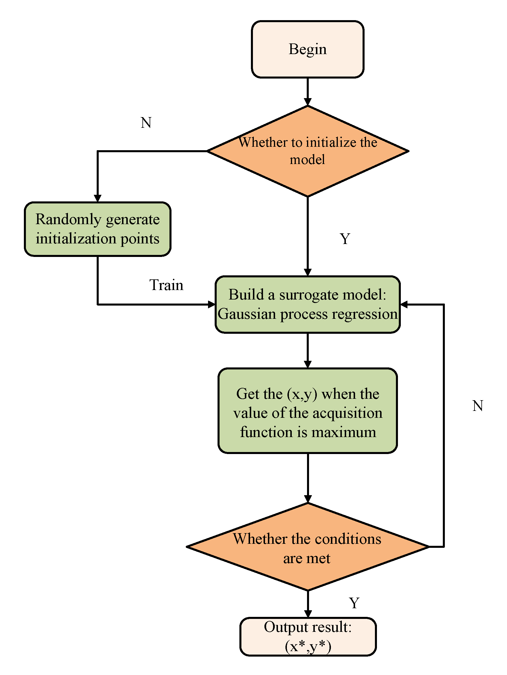
Bayesian optimization (BO) was first proposed by Pelikan, et al. of the University of Illinois Urbana-Champaign (UIUC) in 1998 [25]. It finds the optimal value of the function by constructing a posteriori probability of the output of the black box function when the limited sample points are known. Because the BO algorithm is very efficient, it is especially useful when the evaluation cost of the objective function is high, the derivative of the independent variable can not be obtained, or there are multiple peaks. BO method has two core components, one is a probabilistic surrogate model composed of prior distributions, and the other is the acquisition function. BO is a sequential model, and the posterior probability is updated by the new sample points in each iteration. At the same time, in order to avoid falling into the local optimal value, BO algorithms usually add some randomness to make a tradeoff between random exploration and a posteriori distribution. BO is one of the few hyper-parameter estimation methods with good convergence theory [26].
Taking the optimization of hyper-parameters of models with BO as the research direction, the problem of finding the global maximum or minimum value of black objective function is defined as (this paper takes finding the maximum value of objective function as an example):
where , X is hyper-parameters space. The purpose of this article is to find the maximum value of the objective function. Suppose the existing data is , is the generalization accuracy of the model under the hyper-parameter . In the following, was simplified as D. We hope to estimate the maximum value of the objective function in a limited number of iterations. If y is regarded as a random observation of the generalization accuracy, , where the noise satisfies , independent and identically distributed. The goal of hyper-parameter estimation is to find in the d-dimensional hyper-parameters space.
One problem with this maximum expected accuracy framework is that the true sequential accuracy is typically computationally intractable. This has led to the introduction of many myopic heuristics known as acquisition functions, which is maximized as:
There are three commonly acquisition functions: probability of improvement (PI), expected improvement (EI) and upper confidence bounds (UCB). These acquisition functions trade off exploration against exploitation.
2.2. Particle Swarm Optimization
Particle swarm optimization (PSO) [36,37] is a method based on swarm intelligence, which was first proposed by Kenndy and Eberhart in 1995 [38]. Because of its simplicity in implementation, PSO algorithm is successfully used in machine learning, signal processing, adaptive control and so on. The PSO algorithm first initializes m particles randomly, and each particle is a potential solution to the problem that needs to be solved in the search space.
In each iteration, the velocities and positions of each particle are updated using two values: one is the best value of particle, and the other is the best value of population overall previous. Suppose there are m particles in the d-dimensional search space, the velocity v and position x of the i-th particle at the time of t are expressed as:
The best value of particle and the overall previous best value of population at iteration t are:
At iteration , the position and velocity of the particle are updated as follows:
where is the inertia weight coefficient, which can trade off the global search ability against local search ability; and are the learning factors of the algorithm. If , it is easy to fall into and can not jump out local optimization; if , it will lead to slow convergence speed of PSO; and are random variables uniformly distributed in .
In each iteration of the PSO algorithm, only the optimal particle can transmit the information to other particles. The algorithm generally has two termination conditions: a maximum number of iterations or a sufficiently good fitness value.
2.3. Recurrent Neural Network
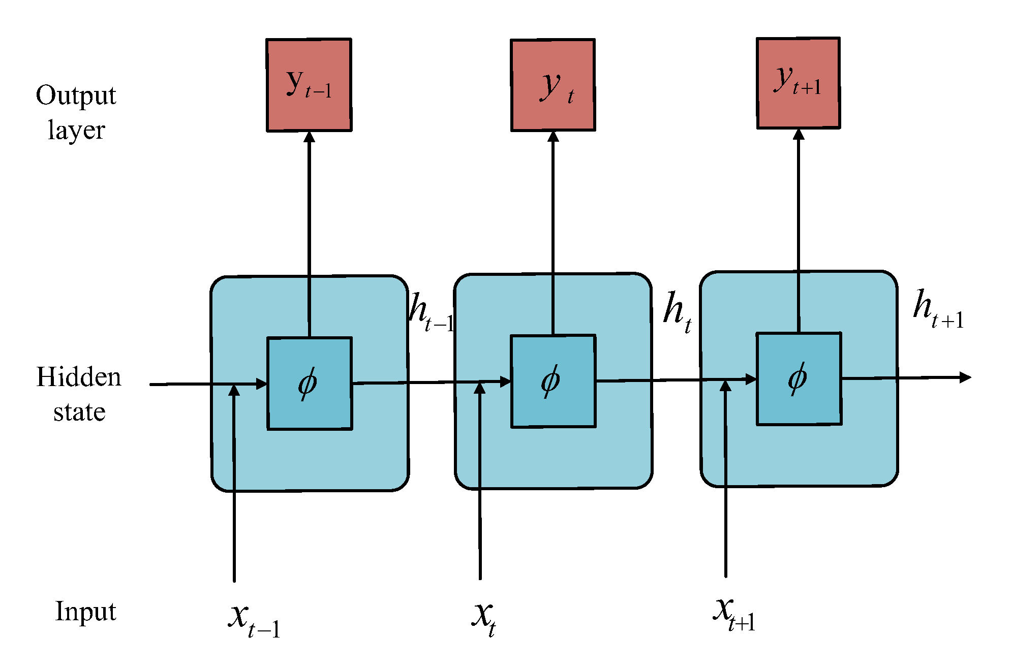
The recurrent neural network (RNN) does not rigidly memorize all fixed-length sequences. On the input sequence , it determines the output sequence by storing the hidden state of the time step information. The network structure is shown in Figure 2, where the calculation of is determined by the input of the current time step and the hidden variables of the previous time step:
where is the activation function, , are the weight, is the hidden layer deviation.
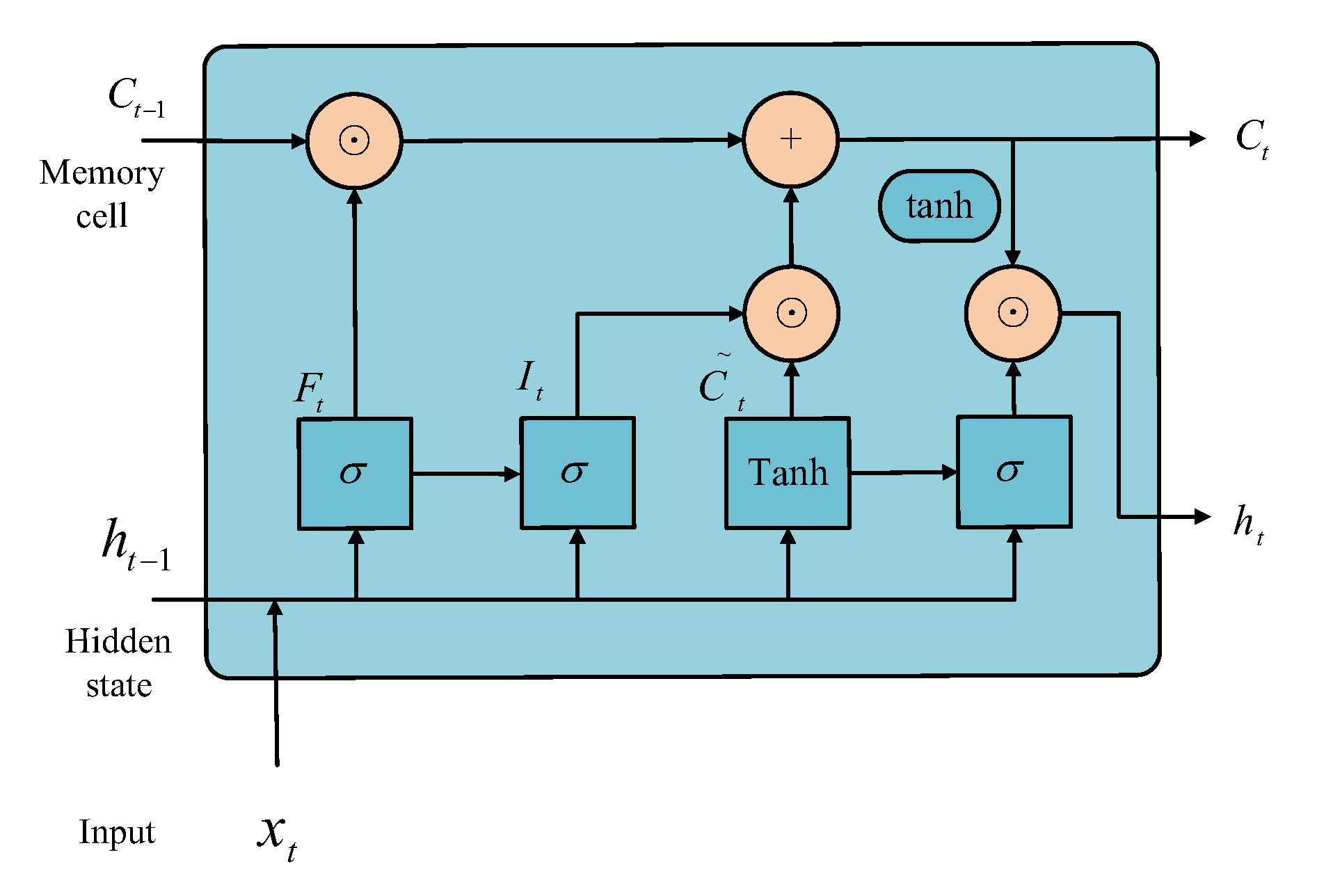
Long-Short term Memories (LSTM) is a kind of gated recurrent neural network, which is carefully designed to avoid long-term dependence. It introduces three gates on the basis of RNN, namely, input gate, forget gate and output gate, as well as memory cells with the same shape as the hidden state, so as to record additional information. As shown in the Figure 3, the input of the gate of LSTM is the current time step input, such as and the previous time step hidden state , and the output is calculated by the full connection layer. In this way, the values of the three gates are all in the range of . Suppose the number of hidden units is l, the input of time step t and the hidden state of the previous time step, memory cell , candidate memory cell , input gate , forget gate and output gate . The calculations are as follows:
where is the activation function, , , ,, , , , are the weight, ,,, are the hidden layer deviation. Once the memory cell is obtained, the flow of information from the memory cell to the hidden state can be controlled by output gate:
where the tanh function ensures that the hidden state element value is between and 1.
3. BO-PSO
BO algorithm based on particle swarm optimization (BO-PSO) is an iterative process. PSO is used to solve the maximum value of the acquisition function to obtain the next point to be evaluated; Then, the value of the objective function is evaluated according to ; Finally, the existing data D is updated with the new sample data , and the posterior distribution of the probabilistic surrogate model is updated to prepare for the next round of iteration.
3.1. Algorithm Framework
The effectiveness of BO depends on the acquisition function to some extent. The acquisition function generally has the characteristics of non-convex and multi-peak, which needs to solve the non-convex optimization problem in the search space X. PSO has the advantages of simplicity, few parameters need to be adjusted, fast convergence and so on. It is not necessary to calculate the derivative of the objective function. Therefore, this paper chooses PSO to optimize the acquisition function to obtain new sample points.
First, we need to select a surrogate model. The approximation characteristics of potential functions and the ability to measure uncertainty of Gaussian process (GP) make it a popular choice of surrogate model. Gaussian process is a nonparametric model determined by mean function and covariance function (positive definite kernel function). In general, every finite subset of the Gaussian process model follows the multi variable normal distribution. Assuming that the output expectation of the model is 0, the joint distribution of the existing data D and the new sample point can be expressed as follows:
The mathematical expectation and variance of are as follows:
The ability of GP to express the distribution of functions only depends on the covariance function. Matern-52 covariance function is one of them and as follows:
The second choice we need to make is acquisition function. Although our method is applicable to most acquisition functions, we choose to use UCB which is more popular in our experiment. GP-UCB proposed by Srinivas in 2009 [39]. The UCB strategy considers to increase the value of the confidence boundary on the surrogate model as much as possible, and its acquisition functions is as follows:
the is a parameter that controls the trade-off between exploration (visiting unexplored areas in X) and exploitation (refining our belief by querying close to previous samples). This parameter can be fixed to a constant value.
3.2. Algorithm Framework
BO-PSO consists of the following steps: (i) assume a surrogate model for the black box function f, (ii) define an acquisition function based on the surrogate model of f, and maximize by the PSO to decide the next evaluation point, (iii) observe the objective function at the point specified by maximization, and update the GP model using the observed data. BO-PSO algorithm repeats (ii) and (iii) above until it meets the stopping conditions. The Algorithm 1 framework is as follows:
| Algorithm 1 BO-PSO. |
| Input: surrogate model for f, acquisition function |
| Output: hyper-parameters vector optimal |
| Step 1. Initialize hyper-parameters vector ; |
| Step 2. For do: |
| Step 3. Using algorithm 1 to maximize the acquisition function to get the next evaluation point: ; |
| Step 4. Evaluation objective function value ; |
| Step 5. Update data: , and update the surrogate model; |
| Step 6. End for. |
4. Results
To verify the effectiveness of BO-PSO, we select the power load data set of a given year from the city of Nanchang, and determine the hyper-parameters of RNN and LSTM model based on the optimization method proposed in this paper to realize power load forecasting.
4.1. Data Sets and Setups
In this study, the power load data set includes 35,043 data, in which a sampling frequency is 15 min. The dataset was normalised to eliminate the magnitude differences. And the dataset was divided into a training set and a test set, with a test set size of 3000.
In the process of hyper-parameter optimization of machine learning model, when there are boundary restrictions of hyper-parameter in the BO, the methods to optimize the acquisition function are L-BFGS-B, TNC, SLSQP, TC and so on. Among them, L-BFGS-B and TNC are the most commonly used. We choose these two methods as the comparison methods, and the corresponding BO framework are named BO-L-BFGS-B and BO-TNC respectively.
The PSO algorithm can guarantee the convergence of the algorithm when the parameter satisfies the condition [40]. and affect the expected value and variance of the particle position. The smaller the variance is, the more concentrated the optimization result is, and the better the stability of the optimization system is. Other related research results show that the constant inertia and acceleration coefficient have good convergence characteristics [41], and the PSO parameters in this experiment are set according to this.
To ensure the comparability of the experiment, all the train and test are run in the same code package of Python; The surrogate model is a Gaussian process with mean function 0 and covariance function Matern-52, and the kernel function and hyper-parametric likelihood are optimized by maximizing logarithmic likelihood; The acquisition function is UCB, and optimization algorithm is randomly initialized with 5 observations in each experiment.
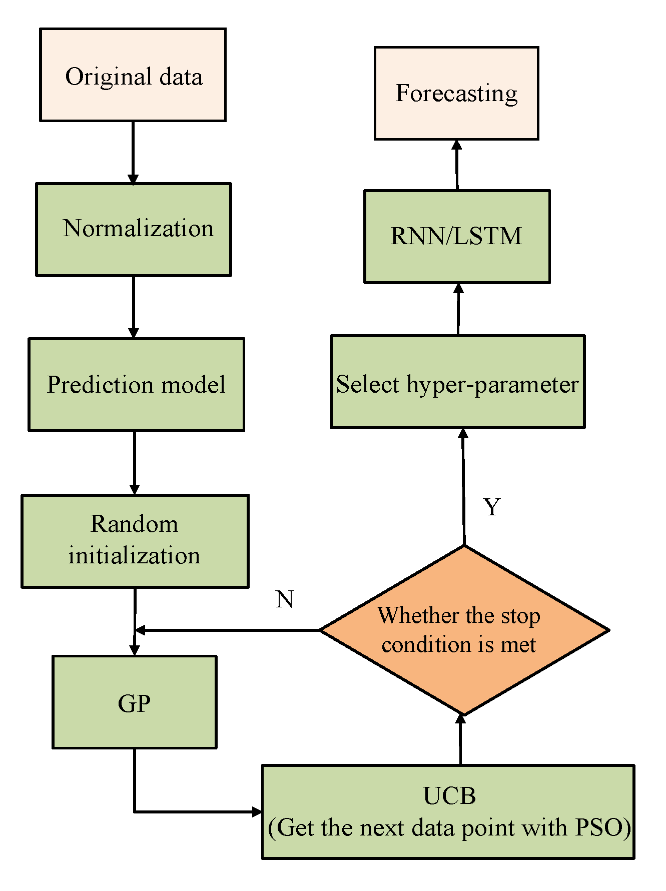
In this experiment, RNN and LSTM are selected as the basic model of power forecasting. The search space of hyper-parameters is shown in Table 1. The optimal hyper-parameters are selected by BO-PSO, BO-L-BFGS and BO- TNC algorithms, and the corresponding model are named RNN-BO-PSO, RNN-BO-L-BFGS-B, RNN-BO-TNC, LSTM-BO-PSO, LSTM-BO-L-BFGS-B and LSTM-BO-TNC respectively, with 50 iterations. Repeat training 10 times for each model independently to ensure the objectivity of the results. The training epochs for the RNN and LSTM models are 100. Based on the comprehensive analysis of the results, the hyper-parameter values of RNN and LSTM models are finally determined. The step flow of BO-PSO method to optimize hyper-parameters is shown in Figure 4.
4.2. Comparative Prediction Results
In order to compare the accuracy of several prediction models, the normalized mean square error (NMSE), the median square error (NMDSE) and coefficient of determination () are selected as the evaluation of the performance of hyper-parameters, the calculation formula is as follows:
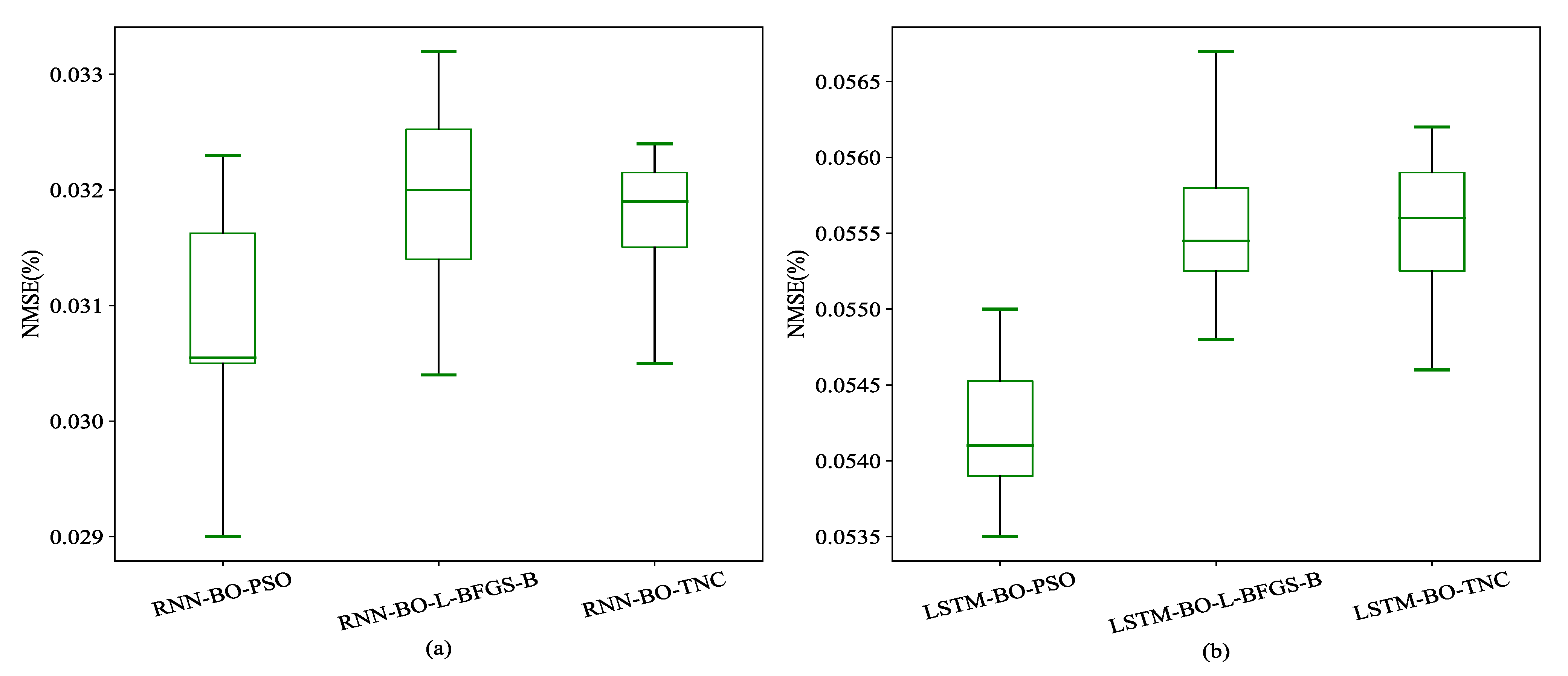
where is the actual power consumption at time t, is the predicted power consumption at time t. Finally, the values of in Table 2 of models are close to 1, which means that all of these models achieve an excellent fitting effect. BO-PSO performs better than others methods in the view of . A visual comparison of the values of NMSE is shown in Figure 5.
It can be seen that after optimizing the model, the NMSE value of the BO-PSO method, whether the maximum value, the minimum value or the average value, is smaller than that of the other two methods, which shows that the BO-PSO method is effective in this experiment and is better than the other two methods. After comparing the NMSE and values of the three methods, the final hyper-parameter (Feature length, Number of network units, Batch size of training data) values are shown in Table 3.
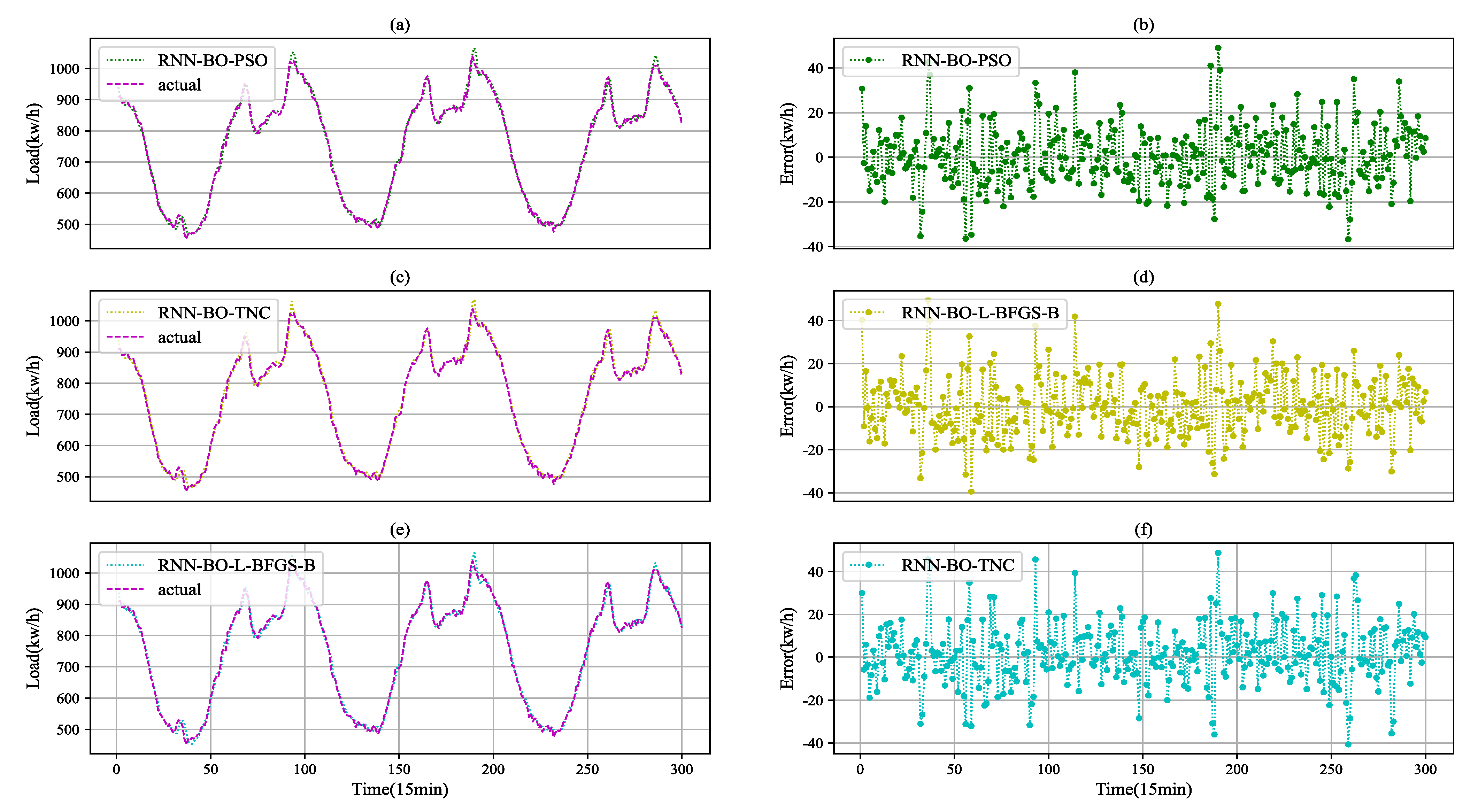
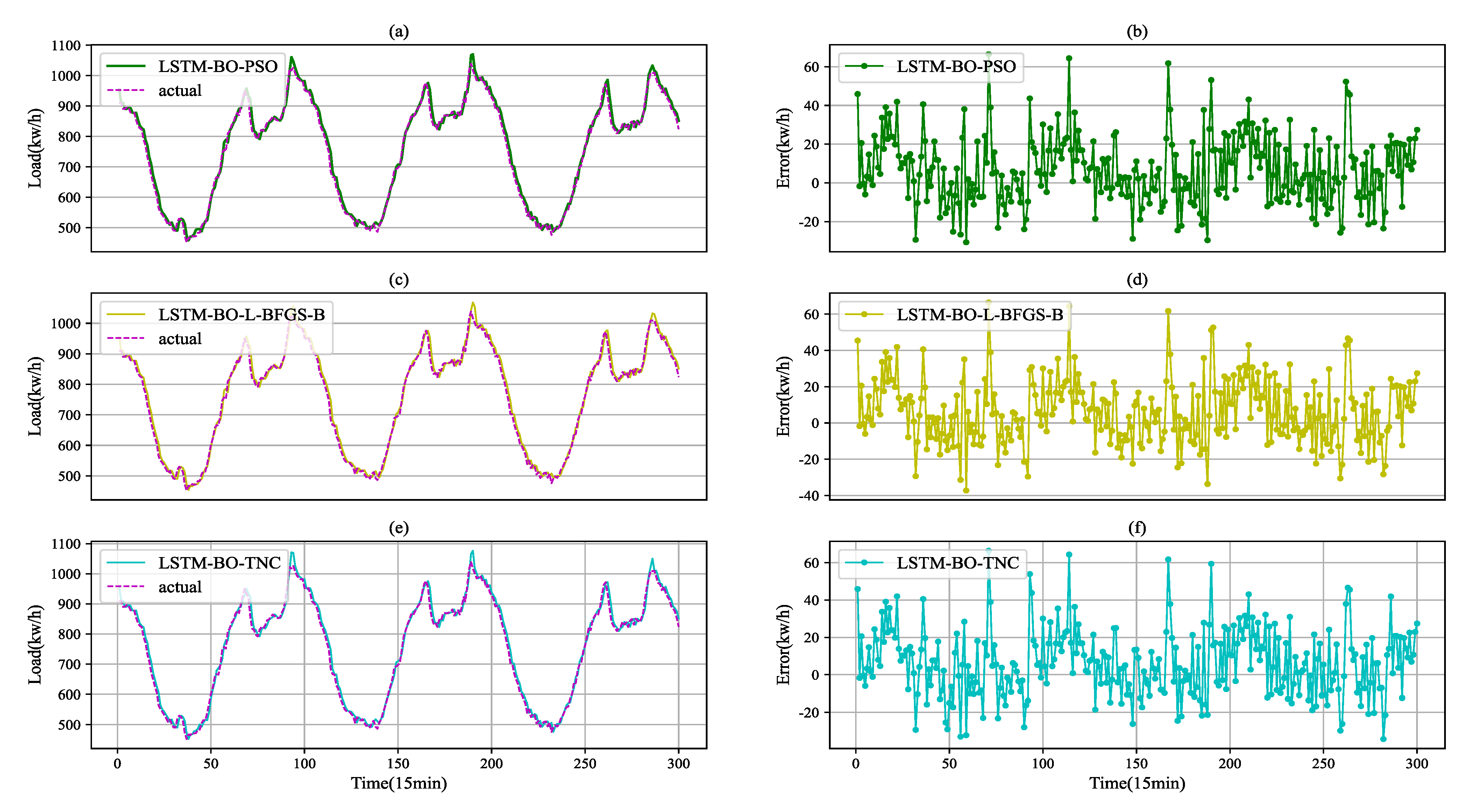
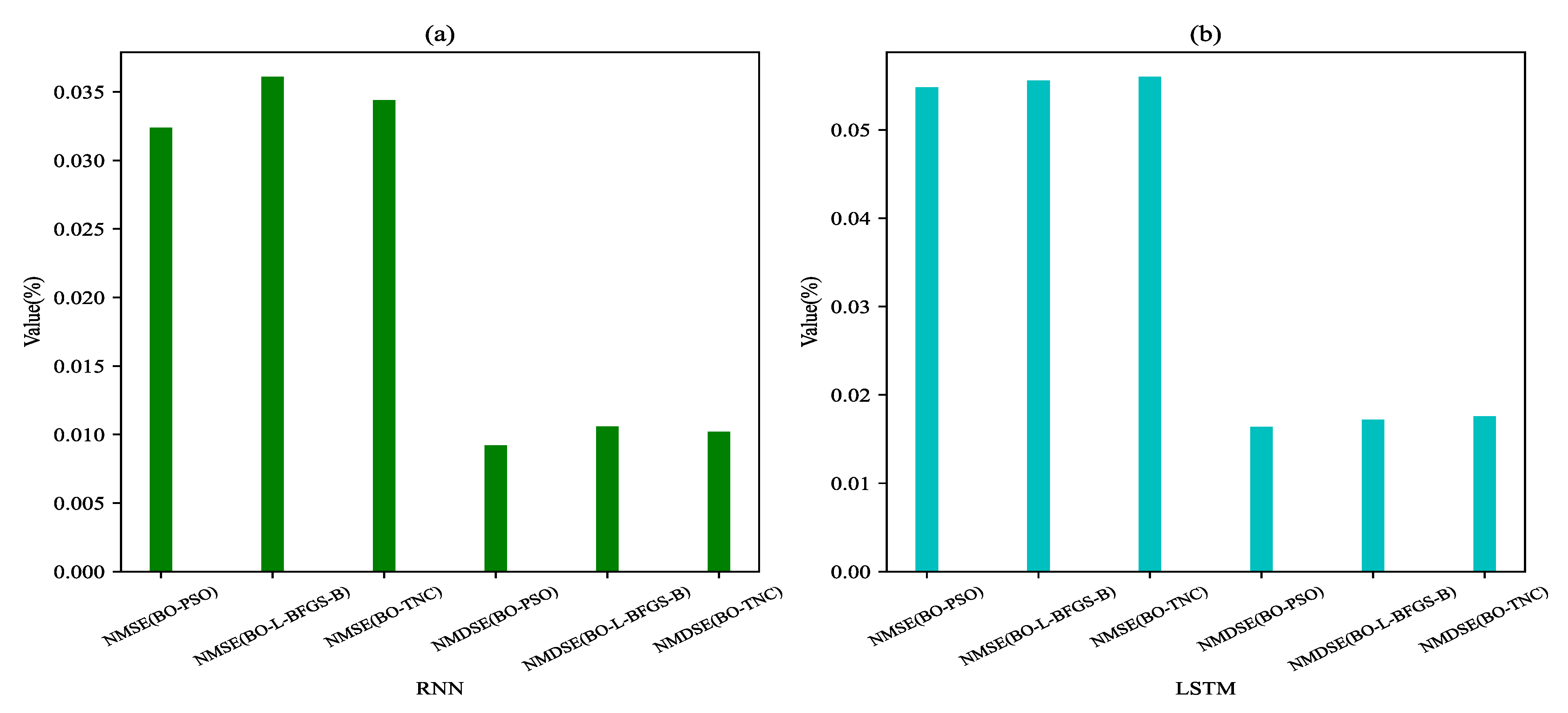
To show the comparison of the effects of the three methods more intuitively, the hyper-parameters in Table 3 are used to train the RNN and LSTM models. The top 300 predictions for the test set using the proposed method and the comparison method as shown in Figure 6 and Figure 7, it can be seen that there is an obvious fluctuation law of power load and the prediction results are closest to the true values. At the same time, the point-by-point prediction error of each model is shown. It can be observed that the prediction curves fit well for these six models. The error curves of RNN-BO-PSO and LSTM-BO-PSO fluctuate smoothly. The error of RNN-BO-PSO and LSTM-BO-PSO are obviously less than the other models in Figure 6 and Figure 7. After calculation, the NMSE value and NMDSE value of models are obtained, as shown in Table 4. Figure 8 shows the comparison of the two indicators, respectively. As can be seen from the chart, the two models optimized based on the BO-PSO method have the smallest NMSE and NMDSE. Thus, it can be seen that the optimization method in this paper can not only replace the manual selection of hyper-parameters, but also improve the performance of the model. From the results of Figure 6, Figure 7 and Figure 8 and Table 4, we can see that BO-PSO is an effective hyper-parameter optimization method.
5. Conclusions
Hyper-parameters have been a key problem in the practical application of machine learning models. In this paper, the BO-PSO algorithm is proposed, which gives full play to the simple calculation of PSO and high sample efficiency of BO for time series data modeling. In this method, the PSO algorithm is used to solve the maximum value of the acquisition function, to obtain new points to be evaluated, which solves the problem that the basic method needs to calculate the gradient and greatly reduces the computational complexity. Finally, we use BO-PSO to confirm the hyper-parameters of RNN and LSTM models, and compare the optimization results with BO-L-BFGS-B and BO-TNC methods. The errors of the prediction result in different models show that BO-PSO is an effective hyper-parameter optimization method, which can be applied to power load forecasting based on neural network model.
However, the algorithm has not been run in the high-dimensional space. In the future work, we plan to continue to improve the BO-PSO algorithm on this basis, so that it can also run effectively in high-dimensional space.
Author Contributions
Conceptualization, Y.Z.; methodology, Y.L. and Y.Z.; formal analysis, Y.L. and Y.Z.; writing—original draft preparation, Y.L. and Y.Z.; writing—review and editing, Y.L. and Y.C.; visualization, Y.L. and Y.C. All authors have read and agreed to the published version of the manuscript.
Funding
This research was funded by the Young Scientists Fund of the National Natural Science Foundation of China (grant numbers: 61803337).
Data Availability Statement
Not Applicable.
Acknowledgments
The author would like to thank the editors and anonymous reviewers for their suggestions to improve the quality of the paper.
Conflicts of Interest
The authors declare that there is no conflict of interest. The funders had no role in the design of the study; in the collection, analyses, or interpretation of data; in the writing of the manuscript; or in the decision to publish the results.
References
- Gülcü, A.; KUş, Z. Hyper-parameter selection in convolutional neural networks using microcanonical optimization algorithm. IEEE Access 2020, 8, 52528–52540. [Google Scholar] [CrossRef]
- Fan, S.K.S.; Hsu, C.Y.; Tsai, D.M.; He, F.; Cheng, C.C. Data-driven approach for fault detection and diagnostic in semiconductor manufacturing. IEEE Trans. Autom. Sci. Eng. 2020, 17, 1925–1936. [Google Scholar] [CrossRef]
- Fan, S.K.S.; Hsu, C.Y.; Jen, C.H.; Chen, K.L.; Juan, L.T. Defective wafer detection using a denoising autoencoder for semiconductor manufacturing processes. Adv. Eng. Inform. 2020, 46, 101166. [Google Scholar] [CrossRef]
- Park, Y.J.; Fan, S.K.S.; Hsu, C.Y. A Review on Fault Detection and Process Diagnostics in Industrial Processes. Processes 2020, 8, 1123. [Google Scholar] [CrossRef]
- Pu, L.; Zhang, X.L.; Wei, S.J.; Fan, X.T.; Xiong, Z.R. Target recognition of 3-d synthetic aperture radar images via deep belief network. In Proceedings of the CIE International Conference, Guangzhou, China, 10–13 October 2016. [Google Scholar]
- Wang, S.H.; Sun, J.D.; Phillips, P.; Zhao, G.H.; Zhang, Y.D. Polarimetric synthetic aperture radar image segmentation by convolutional neural network using graphical processing units. J. Real-Time Image Process. 2016, 15, 631–642. [Google Scholar] [CrossRef]
- Stoica, P.; Gershman, A.B. Maximum-likelihood DOA estimation by data-supported grid search. IEEE Signal Process. Lett. 1999, 6, 273–275. [Google Scholar] [CrossRef]
- Bellman, R.E. Adaptive Control Processes: A Guided Tour; Princeton University Press: Princeton, NJ, USA, 2015; pp. 1–5. [Google Scholar]
- Bergstra, J.; Bengio, Y. Random search for hyper-parameter optimization. J. Mach. Learn. Res. 2012, 13, 281–305. [Google Scholar]
- Frazier, P.I. A tutorial on Bayesian optimization. arXiv 2018, arXiv:1807.02811. [Google Scholar]
- Shahriari, B.; Swersky, K.; Wang, Z.Y.; Adams, R.P.; De Freitas, N. Taking the human out of the loop: A review of Bayesian optimization. Proc. IEEE 2015, 104, 148–175. [Google Scholar] [CrossRef] [Green Version]
- Cho, H.; Kim, Y.; Lee, E.; Choi, D.; Lee, Y.; Rhee, W. Basic enhancement strategies when using Bayesian optimization for hyperparameter tuning of deep neural networks. IEEE Access 2020, 8, 52588–52608. [Google Scholar] [CrossRef]
- Jones, D.R.; Schonlau, M.; Welch, W.J. Efficient global optimization of expensive black-box functions. J. Glob. Optim. 1998, 13, 455–492. [Google Scholar] [CrossRef]
- Liu, D.C.; Nocedal, J. On the limited memory BFGS method for large scale optimization. Math. Program. 1989, 45, 503–528. [Google Scholar] [CrossRef] [Green Version]
- Nash, S.G. A survey of truncated-Newton methods. J. Comput. Appl. Math. 2000, 124, 45–59. [Google Scholar] [CrossRef] [Green Version]
- Bai, Q.H. Analysis of particle swarm optimization algorithm. Comput. Inf. Sci. 2010, 3, 180. [Google Scholar] [CrossRef] [Green Version]
- Regulski, P.; Vilchis-Rodriguez, D.S.; Djurović, S.; Terzija, V. Estimation of composite load model parameters using an improved particle swarm optimization method. IEEE Trans. Power Deliv. 2014, 30, 553–560. [Google Scholar] [CrossRef]
- Schwaab, M.; Biscaia, E.C., Jr.; Monteiro, J.L.; Pinto, J.C. Nonlinear parameter estimation through particle swarm optimization. Chem. Eng. Sci. 2008, 63, 1542–1552. [Google Scholar] [CrossRef]
- Wenjing, Z. Parameter identification of LuGre friction model in servo system based on improved particle swarm optimization algorithm. In Proceedings of the Chinese Control Conference, Zhangjiajie, China, 26–31 July 2007. [Google Scholar]
- Bergstra, J.; Bardenet, R.; Bengio, Y.; Kégl, B. Algorithms for hyper-parameter optimization. In Proceedings of the Neural Information Processing Systems Foundation, Granada, Spain, 20 November 2011. [Google Scholar]
- Krajsek, K.; Mester, R. Marginalized Maximum a Posteriori Hyper-parameter Estimation for Global Optical Flow Techniques. In Proceedings of the American Institute of Physics Conference, Paris, France, 8–13 July 2006. [Google Scholar]
- Fumo, N.; Biswas, M.R. Regression analysis for prediction of residential energy consumption. Renew. Sustain. Energy Rev. 2015, 47, 332–343. [Google Scholar] [CrossRef]
- Liao, Z.; Gai, N.; Stansby, P.; Li, G. Linear non-causal optimal control of an attenuator type wave energy converter m4. IEEE Trans. Sustain. Energy 2019, 11, 1278–1286. [Google Scholar] [CrossRef] [Green Version]
- Zhuang, S.J. Cross-scale recurrent neural network based on Zoneout and its application in short-term power load forecasting. Comput. Sci. 2020, 47, 105–109. [Google Scholar]
- Snoek, J.; Larochelle, H.; Adams, R.P. Practical bayesian optimization of machine learning algorithms. arXiv 2012, arXiv:1206.2944. [Google Scholar]
- Brochu, E.; Cora, V.M.; De Freitas, N. A tutorial on Bayesian optimization of expensive cost functions, with application to active user modeling and hierarchical reinforcement learning. arXiv 2010, arXiv:1012.2599. [Google Scholar]
- Rasmussen, C.E. Gaussian processes in machine learning. In Summer School on Machine Learning; Springer: Berlin/Heidelberg, Germany, February 2003. [Google Scholar]
- Mahendran, N.; Wang, Z.; Hamze, F.; De Freitas, N. Adaptive MCMC with Bayesian optimization. In Proceedings of the Artificial Intelligence and Statistics, La Palma, Canary Islands, Spain, 21–23 April 2012. [Google Scholar]
- Hennig, P.; Schuler, C.J. Entropy Search for Information-Efficient Global Optimization. J. Mach. Learn. Res. 2012, 13, 1809–1837. [Google Scholar]
- Toscano-Palmerin, S.; Frazier, P.I. Bayesian optimization with expensive integrands. arXiv 2018, arXiv:1803.08661. [Google Scholar]
- Garrido-Merchán, E.C.; Hernández-Lobato, D. Dealing with categorical and integer-valued variables in bayesian optimization with gaussian processes. Neurocomputing 2020, 380, 20–35. [Google Scholar] [CrossRef] [Green Version]
- Oh, C.; Tomczak, J.M.; Gavves, E.M. Combinatorial bayesian optimization using the graph cartesian product. arXiv 2019, arXiv:1902.00448. [Google Scholar]
- Dai, Z.; Yu, H.; Low, B.K.H.; Jaillet, P. Bayesian optimization meets Bayesian optimal stopping. In Proceedings of the PMLR, Long Beach, CA, USA, 9–15 June 2019. [Google Scholar]
- Gong, C.; Peng, J.; Liu, Q. Quantile stein variational gradient descent for batch bayesian optimization. In Proceedings of the PMLR, Long Beach, CA, USA, 9–15 June 2019. [Google Scholar]
- Paria, B.; Kandasamy, K.; Póczos, B. A flexible framework for multi-objective Bayesian optimization using random scalarizations. In Proceedings of the PMLR, Toronto, AB, Canada, 3–6 August 2020. [Google Scholar]
- Fan, S.K.S.; Jen, C.H. An enhanced partial search to particle swarm optimization for unconstrained optimization. Mathematics 2019, 7, 357. [Google Scholar] [CrossRef] [Green Version]
- Fan, S.K.S.; Zahara, E. A hybrid simplex search and particle swarm optimization for unconstrained optimization. Eur. J. Oper. Res. 2007, 181, 527–548. [Google Scholar] [CrossRef]
- Hung, C.; Wan, L. Hybridization of particle swarm optimization with the k-means algorithm for image classification. In Proceedings of the 2009 IEEE Symposium on Computational Intelligence for Image Processing, Nashville, TN, USA, 30 March–2 April 2009. [Google Scholar]
- Srinivas, N.; Krause, A.; Kakade, S.M.; Seeger, M. Gaussian process optimization in the bandit setting: No regret and experimental design. arXiv 2009, arXiv:0912.3995. [Google Scholar]
- Jiang, M.; Luo, Y.P.; Yang, S.Y. Stochastic convergence analysis and parameter selection of the standard particle swarm optimization algorithm. Inf. Process. Lett. 2007, 102, 8–16. [Google Scholar] [CrossRef]
- Zheng, Y.; Ma, L.; Zhang, L.; Qian, J. On the convergence analysis and parameter selection in particle swarm optimization. In Proceedings of the 2003 International Conference on Machine Learning and Cybernetics (IEEE Cat. No. 03EX693), Xi’an, China, 5 November 2003. [Google Scholar]
Figure 1.
Flow chart of Bayesian optimization.

Figure 2.
Structure of RNN.

Figure 3.
Structure of LSTM.

Figure 4.
Flow chart of load forecasting.

Figure 5.
NMSE box line diagram for different models. (a) Value of NMSE of RNN models for each method. (b) Value of NMSE of LSTM models for each method.
Figure 5.
NMSE box line diagram for different models. (a) Value of NMSE of RNN models for each method. (b) Value of NMSE of LSTM models for each method.

Figure 6.
Load prediction for RNN. (a,c,e) The load fitting curves for RNN. (b,d,f) The load prediction error curves for RNN, which are obtained by subtracting the measured values from the predicted values. And the error curves correspond to the left fitting curves respectively.
Figure 6.
Load prediction for RNN. (a,c,e) The load fitting curves for RNN. (b,d,f) The load prediction error curves for RNN, which are obtained by subtracting the measured values from the predicted values. And the error curves correspond to the left fitting curves respectively.

Figure 7.
Load prediction for LSTM. (a,c,e) The load fitting curves for LSTM. (b,d,f) The load prediction error curves for LSTM, which are obtained by subtracting the measured values from the predicted values. And the error curves correspond to the left fitting curves respectively.
Figure 7.
Load prediction for LSTM. (a,c,e) The load fitting curves for LSTM. (b,d,f) The load prediction error curves for LSTM, which are obtained by subtracting the measured values from the predicted values. And the error curves correspond to the left fitting curves respectively.

Figure 8.
Comparison of values of NMSE and NMDSE. (a) Values of NMSE and NMDSE of RNN models optimized with the BO-PSO, BO-L-BFGS-B and BO-TNC (b) Values of NMSE and NMDSE of LSTM models optimized with the BO-PSO, BO-L-BFGS-B and BO-TNC.
Figure 8.
Comparison of values of NMSE and NMDSE. (a) Values of NMSE and NMDSE of RNN models optimized with the BO-PSO, BO-L-BFGS-B and BO-TNC (b) Values of NMSE and NMDSE of LSTM models optimized with the BO-PSO, BO-L-BFGS-B and BO-TNC.


Table 1.
Type and range of hyper-parameters.
| Hyper-Parameters | Type | Range |
|---|---|---|
| Feature length | Integer | (5, 50) |
| Number of network units | Integer | (5, 50) |
| Batch size of training data | Integer | (32, 4096) |
Table 2.
The value of for different models.
| Model | |
|---|---|
| RNN-BO-PSO | 0.9909 |
| RNN-BO-L-BFGS-B | 0.9908 |
| RNN-BO-TNC | 0.9907 |
| LSTM-BO-PSO | 0.9951 |
| LSTM-BO-L-BFGS-B | 0.9945 |
| LSTM-BO-TNC | 0.9948 |
Table 3.
The hyper-parameters of each network.
| Model | Feature Length | Number of Network Units | Batch Size of Training Data |
|---|---|---|---|
| RNN-BO-L-BFGS-B | 44 | 34 | 64 |
| RNN-BO-TNC | 49 | 34 | 64 |
| RNN-BO-PSO | 47 | 38 | 64 |
| LSTM-BO-L-BFGS-B | 23 | 33 | 64 |
| LSTM-BO-TNC | 23 | 32 | 64 |
| LSTM-BO-PSO | 45 | 38 | 32 |
Table 4.
Error of the prediction result in different models.
| Model | NMSE (%) | NMDSE (%) |
|---|---|---|
| RNN-BO-L-BFGS-B | 0.0361 | 0.0106 |
| RNN-BO-TNC | 0.0344 | 0.0102 |
| RNN-BO-PSO | 0.0324 | 0.0092 |
| LSTM-BO-L-BFGS-B | 0.0549 | 0.0172 |
| LSTM-BO-TNC | 0.0560 | 0.0177 |
| LSTM-BO-PSO | 0.0556 | 0.0164 |
Publisher’s Note: MDPI stays neutral with regard to jurisdictional claims in published maps and institutional affiliations. |
© 2021 by the authors. Licensee MDPI, Basel, Switzerland. This article is an open access article distributed under the terms and conditions of the Creative Commons Attribution (CC BY) license (https://creativecommons.org/licenses/by/4.0/).
Share and Cite
MDPI and ACS Style
Li, Y.; Zhang, Y.; Cai, Y. A New Hyper-Parameter Optimization Method for Power Load Forecast Based on Recurrent Neural Networks. Algorithms 2021, 14, 163. https://0-doi-org.brum.beds.ac.uk/10.3390/a14060163
AMA Style
Li Y, Zhang Y, Cai Y. A New Hyper-Parameter Optimization Method for Power Load Forecast Based on Recurrent Neural Networks. Algorithms. 2021; 14(6):163. https://0-doi-org.brum.beds.ac.uk/10.3390/a14060163
Chicago/Turabian StyleLi, Yaru, Yulai Zhang, and Yongping Cai. 2021. "A New Hyper-Parameter Optimization Method for Power Load Forecast Based on Recurrent Neural Networks" Algorithms 14, no. 6: 163. https://0-doi-org.brum.beds.ac.uk/10.3390/a14060163
Note that from the first issue of 2016, this journal uses article numbers instead of page numbers. See further details here.