1. Introduction
Let
be a (nonlinear) mapping and let
be the corresponding system of equations. In [
1], Xu proposed the following partially asynchronous block quasi-Newton method for such a nonlinear system. Let
be a partition of
F and
x in
p partitions,
,
, where
and
are block functions and block variables, respectively, of the same dimensions
. The variable
x is the common memory of the multiprocessor system, every processor
i can read the content of
x and can write its new update of
. Let
,
, be square matrices of dimension
. The main steps of the process
i are :
| Algorithm 1. |
| Input: |
| Output: x |
| 1. Compute |
| 2. Get from x by replacing with |
| 3. Compute and |
| 4. Update ; |
| 5. |
Applying the Sherman–Morrison lemma (Step 4, Algorithm 1) to inverse the matrix , the polynomial complexity of order three is reduced to polynomial complexity of order two.
More recently, in [
2,
3] Jiang and Yang proposed several preconditioners for the block Broyden’s method and discussed the implementation process. The main steps of parallel variant of Broyden’s method considered in [
2,
3] (Algorithm 2 below) are (
is a block diagonal matrix,
is the
diagonal block of
):
| Algorithm 2. |
| Input: |
| Output: |
| 1. For Until Or Do |
| 2. ; |
| 3. ; |
| 4. For |
| 5. . |
| 6. End |
| 7. End |
In the case of a linear system, the sequential Broyden’s method has global convergence provided that the system matrix is invertible [
4],
i.e., the sequence generated by this method converges to the solution of the system for any starting point
and for any starting matrix
(or
). Moreover, in this case the convergence is finite [
5], and the solution is obtained in at most
steps; conditions in which this method requires a full
steps to converge are also given. In the same paper [
5], it is shown that Broyden’s method has
-step Q-quadratic local convergence for the nonlinear case (the initial starting point
and the initial starting matrix
must be close to the solution point of the system and to the Jacobian matrix in the solution point, respectively). Note that
-step Q-quadratic convergence means that the subsequence
of
has Q-quadratic convergence.
In this paper we propose some new variants of parallel Broyden’s method that are suitable both for linear and nonlinear systems. We prove the convergence of our basic algorithm in the linear case. Numerical experiments are presented for linear and nonlinear cases, and some remarks are made concerning the behavior of the generated sequence.
2. The Parallel Variants and Preliminaries
In the case of a linear mapping,
, the Broyden’s “good formula” [
6,
7],
(
B and
are the current and the next iterates, respectively, and
θ is a positive number chosen such that
is invertible [
4]) can be written in the following form:
. Using the notation
, the Broyden’s method becomes
. The main idea of the proposed variants is to use instead of
A the block diagonal matrix of
A, denoted by
D throughout the paper, partitioned according to
. The computer routine
will produce such a block diagonal matrix,
i.e.,
.
Based on this idea we can consider several parallel variants of Broyden’s algorithm. The first variant is just the above mentioned algorithm, to which we added a supplementary step to successively block-diagonalize the matrix
E (the Step 5, Algorithm 3 below). We consider also the following slight modification of update formula
By adding
D to both sides of this formula, the algorithm becomes more homogeneous (the same matrix is used in both Steps 2 and 4, Algorithm 3 below). Moreover (and not in the least) for this variant, a simple and elegant proof can be given for the convergence of the generated sequence (Theorem 1). Therefore the first our variant, which will be considered as the basic algorithm, is (
is a block diagonal matrix):
| Algorithm 3. |
| Input: |
| Output: |
| 1: For Until Or Do |
| 2: |
| 3: |
| 4: |
| 5: |
| 6. End |
A variant of Algorithm 3 can be obtained by applying the Sherman–Morrison lemma to avoid the inversion of a matrix in Step 2. It results the following Algorithm 4 (
is a block diagonal matrix):
| Algorithm 4. |
| Input: |
| Output: |
| 1: For Until Or Do |
| 2: |
| 3: |
| 4: ): |
| 5: |
| 6. End |
The simplest way to design a similar parallel algorithm for the nonlinear case is to replace
D in the basic algorithm with the diagonal block of the Jacobian of
F,
. It results the following Algorithm 5 for the nonlinear case:
| Algorithm 5. |
| Input: |
| Output: |
| 1: For Until Or Do |
| 2: |
| 3: |
| 4: |
| 5: |
| 6. End |
Remark 1. The formal replacement of D with is based on the mean value theorem . However, the convergence properties of Algorithm 5, including its specific conditions, rate of convergence, etc.,
must be further analyzed as well. The numerical experiments (Section 5) performed so far for certain nonlinear systems show a comparable behavior of the two Algorithms (3 and 5) for the linear and nonlinear case. The main processing of the Algorithms 3, 5, is the computation of or the solution of a corresponding linear system. Taking into account that is a block diagonal matrix, , where , , are matrices of dimension , we have to perform p subtasks, whose main processing is . It is obvious that these subtasks can be done in parallel. The successive updates of the matrix E, Steps 4 and 5, can also be executed in parallel. The concrete parallel implementation of this algorithm is an interesting problem and is left for a future research.
As usual denotes the set of square real matrices. We use and to denote the spectral and Frobenius norm respectively. The properties of Algorithm 3 are based on the following two lemmas.
Lemma 1. Let be a block diagonal matrix (conforming with ). Then, for any matrix , there holdswhere is the spectral or Frobenius norm. If then the sequence as defined in Algorithm 3 is bounded, .
Proof. Using the inequality
(which is true for both spectral and Frobenius norm), we have
To prove the second part of Lemma 1, observe that if
then
for any
. Therefore
Thus
and
is bounded. ☐
Lemma 2. For any matrix , any , any , and we have (The Formula (1) appears also in [
4]; a short proof is given here for completeness).
Proof. By trivial computation we obtain
.
Use , , and the desired equality results. ☐
3. The Convergence of Algorithm 3 in the Linear Case
In the following, we suppose that the sequence
given by Algorithm 3, with starting point
, starting matrix
and certain
θ, satisfies the condition:
Algorithm 3 defines the next iteration as a function of the current iteration,
,
G being the iteration function or generation function. It is clear that the condition (2) is weaker than the condition of asymptotic regularity of
G or asymptotic regularity of
under G, (
). The fulfillment of condition (2) depends not only on the characteristics of
A (like the condition number) but also on
and
θ. Note also that usually, the sequence
is bounded, and if
F is also bounded on
then the condition (2) is satisfied; in
Section 5 an example of mapping is given which is bounded on
and
.
Theorem 1. Let be a nonsingular matrix, , and let θ be a real number, . Suppose that D is invertible and that , where a is defined in Lemma 1. Suppose also that condition (2) is satisfied and that is invertible. Then the parallel variant of Broyden method (Algorithm 3) converges to the solution of the equation .
Proof. Since
, from perturbation Lemma, it results that
exists for all
n and the sequence
is well defined by Algorithm 3. By taking
and applying Lemmas 1 and 2, we obtain
By summing on
k,
, we have
Now, because
, we have
and
☐
4. Remarks on the Parallel Implementation
The parallelization of the product (Step 2 in Algorithm 3) is obvious, because is block diagonal. Concerning the product , observe first that the element of the product is and can be computed by a very simple algorithm. Then, because is block diagonal, with dimensions , the product gives the lines of . These products are independent from each other and therefore can be computed in parallel. The same observations can be made for Algorithms 4 and 5.
In order to implement this method, let us suppose that the multiprocessor system has
p processors. A simple idea is to set the system into
p partitions and assign a partition to every processor. In this case the following issue arises: How large should the partitions
be in order to obtain a low cumulative computation cost per iteration? In the case of Algorithms 3 and 5, the main processing of processor
i is to inverse a matrix of dimension
. Therefore every processor has to perform a computation that has a polynomial complexity of order
. The cumulative computation cost for all
p processors is
, and, if there is not overlapping,
. Further, we use the following elementary inequality
where
are positive numbers and
. If
and
, then
We will prove now that if
then
Because , it is sufficient to show that , and this is equivalent with the first part of (3). We obtain the following
Propositon 1. Suppose that the smallest size of partitions, , satisfies the condition (3). Then the cumulative computation cost in Algorithms 3 and 5 is less than .
A similar result can be established for Algorithm 4. The condition (3) becomes
and the cumulative computation cost satisfies
.
5. Numerical Experiments and Conclusions
The main purpose of this section is to highlight the convergence properties of the proposed parallel Broyden’s algorithms in the case of a synchronous model. The communication costs between processors, scheduling and loads balancing, optimal processors assignment, and so on, both for synchronous and asynchronous models, are important issues in themselves. However they are not the subject of the present study.
The behavior of the sequence
obtained by the proposed algorithms and for various linear or nonlinear cases is shown in our experiments by the graph of
, where
is the error at step
n,
or
(
n on horizontal axis and
on vertical axis). The convergence of the process entails a decreasing graph until negative values (for example,
means
). If the convergence is linear (
) then
;
depends linearly on
n and the graph of
is close to a straight line. For comparison reasons, the proposed parallel Broyden’s method is compared with the parallel Newton method and the parallel Cimmino method. We consider the following parallel Newton method [
8]:
where
is the Jacobian of
F. Note that in the case of a linear system, by applying this form of Newton method, the direct computation of
(in one iteration) is lost and the convergence is linear. Consequently, the graph of
is a straight line.
The block Cimmino method is considered only for the linear case,
, and it can be described as follows (see, for example, [
9]). The system is partitioned into
p strips of rows,
and
,
. Supposing that
has full row rank, the Moore–Penrose pseudo inverse of
is defined by
. The block Cimmino algorithm is
Step 1: Compute in parallel
Step 2:
where
ω is a relaxation parameter.
Experiment 1.
We applied Algorithm 3 to linear systems of medium dimensions, , with different values of condition numbers. A program “genA” generates a square, sparse matrix A of dimension m with random elements and , where are given (positive) numbers. The percent of nonzero elements is an entry data of “genA” and in this experiment we considered it to be about 50%. The free term b and the starting point were also randomly generated with elements between some limits. Thus the function F is randomly defined by .
Figure 1.
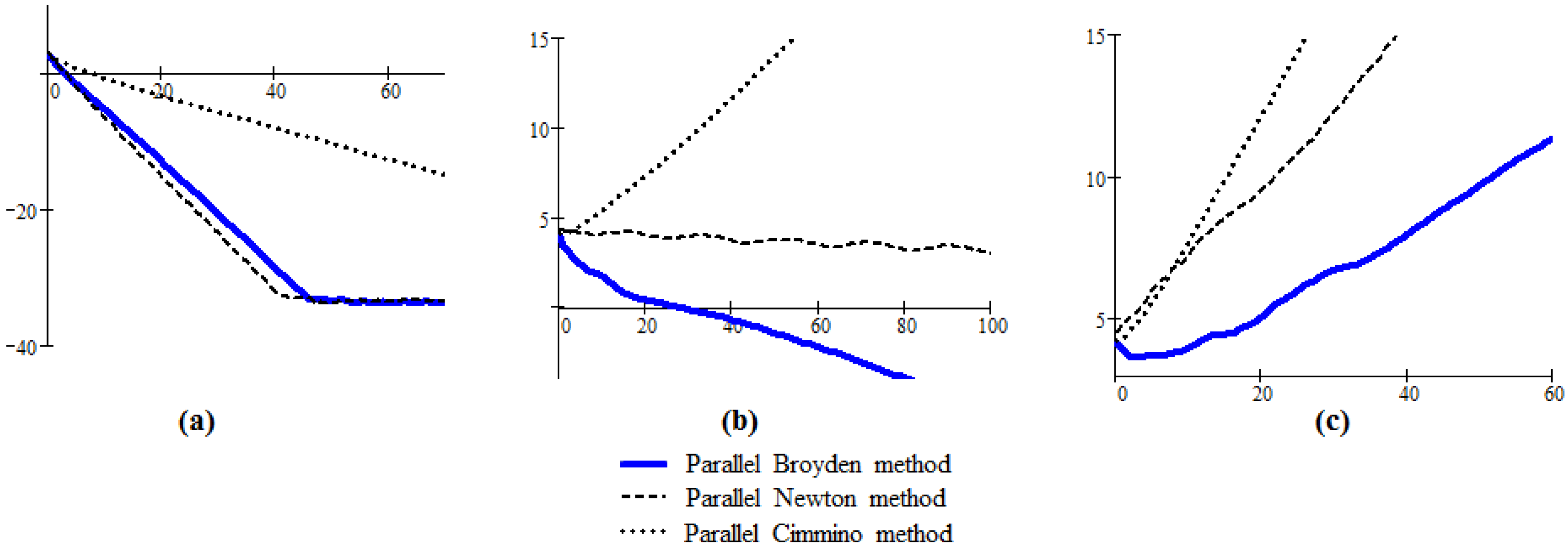
The graphs of generated by Algorithm 3, parallel Newton method and parallel Cimmino method in the linear case; (a) system well conditioned; (b) system medium conditioned; (c) system poorly conditioned.
Figure 1.
The graphs of generated by Algorithm 3, parallel Newton method and parallel Cimmino method in the linear case; (a) system well conditioned; (b) system medium conditioned; (c) system poorly conditioned.
For every considered system, we applied Algorithm 3, the parallel Newton method and the parallel Cimmino method, and we drew the resulting graphs in the same plot; for the graph of Algorithm 3 we used a continuous line, for the parallel Newton method a dashed line, and for the parallel Cimmino method a dotted line. The number of partitions and the dimensions of every partition are entry data of the routine “diag(A)”. The test systems were automatically generated by routine “genA"; the three graphs of
Figure 1 are examples from a large number of cases, corresponding to certain systems of dimensions 50, 100, 200 respectively; other parameters like
c (the condition number),
θ (the factor in Step 4),
(the number of partitions and their dimensions), were chosen as follows:
- (a)
,
- (b)
,
- (c)
.
The following conclusions can be drawn. (1) The proposed parallel Broyden’s algorithm works well if the system is relatively well conditioned (the condition number should be around ten), and in this case the behavior of Algorithm 3 is very similar to the parallel Newton method and significantly better than the parallel Cimmino method. (
Figure 1a); (2) For medium conditioned systems, the behavior of Algorithm 3 is unpredictable, sometimes it works better than the Newton method (
Figure 1b); (3) If the system is poorly conditioned (the condition number is greater than 300) the proposed parallel Broyden’s algorithm fails to converge (the Newton method has the same behavior) (
Figure 1c).
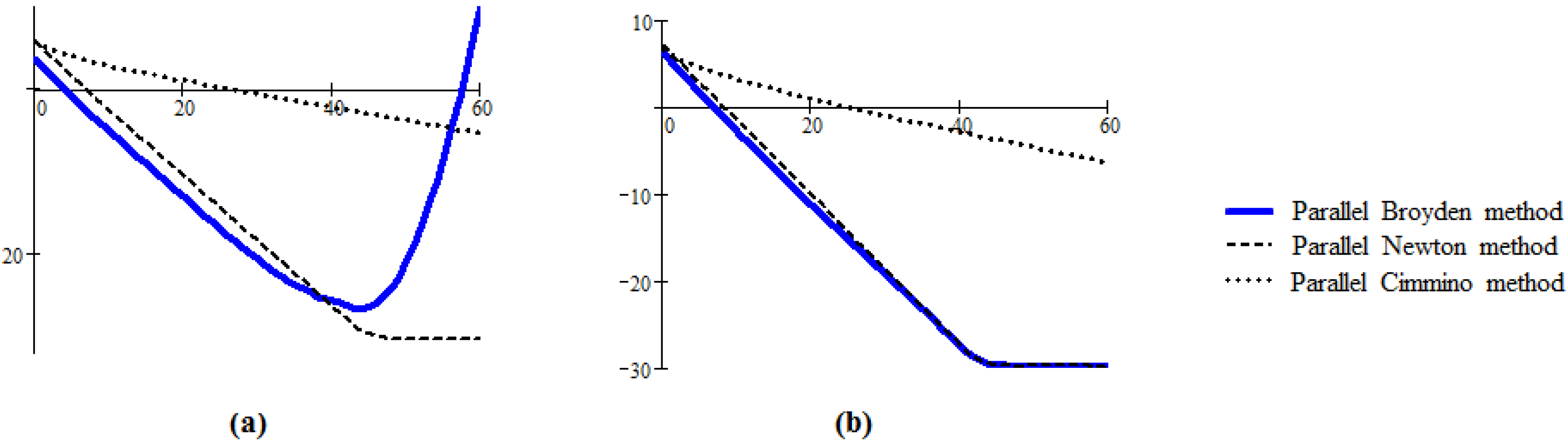
Figure 2a presents the behavior of the sequence generated by the Algorithm 3 for a linear system of dimension
,
. The condition (2) of Theorem 1 is not satisfied and the sequence generated by this algorithm (in this case) does not converge. However, the behavior is interesting, the generated sequence becomes very close to the solution, the error decreases until a very small value (in our example until
), and then the good behavior is broken. The graph corresponding to the sequence generated by Algorithm 4 for a system of dimension
and
is presented in
Figure 2b. We can observe the similarities between this sequence and the sequence obtained by the parallel Newton method.
Figure 2.
The behavior of the sequence generated by Algorithm 3, Parallel Newton method and Parallel Cimmino method (the graphs (a)) and by Algorithm 4, Parallel Newton method and Parallel Cimmino method (the graphs (b)); (a) system which does not satisfy the condition (2); (b) system well conditioned.
Remark 2. The numerical experiments presented here, for the most part, have been performed with the basic Algorithm 3; for Algorithm 4 similar conclusions can be drawn. A special characteristics of Algorithm 4, in comparison with Algorithm 3, is that Algorithm 4 is less sensitive to θ; this parameter can take its values on a much larger interval, .
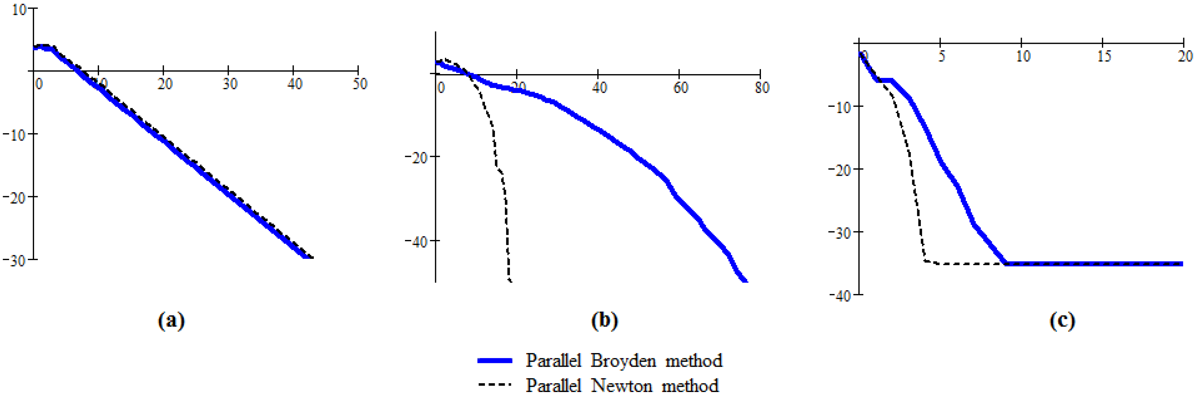
Experiment 2.
This experiment is devoted to show the behavior of the sequences generated by Algorithm 5 in the case of nonlinear systems. We considered several nonlinear systems of low dimensions and of certain sparsity (every nonlinear equation depends on a few numbers of unknowns).
Figure 3 presents the results for the following three nonlinear systems:
Figure 3.
The graphs of generated by Algorithm 5 and parallel Newton method; (a) the graph corresponding to systems (1); (b) the graph corresponding to systems (2) given by Algorithm 5 modified in accordance with Sherman-Morrison lemma; (c) example of a system verifying the condition .
Figure 3.
The graphs of generated by Algorithm 5 and parallel Newton method; (a) the graph corresponding to systems (1); (b) the graph corresponding to systems (2) given by Algorithm 5 modified in accordance with Sherman-Morrison lemma; (c) example of a system verifying the condition .
The proposed parallel Broyden’s method is compared with the parallel Newton method described above. The conclusion is that, generally, the parallel Broyden’s method has similar characteristics with the considered parallel Newton method, convergence properties, attraction basin,
etc. This similarity can be seen in the case of the first system (
Figure 3a). The third system is an example for which
F is bounded on
, as it is required in
Section 3. Note that the condition
is also satisfied.
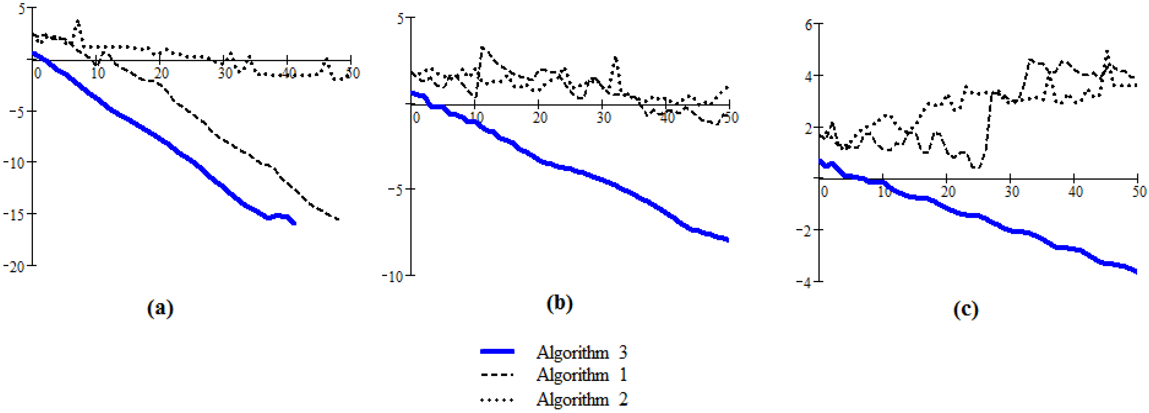
Experiment 3.
This experiment is devoted to compare Algorithm 3 with the parallel variants proposed in [
1] and [
2,
3]. Three linear systems of low dimensions (m = 5) with condition numbers equal to
were considered as test systems. Every system was set into two partitions of dimensions 3 and 2 respectively.
Figure 4.
The comparison of Algorithms 3, 1 and 2 in the care of linear systems of low dimensions (m = 5); (a) condition number = 8.598; (b) condition number=4.624; (c) condition number = 3.624.
Figure 4.
The comparison of Algorithms 3, 1 and 2 in the care of linear systems of low dimensions (m = 5); (a) condition number = 8.598; (b) condition number=4.624; (c) condition number = 3.624.
The results are presented in
Figure 4. We can conclude that the behavior of Algorithm 3 is satisfactory, as in all cases the generated sequence converges to the solution of the system and the convergence is linear. It is worthwhile to note the very good behavior of Algorithm 3 in comparison with the other two variants for cases (b) and (c): in case (b) the Algorithms 1 and 2 appear to have a very slow convergence, and in case (c) these algorithms fail to converge.


