1. Introduction
As essential terrestrial ecosystems, forests form an important part of the earth’s carbon cycle [
1,
2]. Forests not only play an indispensable role in various ecological and social services but also help maintain carbon balance and mitigate climate change, as they are considered carbon sinks [
3,
4,
5,
6,
7]. The total carbon storage of forest is equivalent to 85% of total terrestrial stocks and 75% of total terrestrial gross primary production [
8]. It is estimated that 50% of plant biomass is composed of carbon, and the estimated value of aboveground biomass (AGB) is used as a substitute for aboveground carbon [
9]. The accurate estimation of terrestrial forest biomass is conducive to better understanding the crucial role of forests in the cycle of global carbon. Therefore, the accurate estimation of AGB can reduce the uncertainty of terrestrial carbon quantification [
10,
11]. However, for many current estimates of global carbon flux and biomass distribution in forests, there is still too much uncertainty due to the coarse estimation of vegetation structures for many scientific research and policy applications [
10,
12,
13]. In regional or global mapping, the estimation of forest canopy height and AGB is directly related to the allometric growth equation. Therefore, improving the accuracy of forest canopy height estimation and enriching data sources are conducive to improving the accuracy of AGB estimation, which is an important research focus [
14].
The remote sensing system has been regarded as an indispensable practical tool because of due to its large-scale coverage and repeated observations. The combination of remote sensing satellite image data with field-measured forest inventory data can promote the production of reliable and up-to-date forest canopy height products [
15]. As an active remote sensing method, light detection and ranging (Lidar) transmits energy and records the backscattered energy from feature information of the earth’s surface. Lidar can extract three-dimensional attributes and provide vegetation metrics by converting the time taken for data to be transmitted from and returned to a sensor into distance measurements [
16]. The precise three-dimensional structure data obtained from airborne and spaceborne Lidar and measurements of forest canopy height, forest volume, and canopy cover have been successfully and widely monitored and estimated at multiple spatial scales [
16,
17,
18,
19,
20,
21].
Forest canopy height extraction based on airborne Lidar can be conducted at the single tree scale and sample plot scale. Tree heights can be extracted by the discrete point cloud and canopy height model (CHM) obtained by airborne Lidar. Pang Yong established a univariate regression model using the height of the normalized point cloud (H75) and the measured tree height and compared and analyzed the effects of high- and low-density point clouds on the retrieved stand parameters [
22]. Hirata used a watershed segmentation algorithm to identify individual trees from a CHM acquired by airborne Lidar [
23]. The recognition rate of a single tree decreases with decreasing cutting intensity from 95.3% in severe logging areas to 60% in noncutting areas. Popescu extracted tree height and crown width measurements from a CHM obtained through airborne Lidar and established linear and nonlinear regression models with measured DBH, AGB and component biomass data (leaf and root) [
16].
However, the airborne Lidar is mainly used on a small scale due to its high data acquisition costs, limited data acquisition range and use of large amounts of data, as well as being labor intensive and time consuming, and it is difficult to use for large-scale forest vertical structure information extraction and mapping [
24]. The ICESat with the Geoscience Laser Altimeter System (GLAS), as a representative spaceborne Lidar system, provides global footprint height information and is widely used in the retrieval of forest canopy heights at regional and global scales [
25,
26,
27]. Lefsky combined waveform data from the GLAS and the terrain index extracted from SRTM DEM data to correct the slope of waveform data for an area with a large slope, and improved the estimation accuracy of the regression model of the maximum forest height [
28]. The RMSE of the models for the three research areas ranged from 4.85 m to 12.66 m.
The ICESat-2 with the Advanced Topographic Laser Altimeter System (ATLAS) was launched in September 2018 as a follow-up mission to ICESat and aims to measure the structural characteristics of forests at the global scale and to complement other spaceborne Lidar missions [
29,
30], including the European Space Agency P-band radar BIOMASS [
31], the Global Ecosystem Dynamics Investigation Lidar (GEDI) [
32], and NASA-ISRO Synthetic Aperture Radar(NISAR) missions [
33]. ICESat-2 was designed to draw a global image of Earth’s third dimension with height measurements and track terrain changes, including those for sea ice, glaciers, forests, etc. (
https://icesat-2.gsfc.nasa.gov/science), as well as the first spaceborne Lidar system ICESat GLAS. Therefore, it is necessary and meaningful to explore how data obtained by ICESat-2 can be applied to estimate forest canopy height or AGB.
Montesano explored the abilities and uncertainties of ICESat-2 photon counting data in estimating coniferous forest biomass according to different biomass gradients and sampling distances along the orbit [
34]. The authors found the 50 m scale to be the optimal horizontal resolution of ICESat-2 model fitting, and the biomass level was 20 Mg/ha with the estimation error of 20% to 50%. Gwenzi evaluated the potential of ATLAS data use for canopy height extraction from savanna ecosystems [
14]. The authors found the correlation between canopy height extracted from the MATLAS simulator, which generates ATLAS-like data, and that from discrete return Lidar (DRL) to be weaker than that from Multiple Altimeter Beam Experimental Lidar (MABEL, an airborne photon counting Lidar sensor) data and predicted that the number of signal photons in spaceborne ATLAS data would be greatly reduced, causing the accuracy of canopy height estimation to decrease. Narine used simulated ICESat-2 photon counting Lidar data to generate point cloud data with the same along-orbit segmentation length as the ICESat-2 land vegetation product (ATL08), 100 m [
15]. The relationship between photon counting vegetation products and forest AGB and canopy coverage obtained by airborne Lidar was analyzed in no-noise scenes, daytime scenes and night scenes [
15]. Neuenschwander presented ATLAS data and verified the accuracy of its ground elevation [
35,
36,
37]. The RMSE value of ground elevation data obtained from the ATLAS is 0.85 m, which is lower than that of the Space Shuttle Radar topographic survey mission (SRTM).
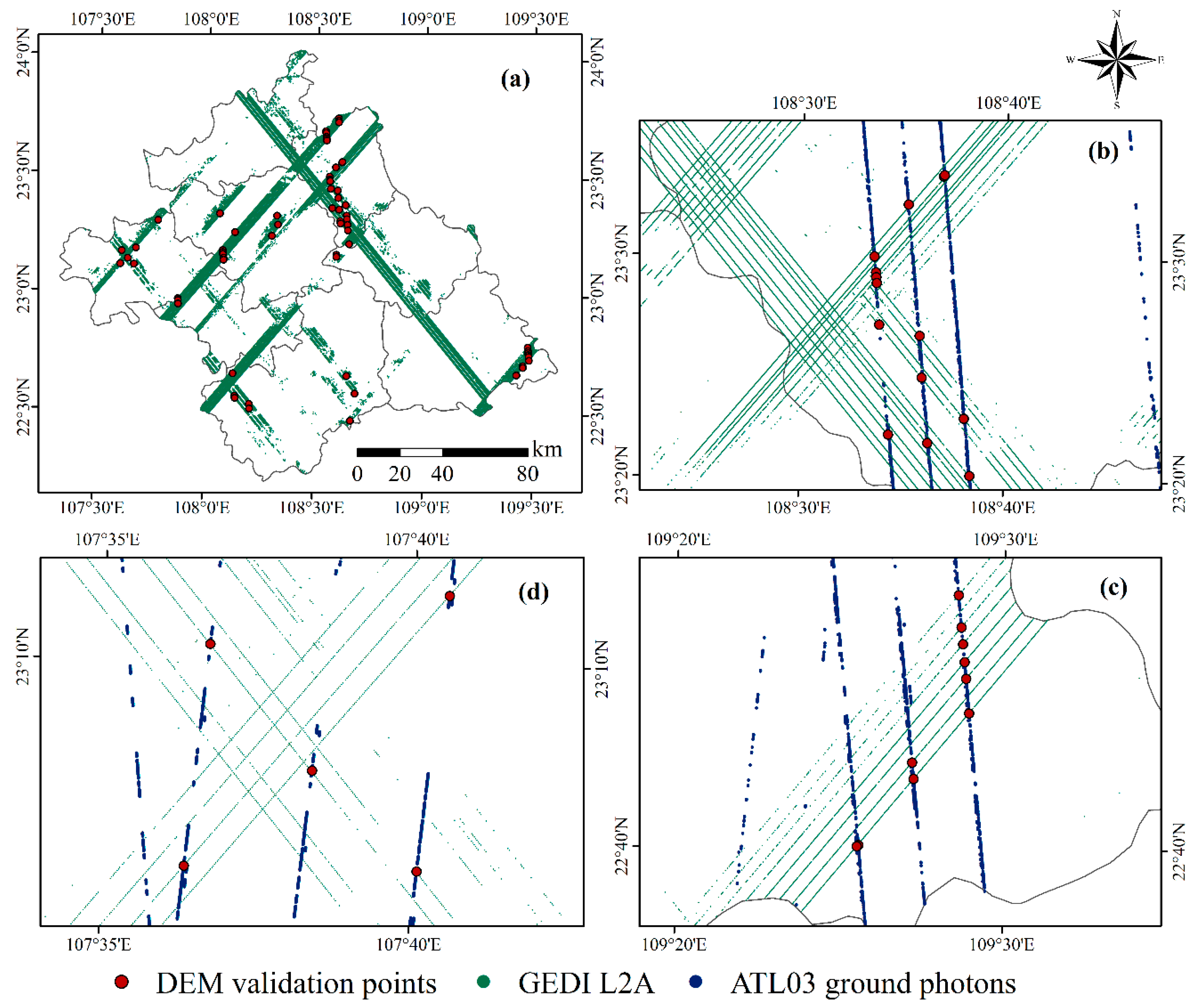
However, few studies have used ICESat-2 vegetation height products to extrapolate and map regional vegetation canopy height [
38,
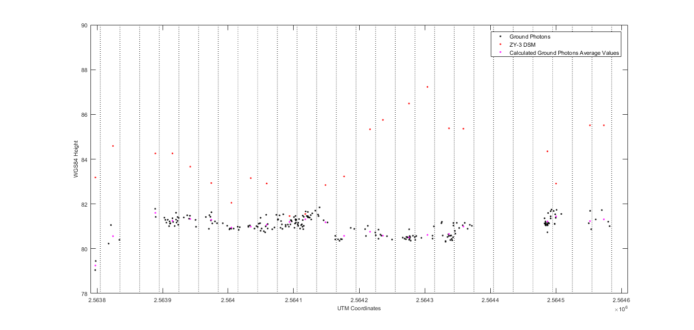
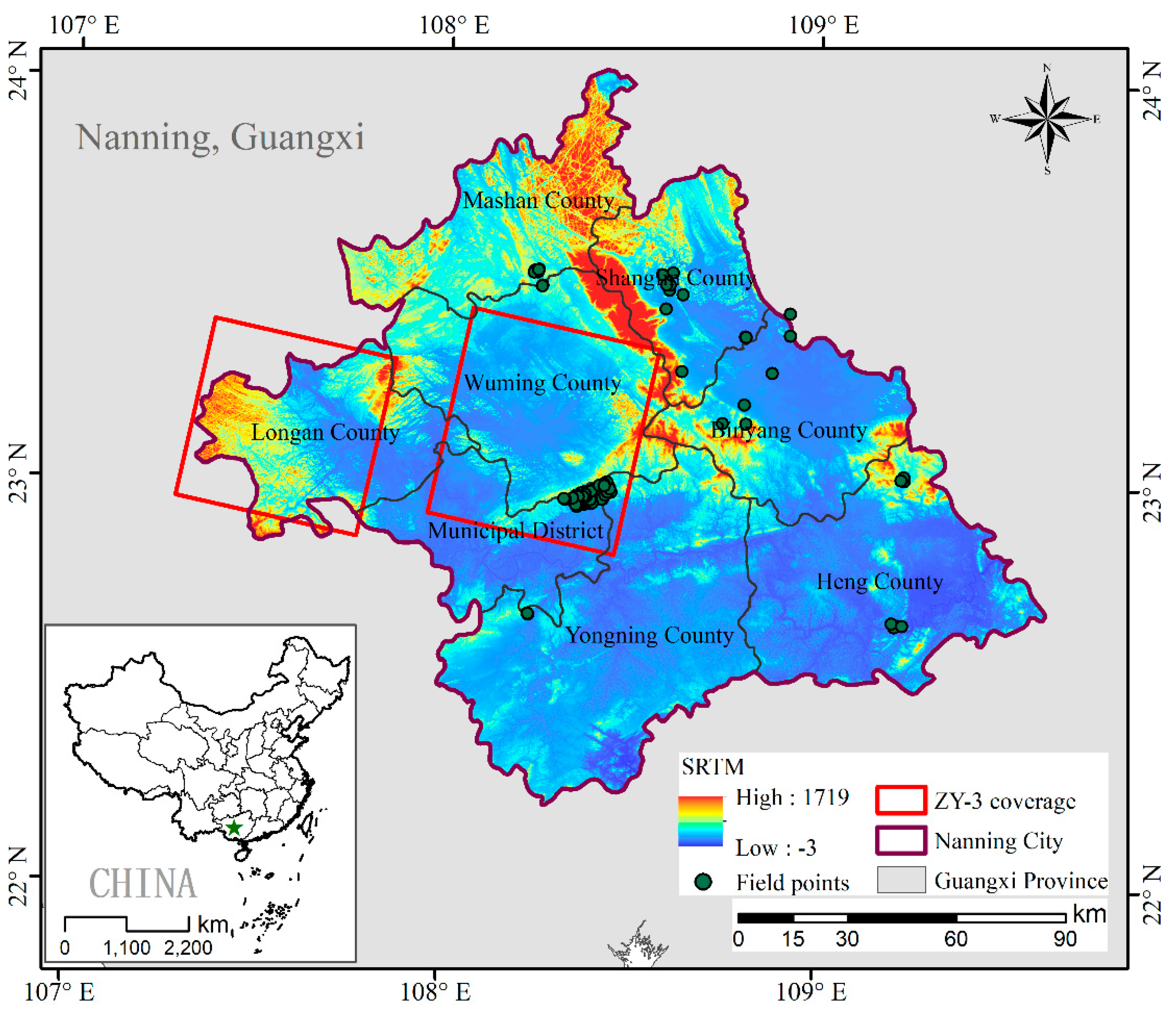
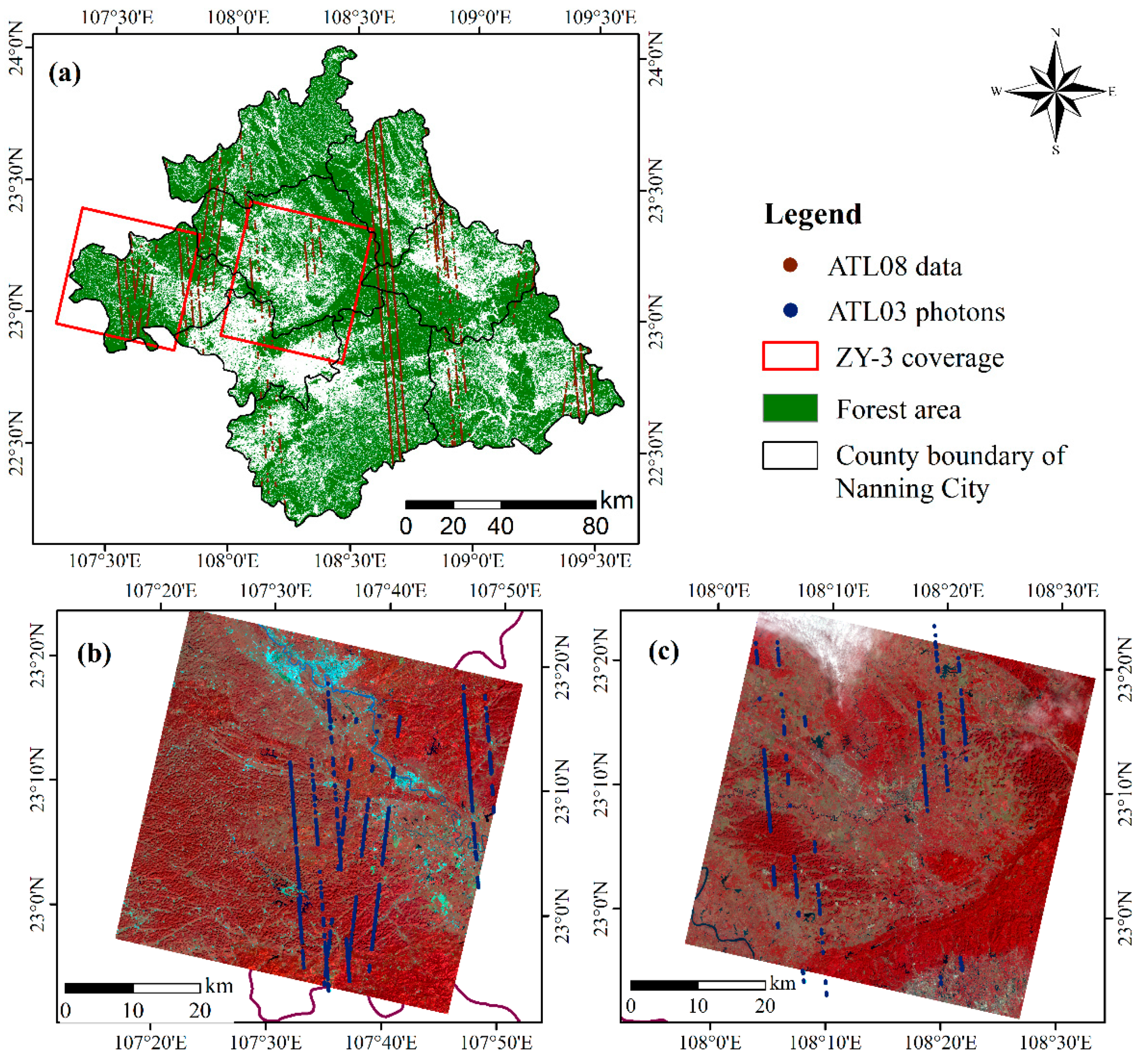
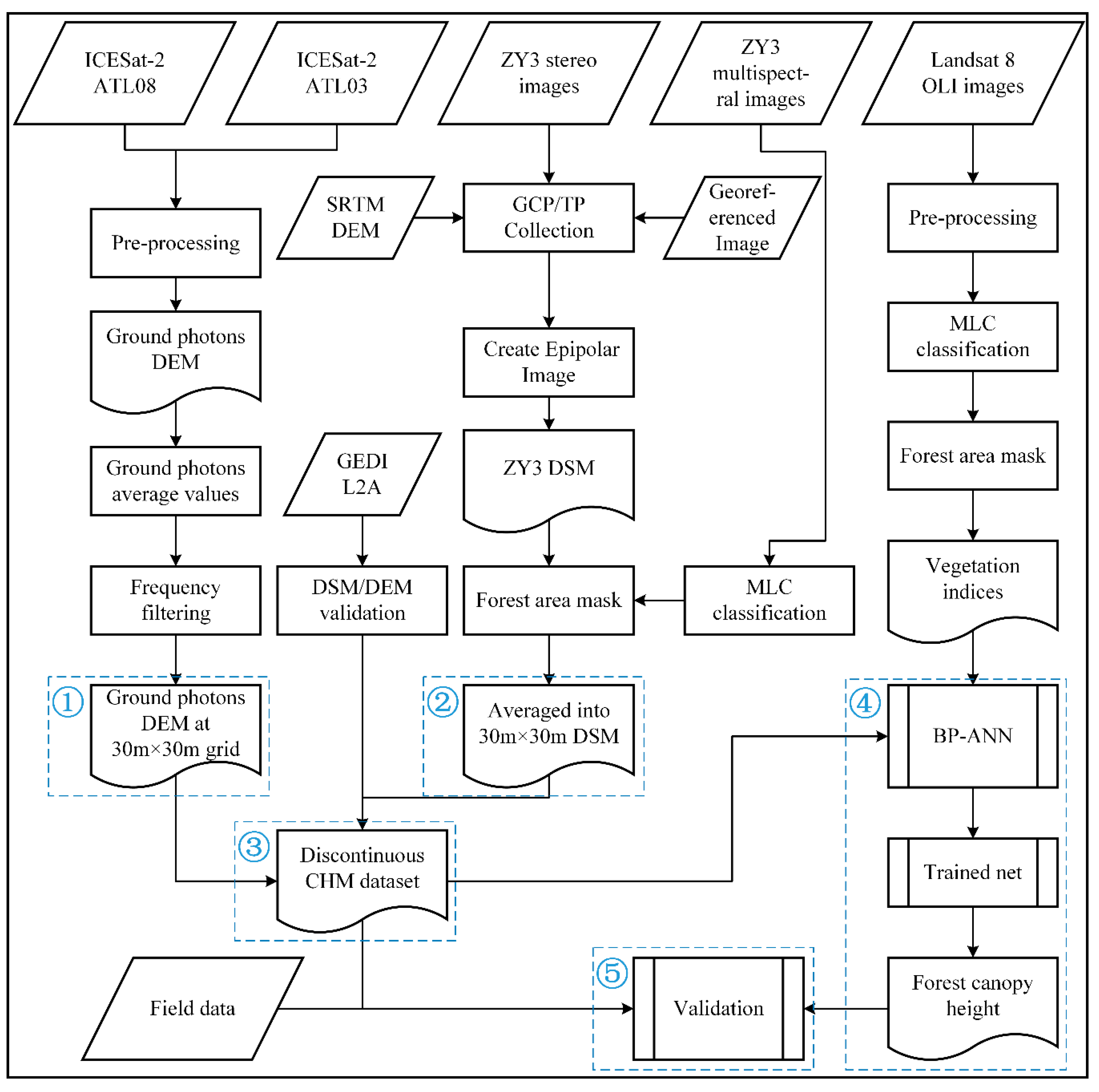
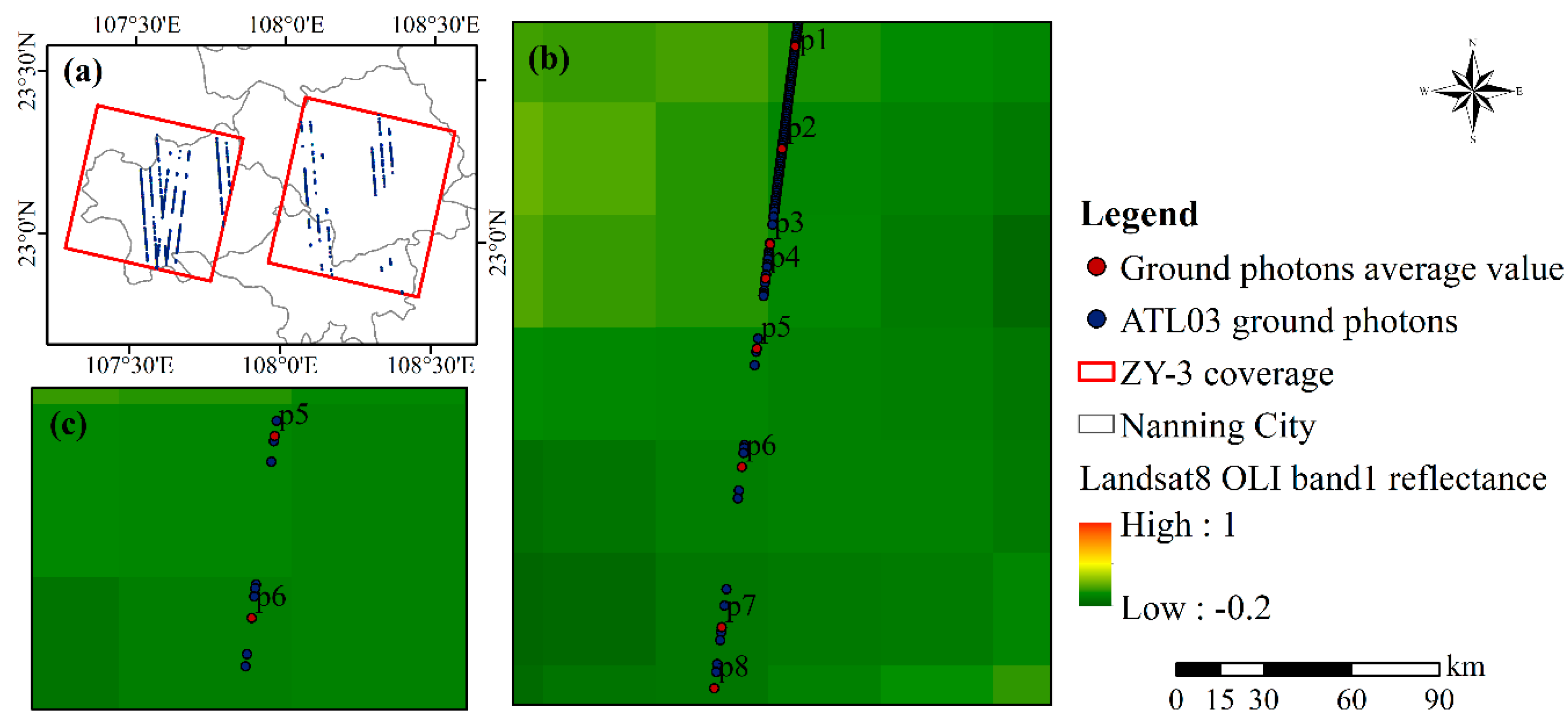
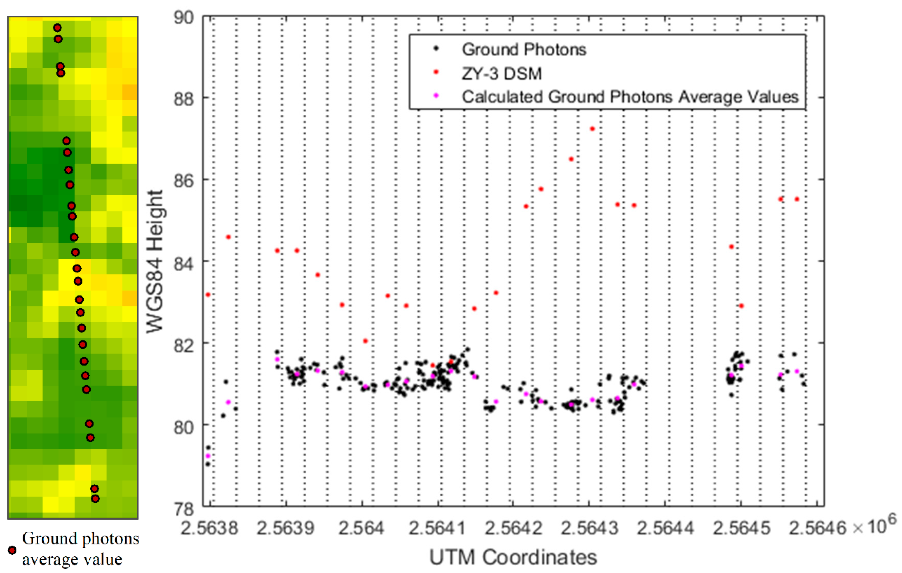
39], and most of them are based on ICESat-2 simulation data of airborne Lidar. The purpose of this paper is to explore ways to use the ATL08 and ATL03 products to map regional forest canopy heights with a 30 m resolution. There are many definitions of forest canopy height. Forest canopy height in this study refers to the mean height of trees within a given forest area. In this study, ICESat-2 ATLAS photon data and ZY-3 stereo image pair data are combined to generate a discontinuous CHM dataset. GEDI data are used to verify the accuracy of ground photon elevation and the DSM. The CHM is used to create a training sample, and the BP-ANN model is used to generate a forest canopy height map of the city of Nanning. Finally, this study analyzes resolution and how to filter effective data that emerge when ATL08 data are directly used to generate regional or global vegetation height products, which will be the focus of future research.
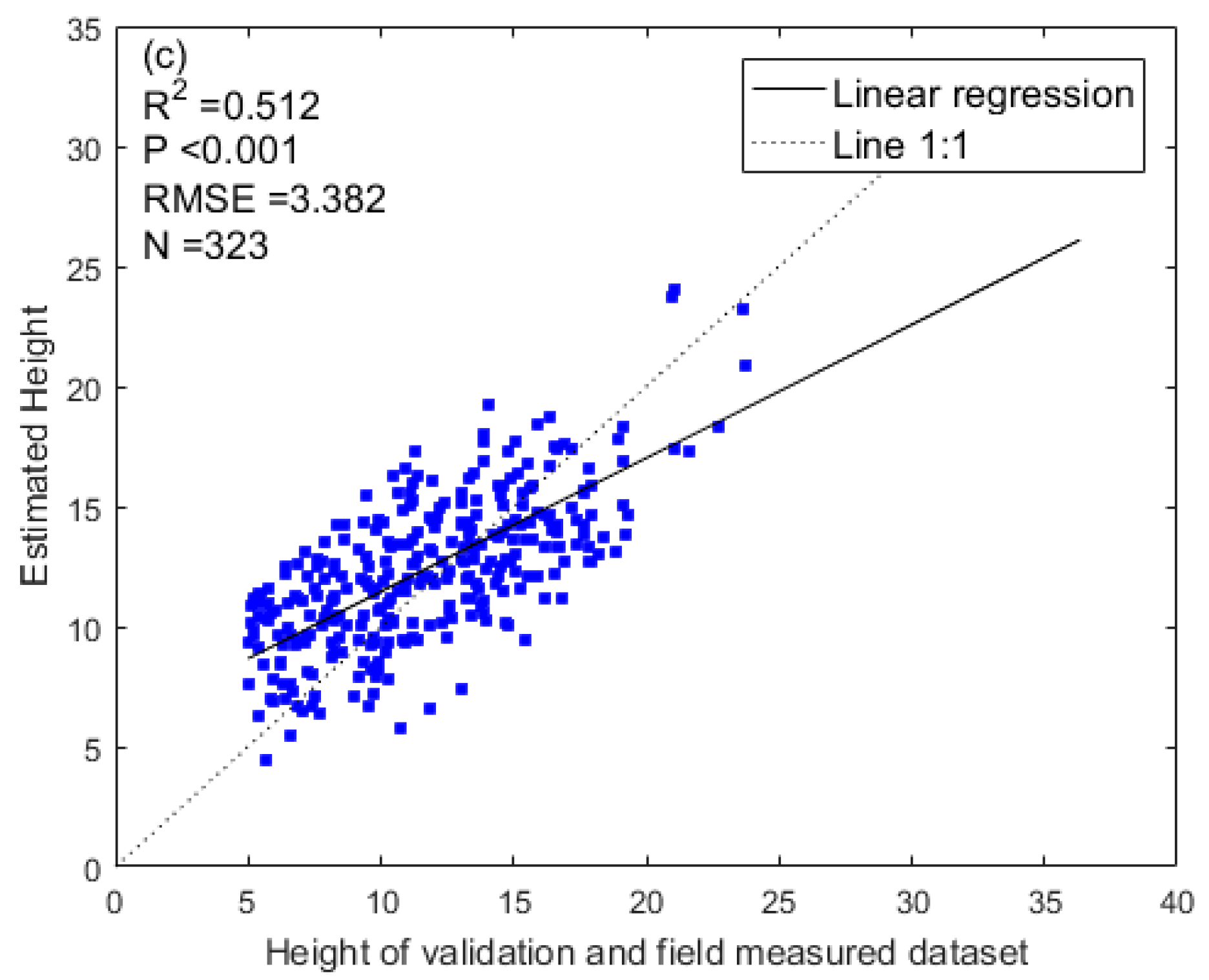
4. Discussion
4.1. Large Scale Forest Canopy Height Mapping
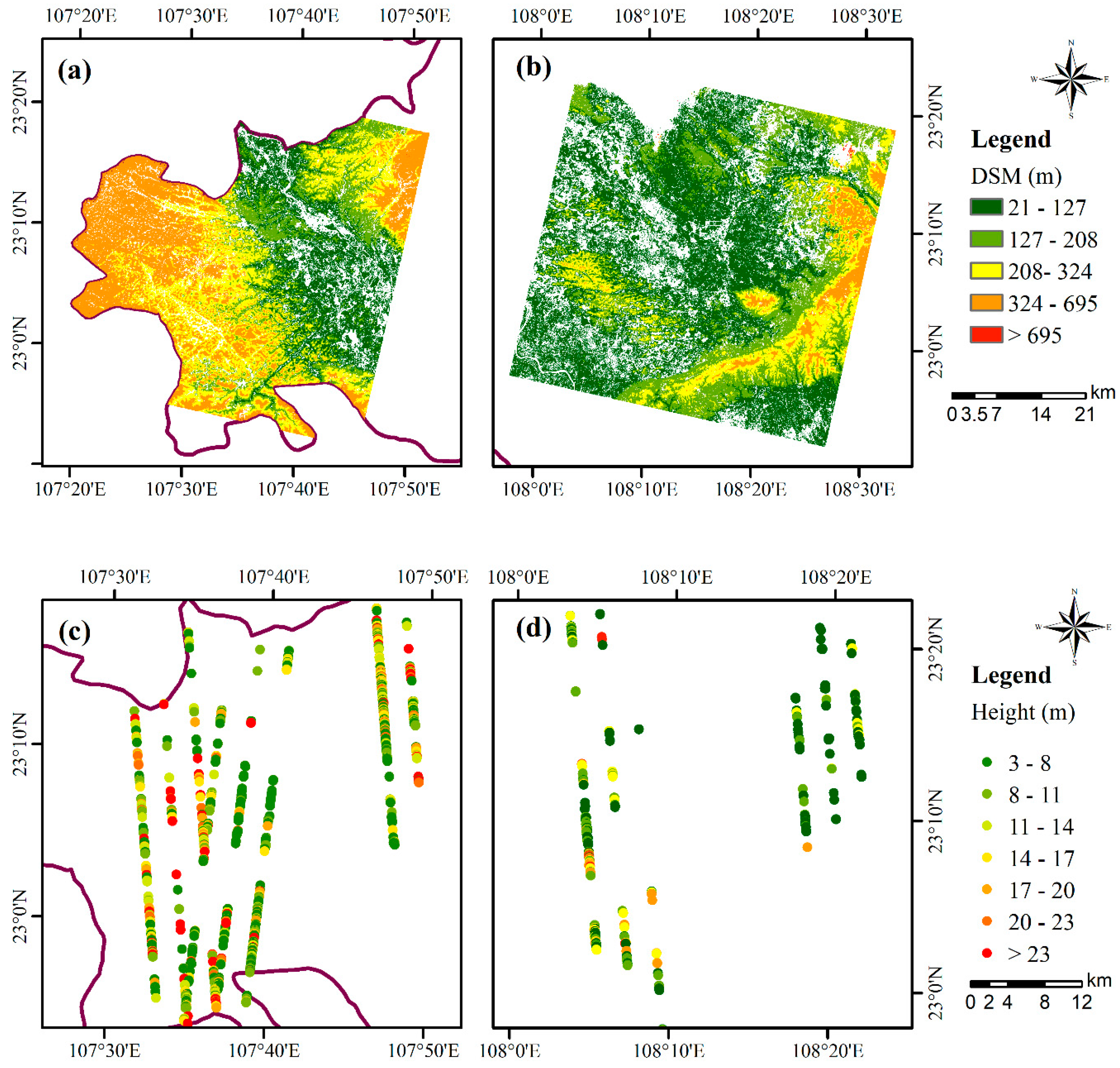
We identified a new means to estimate forest canopy height using a combination of ICESat-2 ATLAS data and stereo-photogrammetry. This method uses spaceborne Lidar ICESat-2 ATLAS data to replace airborne Lidar data and in turn obtain ground elevation information. Its low cost, unlimited data acquisition range, and global sampling range allow it to be the ability to be applied to a wider range. Given our successful application of this method to a study area in Nanning, it can be used over large scales, such as regional and global forest canopy height mapping. In addition to the stereo image pairs provided by the ZY-3 satellite, China’s first submeter high-resolution optical transmission stereo mapping satellite GF-7 can provide high-precision stereo image pair data for superimposing ICESat-2 data to estimate global forest canopy height. Although GF-2 was not designed as a photogrammetric system, some studies have made use of the different orbit data from GF-2 in repeated observation areas to realize stereo observation and extract DSM data [
65].
Additionally, other techniques such as radargrammetry can produce a DSM by using SAR images to replace the DSM derived from ZY-3 in this study [
44,
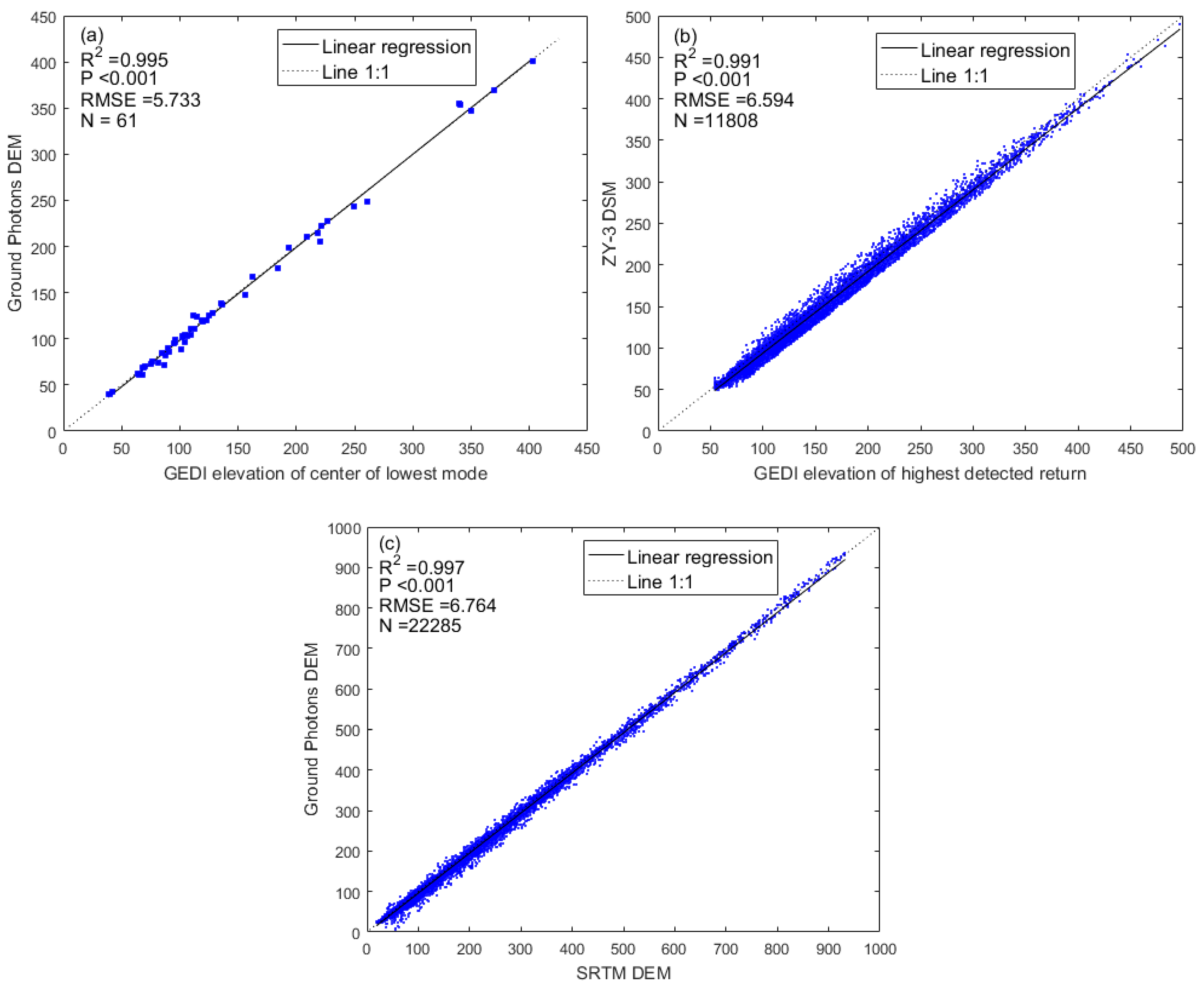
45]. In addition to ICESat-2, the GEDI can provide surface elevation information as a DEM [
32,
57,
58].
In addition, to obtain mapping results with the same resolution as those of Landsat, 30 m × 30 m grid is used to process ground photons. If we want to obtain a lower resolution result, such as those of the Moderate Resolution Imaging Spectroradiometer (MODIS), this is feasible, but for higher resolution mapping, we should consider enough ground photons to increase the accuracy and reliability of the DEM. Further analysis and research are needed.
4.2. How to Filter Effective ATL08 Data
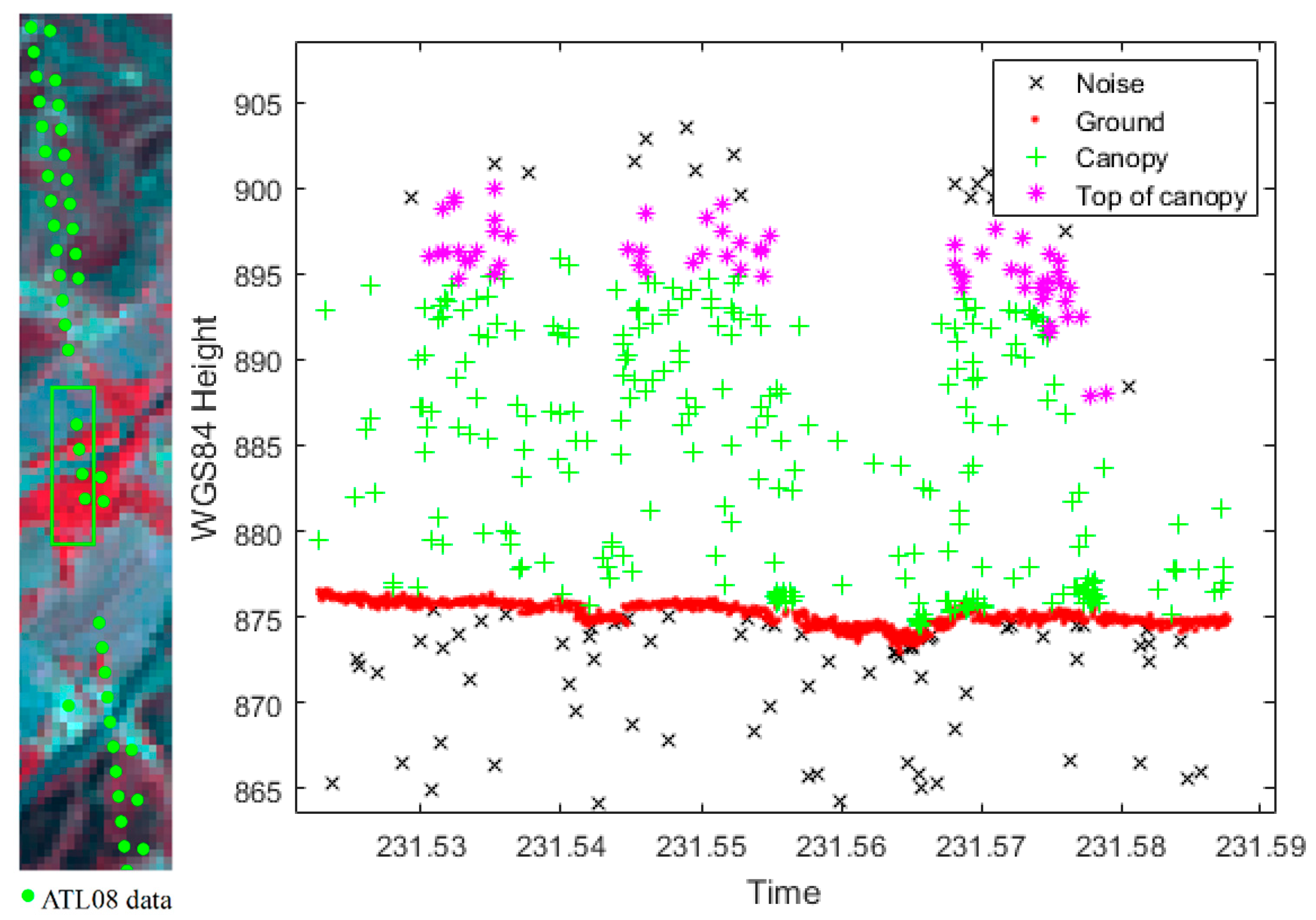
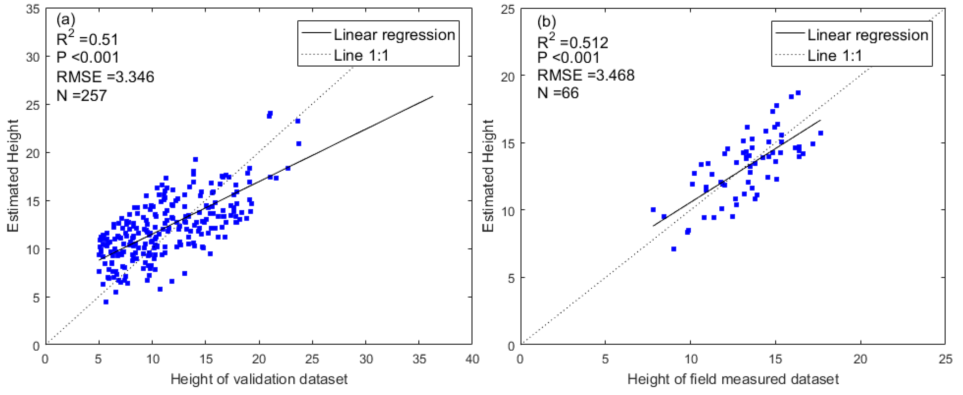
The canopy height values provided by ATL08 data can be used as samples to directly generate a wall-to-wall forest canopy height map. Since the resolution of ATL08 data is 100 m, ATL08 data are not suitable for vegetation mapping at a 30 m resolution as with Landsat data, and should be used to map at resolutions of greater than 100 m to eliminate errors caused by position deviations. The selection of effective ATL08 data is a key problem. These two fitting lines are highly dependent on the accuracy of photon classification, creating inevitable errors in the canopy height values of ATL08.
Our numerical analysis shows that, for ATL08 data of the study area, 6% of canopy height values are greater than 50 m, which can be considered invalid values. These invalid values may originate from the low precision surface and vegetation surface curves fitted by sparse signal photons, or even attribute values obtained by interpolation. For the remaining 94% of the data, even if we use the rest of the ATL08 data fields (such as clouds, snow, and urban areas) to exclude the influence of land surface types and clouds, the reliability of canopy height data is affected by many other factors. For instance, (1) irregular topography increases photon classification errors, and (2) when the photon signal of a surface or vegetation is weak and the number of point clouds is small, the fitting error of the surface curve will increase.
Many uncertain factors make it difficult to automatically filter effective data when data are used in regional mapping.
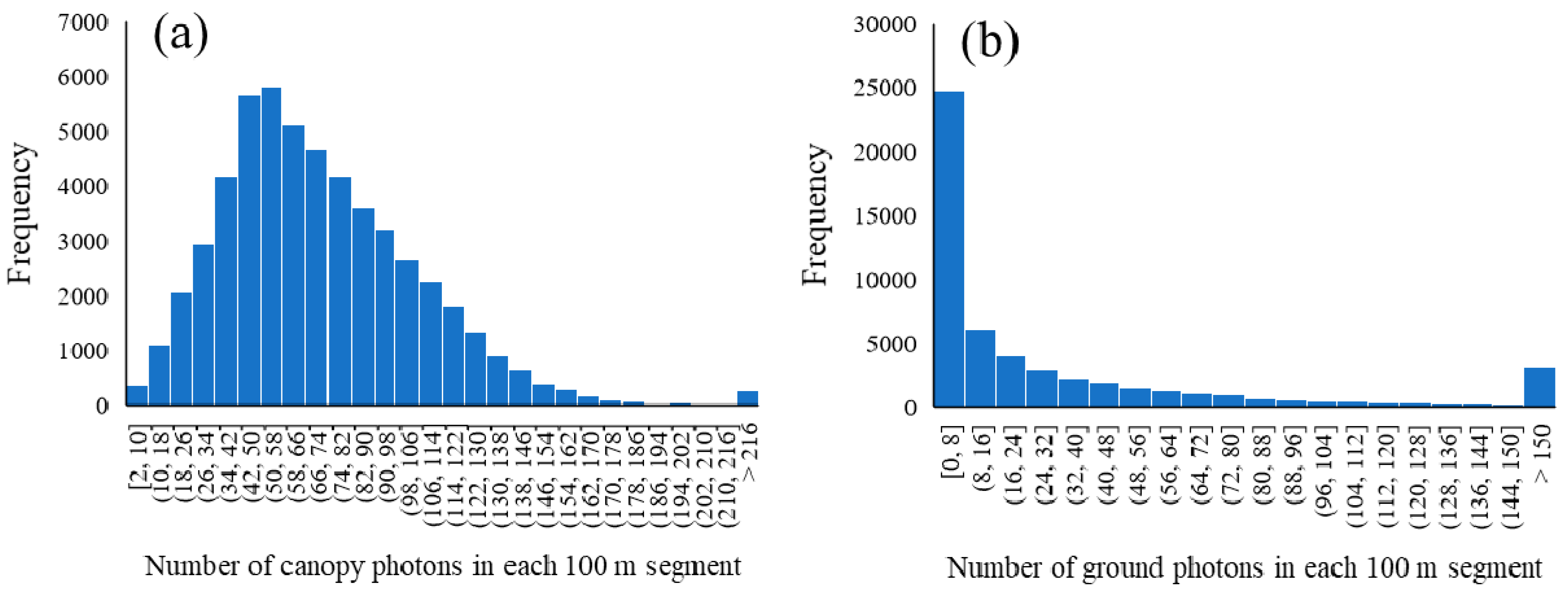
Figure 12 shows a frequency statistics histogram of canopy and ground photons. We suggest that canopy and ground photon numbers be used as a basis for screening effective ATL08 data, as the stronger the photon signal, the smaller the error becomes. However, determining the photon number threshold with universal or adaptive rules is an issue worthy of future research.

 ,
, 


