Reconstruction of Spatiotemporally Continuous MODIS-Band Reflectance in East and South Asia from 2012 to 2015

Abstract

To reconstruct Moderate Resolution Imaging Spectroradiometer (MODIS) band reflectance with optimal spatiotemporal continuity, three bidirectional reflectance distribution function (BRDF) models—the Ross-Thick-Li-Sparse Reciprocal (RTLSR) model, Gao model, and adjusted BF model—were used to retrieve MODIS-band reflectance for cloudy MODIS pixels according to different inversion conditions with a proposed filling algorithm. Then, a spatiotemporally continuous MODIS-band reflectance dataset for most of Asia with more than 98% spatiotemporal coverage was reconstructed from 2012 to 2015. The validation highlighted an evident improvement in filling cloudy MODIS observations; a reasonable spatial distribution, such as in South Asia and Southeast Asia; and acceptable precision for the filled MODIS pixels, with the root mean square error percentage (RMSE%) at 9.7–9.8% and 12–16% for the Gao and adjusted BF models, respectively. In the course of reconstructing the spatiotemporal continuous MODIS-band reflectance, the differences among the three models were discussed further. For a 16-day period with a stable and unchanged land surface, the RTLSR model, as a basic model, accurately derived land surface reflectance (no more than 10% RMSE% for MCD43C1 V006 band 1) and outperformed the other two models. When the inversion period is sufficiently long (e.g., 108 days, 188 days, 268 days, or a full year), the Gao/adjusted BF model provides better precision than the RTLSR model by considering the normalized difference vegetation index (NDVI) and soil moisture/NDVI as intermediate variables used to adjust the BRDF parameters in real time. The Gao model is optimal when the inversion period is sufficiently long. Based on combining the RTLSR model and Gao/adjusted BF model, we proposed a filling algorithm to derive a dataset of MODIS-band reflectance with optimal spatiotemporal continuity.

1. Introduction

Since 1967, when the planning and development of the first Landsat satellite commenced, remote sensing science has developed, and many remotely sensed observations have been archived. In addition to the Landsat satellites launched in 1972—including the Multispectral Scanner System (MSS), Thematic Mapper (TM), Enhanced Thematic Mapper plus (ETM+) and Operational Land Imager (OLI) [1,2,3]—the Moderate Resolution Imaging Spectroradiometer (MODIS) has obtained time series of remotely sensed observations for nearly 20 years [4,5]. Moreover, many remotely sensed products for the atmosphere, biosphere, and hydrosphere have been derived, and net radiation, albedo, normalized difference vegetation index (NDVI), soil moisture, and evapotranspiration data have been obtained [6,7,8,9,10]. Based on the aforementioned progress in remote sensing science, remotely sensed products have been adopted to answer scientific problems in many fields, such as in land and surface water mapping for evaluating climate change [11,12]. However, the spatiotemporal discontinuity of remotely sensed observations caused by clouds has impeded the application of various remotely sensed products in the scientific community. For example, MODIS NDVI products are produced from daily remotely sensed observations every 16 days considering cloud cover and the MODIS solar-viewing geometry [5]. The discontinuities in soil moisture derived from microwave remotely sensed observations are partly caused by clouds, although microwave observations have all-weather features. In addition, land cover classification and lake identification based on Landsat sensors, MODIS and other satellite observations are derived on 1-year and several-year cycles [13,14,15,16]; obviously, clouds are an important factor in decreasing the temporal resolution of classification products. The spatiotemporal discontinuity of remotely sensed products has become a bottleneck in their use in various scientific fields.

In the remote sensing community, observations and technology are improving, thus providing an opportunity to improve the spatiotemporal continuity of remotely sensed products. Notably, researchers have used Harmonic ANalysis of Time Series (HANTS) to interpolate daily NDVI based on the MODIS NDVI product [5,8]. A general regression neural network (GRNN) was introduced to fill the gaps in daily soil moisture data sets by considering the relations among several land surface parameters (temperature, NDVI, albedo, and others) [17]. A method that merges Landsat and Sentinel observations improved the temporal resolution of NDVI data for monitoring crops [18]. In addition to the aforementioned research that focused on eliminating the negative effect of clouds on remote sensing results, some image processing methods—such as time-based methods, space-based methods, spectral-based methods, and hybrid methods—may be effective in eliminating cloud issues [19].

MODIS, as the most successful satellite, produces plenty of products, and the observation period is nearly 20 years [16,20,21,22]; the subsequent mission was the Visible Infrared Imaging Radiometer Suite (VIIRS) [23]. However, the MODIS spatiotemporal discontinuity mainly caused by clouds and other factors may hinder the broad use of MODIS data, and eliminating the negative effects of clouds is important for the development of remote sensing methods. Luckily, MODIS research teams proposed an algorithm for deriving the bidirectional reflectance distribution function (BRDF) and albedo [7,22], and it can be used to eliminate the negative effects of clouds by filling cloudy MODIS observations [24]. For a consistently cloudy area (e.g., Southeast Tibet, the Yunnan–Guizhou Plateau, and the southern part of the Yangtze River basin in the growing season), however, the MODIS official algorithm may be invalid due to insufficient data set derivation in a short inversion period with stable land cover (e.g., 16 days); thus, a back-up algorithm is adopted to fill data gaps [22,25]. Obviously, the filled values may be inaccurate due to the lack of a theoretical basis; in fact, such values may produce abnormal results. The reconstruction of MODIS-band reflectance on consecutive cloudy days with sufficient precision could greatly improve spatiotemporal continuity and help promote the use of remotely sensed data sets in different scientific communities.

Based on the physical mechanisms of the BRDF model, Vermote et al. suggested an algorithm for quantifying the variation in the BRDF shape based on the periodized NDVI [26]. Although previous research on the anisotropic flat index (AFX) demonstrated that the NDVI is not always a reliable index of the reflectance anisotropy in different methods [27,28,29], Franch introduced the NDVI as a normalized intermediate parameter of a kernel-driven model to derive albedo at different spatiotemporal resolutions [30,31,32,33]. Other researchers proposed an improved kernel-driven model by coupling soil moisture and the NDVI with the Ross-Thick-Li-Sparse Reciprocal (RTLSR) model, thus creating the so-called ‘Gao model’ [34]. The ‘Gao model’ introduces the NDVI and soil moisture into the RTLSR model and can derive the dynamic parameters of the BRDF model to encompass the anisotropic reflectance of the changing land surface, thereby largely overcoming the limitations of the RTLSR model. We can derive the Gao model by creating a sufficient input dataset for a sufficiently long inversion period, for example, several months or a full year, thus promoting the valid derivation of the BRDF model. Previous research indicated that the improved RTLSR model has acceptable precision (root mean square error percentage (RMSE%) of 7%) for a more than 70-day inversion period globally [34]. In addition, a so-called ‘adjusted BF model’ based on Franch’s research introduced the NDVI as a parameter dynamically used to adjust the land surface BRDF. Based on the aforementioned research, we believe that the above BRDF models expanded from the RTLSR model can be used to mitigate the invalid retrieval problem of the MODIS official algorithm for BRDF/albedo [7].

In addition to the well-matched BRDF models, we need spatiotemporally continuous soil moisture and NDVI data to derive cloudy MODIS-band reflectance. For soil moisture, the released products have coarse spatial resolutions (e.g., Soil Moisture Ocean Salinity (SMOS) and Soil Moisture Active Passive (SMAP) products) or low temporal resolutions (e.g., fusing SMAP and Sentinel). Additionally, the algorithm limits for soil moisture products often lead to invalid retrievals [35]. Notably, preprocessing is necessary for spatiotemporally continuous soil moisture, and the GRNN method was proposed; specifically, the relationships between soil moisture and several other land surface parameters were obtained (albedo, the NDVI, temperature, and others) to fill invalid soil moisture pixels [17]. Then, the HANTS method was applied to interpolate daily NDVI values based on every 16-day MODIS NDVI product [8].

After the aforementioned introductions and preparations, we use the Gao model and adjusted BF model to derive cloudy MODIS-band reflectance due to invalid retrieval based on the official MODIS product (MCD43C1 V006); specifically, postprocessing is performed for daily soil moisture and MODIS NDVI data. Then, a spatiotemporally continuous MODIS-band reflectance data set is reconstructed for East and South Asia from 2012 to 2015. In the performing course, we also perform retrieval based on the BRDF models (e.g., RTLSR model, Gao model, and adjusted BF model) for the other two objectives: (1) evaluating the precision and efficiency of the BRDF models and (2) determining the priority of the BRDF models in filling cloudy MODIS pixels in the proposed algorithm. Section 2 introduces the theoretical basis of the selected BRDF model, details the process of constructing the proposed BRDF model, and presents the theoretical retrieval of spatiotemporally continuous MODIS-band reflectance. Section 3 details the experimental areas, introduces the experimental dataset and describes the preprocessing of soil moisture and NDVI data. Section 4 describes the experiments in East and South Asia, and the results are used to evaluate the accuracy of the BRDF model and spatiotemporal pattern of the assessed models (e.g., the Gao model and adjusted BF model) to determine which one is superior in the derivation of cloudy MODIS-band reflectance. Section 5 describes the improvement in the reconstructed MODIS-band reflectance datasets. Finally, Section 6 summarizes the results, discusses the limitations of the research and proposes ways to enhance the model.

2. Model and Method

2.1. BRDF Model

As the basic BRDF model in our research, the RTLSR model is the primary model used in the algorithm for MODIS BRDF/albedo products and describes the BRDF as a linear superposition of a set of kernels that reflect basic BRDF shapes; the corresponding relation has the following form [36,37,38,39,40]

$$BRDF\left({\theta }_i,{\theta }_v,{\varphi }_v,{\varphi }_i\right)=f_{iso}+f_{vol}{k}_{RT}\left({\theta }_i,{\theta }_v,{\varphi }_v,{\varphi }_i\right)+f_{geo}{k}_{LSR}\left({\theta }_i,{\theta }_v,{\varphi }_v,{\varphi }_i\right)$$

(1)

where f_vol, f_geo, and f_iso represent the coefficients of the Ross-Thick scattering kernel k_RT, Li-Sparse Reciprocal geometrical optical kernel k_LSR and isotropy 1, respectively, and θ_i, θ_v, Φ_v, and Φ_i represent the solar zenith, viewing zenith, viewing azimuth, and solar azimuth of the solar-viewing geometry, respectively.

In Vermote’s research, the NDVI was introduced as an intermediate variable in the kernel-driven model. In addition, the normalized BRDF model parameters vary linearly with the NDVI over the full year and with the albedo with an acceptable accuracy [26]. Franch et al. verified the different empirical relationships between spectral reflectance and the NDVI and showed that the BRDF can be constructed based on multiple land surface parameters. The BRDF model from Vermote’s research and Franch’s research was constructed based on the hypothesis that the normalized model parameters vary linearly with the NDVI over the full year [32]. Based on Franch’s research, we slightly adjusted this hypothesis for efficiency. The adjusted hypothesis is that the model parameters vary linearly with the NDVI N_DVI over a long period (e.g., several months or a full year), and the adjusted BF model was constructed based on the adjusted hypothesis (Equation (2))

$$BRDF\left({\theta }_i,{\theta }_v,{\varphi }_v,{\varphi }_i,N_{DVI}\right)=f_{iso}+f_{vol\_n}{k}_{RossThick}\left({\theta }_i,{\theta }_v,{\varphi }_v,{\varphi }_i\right)+f_{geo\_n}{k}_{LSR}\left({\theta }_i,{\theta }_v,{\varphi }_v,{\varphi }_i\right)$$

(2)

where

$$\begin{gathered} f_{vol\_n}=a_0+a_1{N}_{DVI} \\ {f}_{geo\_n}=a_2+a_3{N}_{DVI} \end{gathered}$$

In previous research, the above hypothesis was adjusted further; notably, the BRDF model parameters f_vol and f_geo were assumed to vary linearly with the NDVI N_DVI and soil moisture S_m over long periods (e.g., several months or a full year). Then, the Gao model was constructed (Equation (3)) [34]

$$BRDF\left({\theta }_i,{\theta }_v,{\varphi }_v,{\varphi }_i,S_m,N_{DVI}\right)=f_{iso}+f_{vol\_ns}{k}_{RossThick}\left({\theta }_i,{\theta }_v,{\varphi }_v,{\varphi }_i\right)+f_{geo\_ns}{k}_{LSR}\left({\theta }_i,{\theta }_v,{\varphi }_v,{\varphi }_i\right)$$

(3)

where

$$\begin{gathered} f_{vol\_ns}=a_0{S}_m+a_1{N}_{DVI} \\ {f}_{geo\_ns}=a_2{S}_m+a_3{N}_{DVI} \end{gathered}$$

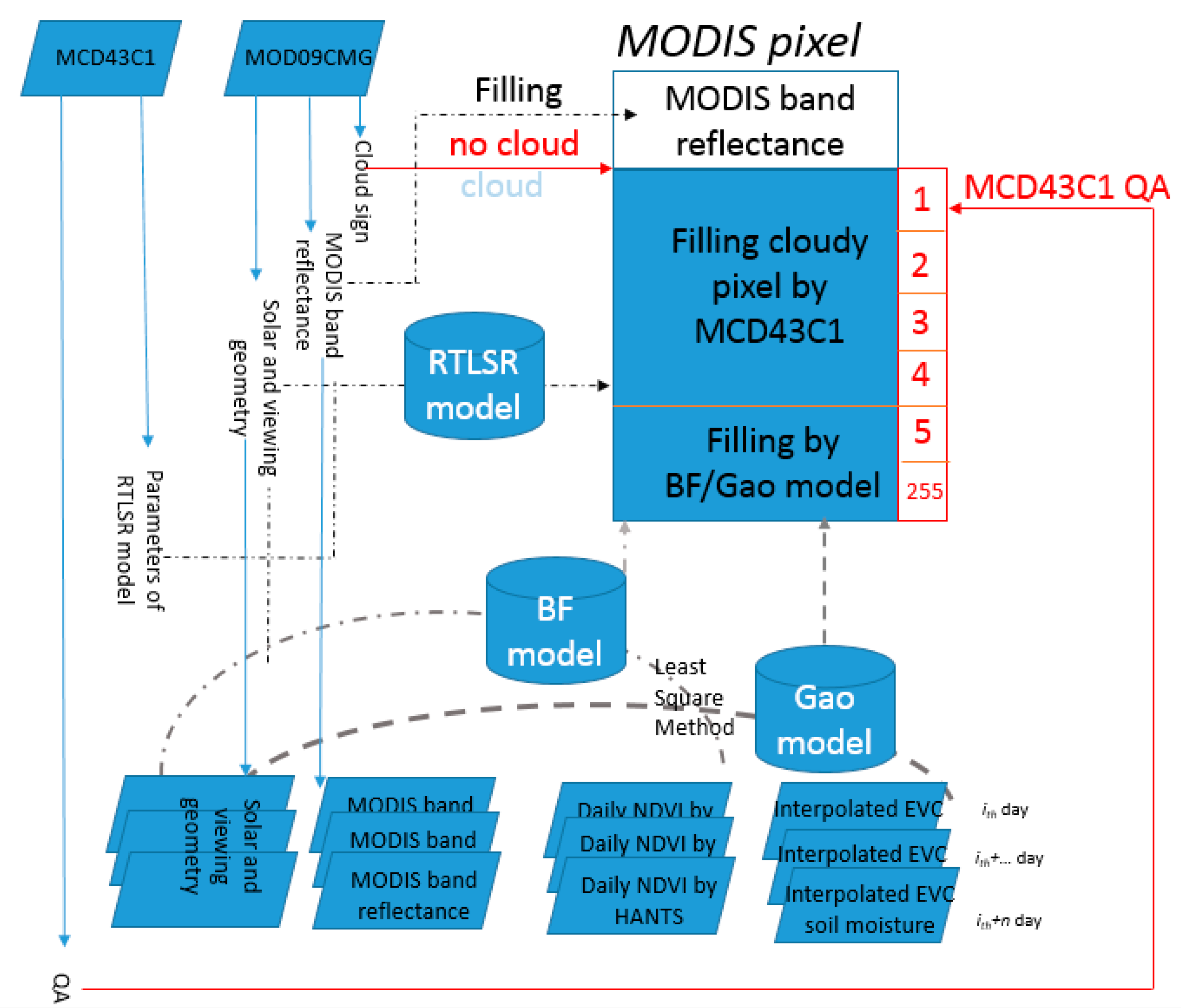
2.2. Algorithm for the Reconstruction of MODIS-Band Reflectance

The key to reconstructing spatiotemporally continuous MODIS-band reflectance is proposing an algorithm that can use the advantages of BRDF models. First, we utilize cloud signs from Terra MODIS land surface reflectance with a 0.05° Climate Metrology Grid (CMG) (MOD09CMG V006) to classify MODIS pixels into cloudy pixels and no-cloud pixels. For no-cloud pixels, spectral reflectance values from MODIS-band observations are adopted; for cloudy pixels, we choose different BRDF models to derive the MODIS-band reflectance of the land surface.

The differences among the three models based on the performance, limits, and behavior were assessed. The RTLSR model has the optimal behavior for short inversion periods (e.g., 16 days), and as the inversion period expands (e.g., two months), the Gao model and adjusted BF model become more accurate (the Gao model is optimal, and the adjusted BF model ranks second). Therefore, the RTLSR model parameter from MCD43C1 V006 is the first choice for filling MODIS cloudy pixels, and the quality assessment (QA) based on MCD43C1 V006 yield classes labeled 1, 2, 3, and 4. When the QA of MCD43C1 V006 is between 5 and 255, the Gao model is used first, and the adjusted BF model is applied second [22]. In previous research, the Gao model displayed better precision than the adjusted BF model for long inversion periods [34], and this finding is similar to the conclusion of the retrieval performed based on the RTLSR, Gao, and adjusted BF models for inversion periods from 108 days to 268 days.

Toward the reconstruction of spatiotemporal continuous MODIS band reflectance, the proposed filling algorithm was performed after the preprocessing of input datasets, which included the following steps:

(1) The no-cloud MODIS observations (e.g., MOD09CMG V006) are used for filling the no-cloud MODIS pixels, and the no-cloud/cloudy MODIS pixels are identified by the cloud sign from MOD09CMG V006.

(2) For the cloudy MODIS pixels, MCD43C1 V006 product is preferred for filling MODIS cloudy pixels while QA of MCD43C1 V006 being labeled 1, 2, 3, and 4.

(3) For the cloudy MODIS pixels with MCD43C1 V006 QA being labeled 5 and 255, we make use of least square method to derive a couple of parameters of Gao model based on the time series of no-cloud MODIS band 1–7 reflectance and the corresponding input parameters (e.g., MODIS solar - viewing geometry, Daily NDVI, and soil moisture) within the different inversion period: 108-day, 188-day, and 268-day; and the cloudy MODIS pixels can be filled by the derived Gao model’s parameter and the corresponding input parameters. For filling the cloudy MODIS pixels, the retrieval based on the 108-day inversion period is optimal, that based on the 188-day inversion period comes second, and that of the 268-day inversion period is third.

(4) After the aforementioned three steps, there are still a few cloudy MODIS pixels being not filled; and the adjusted BF model can be used for filling process, which is same as the Step 3.

A full flowchart is shown in Figure 1, which includes the preprocessing of input datasets, identification of cloudy pixels, and implementation of the proposed filling algorithm based on the different QAs (see Figure 1).

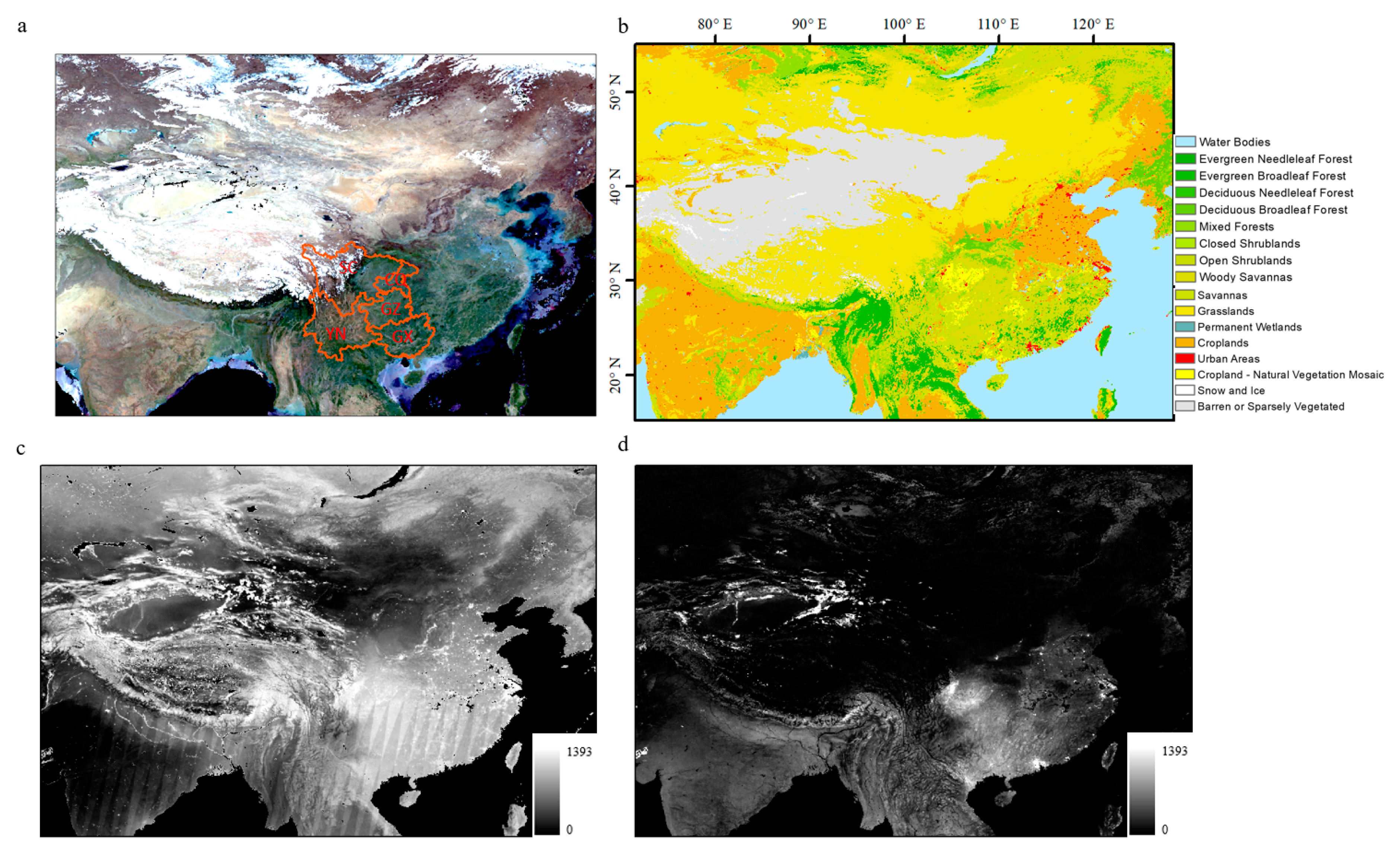
3. Experimental Area and Data

In the proposed research, two key steps are necessary: constructing the well-matched BRDF models for different cloudy MODIS pixels and developing a time series of input datasets (e.g., soil moisture, NDVI, MODIS-band reflectance, and MODIS solar-viewing geometry). For the well-matched BRDF models, the Gao model is developed based on the time series of soil moisture, the NDVI, MODIS-band reflectance, and MODIS solar-viewing geometry and is regarded as the first model used to fill cloudy MODIS pixels with QA 5 to 255 values (QA 5 indicates that filling is needed, and QA 255 is no filling). The precision of the adjusted BF model was found to be worse than that of the Gao model in this research and in previous work [34], but the derivation of the adjusted BF model needs only the NDVI, MODIS-band reflectance, and MODIS solar-viewing geometry, resulting in a lower inversion threshold than that of the Gao model; therefore, the adjusted BF model is able to overcome the invalid retrieval issue of the Gao model caused by the lack of soil moisture. Obviously, applying such an algorithm that fills cloudy MODIS pixels with QA 5 to 255 values is more scientific and credible than using a filling value [22].

In addition to the well-matched BRDF model in the proposed filling algorithm for cloudy MODIS pixels, sufficient input datasets with good spatiotemporal continuity are important for the derivation of spatiotemporally continuous MODIS-band reflectance. Nevertheless, the available soil moisture and NDVI data are often poor. The mainstream soil moisture products (SMOS, SMAP, and AMSR2) commonly have low precision, low spatial resolutions, and low spatiotemporal continuity [35,41]. For example, the SMAP L3 Radar/Radiometer Global Daily 9-km EASE-Grid Soil Moisture product, which is largely considered to have the best accuracy among soil moisture products, has poor spatiotemporal continuity. Therefore, our team constructed a daily soil moisture data set from 2012 to 2015 for East and South Asia (UL: 70°E, 55°N, DR: 130°E, 15°N). Data from the Climate Change Initiative (CCI) project of the European Space Agency (ESA) Program on the Global Monitoring of Essential Climate Variables (ECV), including soil moisture, land surface temperature, NDVI, and albedo data at 0.05° CMG, were applied based on a machine learning method called GRNN [17,42]. Another key input parameter, daily NDVI, was reconstructed based on MOD/MYD09GA V006 by our team with HANTS, as adopted in previous research [8]. All the input datasets are shown in

Table 1. Experimental data.

Data	Data Set Name	Spatiotemporal Coverage	Resolution
Soil moisture	EVC soil moisture Interpolated by GRNN	UL: 70°E, 55°N, DR: 130°E, 15°N; and from 2012 to 2015	0.05° and daily
NDVI	MOD09CMG V006 Interpolated by HANTS	UL: 70°E, 55°N, DR: 130°E, 15°N; and from 2012 to 2015	0.05° and daily
Spectral reflectance	MOD09 CMG V006	UL: 70°E, 55°N, DR: 130°E, 15°N; and from 2012 to 2015	0.05° and daily
BRDF parameters	MCD43C1 V006	UL: 70°E, 55°N, DR: 130°E, 15°N; and from 2012 to 2015	0.05° and daily
Land cover	MCD12Q1 V006	UL: 70°E, 55°N, DR: 130°E, 15°N; and from 2012 to 2015	0.05° and yearly

.

Due to the limited spatiotemporal range of soil moisture adopted in our research, we selected a continental-scale experimental area that covers East and South Asia (UL: 70°E, 55°N, DR: 130°E, 15°N) and includes land cover types such as snow, water, vegetation, deserts, and buildings (see Figure 2) [16]. Combined with the four-year temporal range of retrieval, sufficient validation, and evaluation can be performed.

4. Result

For evaluation of the precision and efficiency of the BRDF models, the retrieval of MODIS band reflectance based on the three models was performed; then, the reconstruction of spatiotemporally continuous MODIS band reflectance was performed to determine the improvement in the spatiotemporal continuity of MODIS band reflectance.

In the proposed algorithm in Section 2, we construct spatiotemporally continuous MODIS-band reflectance after assessing (1) the difference in the retrieval accuracy of the BRDF models; (2) the thresholds of model performance; and (3) the limits of the physical mechanisms. The limits of the physical mechanisms of the three models are related to the differences in the retrieval accuracy of the models under different derivation conditions. The precision of the BRDF model is characterized in terms of two statistical indicators: the RMSE and the RMSE% (Equations (4) and (5)):

$$RMSE=\sqrt{\frac{{\displaystyle \sum _{i=1}^n{({\rho }_{obs}(i)-{\rho }_{mod}(i))}^2}}{n}}$$

(4)

$$RMSE\%=\raisebox{1ex}{$\sqrt{\frac{{\displaystyle \sum _{i=1}^n{({\rho }_{obs}(i)-{\rho }_{mod}(i))}^2}}{n}}$}\!\left/ \!\raisebox{-1ex}{$\frac{{\displaystyle \sum _{i=1}^n{\rho }_{obs}(i)}}{n}$}\right.$$

(5)

where ρ_obs(i) is the MODIS band reflectance from MODIS observation at no-cloud MODIS pixel on the i^th day, ρ_mod is the corresponding MODIS band reflectance derived from the BRDF models, and n is the number of the input samples/MODIS observations.

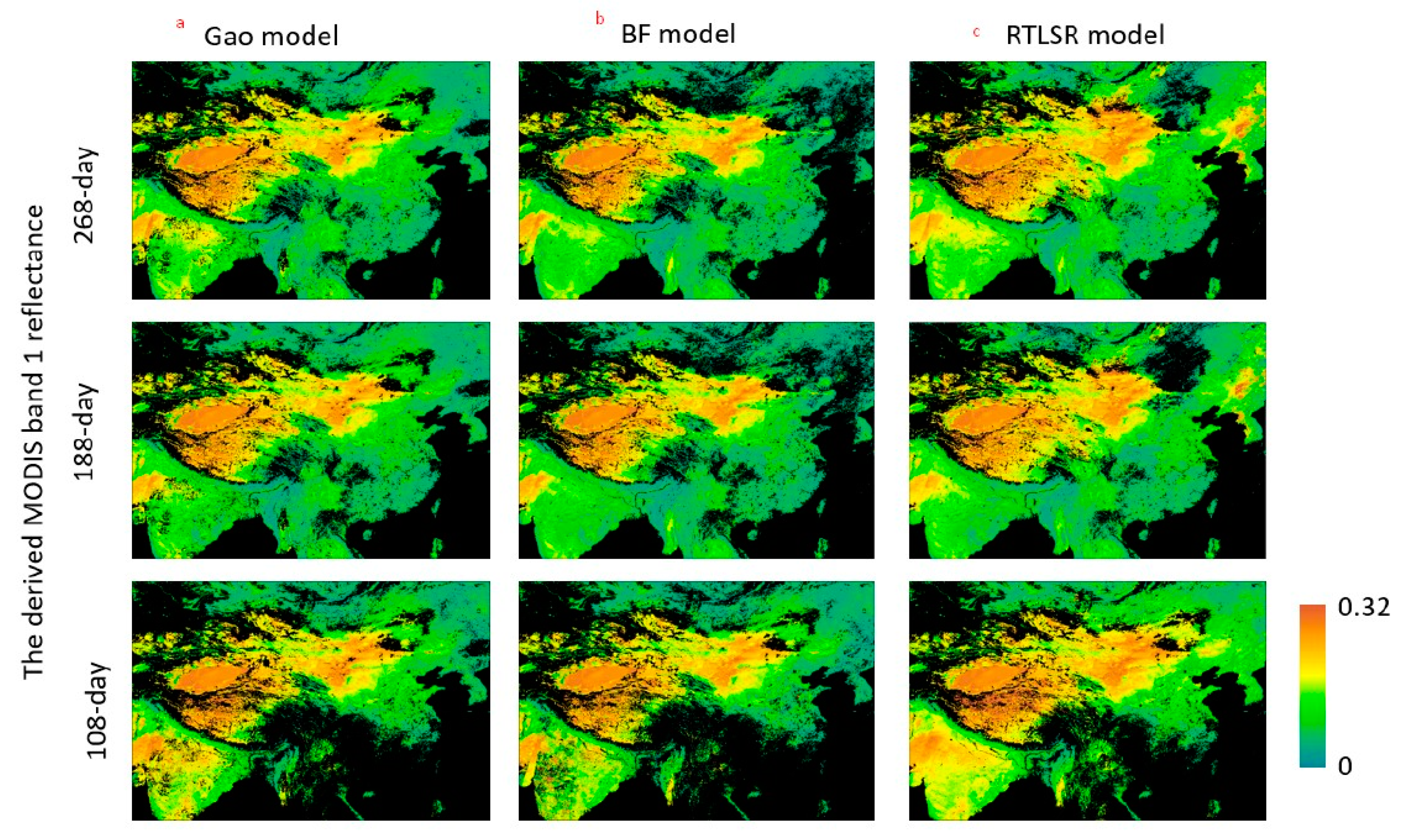
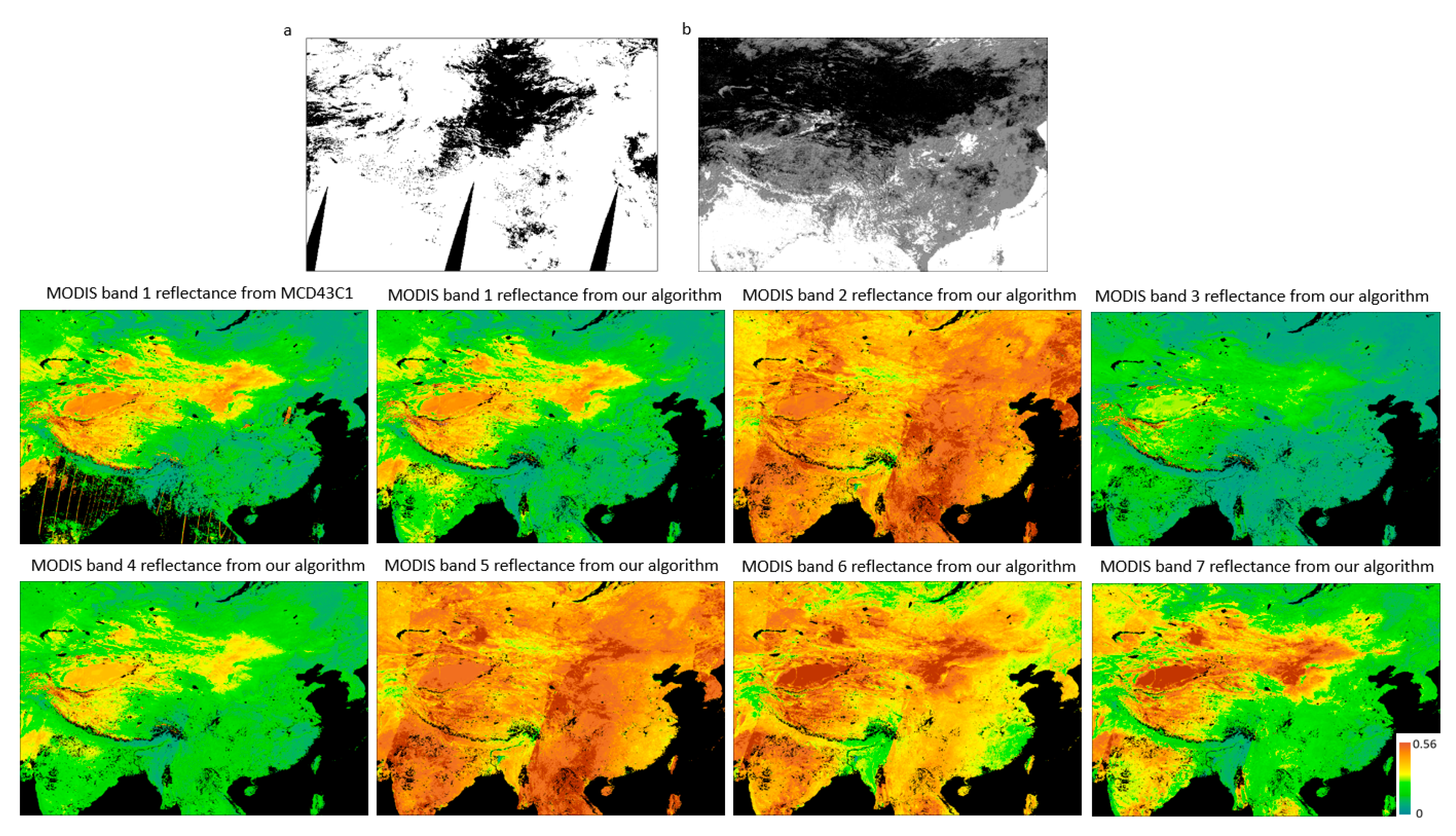
4.1. Retrieval of MODIS Band Reflectance Based on the BRDF Models

The retrieval was performed based on the three models (e.g., RTLSR model, Gao model, and adjusted BF model) for different inversion periods (e.g., 108 days, 188 days, and 268 days) from 2012 to 2015. First, we selected the derived MODIS band-1 reflectance on the 216th day of the year in 2012 as an example to analyze the performance efficiency of the models (see Figure 3).

Compared with the results in Figure 3, we find that the results based on the RTLSR model have the most valid retrieval instances for all inversion periods, followed by those of the adjusted BF model and the Gao model. Adding the model parameters is a main reason for the decrease in the performance efficiency, as more input datasets for are required retrieval. However, the differences in the numbers of valid retrievals among the three models can be minimized when the inversion period is sufficiently long (e.g., 268 days; see first line of Figure 3). For the spatial continuity, the three models have similar behaviors, and the inversion period is sufficiently long. In addition to the derived MODIS band-1 reflectance based on the three models, the MODIS bands 2–7 reflectance in East and South Asia in 2012 was also derived; and the variation of spatial continuity of the MODIS bands 2–7 retrieval derived within the three inversion periods is similar to that of MODIS band-1 retrieval.

After showing the spatial variation of the valid retrieval based on the three models for the three inversion periods, the valid retrieval precision for MODIS band 1–7 are carried out. Obvious differences in the mean RMSE% can be observed among the three models (e.g., 6.6–64.1% for the RTLSR model, 5.3–52.8% for the adjusted BF model, and 5.3–27.7% for the Gao model; see

Table 2. Precision (RMSR%) statistic for the daily mean RMSE% of the time series for the derived MODIS bands 1–7 and shortwave band in 2012

Band		Band 1	Band 2	Band 3	Band 4	Band 5	Band 6	Band 7	Shortwave
Bandwidth (NM)		620–670	841–876	459–479	545–565	1230–1250	1628–1652	2105–2155	400–2500
268 day	RTLSR	34.6	18.9	64.1	40.4	8.2	10.9	16.4	19.6
	Gao	16.7	11.4	27.7	18.3	7.0	7.6	11.0	9.8
	Adjusted BF	26.3	16.5	52.8	33.1	7.1	9.3	12.9	16.4
188 day	RTLSR	34.4	16.6	53.8	33.8	7.6	9.6	14.6	17.9
	Gao	15.5	10.7	26.6	17.2	6.5	7.0	9.9	9.7
	Adjusted BF	25.1	13.7	44.0	27.7	6.4	7.7	10.7	14.7
108 day	RTLSR	28.0	14.4	45.8	28.7	6.6	8.3	12.3	15.4
	Gao	13.8	9.3	24.2	15.6	5.7	6.2	8.7	9.7
	Adjusted BF	19.2	10.6	36.2	22.8	5.3	6.5	8.9	12.5

). Although the Gao model is seemingly optimal based on the above results, it is difficult to determine whether the models reach acceptable precision compared with those in previous research on the validation of shortwave albedo [4,43,44].

The time series of the daily mean MODIS band 1–7 reflectance within no-cloud MODIS pixels in 2012 is yielded (see Figure 4), which shows that Gao model is nearest to no-cloud MODIS observation while the inversion period being enough long; and the quantitative statistic (e.g., bias seeing lower right Figure 4) also verifies the aforementioned results.

In other words, expanding the inversion period can minimize the difference in model performance efficiency and may result in retrieval with unstable precision. The precision of the models requires further evaluation. The detailed analysis and discussion of the precision of the BRDF models highlight the reliability of each model and differences among models under the different inversion conditions in Section 5.1 and Section 5.2.

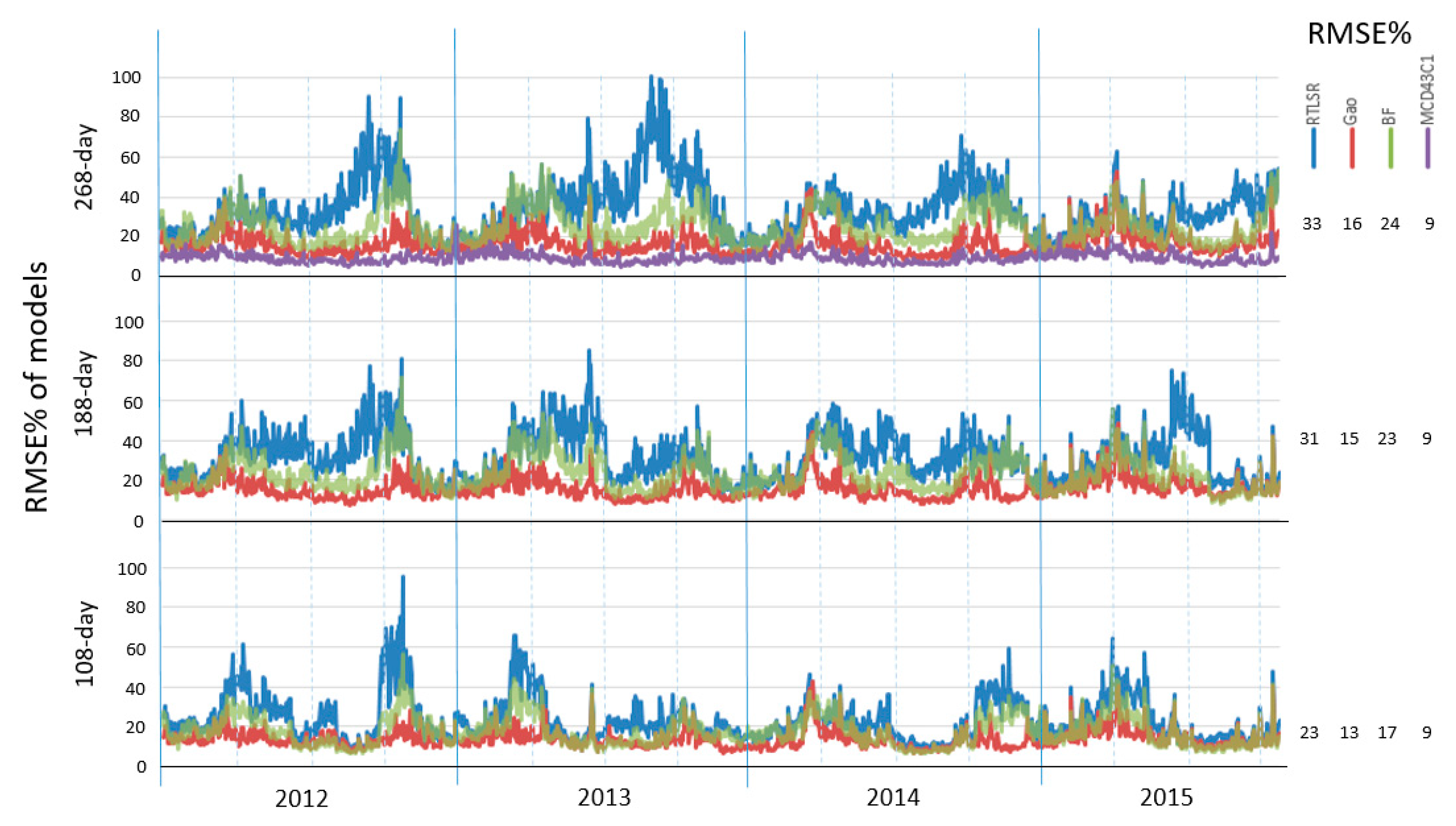
4.2. Performance in the Reconstruction of Spatiotemporally Continuous MODIS-Band Reflectance

In this section, we implemented the proposed filling algorithm to reconstruct spatiotemporally continuous MODIS-band reflectance according to the flowchart in Section 2. In addition, a dataset of spatiotemporally continuous MODIS-band reflectance is reconstructed, and it includes the derived MODIS band 1–7 reflectance from 2012 to 2015 in East and South Asia. An example is shown in Figure 5.

The results in Figure 5, as an example, shows a seemingly rational spatial distribution, particularly in the southwest part of China (e.g., the part of Sichuan Province and in the Yunnan–Guizhou Plateau region) and in southern Asia including the South Asian Sub-Continent and Southeast Asia, in which clouds are predominant for the majority of months of the year. For the derived MODIS band-1 reflectance calculated from the MCD43C1 V006 parameters in Figure 5, there are many abnormal values in Sichuan Province, the Yunnan–Guizhou Plateau region, South Asia and Southeast Asia because filling and even invalid values are used. The reconstructed MODIS-band 1–7 reflectance result displays optimal spatial continuity and an acceptable spatial distribution (Figure 5).

Considering the aforementioned validation process, we believe that the reconstruction method for MODIS-band reflectance in the aforementioned area provides acceptable precision.

5. Discussion

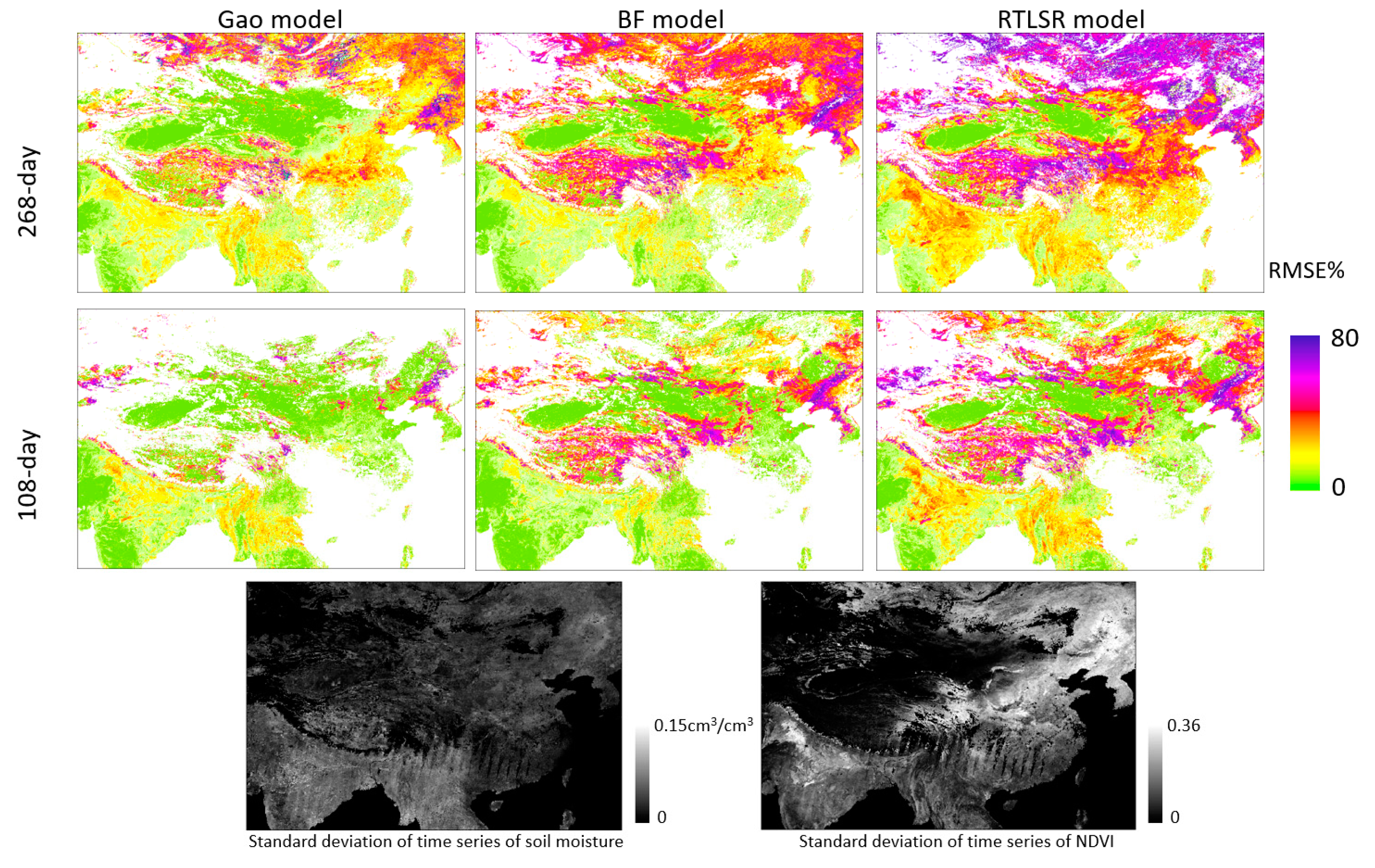
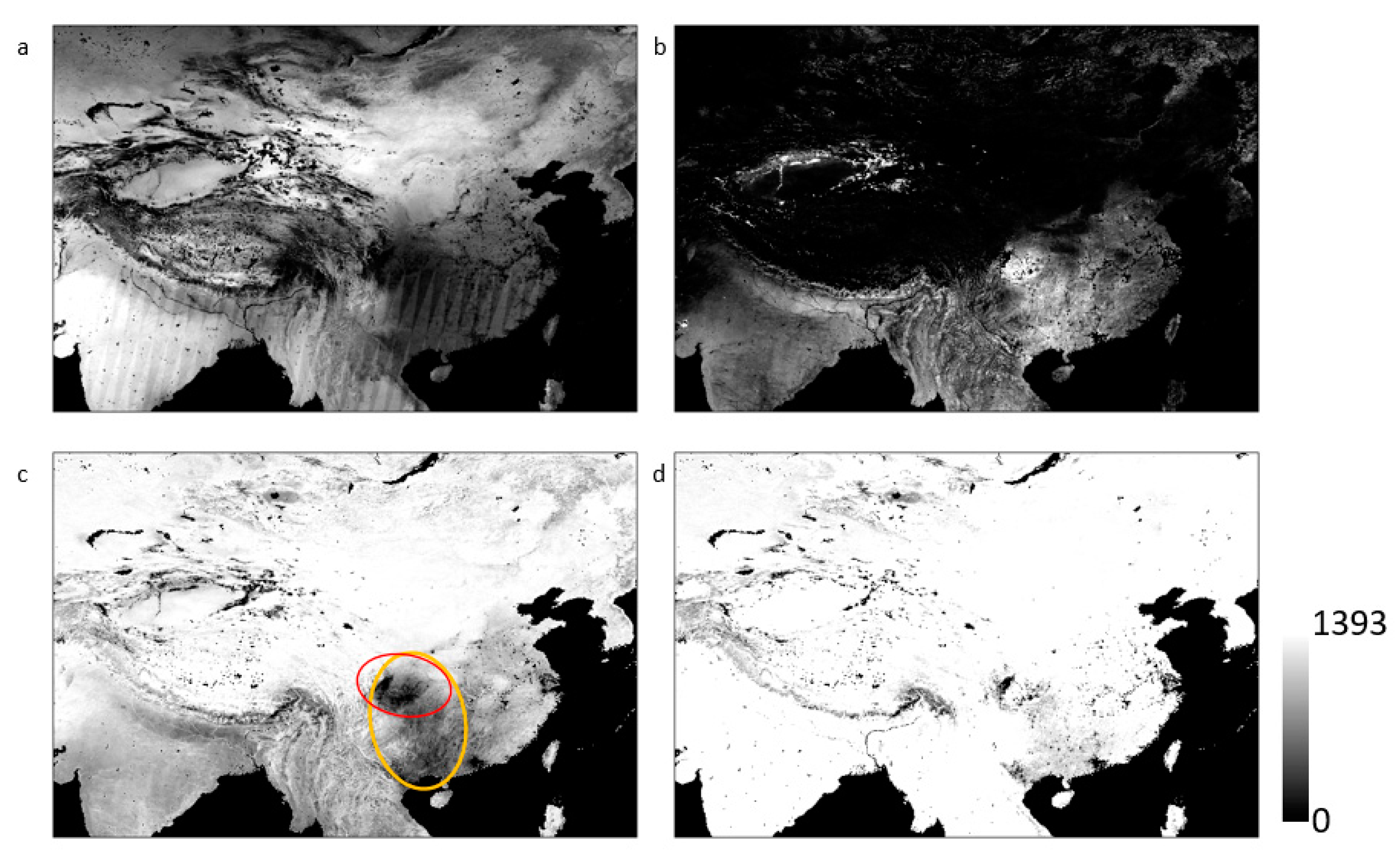
5.1. Spatiotemporal Distribution of the Precision of the Derived MODIS Band Reflectance based on the BRDF Models

In theory, the Gao model and adjusted BF model should become increasingly accurate when the inversion period is sufficiently long (e.g., 268 days) [4,34]. The derived parameters of the Gao model and adjusted BF model are dynamic and can accurately describe the variations in land surface construction; this is an advantage of the Gao and adjusted BF models compared to the RTLSR model.

In Figure 6, the success rate of the retrieval increases as the inversion period expands; and the RTLSR model has the most valid retrieval, the main reason is that the added BRDF parameter for the Gao and adjusted BF models increases the threshold for retrieval; for example, more than 8, more than 10, and more than 10 observations are used in the derivations of the RTLSR model, adjusted BF model and Gao model, respectively [7,34]. In the meantime, The adjusted BF model adds the NDVI to the RTLSR model as an intermediate variable, and the Gao model introduces both the NDVI and soil moisture into the RTLSR model to consider changes in land surface attributes; which results in the better precision of the Gao and adjusted BF models compared with the RTLSR model (see Table 2 and Figure 4). Some interesting phenomenon in Figure 3, Unlike the results at latitudes south of the 35th parallel, is that the validity of retrieval does not increase with the inversion period at latitudes north of the 35th parallel, mainly for two reasons: 1) there are so few clouds that the retrieval can be easily performed for any inversion period from 108 days to 268 days, and 2) invalid retrievals are caused by the input datasets with land cover changes over long inversion periods. For example, the result on the 216th day of the year in 2012 was derived based on time series from the 82th day to 349th day of the year in 2012, and snow is common each year after September in North Asia.

By comparing the three models further (see Figure 6), we can see the different precisions of the time series of the derived MODIS band-1 reflectance for different inversion periods. Notably, the Gao model is optimal and stable, with an RMSE% that fluctuates from 13% to 16%; the adjusted BF model is moderately accurate, and the RMSE% ranges from 17% to 23%; and the RTLSR model performs worst, with an RMSE% ranging from more than 23% to 33%; the aforementioned statistic is shown at the right side of Figure 6. These results further verify that the dynamic parameters in the Gao model and adjusted BF model can describe bidirectional reflectance with better precision than that based on the fixed parameters in the RTLSR model. Therefore, we believe that the retrievals based on the Gao model and adjusted BF model can be effective in areas covered by long-term clouds, such as the region south of the Yangtze River in Asia. Further analysis of the results suggests that low-precision retrievals occur at the ends of the first and third quarters every year, when the snow season ends and begins, respectively; moreover, the input datasets may have different land cover characteristics, such as vegetation in the growing season and snow in the winter.

For comparison, the derived MODIS band-1 reflectance from the MCD43C1 V006 full inversion is shown in Figure 6 (purple); the RMSE% fluctuates around approximately 10%, and the mean RMSE% ranges from 9% to 10%, which can be regarded as an acceptable precision standard considering the widespread land uses, the algorithm assumptions (e.g., 16-day inversion period and the observations from both the Terra and Aqua satellites) and the high quality of the input dataset (e.g., using the snow status weighted for the ninth day instead of the majority of the snow/no-snow observations from the 16-day period, as continually updated based on archetypal BRDF) [4,22].

The validation is expanded from MODIS band 1 (see Figure 6) to MODIS bands 2–7 (see

Table 3. Precision statistic for the daily mean RMSE% of the time series for the derived MODIS bands 1–7 and shortwave band from 2012 to 2015

		Band 1	Band 2	Band 3	Band 4	Band 5	Band 6	Band 7
	Bandwidth (NM)	620–670	841–876	459–479	545–565	1230–1250	1628–1652	2105–2155
268 day	MCD43C1	9.6	6.7	21.4	14.0	5.2	5.4	8.5
	RTLSR	33.8	18.1	60.7	39.0	8.1	10.4	21.6
	Gao	16.7	11.6	28.1	18.4	7.1	7.6	12.8
	Adjusted BF	24.9	15.4	49.4	31.1	7.0	8.8	17.3
188 day	MCD43C1	9.5	6.7	21.3	13.9	5.1	5.4	7.3
	RTLSR	31.3	16.8	54.5	34.5	7.5	9.7	14.7
	Gao	15.7	10.7	26.7	17.3	6.6	7.1	10.0
	Adjusted BF	23.2	13.4	44.1	27.7	6.3	7.9	10.9
108 day	MCD43C1	9.3	6.5	20.2	13.3	5.1	5.3	7.2
	RTLSR	23.2	13.9	42.3	26.7	6.5	8.2	12.1
	Gao	13.7	9.1	23.6	15.3	5.6	6.2	8.6
	Adjusted BF	17.5	10.2	34.2	21.5	5.2	6.4	8.8

); compared with Table 2, the precision is calculated from 2012 to 2015, and the results from MCD43C1 V006 are introduced as a benchmark. Obviously, the RMSE% of Gao model shows the better precision, and is nearer to that of MCD43C1 V006 at all MODIS band than that of the adjusted BF model and RTLSR model.

We further analyze the spatial distribution of the precision of the models. The RMSE% values of the time series of the derived MODIS band-1 reflectance based on the three models are shown pixel by pixel in Figure 7. In addition to the number of valid retrievals increases with increasing inversion period, and we find that the Gao and adjusted BF models provide high precision in areas where many MODIS pixels are filled have no values for MCD43C1 V006; for example, in the Yunnan–Guizhou Plateau region and south of the Yangtze River, South Asia, and Southeast Asia (see Figure 2). Because the aforementioned areas are located in the subtropical monsoon region with long-term clouds, the number of input datasets is insufficient for triggering retrieval in short periods with stable land cover states (e.g., 16 days) [7].

Besides the aforementioned discussions, an interesting analysis is introduced by comparison of the difference in the spatiotemporal distribution of the AFX derived by BRDFs’ parameters at MODIS band-1 reflectance on the 80th day and 216th day of the year in 2012 (see Figure 8) based on the AFX equation (Equation (6)) [29].

$$AFX=1+0.189184\times F_v-1.377622\times F_g$$

(6)

and,

$$\begin{array}{l}{F}_v=f_{vol}/fiso,F_g=f_{geo}/fiso\hspace{1em}\hspace{1em}\mathrm{for} \mathrm{RTLSR} \mathrm{model}\\ F_v=f_{vol\_n}/fiso,F_g=f_{geo\_n}/fiso \mathrm{for} \mathrm{Adjusted} \mathrm{BF} \mathrm{model}\\ F_v=f_{vol\_ns}/fiso,F_g=f_{geo\_ns}/fiso \mathrm{for} \mathrm{Gao} \mathrm{model}\end{array}$$

AFX, as a combination of normalized BRDF parameters, indicates which one of geometric optical scattering and volumetric scattering dominates the anisotropic reflectance of BRDF [28,29]. Comparison of AFX derived by the BRDF models may be interesting and surprising for evaluating the precision of the BRDF models. For Gao model, we find that lots of AFX is less than 1st on 216th day of the year in 2012, which means geometric optical scattering is dominated; there are lots of AFX more than 1 on 80th day of the year in 2012, which means volumetric scattering dominates in the area highlighted by purple color (see first sample of Figure 8). The variation of Adjusted BF model is similar to Gao model (see second sample in Figure 8). We judge that the phenological change of the vegetation results in the aforementioned variation of AFX spatial distribution, because the experiment area is located in the subtropical monsoon region, and covered by kinds of vegetation. However, the spatial distribution variation of AFX derived by RTLSR model is subtle, compared with the other two model, which is obviously incorrect; and the too long inversion period (e.g., 268-day inversion period) for RTLSR model is main reason.

The other one phenomenon is that AFX legend ranges from −0.5 to 2, which is seemingly unreasonable; and a range from 0 to 2 may be right by comparing with the previous research [28]. We find the low AFX near to −0.5 spread at latitudes north of the 35th parallel, which is caused by the low-accuracy retrieval, for example, the input datasets with land cover changes over long inversion periods. A specific explanation has shown in the beginning of Section 5.1. In the meantime, there are the least retrieval with AFX near to −0.5 for Gao model; which means soil moisture may restrain the retrieving error caused by the changing land cover, for example, from vegetation to snow at latitudes north of the 35th parallel.

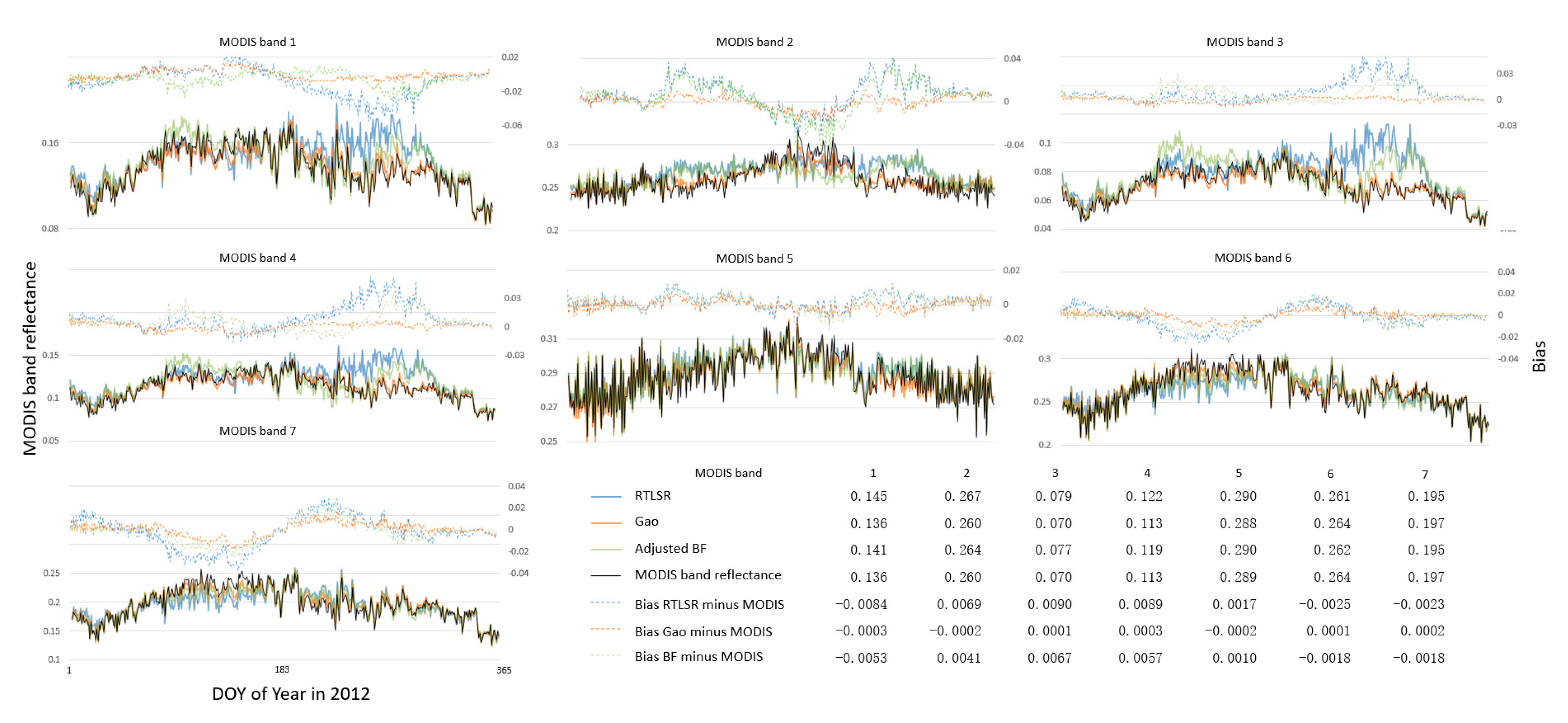
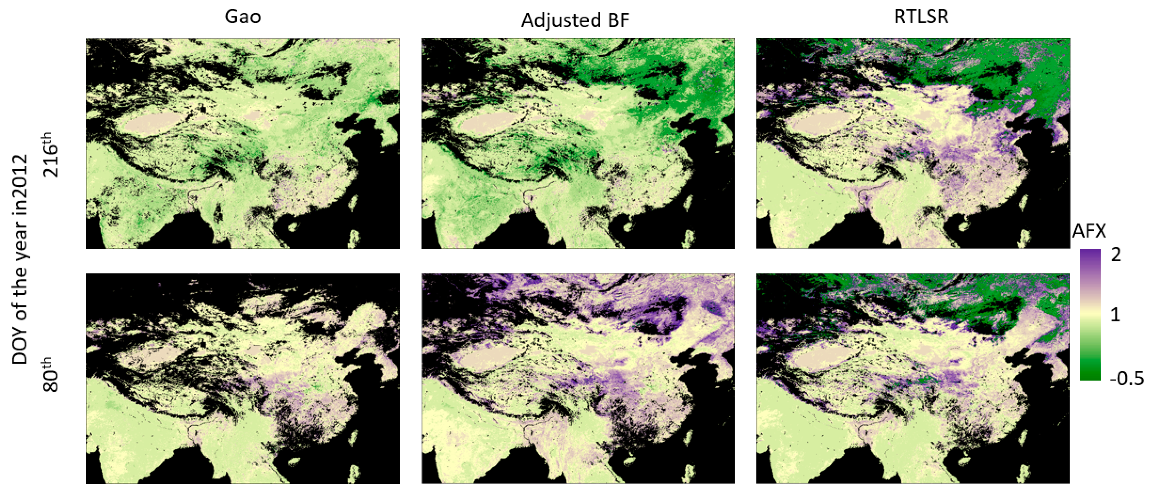
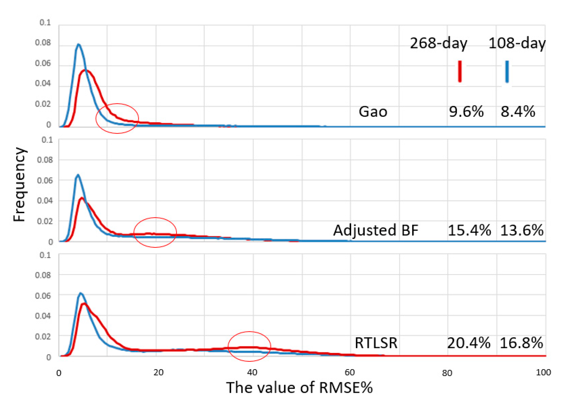
5.2. Evaluation of Derived Shortwave Reflectance based on the Three BRDF Models

Although most valid retrievals based on the Gao model and adjusted BF model can be performed at precision levels superior to those of the RTLSR model for long inversion periods, there is a lack of comparable research on the validation of MODIS band reflectance. In previous research, the retrieved shortwave albedo products displayed different precision levels for different algorithms, different remotely sensed observations, different sites with different land cover properties, and other factors at shortwave band [4,45,46,47].

To comprehensively evaluate the Gao model and adjusted BF model, we introduced the derived MODIS 1–7 band reflectances in 2012 (see Table 2 and Table 3). The derived MODIS 1–7 band reflectance values have inconsistent precision, so it is difficult to determine if the precision is acceptable (see Table 2 and Table 3). Therefore, a conversion from MODIS-band reflectance to shortwave reflectance was performed based on the method proposed by Liang [48].

$${\rho }_{}({\theta }_i,{\theta }_v,{\varphi }_i,{\varphi }_v)={\displaystyle \underset{0.4\mu m}{\overset{2.5\mu m}{\int }}w(\lambda )\rho ({\theta }_i,{\theta }_v,{\varphi }_i,{\varphi }_v,\lambda )}d\lambda ={\displaystyle \sum _l{w}_l{\rho }_l\left({\theta }_i,{\theta }_v,{\varphi }_i,{\varphi }_v,\lambda \right)}$$

(7)

where ρ is the broadband shortwave land surface reflectance; w is the weighing coefficient of each band for converting narrowband to broadband (NTOB) shortwave land surface reflectance; and l is the number of bands.

In addition, MODIS band 1–7 reflectance values from MODIS observations and derived by the three models are used to convert NTOB shortwave land surface reflectance data (

Table 4. Converting weights for NTOB MODIS reflectance [48].

	Band 1	Band 2	Band 3	Band 4	Band 5	Band 6	Band 7	Shortwave
Bandwidth (NM)	620–670	841–876	459–479	545–565	1230–1250	1628–1652	2105–2155	400–2500
MODIS	0.3973	0.2382	0.3489	−0.2655	0.1604	−0.0138	0.0682	0.0036

). The resulting histograms show that the precision of the derived land surface reflectance based on the models varies. From the histograms (see Figure 9), when the inversion period expands from 108 days to 268 days, the RMSE% results of the Gao model plot between 5% and 10%, and those of the adjusted BF model and RTLSR model shift upward (e.g., by 20% for the adjusted BF model and 40% for the RTLSR model). In Figure 9, the red circle denotes the shift which quantifies the ability of models restraining the retrieving error while the inversion period expanding. Obviously, The RMSE% of the Gao model is always best with no more than 10%, and that of the adjusted BF ranging from 13.6% to 15.4% comes second, which corresponds to the features of the “shortwave” column in Table 2.

By comparing with the previous research, for example, Qu et al. retrieved shortwave albedo with an RMSE of 0.0538 at 53 sites; Shuai et al. reported retrievals with RMSEs of 0.025 and 0.016 RMSE values for MODIS-representative and Landsat-representative sites, respectively; and other validations have reported similar precision levels [46,47]. In this case, the precision of the Gao model and adjusted BF model is acceptable for long inversion periods. We verified that the Gao model, as the main model in the filling algorithm, has acceptable precision for filling MODIS cloudy pixels. For the RTLSR model, the BRDF parameters from MCD43C1 V006 were adopted for filling cloudy MODIS pixels with QA values ranging from 0 to 4 in the proposed filling algorithm; in such a case, the Gao model and adjusted BF model are complementary to the RTLSR model.

5.3. Quantification of the Improvement in Spatiotemporal Continuity for the Reconstruction of MODIS-Band Reflectance

From the above example, we compare the difference in the spatial distribution of MODIS-band reflectance from MCD43C1 V006 and our proposed algorithm; obviously, the reconstruction based on the proposed algorithm has better spatial continuity than that of MCD43C1 V006. Furthermore, we show the number of days with clouds (Figure 2c) based on MCD43C1 V006 and the proposed algorithm (see Figure 10). In the whole experimental area, there are approximately 30.3% no-cloud MODIS observations. After being processed by MCD43C1 V006 BRDF, no-cloud MODIS observations reach approximately 90.5% of all observations. However, the proposed algorithm removes 7.6% of the cloudy MODIS pixels based on the MCD43C1 V006 product. Thus, the reconstructed MODIS-band reflectance has greater than 98% spatiotemporal coverage.

If we further calculate the improvement in spatiotemporal continuity in the Yunnan–Guizhou Plateau, Sichuan Province, and Guangxi Province regions, for which MCD43C1 V006 adopts many filled and invalid values, the spatiotemporal coverage of MODIS-band reflectance derived from MCD43C1 V006 reaches 62.6% (see the yellow circle in Figure 10); with our proposed algorithm, the spatiotemporal coverage of MODIS-band reflectance reaches nearly 90.7%. In Sichuan Province (see the red circle in Figure 10), the proposed algorithm provides 87.4% spatiotemporal continuity for MODIS-band reflectance, which is obviously superior to that of MCD43C1 V006 (e.g., 59.3%).

6. Conclusions

To address the issue of poor spatiotemporal continuity for remotely sensed observations due to cloud cover, we proposed a filling algorithm that combines the aforementioned three BRDF models to derive the no-cloud MODIS-band reflectance in Asia from 2012 to 2015 with improved precision (e.g., no more than 10% for the Gao model and 12.5–16.4% for the adjusted BF model at shortwave band, see Table 2). In this approach, the MODIS-band reflectance values that are filled or invalid are replaced with values from MCD43C1 V006, and no-cloud MODIS-band reflectance with a reasonable spatial distribution is obtained (see Figure 10). Additionally, the reconstructed MODIS-band reflectance has a spatiotemporal coverage greater than 98%, with improvements of more than 28% in Sichuan Province and on the Yunnan–Guizhou Plateau. Due to the limitations of the spatial coverage of the input parameter (e.g., soil moisture), we only reconstructed MODIS-band reflectance with a high spatiotemporal continuity in East and South Asia; based on the aforementioned result, we believe that the spatiotemporal continuity of MODIS-band reflectance can be improved significantly at low latitudes by the proposed algorithm.

In addition, we further analyzed the three models and determined that the RTLSR model is a basic BRDF model with good precision, a short inversion period and strict quality control (e.g., MCD43C1 V006) [4,49], thus providing an optimal option for filling cloudy MODIS pixels. The Gao model and adjusted BF model use dynamic parameters to reflect the changing land surface and can provide acceptable precision for derived land surface reflectance when the inversion period is sufficiently long (e.g., 108 days, 188 days, or 268 days); these models perform evidently better than the RTLSR model. Moreover, the Gao model is superior to the adjusted BF model based on precision on account of the considered theoretical mechanism, and this finding was similar to that in previous research [34]. The aforementioned work further verifies the reasonability of the Gao model. We find that it is difficult to accurately describe the temporal variations in land surface reflectance when using only the NDVI and ignoring soil moisture.

Additional work is needed to improve this type of research in the future. Areas in which the spatiotemporal coverage is low in derived data sets must be assessed, for example, the coverage is 90% or lower in Sichuan Province. Artificial intelligence methods may be a good choice for future work to increase the spatiotemporal coverage of input parameters (e.g., NDVI and soil moisture) that are important in the current methods to achieve good spatiotemporal continuity. The above topics will be considered in future research.

References

1. Wulder, M.A.; Loveland, T.R.; Roy, D.P.; Crawford, C.J.; Masek, J.G.; Woodcock, C.E.; Allen, R.G.; Anderson, M.C.; Belward, A.S.; Cohen, W.B.; et al. Current status of Landsat program, science, and applications. Remote Sens. Environ. 2019, 225, 127–147. [Google Scholar] [CrossRef]
2. Vermote, E.; Justice, C.; Claverie, M.; Franch, B. Preliminary analysis of the performance of the Landsat 8/OLI land surface reflectance product. Remote Sens. Environ. 2016, 185, 46–56. [Google Scholar] [CrossRef] [PubMed]
3. Claverie, M.; Vermote, E.; Franch, B.; Masek, J.G. Evaluation of the Landsat-5 TM and Landsat-7 ETM+ surface reflectance products. Remote Sens. Environ. 2015, 169, 390–403. [Google Scholar] [CrossRef]
4. Mira, M.; Weiss, M.; Baret, F.; Courault, D.; Hagolle, O.; Gallego-Elvira, B.; Olioso, A. The MODIS (collection V006) BRDF/albedo product MCD43D: Temporal course evaluated over agricultural landscape. Remote Sens. Environ. 2015, 170, 216–228. [Google Scholar] [CrossRef] [Green Version]
5. Huete, A.; Didan, K.; Miura, T.; Rodriguez, E.P.; Gao, X.; Ferreira, L.G. Overview of the radiometric and biophysical performance of the MODIS vegetation indices. Remote Sens. Environ. 2002, 83, 195–213. [Google Scholar] [CrossRef]
6. Wang, T.; Shi, J.; Yu, Y.; Husi, L.; Gao, B.; Zhou, W.; Ji, D.; Zhao, T.; Xiong, C.; Chen, L. Cloudy-sky land surface longwave downward radiation (LWDR) estimation by integrating MODIS and AIRS/AMSU measurements. Remote Sens. Environ. 2018, 205, 100–111. [Google Scholar] [CrossRef]
7. Schaaf, C.B.; Gao, F.; Strahler, A.H.; Lucht, W.; Li, X.; Tsang, T.; Strugnell, N.C.; Zhang, X.; Jin, Y.; Muller, J.P. First operational BRDF, albedo nadir reflectance products from MODIS. Remote Sens. Environ. 2002, 83, 135–148. [Google Scholar] [CrossRef] [Green Version]
8. Zhou, J.; Jia, L.; Menenti, M. Reconstruction of global MODIS NDVI time series: Performance of Harmonic ANalysis of Time Series (HANTS). Remote Sens. Environ. 2015, 163, 217–228. [Google Scholar] [CrossRef]
9. Tavakol, A.; Rahmani, V.; Quiring, S.M.; Kumar, S.V. Evaluation analysis of NASA SMAP L3 and L4 and SPoRT-LIS soil moisture data in the United States. Remote Sens. Environ. 2019, 229, 234–246. [Google Scholar] [CrossRef]
10. Justice, C.; Townshend, J.; Vermote, E.; Masuoka, E.; Wolfe, R.; Saleous, N.; Roy, D.; Morisette, J. An overview of MODIS Land data processing and product status. Remote Sens. Environ. 2002, 83, 3–15. [Google Scholar] [CrossRef]
11. Pekel, J.F.; Cottam, A.; Gorelick, N.; Belward, A.S. High-resolution mapping of global surface water and its long-term changes. Nature 2016, 540, 418–422. [Google Scholar] [CrossRef] [PubMed]
12. Tao, S.; Fang, J.; Ma, S.; Cai, Q.; Xiong, X.; Tian, D.; Zhao, X.; Fang, L.; Zhang, H.; Zhu, J. Changes in China’s lakes: Climate and human impacts. Natl. Sci. Rev. 2020, 7, 132–140. [Google Scholar] [CrossRef] [Green Version]
13. Ronghua, M. A half-century of changes in China’s lakes: Global warming or human influence? Geophysical Research Letters 2010. [Google Scholar] [CrossRef]
14. Wang, M.; Du, L.; Ke, Y.; Huang, M.; Zhang, J.; Zhao, Y.; Li, X.; Gong, H. Impact of Climate Variabilities and Human Activities on Surface Water Extents in Reservoirs of Yongding River Basin, China, from 1985 to 2016 Based on Landsat Observations and Time Series Analysis. Remote Sens. 2019, 11, 560. [Google Scholar] [CrossRef] [Green Version]
15. Zhang, G.; Yao, T.; Chen, W.; Zheng, G.; Shum, C.K.; Yang, K.; Piao, S.; Sheng, Y.; Yi, S.; Li, J. Regional differences of lake evolution across China during 1960s-2015 and its natural and anthropogenic causes. Remote Sens. Environ. 2018, 221, 386–404. [Google Scholar] [CrossRef]
16. Cover, M.L.; Change, L.-C. MODIS Land Cover Product Algorithm Theoretical Basis Document (ATBD) Version 5.0; 1999. Available online: https://modis.gsfc.nasa.gov/data/atbd/atbd_mod12.pdf (accessed on 5 November 2020).
17. Cui, Y.; Zeng, C.; Zhou, J.; Xie, H.; Wan, W.; Hu, L.; Xiong, W.; Chen, X.; Fan, W.; Hong, Y. A spatio-temporal continuous soil moisture dataset over the Tibet Plateau from 2002 to 2015. Sci. Data 2019, 6, 1–7. [Google Scholar] [CrossRef] [Green Version]
18. Gao, F.; Anderson, M.; Daughtry, C.; Johnson, D. Assessing the variability of corn and soybean yields in central Iowa using high spatiotemporal resolution multi-satellite imagery. Remote Sens. 2018, 10, 1489. [Google Scholar] [CrossRef] [Green Version]
19. Lin, C.H.; Lai, K.H.; Chen, Z.B.; Chen, J.Y. Patch-Based Information Reconstruction of Cloud-Contaminated Multitemporal Images. IEEE Trans. Geosci. Remote. Sens. 2014, 52, 163–174. [Google Scholar] [CrossRef]
20. Wan, Z.; Li, Z.-L. A physics-based algorithm for retrieving land-surface emissivity and temperature from EOS/MODIS data. IEEE Trans. Geosci. Remote. Sens. 1997, 35, 980–996. [Google Scholar]
21. Huete, A.; Justice, C.; Van Leeuwen, W. MODIS vegetation index (MOD13). In Algorithm Theor. Basis Doc.; 1999; 4. Available online: https://modis.gsfc.nasa.gov/data/atbd/atbd_mod13.pdf (accessed on 5 November 2020).
22. Strahler, A.H.; Muller, J.; Lucht, W.; Schaaf, C.; Tsang, T.; Gao, F.; Li, X.; Lewis, P.; Barnsley, M.J. MODIS BRDF/albedo product: Algorithm theoretical basis document version 5.0. MODIS Doc. 1999, 23, 42–47. [Google Scholar]
23. Tang, X.; Bullock, E.L.; Olofsson, P.; Woodcock, C.E. Can VIIRS continue the legacy of MODIS for near real-time monitoring of tropical forest disturbance. Remote Sens. Environ. 2020, 249, 112024. [Google Scholar] [CrossRef]
24. Strugnell, N.C.; Lucht, W.; Hyman, A.H.; Meister, G. Continental-scale albedo inferred from land cover class, field observations of typical BRDFs and AVHRR data. In Proceedings of the IGARSS’98. Sensing and Managing the Environment. 1998 IEEE International Geoscience and Remote Sensing. Symposium Proceedings, (Cat. No. 98CH36174), Seattle, WA, USA, 6–10 July 1998; pp. 595–597. [Google Scholar]
25. Strugnell, N.C.; Lucht, W. An algorithm to infer continental-scale albedo from AVHRR data, land cover class, and field observations of typical BRDFs. J. Clim. 2001, 14, 1360–1376. [Google Scholar] [CrossRef]
26. Vermote, E.; Justice, C.O.; Bréon, F.-M. Towards a generalized approach for correction of the BRDF effect in MODIS directional reflectances. IEEE Trans. Geosci. Remote. Sens. 2008, 47, 898–908. [Google Scholar] [CrossRef]
27. Zhang, H.; Jiao, Z.T.; Chen, L.; Dong, Y.D.; Zhang, X.N.; Lian, Y.; Qian, D.; Cui, T.J. Quantifying the Reflectance Anisotropy Effect on Albedo Retrieval from Remotely Sensed Observations Using Archetypal BRDFs. Remote Sens. 2018, 10, 1628. [Google Scholar] [CrossRef] [Green Version]
28. Zhang, H.; Jiao, Z.T.; Dong, Y.D.; Du, P.; Li, Y.; Lian, Y.; Cui, T.J. Analysis of Extracting Prior BRDF from MODIS BRDF Data. Remote Sens. 2016, 8, 1004. [Google Scholar] [CrossRef] [Green Version]
29. Jiao, Z.T.; Hill, M.J.; Schaaf, C.B.; Zhang, H.; Wang, Z.S.; Li, X.W. An Anisotropic Flat Index (AFX) to derive BRDF archetypes from MODIS. Remote Sens. Environ. 2014, 141, 168–187. [Google Scholar] [CrossRef]
30. Franch, B.; Vermote, E.F.; Sobrino, J.A.; Julien, Y. Retrieval of Surface Albedo on a Daily Basis: Application to MODIS Data. IEEE Trans. Geosci. Remote. Sens. 2014, 52, 7549–7558. [Google Scholar] [CrossRef]
31. Franch, B.; Vermote, E.F.; Claverie, M. Intercomparison of Landsat albedo retrieval techniques and evaluation against in situ measurements across the US SURFRAD network. Remote Sens. Environ. 2014, 152, 627–637. [Google Scholar] [CrossRef]
32. Franch, B.; Vermote, E.; Skakun, S.; Roger, J.; Masek, J.G.; Ju, J.; Villaescusanadal, J.L.; Santamariaartigas, A. A Method for Landsat and Sentinel 2 (HLS) BRDF Normalization. Remote Sens. 2019, 11, 632. [Google Scholar] [CrossRef] [Green Version]
33. Franch, B.; Vermote, E.; Skakun, S.; Roger, J.C.; Santamaria-Artigas, A.; Villaescusa-Nadal, J.L.; Masek, J. Toward Landsat and Sentinel-2 BRDF Normalization and Albedo Estimation: A Case Study in the Peruvian Amazon Forest. Front. Earth Sci. 2018, 6. [Google Scholar] [CrossRef] [Green Version]
34. Gao, B.; Gong, H.; Wang, T.; Zhou, J. An Improved Bidirectional Reflectance Distribution Function (BRDF) Model that Considers Soil Moisture and the Normalized Difference Vegetation Index (NDVI). IEEE Trans. Geosci. Remote. Sens. 2020. (under review). [Google Scholar]
35. Zeng, J.Y.; Chen, K.S.; Bi, H.Y.; Chen, Q. A Preliminary Evaluation of the SMAP Radiometer Soil Moisture Product Over United States and Europe Using Ground-Based Measurements. IEEE Trans. Geosci. Remote. Sens. 2016, 54, 4929–4940. [Google Scholar] [CrossRef]
36. Roujean, J.L. A bidirectional reflectance model of the Earth’s surface for the correction of remote sensing data. J. Geophys. Res. 1992, 97, 20455–420468. [Google Scholar] [CrossRef]
37. Schaaf, C.B.; Strahler, A.H. Solar Zenith Angle Effects on Forest Canopy Hemispherical Reflectances Calculated with a Geometric-Optical Bidirectional Reflectance Model. IEEE Trans. Geosci. Remote. Sens. 1993, 31, 921–927. [Google Scholar] [CrossRef]
38. Schaaf, C.B.; Strahler, A.H. Simulating the Bidirectional and Hemispherical Reflectance of Mountainous and Forested Scenes with a Geometric-Optical Model. In Proceedings of the Seventh Conference on Satellite Meteorology and Oceanography, Monterey, CA, USA, 6–10 June 1994; pp. 602–604. [Google Scholar]
39. Wanner, W.; Li, X.; Strahler, A.H. On the Derivation of Kernels for Kernel-Driven Models of Bidirectional Reflectance. J. Geophys. Res.-Atmos. 1995, 100, 21077–21089. [Google Scholar] [CrossRef]
40. Li, X.; Strahler, A.H. Geometric-optical bidirectional reflectance modeling of a conifer forest canopy. IEEE Trans. Geosci. Remote Sens. 1986, 906–919. [Google Scholar] [CrossRef]
41. Cui, C.Y.; Xu, J.; Zeng, J.Y.; Chen, K.S.; Bai, X.J.; Lu, H.; Chen, Q.; Zhao, T.J. Soil Moisture Mapping from Satellites: An Intercomparison of SMAP, SMOS, FY3B, AMSR2, and ESA CCI over Two Dense Network Regions at Different Spatial Scales. Remote Sens. 2018, 10, 33. [Google Scholar] [CrossRef] [Green Version]
42. Wagner, W.; Dorigo, W.; de Jeu, R.; Fernandez, D.; Benveniste, J.; Haas, E.; Ertl, M. Fusion of active and passive microwave observations to create an essential climate variable data record on soil moisture. ISPRS Ann. Photogramm. Remote. Sens. Spat. Inf. Sci. 2012, 7, 315–321. [Google Scholar]
43. Jin, Y.F.; Schaaf, C.B.; Woodcock, C.E.; Gao, F.; Li, X.W.; Strahler, A.H.; Lucht, W.; Liang, S.L. Consistency of MODIS surface bidirectional reflectance distribution function and albedo retrievals: 2. Validation. J. Geophys. Res.-Atmos. 2003, 108. [Google Scholar] [CrossRef] [Green Version]
44. Cescatti, A.; Marcolla, B.; Vannan, S.K.S.; Pan, J.Y.; Román, M.O.; Yang, X.; Ciais, P.; Cook, R.B.; Law, B.E.; Matteucci, G. Intercomparison of MODIS albedo retrievals and in situ measurements across the global FLUXNET network. Remote Sens. Environ. 2012, 121, 323–334. [Google Scholar] [CrossRef] [Green Version]
45. Román, M.O.; Gatebe, C.K.; Shuai, Y.; Wang, Z.; Gao, F.; Masek, J.G.; He, T.; Liang, S.; Schaaf, C.B. Use of in situ and airborne multiangle data to assess MODIS-and Landsat-based estimates of directional reflectance and albedo. IEEE Trans. Geosci. Remote. Sens. 2013, 51, 1393–1404. [Google Scholar] [CrossRef]
46. Shuai, Y.M.; Masek, J.G.; Gao, F.; Schaaf, C.B. An algorithm for the retrieval of 30-m snow-free albedo from Landsat surface reflectance and MODIS BRDF. Remote Sens. Environ. 2011, 115, 2204–2216. [Google Scholar] [CrossRef]
47. Qu, Y.; Liu, Q.; Liang, S.L.; Wang, L.Z.; Liu, N.F.; Liu, S.H. Direct-Estimation Algorithm for Mapping Daily Land-Surface Broadband Albedo From MODIS Data. IEEE Trans. Geosci. Remote. Sens. 2013, 52, 907–919. [Google Scholar] [CrossRef]
48. Liang, S.L.; Strahler, A.H.; Walthall, C. Retrieval of land surface albedo from satellite observations: A simulation study. J. Appl. Meteorol. 1999, 38, 712–725. [Google Scholar] [CrossRef]
49. Wang, Z.; Schaaf, C.B.; Strahler, A.H.; Chopping, M.J.; Román, M.O.; Shuai, Y.; Woodcock, C.E.; Hollinger, D.Y.; Fitzjarrald, D.R. Evaluation of MODIS albedo product (MCD43A) over grassland, agriculture and forest surface types during dormant and snow-covered periods. Remote Sens. Environ. 2014, 140, 60–77. [Google Scholar] [CrossRef] [Green Version]
Figure 1. Flowchart of the reconstruction of no-cloud MODIS-band reflectance.
Remotesensing 12 03674 g001
Figure 2. Experimental area: (a) a true-color image based on the data from MCD43C4CMG V006 on 13 April 2015; (b) land cover in 2012; (c) cumulative number of cloud days from 1 January 2012 to 21 September 2015; and (d) the spatiotemporal distribution of filling values and invalid values from 1 January 2012 to 21 September 2015; and, red vectors cover the several provinces of South China: ‘SC’ for Sichuan province, ‘GZ’ for Guizhou province, ‘YN’ for Yunnan province, ‘GX’ for Guangxi province and ‘CQ’ for Chongqing City, in which there are the most cloudy days in East and South Asia.
Remotesensing 12 03674 g002
Figure 3. Derived MODIS band-1 reflectance based on three models: (a) Gao model, (b) BF model, and (c) RTLSR model with different inversion periods (108, 188, and 268 days) on the 216th day of the year in 2012.
Remotesensing 12 03674 g003
Figure 4. Time series of the daily mean MODIS band 1–7 reflectance within no-cloud MODIS pixels including that from MODIS observation (black solid line) and that derived by three models with 268-day inversion period (blue solid line for RTLSR model, orange solid line for Gao model and green solid line for the adjusted BF model); the time series of the difference between daily mean MODIS band 1–7 reflectance within no-cloud MODIS pixels from MODIS observation and that derived by three models with 268-day inversion period (blue dotted line for RTLSR model, orange dotted line for Gao model and green dotted line for the adjusted BF model); the left y-axis means the value of MODIS band reflectance, the right y-axis means the bias which the modelled minus the MODIS observation at no-cloud MODIS pixel.
Remotesensing 12 03674 g004
Figure 5. Cloud for MODIS observations (white color meaning cloud, black meaning no-cloud) on the 216th day of the year in 2012 (a), QA (white being 255 and white gray being 5) from MCD43C1 V006 (b), the derived MODIS band reflectance on the 216th day of the year in 2012 from MCD43C1 V006 (MODIS band 1) and the proposed algorithm (MODIS band 1–7).
Remotesensing 12 03674 g005
Figure 6. Daily mean RMSE% of the time series of the derived MODIS band-1 reflectance from the 1st day of the year in 2012 to the 298th day of the year in 2015 by the Gao model, RTLSR model and adjusted BF model with the different inversion periods: 108-day period, 188-day period, and 268-day period; and the statistic of total daily mean RMSE% is show the right part.
Remotesensing 12 03674 g006
Figure 7. RMSE% spatial distribution of the time series of derived MODIS band-1 reflectance from the 1st day of the year in 2012 to the 298th day of the year in 2015: Gao model, RTLSR model, and adjusted BF model. The corresponding standard deviations of soil moisture and the NDVI are shown.
Remotesensing 12 03674 g007
Figure 8. Spatial distribution of the AFX derived by MODIS band-1 BRDF parameters on the 80th day and 216th day of the year in 2012: Gao model, RTLSR model and adjusted BF model within a 268-day inversion period.
Remotesensing 12 03674 g008
Figure 9. Histogram of the spatial distribution of RMSE% for the time series and the precision statistics for land surface reflectance converted from MODIS bands 1–7 reflectance based on MODIS observations and the Gao model with dynamic parameters in 2012.
Remotesensing 12 03674 g009
Figure 10. Cumulative number of no-cloud MODIS observations (a), the cumulative filled and invalid MODIS-band reflectance values derived from MCD43C1 V006 (b), and the cumulative valid MODIS-band reflectance values derived from MCD43C1 V006 (c), and our algorithm (d) from the 1st day of the year in 2012 to the 298th day of the year in 2015.
Remotesensing 12 03674 g010