Global and Local Tensor Sparse Approximation Models for Hyperspectral Image Destriping
by
 , ,
, ,
Xiangyang Kong
1,2 ,
,
Yongqiang Zhao
1,3,*,
Jize Xue
1,
Jonathan Cheung-Wai Chan
4 and
Seong G. Kong
5 
1
School of Automation, Northwestern Polytechnical University, Shanxi 710072, China
2
Ministry of Basic Education, Sichuan Engineering Technical College, Deyang 618000, China
3
Research & Development Institute of Northwestern Polytechnical University in Shenzhen, Shenzhen 518057, China
4
Department of Electronics and Informatics, Vrije Universiteit Brussel, 1050 Brussel, Belgium
5
Department of Computer Engineering, Sejong University, Seoul 05006, Korea
*
Author to whom correspondence should be addressed.
Remote Sens. 2020, 12(4), 704; https://0-doi-org.brum.beds.ac.uk/10.3390/rs12040704
Submission received: 14 January 2020
/
Revised: 11 February 2020
/
Accepted: 17 February 2020
/
Published: 20 February 2020
(This article belongs to the Special Issue Advanced Techniques for Spaceborne Hyperspectral Remote Sensing)
Abstract
:This paper presents a global and local tensor sparse approximation (GLTSA) model for removing the stripes in hyperspectral images (HSIs). HSIs can easily be degraded by unwanted stripes. Two intrinsic characteristics of the stripes are (1) global sparse distribution and (2) local smoothness along the stripe direction. Stripe-free hyperspectral images are smooth in spatial domain, with strong spectral correlation. Existing destriping approaches often do not fully investigate such intrinsic characteristics of the stripes in spatial and spectral domains simultaneously. Those methods may generate new artifacts in extreme areas, causing spectral distortion. The proposed GLTSA model applies two -norm regularizers to the stripe components and along-stripe gradient to improve the destriping performance. Two -norm regularizers are applied to the gradients of clean image in spatial and spectral domains. The double non-convex functions in GLTSA are converted to single non-convex function by mathematical program with equilibrium constraints (MPEC). Experiment results demonstrate that GLTSA is effective and outperforms existing competitive matrix-based and tensor-based destriping methods in visual, as well as quantitative, evaluation measures.
1. Introduction
Hyperspectral images (HSIs) offer abundant spatial and spectral information useful in various application fields, including weather prediction [1] and environmental monitoring [2]. Hyperspectral images collected by using whisk-broom sensors and push-broom scanners can be degraded by stripes, often caused by calibration error or inconsistent responses between detectors [3]. Such stripes degrade visual quality and pose negative influence on subsequent processing, such as unmixing [4,5], super-resolution [6], classification [7,8], compressive sensing reconstruction [9,10], and recovery [11,12]. In general, three types of stripes exist: horizontal (row-by-row) [13,14], vertical (column-by-column) [15,16], and oblique stripes [17,18]. Since horizontal and oblique stripes can be transformed to vertical stripes, without loss of generality, our directional model focuses only on vertical stripes.
In tensor algebra, an HSI dataset is a three-mode tensor, where the first two modes represent spatial information, while the third mode gives spectral information of surface materials. HSI destriping methods can be divided into two categories: matrix-based (band-by-band) methods [13,17] and tensor-based (3D data cube) methods [19,20]. In spite of good results for a single band, matrix-based destriping methods ignore spectral correlation causing spectral distortion in the restored HSI.
Matrix-based destriping methods can be classified into three categories: filtering-based, statistics-based, and optimization-based. Filtering-based methods include wavelet analysis [17], Fourier domain filter [21], and filters combined with Fourier and wavelet [22]. If they considered only the periodic stripe, the stripes would be identified by spectral analysis and suppressed by a finite-impulse-response (FIR) filter [21]. Unfortunately, useful information of the same frequency can be treated as stripes and therefore be filtered out. For non-periodic stripes, they may cause blur or ringing artifacts. Münch et al. [22] proposed a wavelet filter in the Fourier domain to improve destriping performances.
Statistics-based methods [23,24,25,26,27,28,29,30], such as moment matching (MM) [23] and histogram matching (HM) [25], analyze and match the distribution of each sensor signal. MM assumes that the distributions (the mean and the standard deviation) captured from different imaging systems are identical. HM attempts to match a reference empirical cumulative distribution function (ECDF) by using the histogram of the target signal. However, these methods are based on the strong assumption of similarity and regularity among the stripes. The results are unstable, especially for nonlinear and/or irregular stripes. To overcome this issue, various approaches have been proposed [26,27,28,29,30]. Cao et al. [26] improved HM by using sliding windows. This approach understands that the distribution of vertical stripes comes close to the gray level distribution of the column-centered local area. To remove stripes of different frequencies, Sun et al. [27] proposed an improved MM method to remove nonlinear and irregular stripes. Shen et al. [28] proposed a piecewise destriping method, which makes it difficult to determine the threshold value. For stripes on Moderate-Resolution Imaging Spectro-radiometer (MODIS), Rakwatin et al. [29] proposed a filter jointed HM method with an iterated weighted least squares method. Chang et al. [30] combined MM with the multi-resolution analysis in the wavelet domain. When the scenes are with a homogeneous surface, these methods perform well. The results depend strongly on the moment or histogram set in advance. However, finding the suitable reference moment or histogram is always challenging.
Recently, more researchers have been paying attention to optimization-based destriping methods [14,19,31,32]. Mathematically, these methods view the destriping problem as an ill-conditioned inverse problem, which is traditionally handled by exploiting priors with corresponding regularizations. Inspired by classical total variation (TV) models, an improved TV model to destripe MODIS image is proposed [14]. To remove stripes in multispectral image, Chang et al. [19] introduced a novel TV regularizer in the spectral and spatial domains. Based on the unidirectional total variation (UTV) model, several improved or combined methods were proposed [31,32]. In [31], the author combined UTV with framelet to remove stripes, while Chang et al. [32] incorporated a UTV model with sparse priors of the stripes to remove random noise and stripes concurrently. Most optimization-based methods estimate the ideal image from stripe-degraded images, without considering the directional and structural characteristics of the stripes in spectral and spatial domains. Recently, the methods combining the priors of both image component and stripe component have been proposed [13,15,16,33,34]. Analyzing the properties of stripes, Liu et al. [13] and Dou et al. [16] separated the stripes from the image. Chen et al. in [15] and Chang et al. in [34] extracted stripe components from the perspective of image decomposition. To overcome the drawback of sparsity constraint based on L1 norm for stripes, the authors in [33] introduced group sparsity schemes, i.e., L2,1 norm to represent sparsity property of the stripes.
Matrix-based methods mainly focus on spatial information and process a single-band image each time, and they do not fully utilize the spatial–spectral information of HSIs. An Anisotropic Spectral–Spatial Total Variation (ASSTV) model [19] is proposed for HSI destriping, considering the prior of image component by combining spectral–spatial total variation, but not the prior of stripe components. Though most existing matrix-based methods can restore stripe-free images, they usually destroy the original structure, causing spectral distortion. For serious stripes corruptions, outputs from existing methods are either over-smoothed or degraded with artifacts see the Figures presented in the experimental part.
Tensor-based destriping methods can fully exploit structural spectral–spatial correlation [35,36]. Low-Rank Tensor Decomposition (LRTD) in [20] separated the stripes from the perspective of low-rank tensor decomposition. In [35], a weighted low-rank tensor recovery (WLRTR) model is extended to WLRTR robust principal component analysis (WLRTR-RPCA) to extract the stripes. In [36], destriping is implemented with combined low-rank approximation and nonlocal total variation. Although tensor-based destriping methods outperform matrix-based methods, the low-rank constraint of stripes is difficult to satisfy in real HSIs, especially when the stripes are discontinuous [34]. Determining an optimal rank of tensor is challenging.
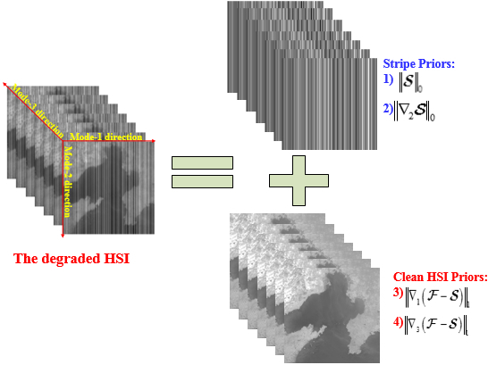
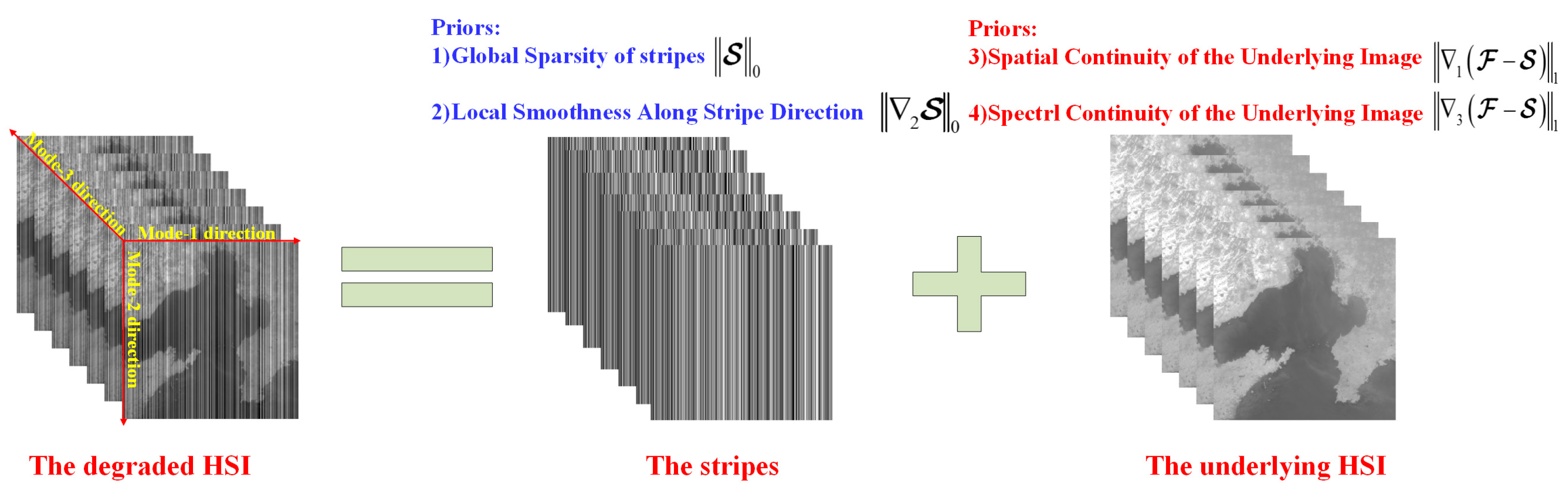
Considering the characteristic of stripes, sparse representation and sparsity promoting priors have been utilized to remove the stripes in HSIs [15,16,32,33]. However, this sparsity characteristic has not been considered under a tensor framework. In this paper, the tensor-based non-convex sparse model utilizes the sparse priors to estimate stripes from the observed images, using two sparse priors and two sparse priors. One sparse prior is related to the global sparse distributional property of stripes, and the other is related to the directional property of stripes (along the gradient stripes). One sparse prior characterizes the continuity of image (across-stripe direction), and the other denotes the correlation along the spectral dimension. Section 3.2 further explains the reasons for choosing these priors. Figure 1 shows the framework and priors of the proposed method. The ∇1 and ∇2 represent unidirectional TV operators of the along-stripe direction and the perpendicular direction, respectively, and ∇3 represents the difference operator along the spectral direction. To solve the proposed GLTSA, we extended the proximal alternating direction method of multipliers (PADMM)-based algorithm [16] to the tensor framework.
The main contributions of the proposed HSI destriping methods are as follows:
- (1)
- We transformed an HSI destriping model to tensor framework, to better exploit high correlation between adjacent bands. In the tensor framework, a non-convex optimization model was constructed to estimate the stripes and underlying stripe-free image simultaneously for higher spectral fidelity.
- (2)
- The proposed method fully considers the discriminative prior of the stripes and the stripe-free image in tensor framework. We represent and analyze intrinsic characteristics of the stripes and stripe-free images, using and , respectively. Experiment results show that the proposed method outperforms existing state-of-the-art methods, especially when the stripes are non-periodic.
- (3)
- We used the PADMM to solve a non-convex optimization model effectively. Extensive experiments were conducted on simulated data and real-world data. The proposed scheme achieved superior performance in both quantitative evaluation and visual comparison compared with existing approaches.
The remainder of this paper is organized as follows. Section 2 gives some preliminary knowledge on the tensor notations and intrinsic statistical characteristics of stripe and stripe-free images. Section 3 presents the formulation of our model, along with a PADMM solver. In Section 4, we discuss the experiments and analyze the selection of parameters. Section 5 concludes this paper.
2. Intrinsic Statistical Property Analysis of Stripe and Clean Images
2.1. Notations and Preliminaries
In this paper, we use boldface Euler script letters (e.g., ), boldface capital letters (e.g., X), boldface lowercase letters (e.g., x), and lowercase letters (e.g., ), to denote tensors, matrices, vectors, and scalars, respectively. For an N-order tensor, , its element at location () is denoted as . The norm of tensor is defined as and -norm is defined as the number of non-zero elements in . The inner product and Hadamard product of two N-order tensors, , are defined as and , where and . For more information about tensor algebra, please refer to [37].
2.2. Priors and Regularizers
This subsection analyzes the priors of stripes and stripe-free image and design appropriate regularizers to describe the priors in a destriping model.
2.2.1. Global Sparsity of Stripes
When the stripes are few in an HSI image, the stripes are regarded as a sparse tensor [16]. Naturally we choose -norm, the number of nonzero elements, to measure the sparsity of stripe component :
Based on the sparsity constraint, the stripes are simply separated, while keeping useful information. However, when the stripes are extremely dense, it is difficult to restore HSIs. Heavy stripes, which means that the percentage of stripes in an image is high (usually more than 50%), significantly damage reliable spatial and spectral information. A single -sparsity measurement for stripes can no longer depict reasonably intrinsic characteristics of stripes. Thus, it is necessary to explore other regularizers for stripes and HSIs to deal with heavy stripes.
2.2.2. Local Smoothness along Stripe Direction
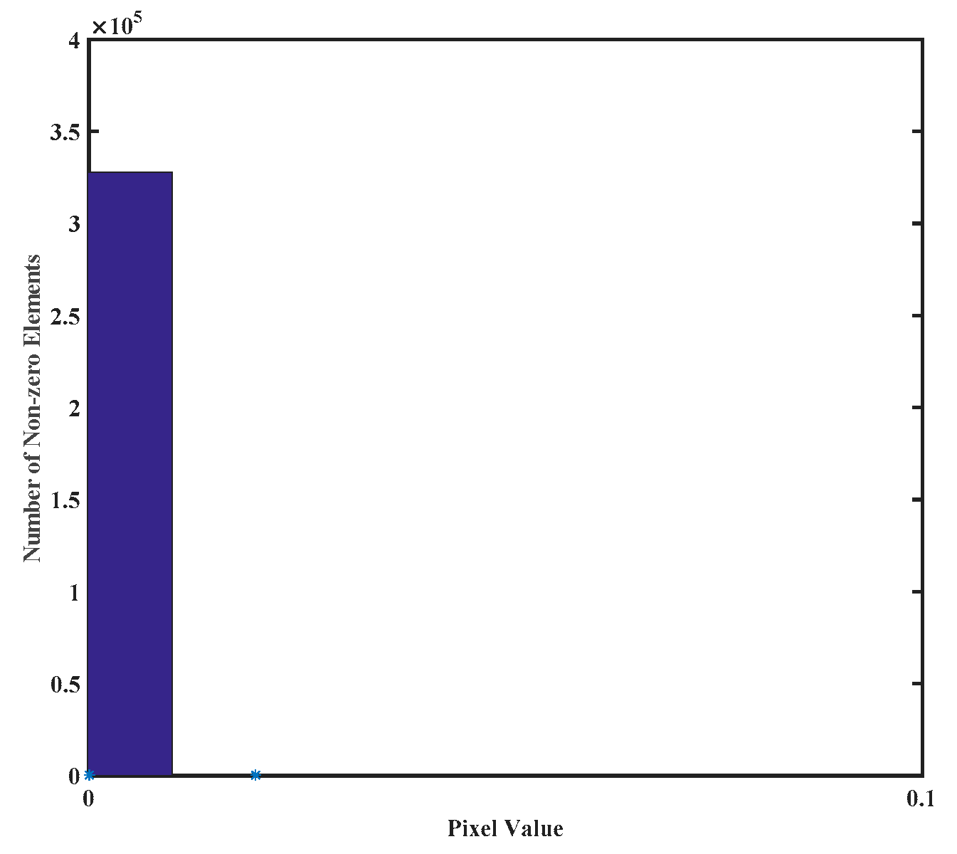
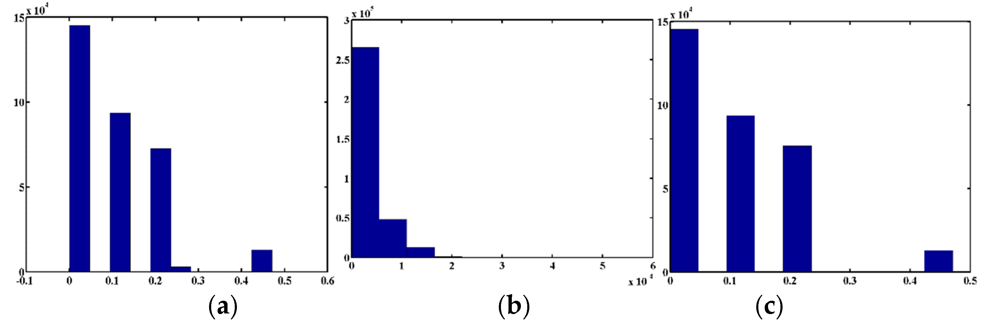
Besides the global sparsity of stripes mentioned above, more powerful sparsity is embodied in gradient domain along stripe. Figure 2 represents statistical distribution of non-zero elements in , where is the gradient operator along the stripe, and the stripe in Figure 2 is extracted from the promising method proposed in [13]. Most gradient along the stripes are so small that they are close to zero. The sparsity in gradient domain essentially reflects local smoothness along stripe direction. The local sparsity measurement for stripes is as follows:
2.2.3. Continuity of HSIs along Spatial Domain
As suggested in [16], for an HSI , the spatial information long mode-1 (or spatial horizontal direction) is continuous. From Figure 3b, the stripes severely destroy the local spatial continuity in mode-1, indicating that the horizontal gradient of should be as small as possible, to keep the continuity. With this observation, the -norm regularization on the gradient of below is used to describe the local continuity of the image in the spatial domain:
where represents horizontal gradient of .
2.2.4. Continuity of HSIs along Spectral Domain
Figure 4 represents histograms of spectral gradient of degraded HSIs, the stripe-free image, and the stripes of WDCM in Figure 3. The spectral gradient histogram (Figure 4b) of the stripe-free HSI includes more zeroes and smaller values than that of the stripes (Figure 4c), which illustrates that the underlying HSI possesses strong continuity along the spectral direction. The low-rank prior of stripes will be violated for real HSI, especially when the stripes are fragments [34]. It is natural to minimize the norm of the spectral gradient of :
3. The GLTSA Destriping Method
3.1. Stripe-Degraded Model
The stripes in HSI can be classified into two categories from the mechanism of noise generation, including additive stripes [14] and multiplicative stripes [38]. The multiplicative stripes can be transformed to additive stripes by logarithmic transformation [39]. Thus, the observation model of stripe-degraded HSI is formulated as F = U + S [13,14], and the corresponding tensor-based reformulation is as follows:
where , and indicate the degraded image, the unknown clean image, and stripes, respectively. Moreover, h and v indicate the horizontal and vertical pixel numbers in spatial domain, and b represents the number of spectral bands.
3.2. The GLTSA Destriping Model
Based on the discussion for the priors for both the image and stripe components in Section 2.2, the regularizers in the proposed model can be formulated as follows:
where are weighted parameters. To tackle this double-objective non-convex optimization problem, we can transform it to the following single-objective non-convex optimization problem with constraint :
Note that the optimization problem in Equation (7) substantially differs from the models proposed in [13,16]. The main difference is that the two models are matrix-based, while our method is tensor-based. The two models in [13,16] have not considered the spectral correlation, which would result in spectral distortion. The proposed method introduces the spectral prior to avoid this issue.
3.3. Optimization Procedure and Algorithm
There are two non-convex regularization terms in Equation (7). In order to handle them, we first present Lemma 1, the non-convex optimization problem can be converted into convex optimization with this Lemma. Then the PADMM method is utilized to solve it, and theoretically guarantee the convergence at the same time.
Lemma 1.
(Mathematical Program with Equilibrium Constraints (MPEC) equation [39]). For any given vector , the following holds:
where < > represents the inner product of two vectors, and denotes the element-wise product. The absolute of w stands for the absolute value of each element of w. Then, is the unique optimal solution of the minimization problem in Equation (8), and .
Lemma 1 can be intuitively extended to the tensor version, i.e., Lemma 2:
Lemma 2.
For any given tensor , the following holds:
where is the unique optimal solution of the minimization problem in Equation (9).
Proof.
Similar to Lemma 1, see details in [39]. ☐
According to Lemma 2, the objective function (7) can be reformulated as follows:
According to ADMM optimization framework, we introduce four auxiliary variables and , and then equally transform Equation (10) as follows:
The augmented Lagrangian form of (11) is as follows:
where the s are positive scalar parameters and the s (i = 1,2,3,4,5) are the scaled Lagrange multipliers.
1. subproblem: This subproblem can be written as follows.
It has a close-form solution [16]:
where , is the unit tensor of the same size as .
2. subproblem: This subproblem is a non-convex optimization problem.
According to [40,41], the can be updated as follows:
where is a hard-thresholding function, and is a given positive threshold.
3. subproblem: This subproblem is a quadratic minimization problem.
Based on 3D fast Fourier transform (FFT), the explicit close-form solution is as follows:
where , , fft denotes 3-D FFT, ifft is inverse 3-D FFT.
4. subproblem: By Lemma 2, the subproblem of is
which is equivalent to the following:
Based on the constraint , it still has a closed-form solution:
where .
5. subproblem: when other variables are fixed, variable can be updated by
By using soft-threshold shrinkage operator [42], the solution is given by the following equation:
where .
6. subproblem: Similar to optimization for variable , can be updated by the following equation:
The closed-form solution is given by the following equation:
7. Multiplier subproblems: The update form of Lagrange multipliers s (i = 1, 2, 3, 4, 5) are as follows:
All the subproblems have the closed-form solutions, which guarantee the accuracy of the model. The GLTSA destriping algorithm is summarized in the following Algorithm 1. With regard to computational complexity, for an HSI with dimensions of h×b×v, the time complexity of GLTSA is proportional to O(hbv·log(hbv)).
| Algorithm 1. The GLTSA destriping algorithm |
| Input: The observed degraded image with stripe , parameters , the maximum number of iterations Nmax=103, and the calculation accuracy tol = 10−4. |
| Output: The stripes |
| Initialize: (1) k=0, ; While and k < Nmax do; (2) Update by Equation (14); (3) Update by Equation (16); (4) Update using 3-D FFT by Equation (18); (5) Update by Equation (21); (6) Update by Equation (23); (7) Update by Equation (25); (8) Update the multipliers , i = 1, 2, 3, 4, 5 by Equations (26)–(30). End While |
4. Experiment Results
To verify the effectiveness of GLTSA on simulated and real data, we compared with six state-of-the-art methods. The first four methods belong to band-by-band restoration matrix-based methods, including the unidirectional total variation model (UTV) [14], Directional L0 Sparse (DL0S) Model [16], the wavelet Fourier adaptive filter (WFAF) [22], and statistical gain estimation (SGE) [23]. The other three methods are tensor-based or tensor-like-based methods, including anisotropic spectral–spatial TV (ASSTV) model [19], Low-Rank Tensor Decomposition (LRTD) [20] model, and Low-Rank Multispectral Image Decomposition (LRMID) model [34]. The codes of WFAF, UTV, ASSTV, and LRMID can be downloaded from the website (http://www.escience.cn/people/changyi/codes.html). The code of DL0S can be downloaded from the website (http://www.escience.cn/people/dengliangjian/codes.html). The code of LRTD is available on the website (https://www.researchgate.net/profile/Yong_Chen96). In the simulated experiments, we add periodic and non-periodic stripes, as suggested in [34]. Before this, it is necessary to determine two indicators of the stripes: (1) the intensity represents the stripes’ absolute mean value (denoted by I) and (2) the ratio (or percentage) of the stripe area to the whole image (denoted by r). We selected several typical combinations of I and r in the simulated experiments, that is I ∈ {20,50,100}, r∈{0.2,0.4,0.6,0.8, 0 - 1 }, where r = 0 − 1 indicates that the percentage of stripes varies from band to band. The test data are normalized to a range of 0 to 1. In the following experiments, we manually tuned the parameters. For the experiments, we used MATLAB (R2016a) on a desktop with 8Gb RAM and Inter(R) Core(TM) CPU i5-4590: @3.30 GHz.
4.1. Simulated Data Experiments
In the simulated experiments, we generated periodic stripes and non-periodic stripes under different intensities and ratios. We used the Hyperspectral Digital Imagery Collection Experiment (HYDICE) image dataset of the Washington DC Mall (WDCM in short) as the ground truth image, which is available on website (https://engineering.purdue.edu/biehl/MultiSpec/hyperspectral.html). There are 191 spectral bands, and its spatial resolution is 1208 × 307 pixels. Because the original image is too large, which is very expensive in terms of computational cost, a sub-image of size 256 × 256 × 10 is extracted for the simulated experiment.
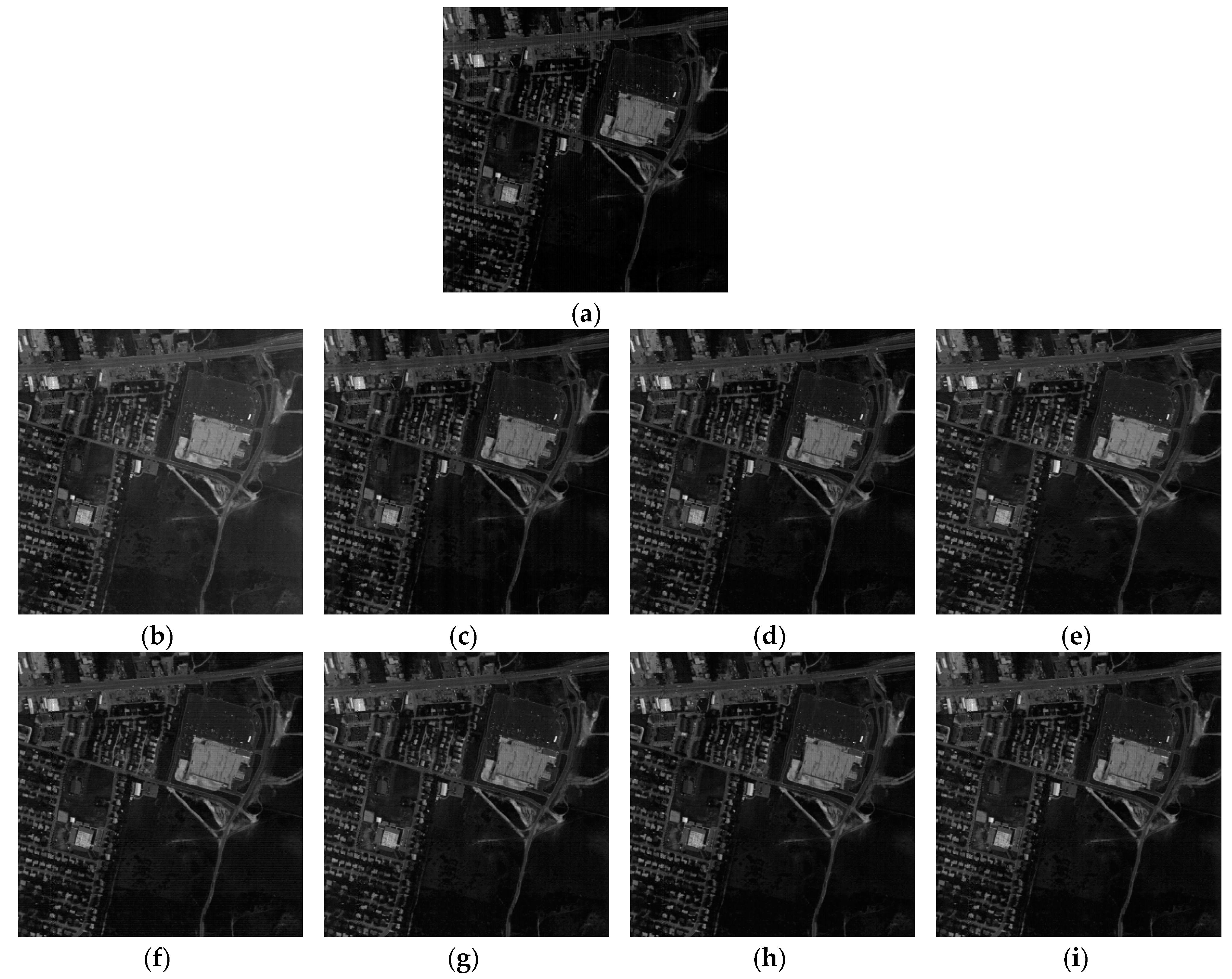
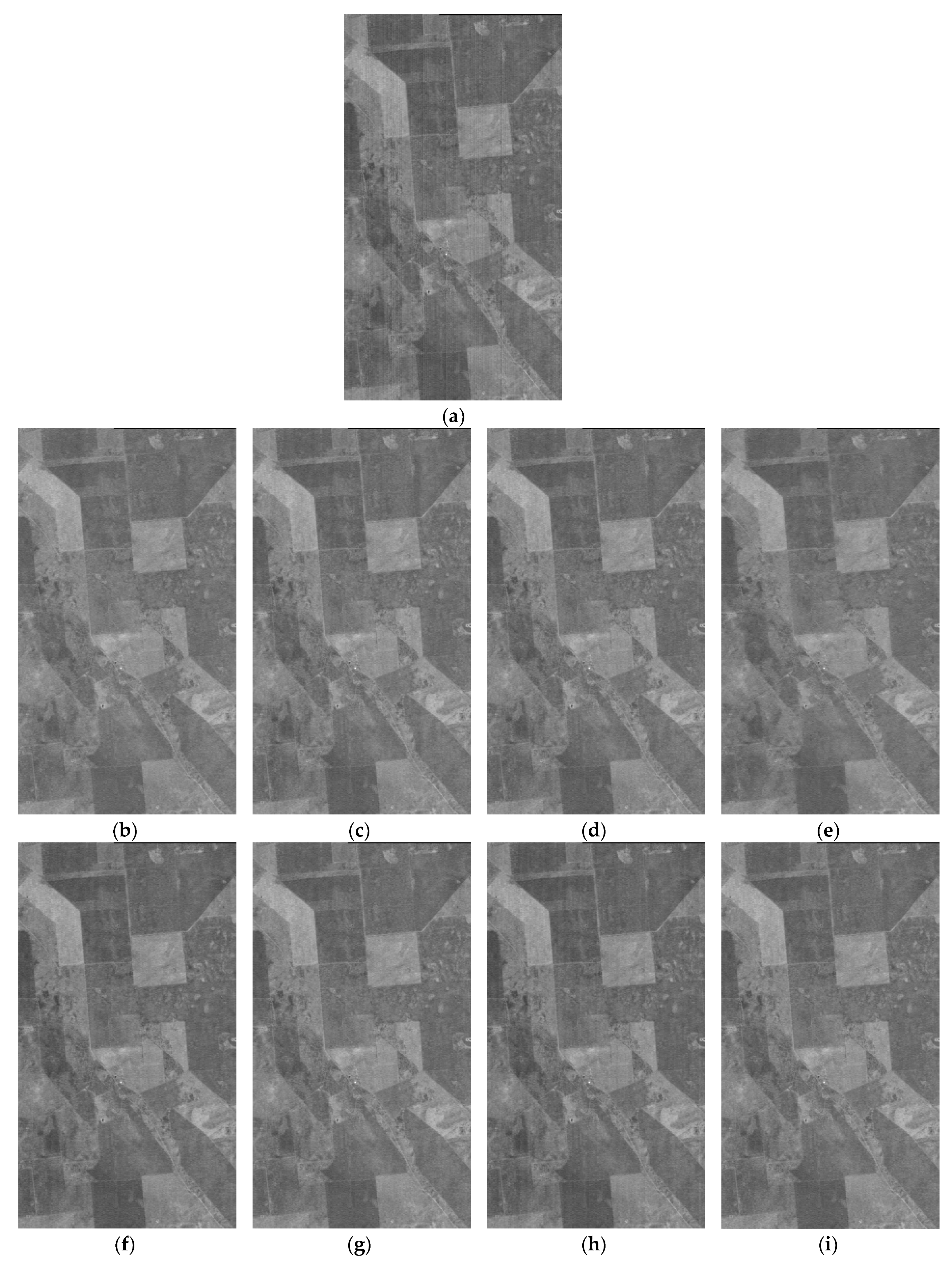
(a) Visual effect comparison: To evaluate the destriping effectiveness of GLTSA, we simulated many degraded cases. We selected one representative band of WDCM to show the destriping results. The original images are presented in Figure 5a and Figure 6a, and the images are degraded by periodic stripes (I = 60, r = 0.8) and non-periodic stripes (I = 60, r = 0.4) are listed in Figure 5b and Figure 6b, respectively. The destriping results obtained by different methods are illustrated in Figure 5c–j and Figure 6c–j, where significant differences in visual quality can be observed.
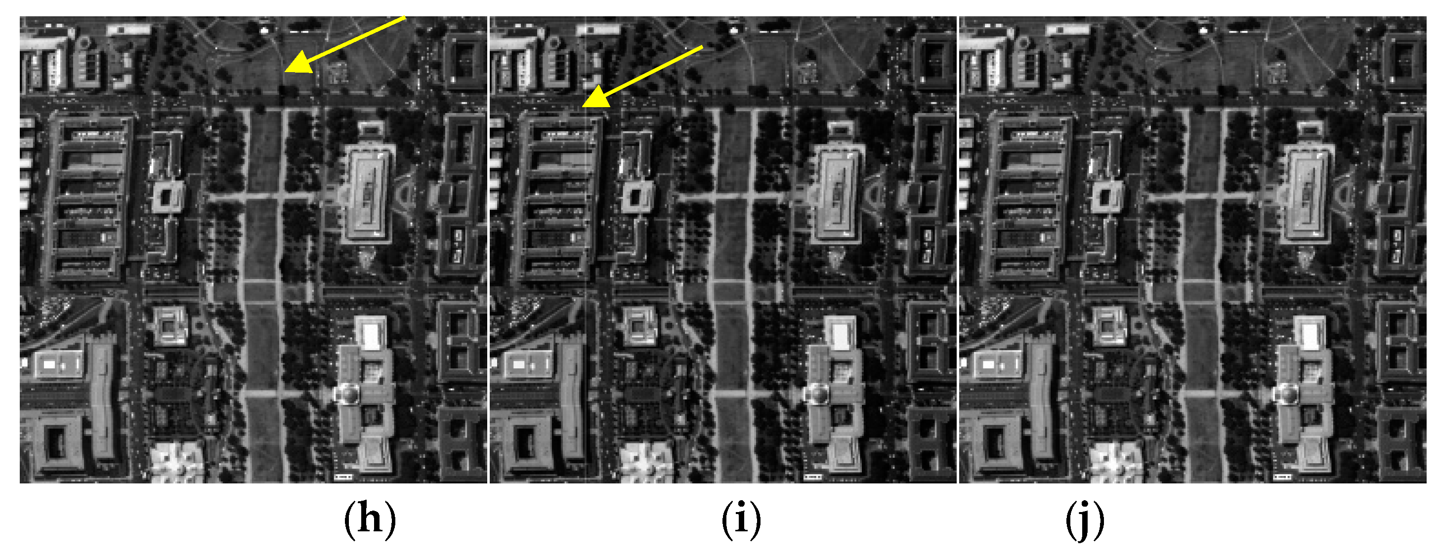
When the intensity and ratio are low, most of the comparative methods obtain similar visual quality comparable to the proposed method. But when the intensity and ratio are high, most of the comparative methods have poor results, in both cases of the periodic and non-periodic stripes. For example, the result images are distorted, blurred, and over-smoothed in Figure 5c–e. LRTD has obtained satisfactory results due to that it directly processes the data cubes instead of a band-by-band process. There are almost no obvious residual stripes in DL0S, LRMID, and LRTD. Even though the LRMID, DL0S, and LRTD achieve similar visual quality as the proposed method, there are still residual stripes in the images from the enlarged part (yellow box), especially in the non-periodic stripes case (see Figure 6g–i). The results show that GLTSA can effectively remove stripes and retain more details and structure.
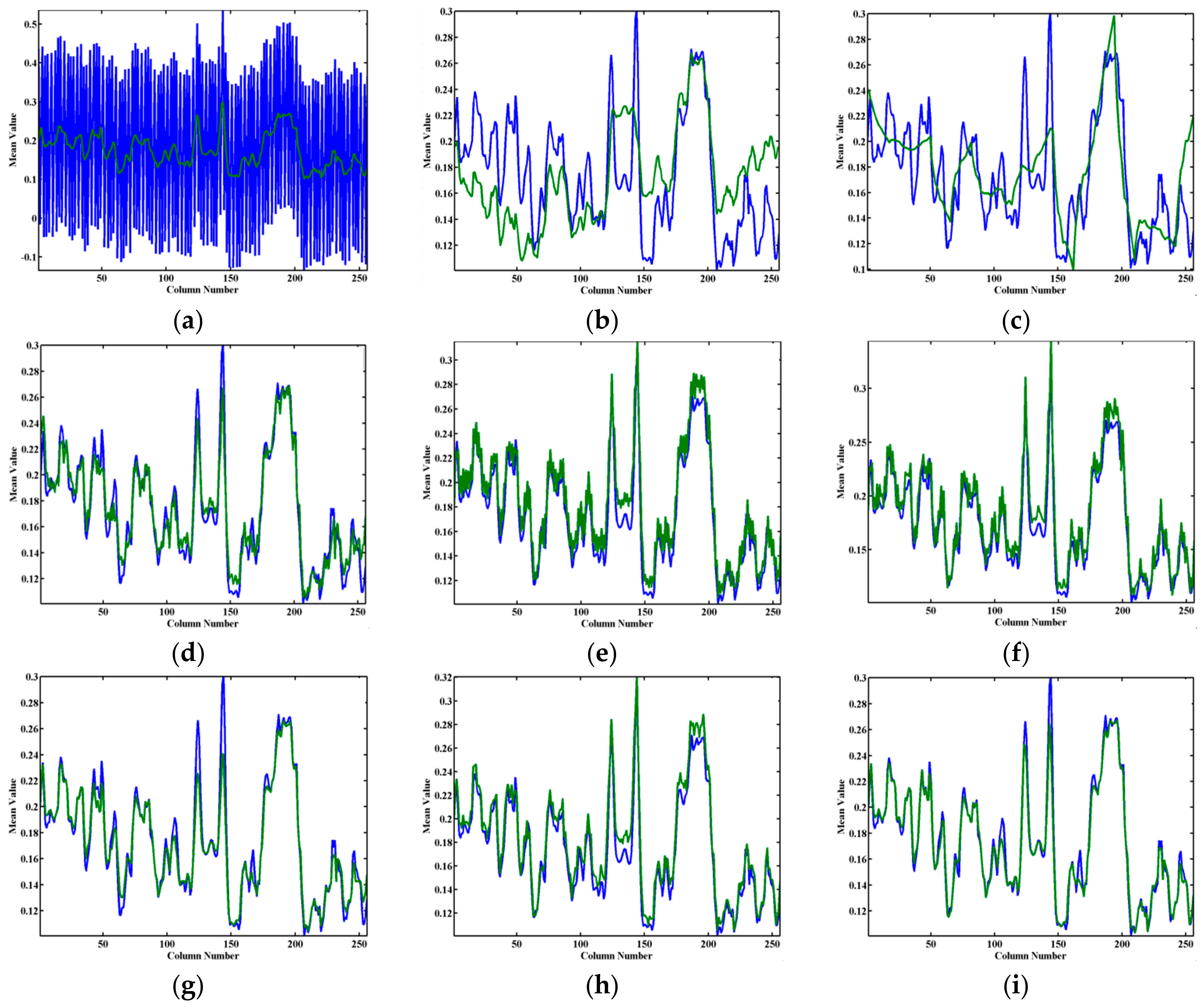
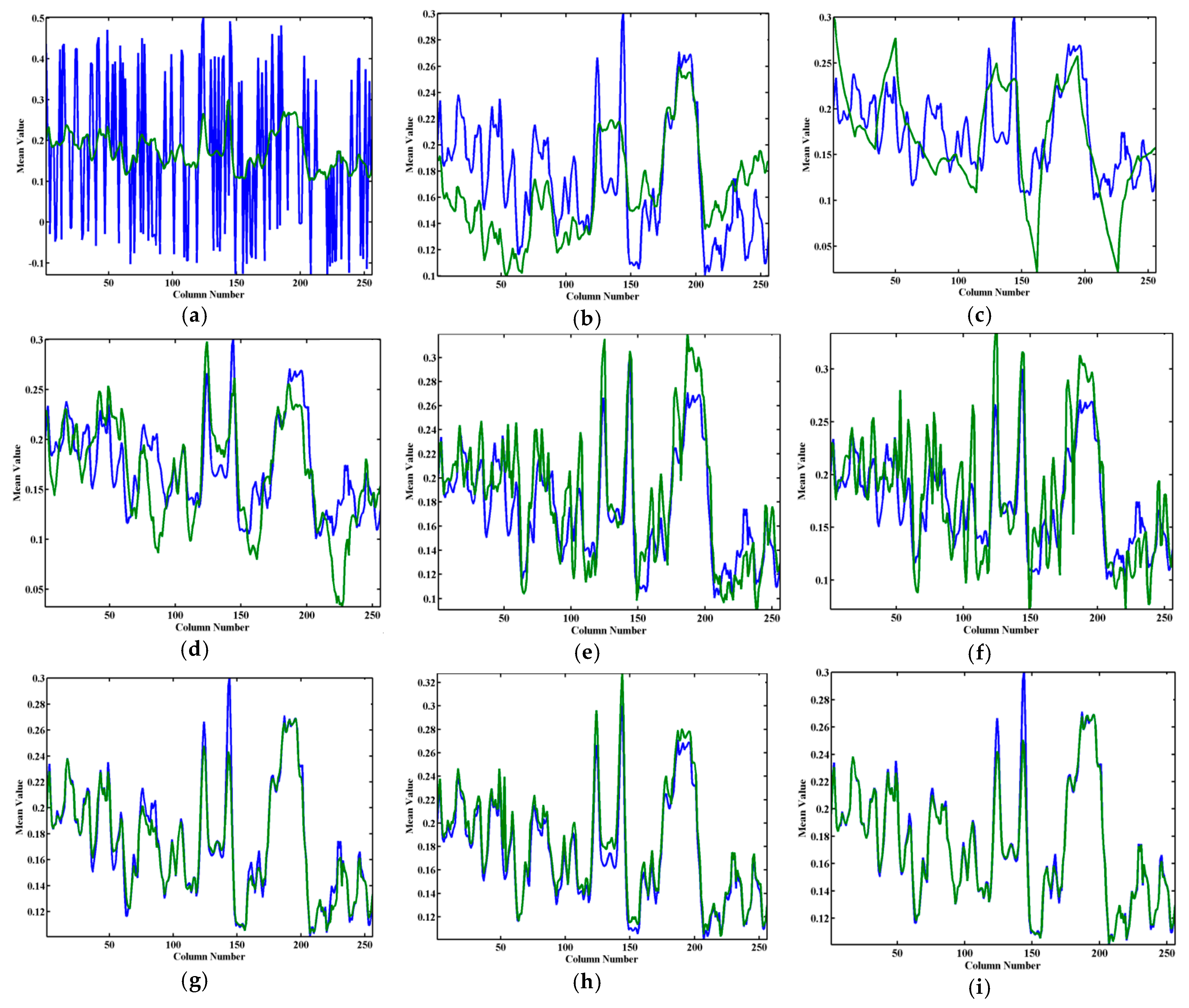
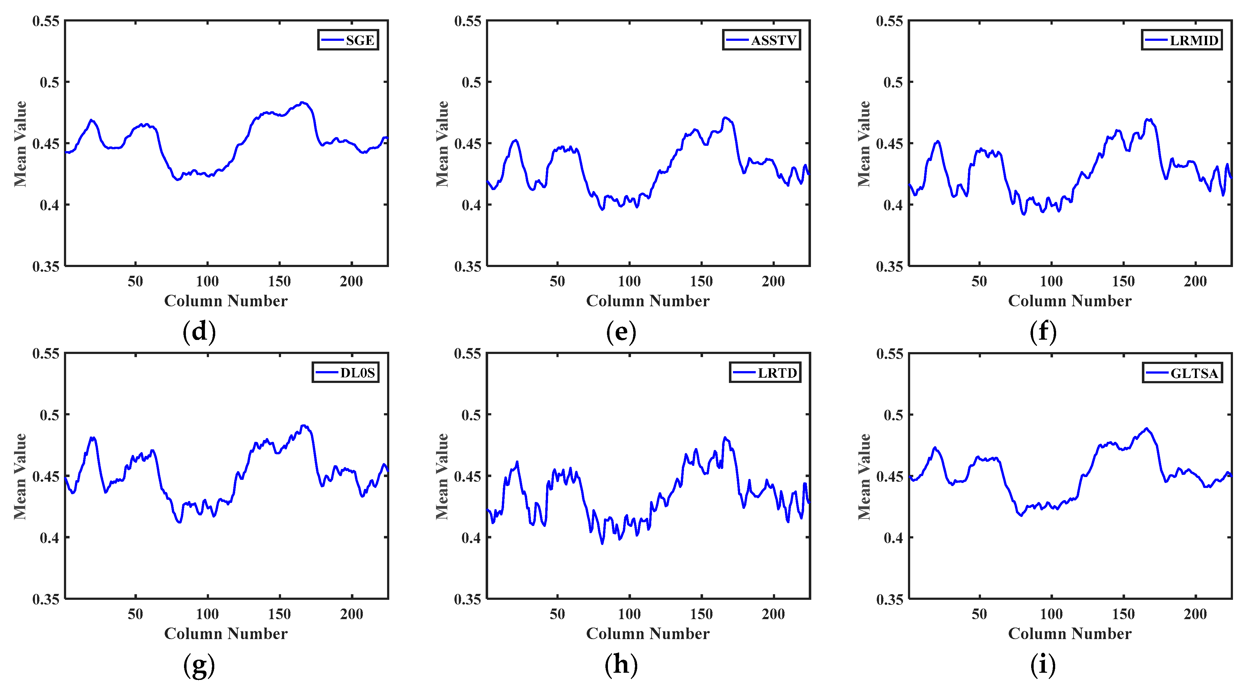
(b) Qualitative Assessment: For the evaluation of GLTSA, we adopt the mean cross-track profile (MCTP) to compare the performance. The curves in Figure 7 and Figure 8 represent the MCTPs of Figure 5 and Figure 6, respectively. The horizontal axis indicates the column number, while the vertical axis denotes the mean digital number value of each column. The existence of stripes results in rapid fluctuations (blue curve) in Figure 7a; the stripes are more or less suppressed by the eight methods as shown in Figure 7b–i. From Figure 7b–d, we can see that UTV, WFAF, and SGE methods fail to restore original MCTP (green curve). There are still fluctuations in Figure 7e,f. This indicates that the images estimated by these methods are distorted or blurred. Although the profiles produced by DL0S and LRTD are better than other methods, the MCTP of GLTSA is closer to the original, showing no difference with the results listed in Figure 5. A similar case is shown in Figure 8.
(c) Quantitative comparison: To verify the robustness of GLTSA under different noise levels, we adopted five acknowledged quantitative indices, namely the mean peak signal-to-noise ratio (MPSNR) [43], mean structural similarity (MSSIM) [43], feature similarity (MFSIM) [44], mean spectral angle mapper (SAM) [45], and erreur relative globale adimensionnelle de synthese (ERGAS, relative dimensionless global error in synthesis, in English) [46]. The definitions of these indexes are as follows:
where b represents the number of spectral bands, and are the restored image and the original clean image of i-th band (they are of the same size), and ni represents the total number of pixels of image of .
where and represent the average value of x and y images; and stand for the variance of x and y images; and is the covariance of these two images. C1 and C2 are constant here.
where Ω means the whole image spatial domain, is the similarity of images f1 and f2 at each location , and is the weight of in the overall similarity between images f1 and f2.
where S1 = (x1, x2, . . . , xn) and S2 = (y1, y2, . . . , yn) represent the spectral vectors at the same location in HSI.
where h, v, and b are defined above. RMSE(xi) denotes the root-mean-square error (RMSE) for image xi, and μ(i) denotes the mean of image yi.
The MPSNR and MSSIM are used to measure the performance of spatial information, while the global performance of spectral distortion is evaluated by SAM and ERGAS. The larger the MPSNR and MSSIM values, the smaller the SAM and ERGAS values, and both are indicating that the effect of destriping is better. Table 1 and Table 2 list the quantitative indices of all the destriping methods with simulated periodic and non-periodic stripes, respectively. The boldface digits in Table 1 and Table 2 represent the best results. GLTSA outperforms LRTD, DL0S in these indices except only a few cases. As the intensity and ratio of stripes increases, the values of MPSNR and MSSIM decrease, while the GLTSA shows stable results, indicating robustness. The SAM and ERGAS values of GLTSA are the smallest among all compared methods; this indicates that the spectral distortion of GLTSA is the lowest. The quantitative evaluation results are in line with the visual effects.
4.2. Experiments on Real Data
In this experiment, we choose two real image datasets. The first one is Urban data from Hyperspectral Digital Imagery Collection Experiment (HYDICE). Some bands are degraded with non-periodic stripes. The original size is 307 × 307 × 210, and a sub-image with the dimensions 307 × 307 × 8 (from band 1 to band 8) is extracted for the experiment. The original data are available on the website (http://www.erdc.usace.army.mil/). The second data are collected by EO-1 Hyperion L1R-level sensor. These data were captured in Australia on December 4, 2010. The size of original image is 3858 × 256 × 242, and a sub-image of 400 × 225 × 10 (from band 54 to band 63) is used in our experiment, which is available online (http://remote-sensing.nci.org.au/). The data are normalized to [0,1] before processing.
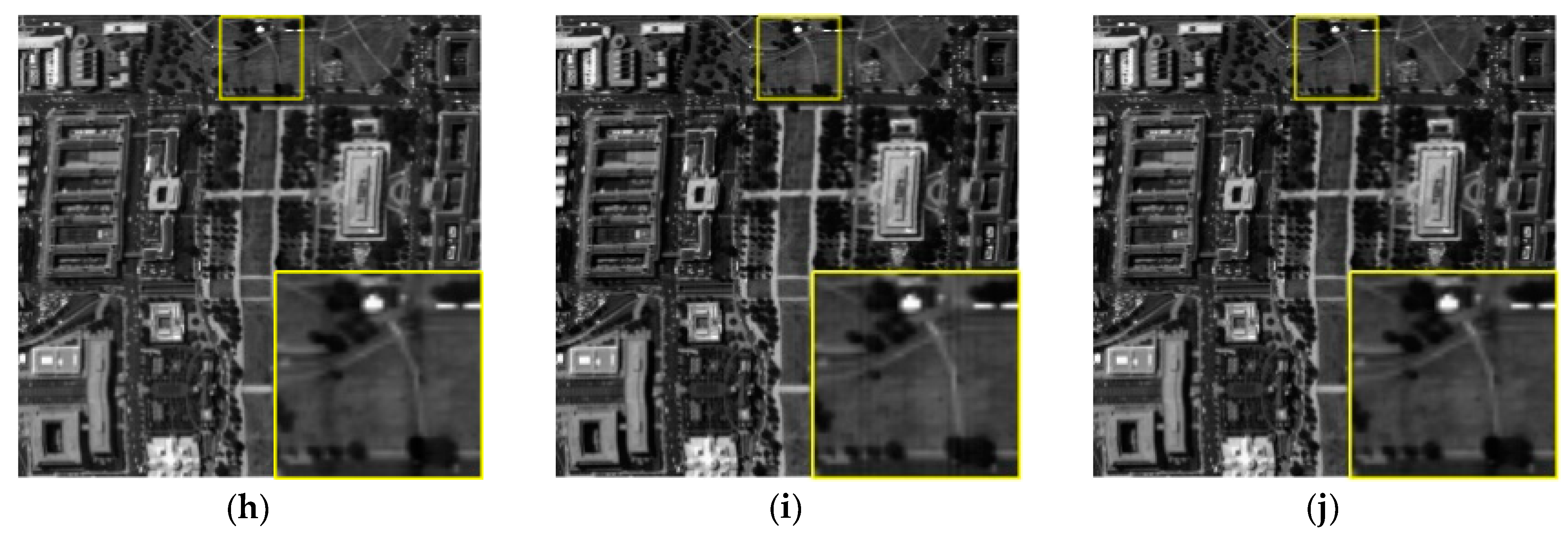
The results of all the methods on the two real data are displayed in Figure 9 and Figure 10. From Figure 9b–d and Figure 10b–d, UTV, WFAF, and SGE result in the distortion of details and structure. Erroneous horizontal stripes are introduced by ASSTV, LRMID, and LRTD, as shown in Figure 9e–h and Figure 10e–h. DL0S can eliminate most of the stripes, but still leave some obvious stripes, as shown in Figure 9h and Figure 10h. Regardless of the level of image quality, GLTSA is able to remove the stripes effectively, while retaining the details.
The MCTPs of Figure 9 and Figure 10 are shown in Figure 11 and Figure 12, respectively. The MCTP of the Urban data is shown in Figure 11a, while Figure 11b–i shows the MCTPs of the compared methods. The profiles of LRMID and LRTD have obvious fluctuations, which indicate residual stripes, and the profiles of WFAF and UTV show over-smoothing, which suggests details are lost. Figure 11i indicates that GLTSA can realize the desired result, while keeping more details.
Since there is a lack of ground-truth images as reference data, we adopt two non-reference destriping indices, including the inverse coefficient of variation (ICV) [38] and mean relative deviation (MRD) [38]. The definitions of these two indices are introduced in [38]:
where Rm and Rs represent the mean and standard deviation of pixel values in the same region of the destriping and original images, respectively; and xi and yi are the pixel values in the destriping and original images, respectively.
Table 3 lists the results of two non-reference indices. The best results are given in bold. The GLTSA outperforms the compared methods in most cases. The best results of compared methods have only little difference with ours. The GLTSA outperforms on destriping the state-of-the-art methods for comparison.
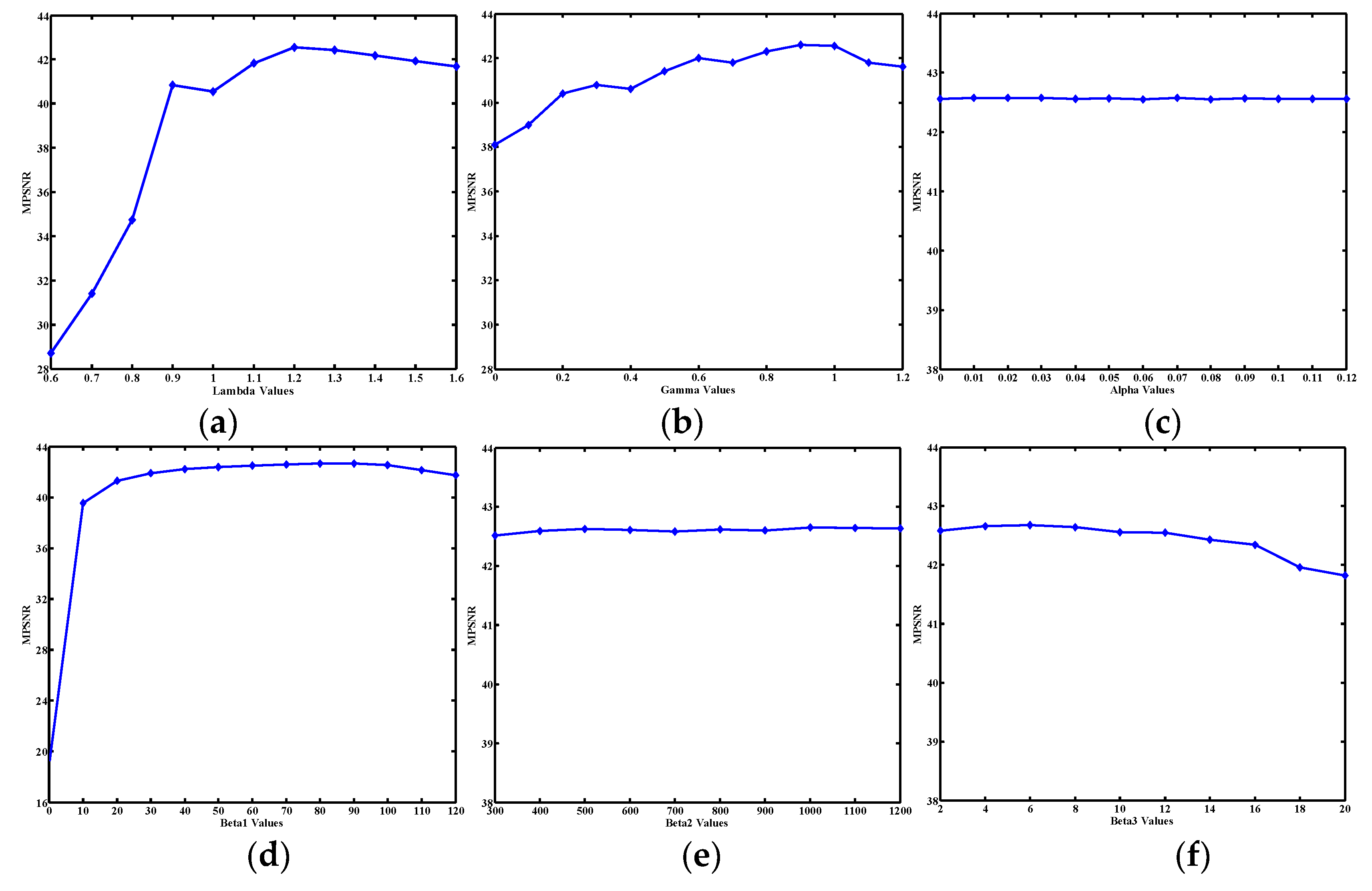
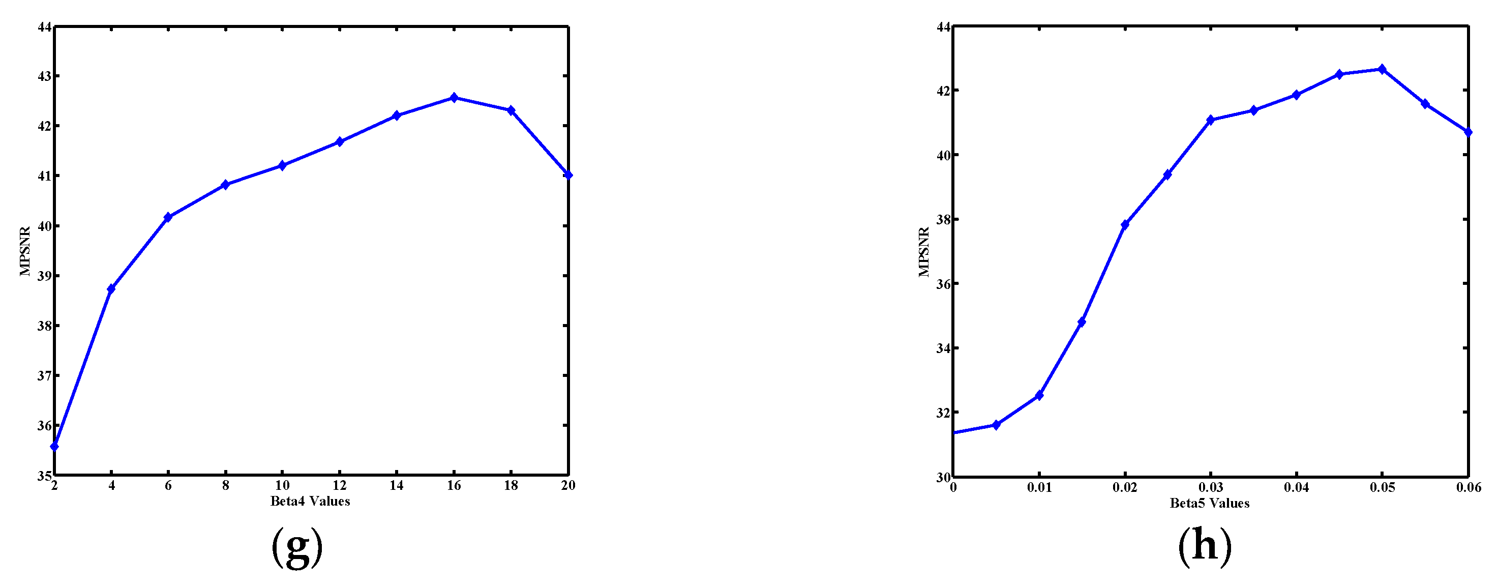
4.3. Analysis for Parameter Settings
At present, the selection of regularization parameters automatically or adaptively of different sensors is still a difficulty for many algorithms, which will be further researched in our future work. In this paper, the distributional properties of sparsity, smoothness, and spatial–spectral continuity are constructed as constraint terms to estimate the stripe component. Our model contains eight regularization parameters (12): and (i = 1, 2, 3, 4, 5). Since the noise intensity and proportion of stripes have many different combinations, we tuned them empirically to obtain a more accurate estimation. To find the appropriate parameter values, we chose the mean PSNR (MPSNR) as the selection criterion to evaluate and analyze the effect. We conducted experiments on different simulated data. To show the influence of parameter tuning, we used the WDCM dataset as an example. It is obvious that the optimal values of eight parameters are in the eight-dimensional parameter space, but it will be time-consuming. To mitigate this problem, we adopt a greedy algorithm to determine the optimal value of parameters in turn. Experiment results show that, although the parameters obtained by this method are not globally optimum, the destriping results are still excellent.
The function curve of MPSNR values and the regularization parameters, , is plotted in Figure 13a; the results show that, when λ increases from 0.6 to 1.2, the MPSNR is obviously improved, and then the MPSNR reduces slightly when is further increased. That is to say, the highest MPSNR value of is reached near 1.2. The function curve of MPSNR values with parameter is listed in Figure 13b. With the increase of , the highest MPSNR value is reached near 1. It shows similar trends as . Since there are many degradation scenarios in our implementation, the parameters are not fixed; they are varied in the [1.1, 1.3] range for and [0.8, 1] for . The relationship between MPSNR and the parameter is depicted in Figure 13c. It is observed that MPSNR does not change much with the change of . This means that the GLTSA is robust with . In fact, the image with severe stripes will prefer a larger but a lower . The value of is fixed within the range of [10–5, 10–4].
The relationship between MPSNR and the parameters are listed in Figure 13d–h, respectively. From Figure 13d, it is observed that MPSNR changes very little with parameter in the range of [20,100]. Similar to the analysis of parameter , it can be seen from Figure 13e,f that our method is robust with and . It can be seen from the Figure 13g,h that the GLTSA obtains the best result when . Based on the above evaluation results, the parameter values in this paper are empirically set as .
4.4. Convergence Analysis and Comparison of Running Time
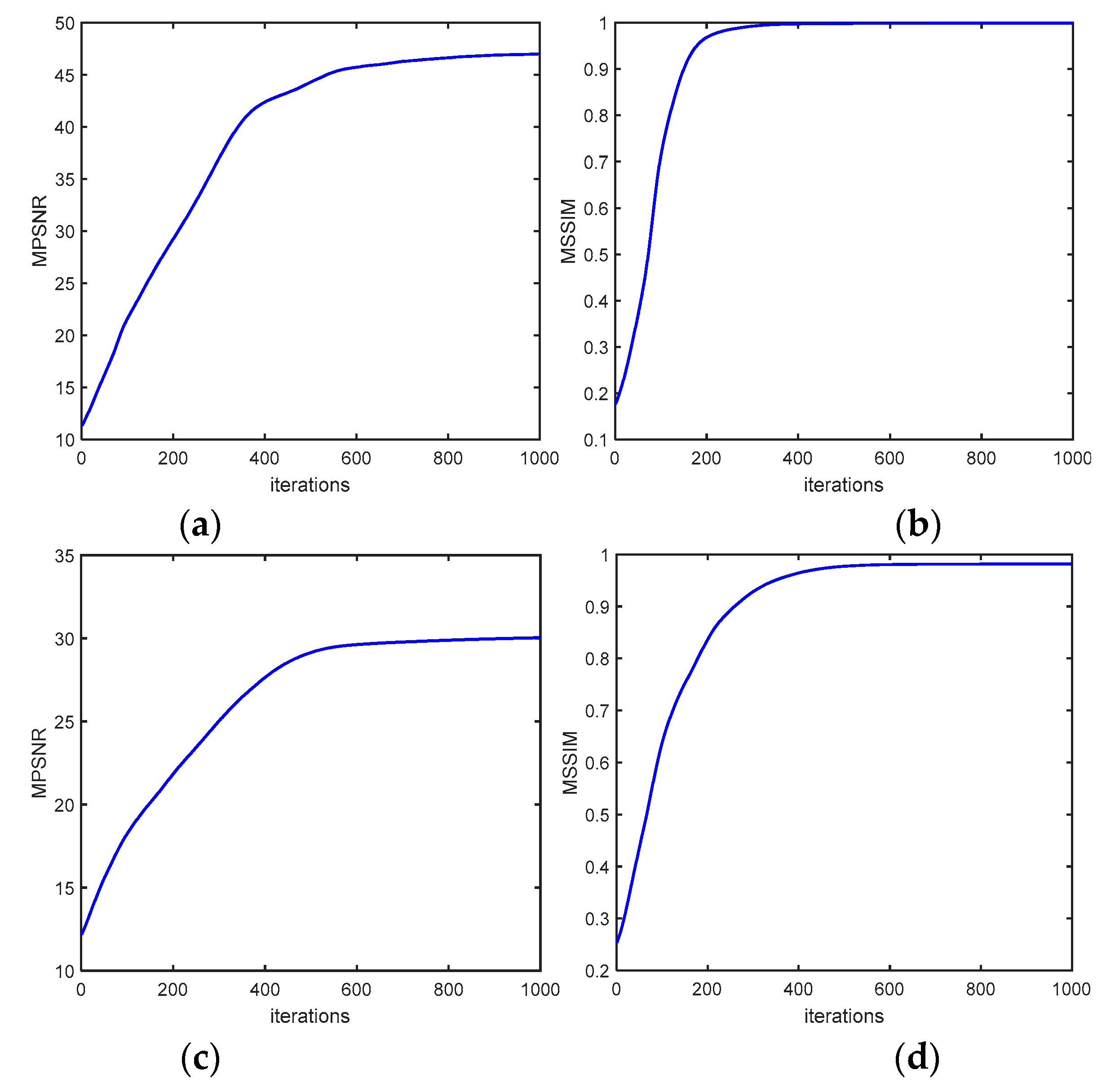
Figure 14 shows the relationship between the MPSNR and MSSIM values and the number of iterations of the GLTSA solver. Figure 14a,b is the periodic situations with (r = 0.5, I = 100), Figure 14c,d is the non-periodic situations with (r = 0.9, I = 60). As the iterations go on, GLTSA converges as relative changes of MPSNR and MSSIM converge to zero.
For time complexity, we show the running times of all the methods in Table 4. It is easy to see that, for 10 bands of WDCM data, the running speeds of methods UTV, WFAF, and SGE are obviously faster than other methods. However, according to the visual effect (Figure 5 and Figure 6) and index analysis (Table 1 and Table 2), their results are worse. In fact, it is hard to find the best trade-off between good results and time complexity. Compared with other methods, the running speed of our method is not the fastest, but our results are the best.
5. Conclusions
This paper presents a tensor sparse approximation model for HSI destriping. The characteristics of image and stripe are simultaneously modeled under tensor-based sparse approximation framework. More specially, the -norm of stripes and its gradient are used to characterize the global sparsity of the stripes and local smoothness along stripes direction. The -norm of the gradients of underlying images in spatial and spectral are utilized to depict the continuity. The tensor-based PADMM algorithm is adopted to handle the non-convex tensor optimization model. Experiment results have demonstrated that GLTSA has better striping performance and lower spectral distortion compared with the existing methods.
Author Contributions
X.K. conducted experiments, analyzed the results, and wrote the paper; Y.Z. conceived the experiments and is responsible for the research analysis; J.C.-W.C., and S.G.K. checked the language and grammar, J.X. collected and processed the original data. All co-authors helped revise the manuscript. All authors have read and agree to the published version of the manuscript.
Funding
This work was supported by the National Natural Science Foundation of China (61771391, 61371152), the Shenzhen Municipal Science and Technology Innovation Committee (JCYJ20170815162956949, JCYJ20180306171146740), the National Research Foundation of Korea (2016R1D1A1B01008522), the Innovation Foundation for Doctor Dissertation of Northwestern Polytechnical University (CX201917), and the natural science basic research plan in Shaanxi Province of China (No. 2018JM6056). We are grateful to the authors of the compared methods for providing the source codes.
Conflicts of Interest
The authors declare no conflict of interest.
References
- Xue, J.; Zhao, Y.; Liao, W.; Chan, J.C.-W. Nonlocal Low-Rank Regularized Tensor Decomposition for Hyperspectral Image Denoising. IEEE Trans. Geosci. Remote Sens. 2019, 57, 5174–5189. [Google Scholar] [CrossRef]
- Sánchez, N.; González-Zamora, Á.; Martínez-Fernández, J. Integrated hyperspectral approach to global agricultural drought monitoring. Agric. For. Meteorol. 2018, 259, 141–153. [Google Scholar] [CrossRef]
- Chen, J.; Shao, Y.; Guo, H. Destriping CMODIS data by power filtering. IEEE Trans. Geosci. Remote Sens. 2003, 41, 2119–2124. [Google Scholar] [CrossRef]
- Yi, C.; Zhao, Y.Q.; Yang, J. Joint Hyperspectral Superresolution and Unmixing With Interactive Feedback. IEEE Trans. Geosci. Remote Sens. 2017, 55, 3823–3834. [Google Scholar] [CrossRef]
- Yang, J.; Zhao, Y.Q.; Chan, C.W. Coupled Sparse Denoising and Unmixing With Low-Rank Constraint for Hyperspectral Image. IEEE Trans. Geosci. Remote Sens. 2015, 1–16. [Google Scholar] [CrossRef]
- Yi, C.; Zhao, Y.Q.; Chan, J.C.W. Spectral super-resolution for multispectral image based on spectral improvement strategy and spatial preservation strategy. IEEE Trans. Geosci. Remote Sens. 2019, 1–15. [Google Scholar] [CrossRef]
- Tarabalka, Y.; Chanussot, J.; Benediktsson, J.A. Segmentation and classification of hyperspectral images using watershed transformation. Pattern Recognit. 2010, 43, 2367–2379. [Google Scholar] [CrossRef] [Green Version]
- Yang, J.; Zhao, Y.; Chan, J.C. Learning and Transferring Deep Joint Spectral–Spatial Features for Hyperspectral Classification. IEEE Trans. Geosci. Remote Sens. 2017, 55, 4729–4742. [Google Scholar] [CrossRef]
- Xue, J.; Zhao, Y.; Liao, W.; Chan, J.C.-W. Hyper-Laplacian Regularized Nonlocal Low-rank Matrix Recovery for Hyperspectral Image Compressive Sensing Reconstruction. Inf. Sci. 2019, 501, 406–420. [Google Scholar] [CrossRef]
- Xue, J.; Zhao, Y.; Liao, W.; Chan, J.-W. Nonlocal Tensor Sparse Representation and Low-Rank Regularization for Hyperspectral Image Compressive Sensing Reconstruction. Remote Sens. 2019, 11, 193. [Google Scholar] [CrossRef] [Green Version]
- Xue, J. Nonconvex tensor rank minimization and its applications to tensor recovery. Inf. Sci. 2019, 503, 109–128. [Google Scholar] [CrossRef]
- Xue, J.; Zhao, Y.; Liao, W.; Chan, J.C.; Kong, S.G. Enhanced Sparsity Prior Model for Low-Rank Tensor Completion. IEEE Trans. Neural Netw. Learn. Syst. 2019, 12, 1–15. [Google Scholar] [CrossRef]
- Liu, X.; Lu, X.; Shen, H. aration and Removal in Remote Sensing Images by Consideration of the Global Sparsity and Local Variational Properties. IEEE Trans. Geosci. Remote Sens. 2016, 54, 3049–3060. [Google Scholar] [CrossRef]
- Bouali, M.; Ladjal, S. Toward optimal destriping of MODIS data using a unidirectional variational model. IEEE Trans. Geosci. Remote Sens. 2011, 49, 2924–2935. [Google Scholar] [CrossRef]
- Chen, Y.; Huang, T.; Zhao, X.; Deng, L.; Huang, J. Stripes Removal of Remote Sensing Images by Total Variation Regularization and Group Sparsity Constraint. Remote Sens. 2017, 9, 559. [Google Scholar] [CrossRef] [Green Version]
- Hong-Xia, D.; Ting-Zhu, H.; Liang-Jian, D. Directional ℓ0 Sparse Modeling for Image Stripes Removal. Remote Sens. 2018, 10, 361. [Google Scholar] [CrossRef] [Green Version]
- Chen, J.; Lin, H.; Shao, Y.; Yang, L. Oblique striping removal in hyperspectral imagery based on wavelet transform. Int. J. Remote Sens. 2006, 27, 1717–1723. [Google Scholar] [CrossRef]
- Liu, X.; Lu, X.; Shen, H. Oblique Stripe Removal in Remote Sensing Images via Oriented Variation. 2018. Available online: https://arxiv.org/ftp/arxiv/papers/1809/1809.02043.pdf (accessed on 18 February 2020).
- Chang, Y.; Yan, L.; Fang, H.; Luo, C. Anisotropic Spectral-Spatial Total Variation Model for Multispectral Remote Sensing Image Destriping. IEEE Trans. Image Process. 2015, 24, 1852–1866. [Google Scholar] [CrossRef]
- Chen, Y.; Huang, T.; Zhao, X. Destriping of Multispectral Remote Sensing Image Using Low-Rank Tensor Decomposition. IEEE J. Sel. Top. Appl. Earth Obs. Remote Sens. 2018, 11, 4950–4967. [Google Scholar] [CrossRef]
- Hao, W. A New Separable Two-dimensional Finite Impulse Response Filter Design with Sparse Coefficients. IEEE Trans. Circuits Syst. Regul. Papers 2017, 62, 2864–2873. [Google Scholar] [CrossRef]
- Münch, B.; Trtik, P.; Marone, F.; Stampanoni, M. Stripe and ring artifact removal with combined wavelet-Fourier filtering. Opt. Express 2009, 17, 8567–8591. [Google Scholar] [CrossRef] [PubMed] [Green Version]
- Carfantan, H.; Idier, J. Statistical linear destriping of satellite-based pushbroom-type images. IEEE Trans. Geosci. Remote Sens. 2009, 48, 1860–1871. [Google Scholar] [CrossRef]
- Gadallah, F.L.; Csillag, G.; Smith, E.J.M. Destriping multisensory imagery with moment matching. Int. J. Remote Sens. 2000, 21, 2505–2511. [Google Scholar] [CrossRef]
- Horn, B.K.P.; Woodham, R.J. Destriping LANDSAT MSS images by histogram modification. Comput. Graph. Image Process 1979, 10, 69–83. [Google Scholar] [CrossRef] [Green Version]
- Cao, B.; Du, Y.; Xu, D. An improved histogram matching algorithm for the removal of striping noise in optical hyperspectral imagery. Optik Int. J. Light Electron Opt. 2015, 126, 4723–4730. [Google Scholar] [CrossRef]
- Sun, L.X.; Neville, R.; Staenz, K.; White, H.P. Automatic destriping of Hyperion imagery based on spectral moment matching. Can. J. Remote Sens. 2008, 34, S68–S81. [Google Scholar] [CrossRef]
- Shen, H.F.; Jiang, W.; Zhang, H.Y.; Zhang, L.P. A piece-wise approach to removing the nonlinear and irregular stripes in MODIS data. Int. J. Remote Sens. 2014, 35, 44–53. [Google Scholar] [CrossRef]
- Rakwatin, P.; Takeuchi, W.; Yasuoka, Y. Stripes reduction in MODIS data by combining histogram matching with facet filter. IEEE Trans. Geosci. Remote Sens. 2007, 45, 1844–1856. [Google Scholar] [CrossRef]
- Chang, W.W.; Guo, L.; Fu, Z.Y. A new destriping method of imaging spectrometer images. In Proceedings of the IEEE International Conference on Wavelet Analysis & Pattern Recognition, Beijing, China, 2–4 November 2007. [Google Scholar] [CrossRef]
- Chang, Y.; Fang, H.; Yan, L.; Liu, H. Robust destriping method with unidirectional total variation and framelet regularization. Opt. Express 2013, 21, 23307–23323. [Google Scholar] [CrossRef]
- Chang, Y.; Yan, L.X.; Fang, H.Z.; Liu, H. Simultaneous destriping and denoising for hyperspectral images with unidirectional total variation and sparse representation. IEEE Geosci. Remote Sens. Lett. 2014, 11, 1051–1055. [Google Scholar] [CrossRef]
- Chen, Y.; Huang, T.Z.; Deng, L.J.; Zhao, X.L.; Wang, M. Group sparsity based regularization model for hyperspectral image stripes removal. Neurocomput 2017, 267, 95–106. [Google Scholar] [CrossRef]
- Chang, Y.; Yan, L.; Wu, T.; Zhong, S. Hyperspectral image stripes removal: From image decomposition perspective. IEEE Trans. Geosci. Remote Sens. 2016, 54, 7018–7031. [Google Scholar] [CrossRef]
- Chang, Y.; Yan, L.; Fang, H. Weighted Low-rank Tensor Recovery for Hyperspectral Image Restoration. arXiv 2017, arXiv:1709.00192. [Google Scholar]
- Cao, W.; Chang, Y.; Han, G. Destriping Remote Sensing Image via Low-Rank Approximation and Nonlocal Total Variation. IEEE Geosci. Remote Sens. Lett. 2018, 1–5. [Google Scholar] [CrossRef]
- Kolda, T.G.; Bader, B.W. Tensor decompositions and applications. SIAM Rev. 2009, 51, 455–500. [Google Scholar] [CrossRef]
- Shen, H.F.; Zhang, L.P. A MAP-based algorithm for destriping and inpainting of remotely sensed images. IEEE Trans. Geosci. Remote Sens. 2009, 47, 1492–1502. [Google Scholar] [CrossRef]
- Yuan, G.Z.; Ghanem, B. L0TV: A new method for image restoration in the presence of impulse noise. In Proceedings of the IEEE Conference on Computer Vision and Pattern Recognition, Boston, MA, USA, 8–10 June 2015. [Google Scholar]
- Blumensath, T.; Davies, M.E. Iterative thresholding for sparse approximation. J. Fourier Anal. Appl. 2008, 14, 629–654. [Google Scholar] [CrossRef] [Green Version]
- Jiao, Y.; Jin, B.; Lu, X. A primal dual active set with continuation algorithm for the L0-regularized optimization problem. Appl. Comput. Harmon. Anal. 2015, 39, 400–426. [Google Scholar] [CrossRef]
- Donoho, D.L. De-noising by soft-thresholding. IEEE Trans. Inf. Theory 1995, 41, 613–627. [Google Scholar] [CrossRef] [Green Version]
- Wang, Z.; Bovik, A.C.; Sheikh, H.R.; Simoncelli, E.P. Image quality assessment: From error visibility to structural similarity. IEEE Trans. Image. Process. 2004, 13, 600–612. [Google Scholar] [CrossRef] [Green Version]
- Zhang, L.; Zhang, L.; Mou, X.; Zhang, D. FSIM: A feature similarityindex for image quality assessment. IEEE Trans. 2011, 20, 2378–2386. [Google Scholar] [CrossRef] [Green Version]
- Yuhas, R.H.; Goetz, F.H.A.; Boardman, J.W. Discrimination among semiarid landscape endmembers using the spectral angle mapper (SAM) algorithm. In Proceedings of the Annual JPL Airborne Geoscience Workshop, Pasadena, CA, USA, 1–5 June 1992. [Google Scholar]
- Kong, X.; Zhao, Y.; Xue, J.; Chan, J. Hyperspectral Image Denoising Using Global Weighted Tensor Norm Minimum and Nonlocal Low-Rank Approximation. Remote Sens. 2019, 11, 2281. [Google Scholar] [CrossRef] [Green Version]
Figure 1.
The framework of the proposed method.

Figure 2.
Statistics of non-zero elements in . Vertical axis indicates the number of non-zero elements, while horizontal axis represents pixel value.
Figure 2.
Statistics of non-zero elements in . Vertical axis indicates the number of non-zero elements, while horizontal axis represents pixel value.

Figure 3.
Directional characteristic of stripes in a hyperspectral image (HSI). (a) Original Washington DC Mall image used in the simulated data experiment. (b) Spatial horizontal gradient (mode-1). (c) Spatial vertical gradient (mode-2). (d) Spectral gradient (mode-3).
Figure 3.
Directional characteristic of stripes in a hyperspectral image (HSI). (a) Original Washington DC Mall image used in the simulated data experiment. (b) Spatial horizontal gradient (mode-1). (c) Spatial vertical gradient (mode-2). (d) Spectral gradient (mode-3).

Figure 4.
Histograms of spectral gradient of (a) the observed image, (b) underlying clean image, and (c) the stripe of WDCM in Figure 3.
Figure 4.
Histograms of spectral gradient of (a) the observed image, (b) underlying clean image, and (c) the stripe of WDCM in Figure 3.

Figure 5.
Destriping results of band 5 for the periodic stripes case (r = 0.8 and I = 60): (a) original, (b) degraded with periodic stripes, (c) UTV, (d) WFAF, (e) SGE, (f) ASSTV, (g) LRMID, (h) DL0S, (i) LRTD, and (j) GLTSA.
Figure 5.
Destriping results of band 5 for the periodic stripes case (r = 0.8 and I = 60): (a) original, (b) degraded with periodic stripes, (c) UTV, (d) WFAF, (e) SGE, (f) ASSTV, (g) LRMID, (h) DL0S, (i) LRTD, and (j) GLTSA.
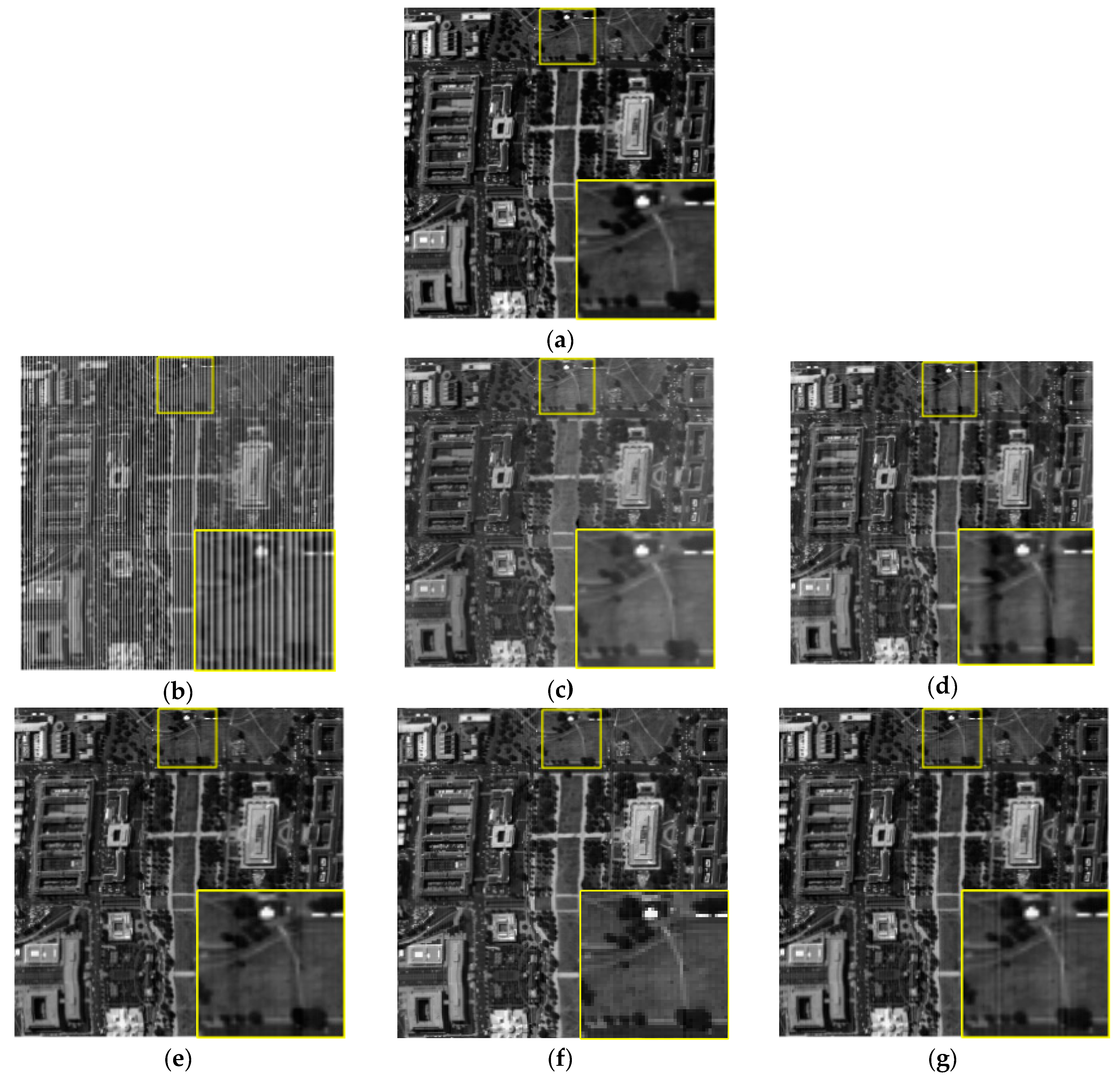

Figure 6.
Destriping results of band 5 for the non-periodic stripes case (r = 0.4 and I = 60): (a) original, (b) degraded with non-periodic stripes (case I = 60, r = 0.4), (c) UTV, (d) WFAF, (e) SGE, (f) ASSTV, (g) LRMID, (h) DL0S, (i) LRTD, and (j) GLTSA.
Figure 6.
Destriping results of band 5 for the non-periodic stripes case (r = 0.4 and I = 60): (a) original, (b) degraded with non-periodic stripes (case I = 60, r = 0.4), (c) UTV, (d) WFAF, (e) SGE, (f) ASSTV, (g) LRMID, (h) DL0S, (i) LRTD, and (j) GLTSA.
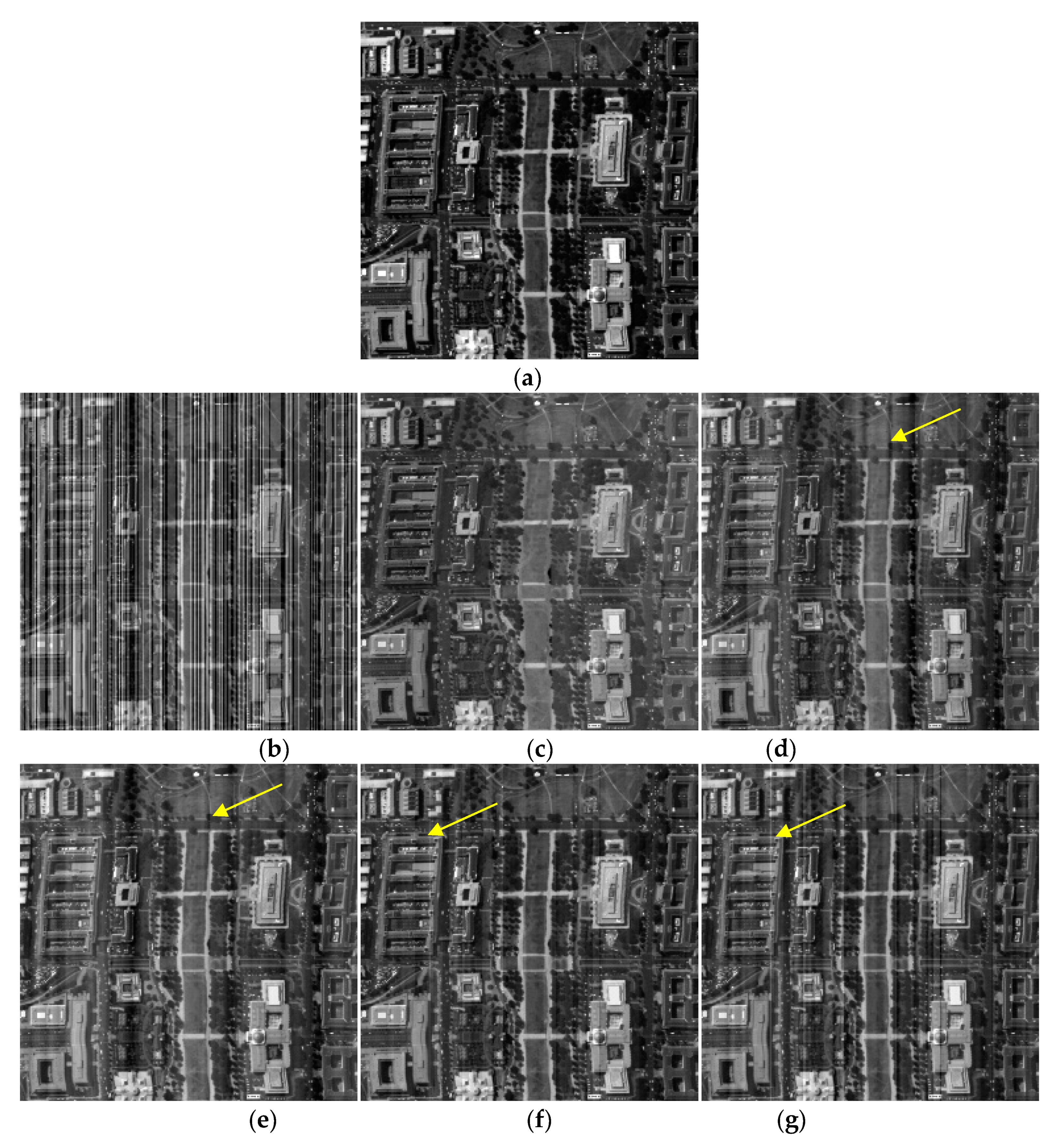

Figure 7.
(a) Degraded with periodic stripes (case I = 60, r = 0.8), (b) UTV, (c) WFAF, (d) SGE, (e) ASSTV, (f) LRMID, (g) DL0S, (h) LRTD, and (i) GLTSA.
Figure 7.
(a) Degraded with periodic stripes (case I = 60, r = 0.8), (b) UTV, (c) WFAF, (d) SGE, (e) ASSTV, (f) LRMID, (g) DL0S, (h) LRTD, and (i) GLTSA.

Figure 8.
(a) Degraded with non-periodic stripes (case I = 60, r = 0.4), (b) UTV, (c) WFAF, (d) SGE, (e) ASSTV, (f) LRMID, (g) DL0S, (h) LRTD, and (i) GLTSA.
Figure 8.
(a) Degraded with non-periodic stripes (case I = 60, r = 0.4), (b) UTV, (c) WFAF, (d) SGE, (e) ASSTV, (f) LRMID, (g) DL0S, (h) LRTD, and (i) GLTSA.

Figure 9.
Destriping results of the first real data 1. (a) Original; and destriping results by (b) UTV, (c) WFAF, (d) SGE, (e) ASSTV, (f) LRMID, (g) DL0S, (h) LRTD, and (i) GLTSA.
Figure 9.
Destriping results of the first real data 1. (a) Original; and destriping results by (b) UTV, (c) WFAF, (d) SGE, (e) ASSTV, (f) LRMID, (g) DL0S, (h) LRTD, and (i) GLTSA.

Figure 10.
Destriping results of the second real data. (a) Original; and destriping results by (b) UTV, (c) WFAF, (d) SGE, (e) ASSTV, (f) LRMID, (g) DL0S, (h) LRTD, and (i) GLTSA.
Figure 10.
Destriping results of the second real data. (a) Original; and destriping results by (b) UTV, (c) WFAF, (d) SGE, (e) ASSTV, (f) LRMID, (g) DL0S, (h) LRTD, and (i) GLTSA.

Figure 11.
Spatial mean cross-track profiles for the first real data: (a) original real image; and destriping results by (b) UTV, (c) WFAF, (d) SGE, (e) ASSTV, (f) LRMID, (g) DL0S, (h) LRTD, and (i) GLTSA.
Figure 11.
Spatial mean cross-track profiles for the first real data: (a) original real image; and destriping results by (b) UTV, (c) WFAF, (d) SGE, (e) ASSTV, (f) LRMID, (g) DL0S, (h) LRTD, and (i) GLTSA.
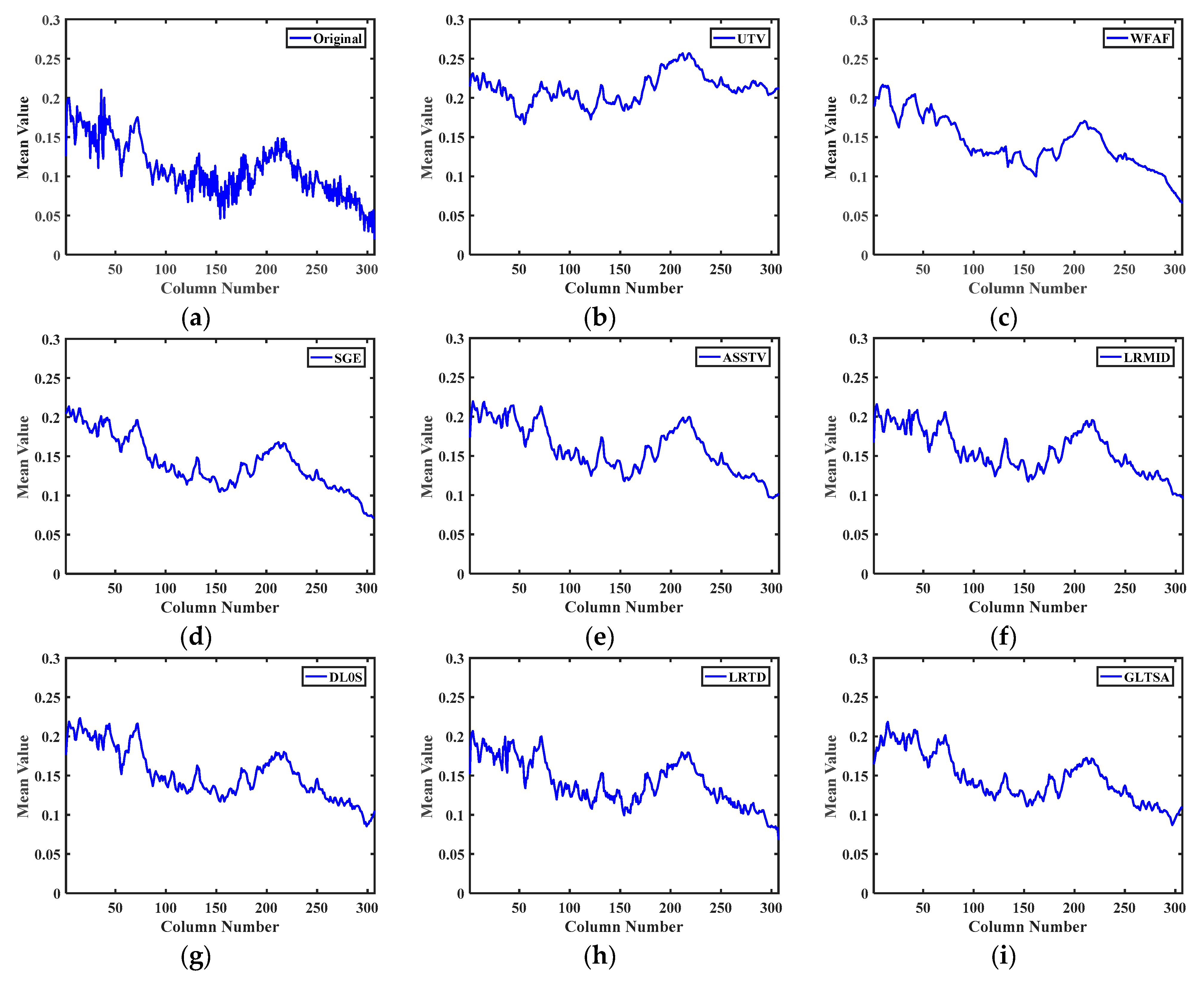
Figure 12.
Spatial mean cross-track profiles for the second real data: (a) real image; and destriping results by (b) UTV, (c) WFAF, (d) SGE, (e) ASSTV, (f) LRMID, (g) DL0S, (h) LRTD, and (i) GLTSA.
Figure 12.
Spatial mean cross-track profiles for the second real data: (a) real image; and destriping results by (b) UTV, (c) WFAF, (d) SGE, (e) ASSTV, (f) LRMID, (g) DL0S, (h) LRTD, and (i) GLTSA.
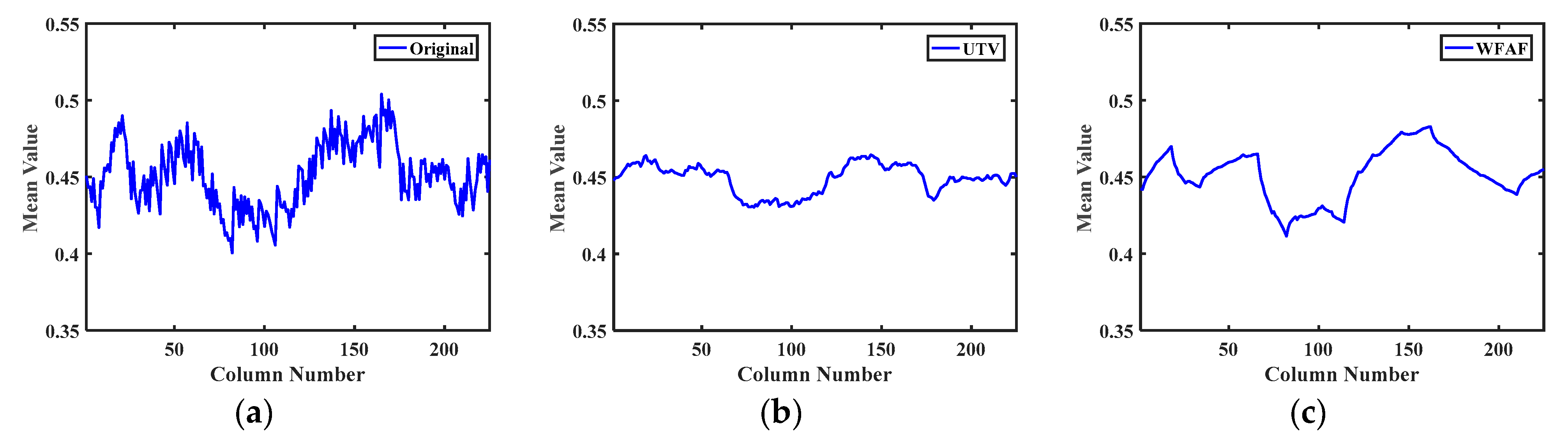

Figure 13.
The MPSNR curves as function of the regularization parameters. The relationship between MPSNR and the parameters (a) ; (b) ; (c) ; (d) ; (e) ; (f) ; (g) ; (h) .
Figure 13.
The MPSNR curves as function of the regularization parameters. The relationship between MPSNR and the parameters (a) ; (b) ; (c) ; (d) ; (e) ; (f) ; (g) ; (h) .


Figure 14.
MPSNR and MSSIM value versus the iteration number of GLTSA. (a) Change in the MPSNR value (periodic). (b) Change in the MSSIM value (periodic). (c) Change in the MPSNR value(non-periodic). (d) Change in the MSSIM value (non-periodic).
Figure 14.
MPSNR and MSSIM value versus the iteration number of GLTSA. (a) Change in the MPSNR value (periodic). (b) Change in the MSSIM value (periodic). (c) Change in the MPSNR value(non-periodic). (d) Change in the MSSIM value (non-periodic).

Table 1.
The mean values of indices of WDCM with periodic stripe.
| I | 20 | 60 | 100 | ||||||||||
|---|---|---|---|---|---|---|---|---|---|---|---|---|---|
| r | 0.2 | 0.4 | 0.8 | 0–1 | 0.2 | 0.4 | 0.8 | 0–1 | 0.2 | 0.4 | 0.8 | 0–1 | |
| MPSNR | Noisy | 29.10 | 26.09 | 23.08 | 26.51 | 19.56 | 16.55 | 13.54 | 15.28 | 15.12 | 12.11 | 9.10 | 11.94 |
| SGE [23] | 39.82 | 38.85 | 39.87 | 39.24 | 37.95 | 33.93 | 38.42 | 37.81 | 34.07 | 15.15 | 10.31 | 18.27 | |
| WFAF [22] | 31.58 | 31.36 | 31.51 | 31.36 | 31.08 | 29.59 | 30.43 | 30.52 | 30.29 | 27.39 | 28.87 | 29.01 | |
| UTV [14] | 25.85 | 25.85 | 25.85 | 25.84 | 25.85 | 25.84 | 25.85 | 25.85 | 25.85 | 25.84 | 25.85 | 25.85 | |
| ASSTV [19] | 36.70 | 36.70 | 36.34 | 36.57 | 36.70 | 36.71 | 34.64 | 36.17 | 36.72 | 36.73 | 32.07 | 36.18 | |
| LRMID [34] | 42.46 | 42.39 | 42.41 | 42.43 | 42.33 | 42.38 | 37.61 | 41.92 | 42.16 | 41.96 | 25.18 | 41.05 | |
| LRTD [20] | 49.86 | 48.85 | 42.10 | 47.86 | 49.81 | 48.95 | 41.76 | 48.98 | 49.81 | 49.01 | 41.66 | 48.67 | |
| DL0S [16] | 43.74 | 41.85 | 39.14 | 42.18 | 43.76 | 41.86 | 39.11 | 42.16 | 43.77 | 41.91 | 39.10 | 42.81 | |
| Ours | 50.90 | 47.95 | 42.55 | 48.28 | 54.22 | 47.97 | 42.33 | 50.19 | 53.79 | 50.12 | 42.32 | 50.94 | |
| MSSIM | Noisy | 0.8452 | 0.7429 | 0.5846 | 0.7752 | 0.5003 | 0.2883 | 0.1753 | 0.4235 | 0.3201 | 0.1185 | 0.0765 | 0.2894 |
| SGE [23] | 0.9907 | 0.988 | 0.9909 | 0.9906 | 0.9845 | 0.9602 | 0.9868 | 0.9764 | 0.9712 | 0.2951 | 0.1096 | 0.7698 | |
| WFAF [22] | 0.9483 | 0.9474 | 0.9484 | 0.9486 | 0.9469 | 0.9384 | 0.9456 | 0.9482 | 0.9441 | 0.9218 | 0.9398 | 0.9367 | |
| UTV [14] | 0.9022 | 0.9022 | 0.9022 | 0.9022 | 0.9022 | 0.9022 | 0.9022 | 0.9022 | 0.9021 | 0.9022 | 0.9021 | 0.9022 | |
| ASSTV [19] | 0.9833 | 0.9833 | 0.9812 | 0.9842 | 0.9833 | 0.9833 | 0.968 | 0.9846 | 0.9834 | 0.9834 | 0.9329 | 0.9792 | |
| LRMID [34] | 0.9954 | 0.9954 | 0.9955 | 0.9955 | 0.9953 | 0.9954 | 0.9802 | 0.9911 | 0.9949 | 0.9945 | 0.6796 | 0.9843 | |
| LRTD [20] | 0.999 | 0.9986 | 0.9941 | 0.9992 | 0.999 | 0.9987 | 0.9937 | 0.9979 | 0.999 | 0.9987 | 0.9936 | 0.9989 | |
| DL0S [16] | 0.9968 | 0.9951 | 0.9918 | 0.9978 | 0.9968 | 0.9951 | 0.9918 | 0.9952 | 0.9968 | 0.9951 | 0.9918 | 0.9966 | |
| Ours | 0.9988 | 0.9967 | 0.9942 | 0.9941 | 0.9995 | 0.9985 | 0.9948 | 0.9989 | 0.9995 | 0.9989 | 0.9948 | 0.9996 | |
| MFSIM | Noisy | 0.9271 | 0.856 | 0.8662 | 0.9158 | 0.8157 | 0.6427 | 0.694 | 0.8319 | 0.748 | 0.5372 | 0.6032 | 0.7384 |
| SGE [23] | 0.9927 | 0.9907 | 0.993 | 0.9928 | 0.9876 | 0.9714 | 0.9905 | 0.9901 | 0.9756 | 0.6516 | 0.6304 | 0.8542 | |
| WFAF [22] | 0.9626 | 0.9617 | 0.9623 | 0.9681 | 0.9605 | 0.954 | 0.9583 | 0.9598 | 0.9571 | 0.9418 | 0.9522 | 0.9568 | |
| UTV [14] | 0.9422 | 0.9422 | 0.9422 | 0.9422 | 0.9422 | 0.9422 | 0.9422 | 0.9422 | 0.9422 | 0.9422 | 0.9422 | 0.9422 | |
| ASSTV [19] | 0.9822 | 0.9822 | 0.9819 | 0.9823 | 0.9822 | 0.9822 | 0.9799 | 0.9831 | 0.9822 | 0.9823 | 0.9778 | 0.9818 | |
| LRMID [34] | 0.9965 | 0.9965 | 0.9966 | 0.9966 | 0.9963 | 0.9964 | 0.9932 | 0.9961 | 0.9958 | 0.9952 | 0.982 | 0.9967 | |
| LRTD [20] | 0.9994 | 0.9991 | 0.9969 | 0.9989 | 0.9993 | 0.9991 | 0.9966 | 0.9967 | 0.9993 | 0.9991 | 0.9965 | 0.9989 | |
| DL0S [16] | 0.9969 | 0.9956 | 0.9933 | 0.9958 | 0.9969 | 0.9956 | 0.9932 | 0.9958 | 0.9969 | 0.9956 | 0.9932 | 0.9959 | |
| Ours | 0.9989 | 0.9967 | 0.9955 | 0.9988 | 0.9996 | 0.998 | 0.9954 | 0.9989 | 0.9995 | 0.9988 | 0.9954 | 0.9992 | |
| SAM | Noisy | 0.177 | 0.356 | 0.452 | 0.378 | 0.387 | 0.776 | 0.931 | 0.814 | 0.494 | 0.991 | 1.139 | 1.024 |
| SGE [23] | 0.020 | 0.043 | 0.015 | 0.031 | 0.057 | 0.128 | 0.040 | 0.098 | 0.100 | 0.840 | 1.090 | 0.911 | |
| WFAF [22] | 0.025 | 0.048 | 0.030 | 0.038 | 0.053 | 0.122 | 0.065 | 0.079 | 0.080 | 0.186 | 0.097 | 0.137 | |
| UTV [14] | 0.049 | 0.049 | 0.049 | 0.049 | 0.050 | 0.050 | 0.051 | 0.051 | 0.051 | 0.052 | 0.052 | 0.052 | |
| ASSTV [19] | 0.035 | 0.035 | 0.035 | 0.035 | 0.035 | 0.035 | 0.035 | 0.035 | 0.035 | 0.035 | 0.036 | 0.035 | |
| LRMID [34] | 0.038 | 0.039 | 0.039 | 0.039 | 0.040 | 0.040 | 0.050 | 0.046 | 0.042 | 0.045 | 0.169 | 0.064 | |
| LRTD [20] | 0.023 | 0.026 | 0.033 | 0.029 | 0.023 | 0.026 | 0.033 | 0.028 | 0.023 | 0.026 | 0.033 | 0.029 | |
| DL0S [16] | 0.011 | 0.021 | 0.028 | 0.023 | 0.011 | 0.021 | 0.028 | 0.019 | 0.011 | 0.021 | 0.028 | 0.018 | |
| Ours | 0.013 | 0.027 | 0.030 | 0.025 | 0.006 | 0.017 | 0.031 | 0.013 | 0.007 | 0.012 | 0.031 | 0.014 | |
| ERGAS | Noisy | 131.10 | 185.40 | 262.20 | 241.61 | 393.29 | 556.19 | 786.59 | 581.47 | 655.48 | 926.98 | 1311.0 | 986.87 |
| SGE [23] | 38.16 | 42.68 | 37.96 | 39.58 | 47.46 | 75.30 | 44.83 | 56.24 | 77.76 | 653.70 | 1141.4 | 878.94 | |
| WFAF [22] | 98.71 | 101.21 | 99.50 | 100.98 | 104.69 | 124.43 | 112.74 | 118.36 | 115.71 | 161.12 | 135.79 | 152.68 | |
| UTV [14] | 191.27 | 191.27 | 191.27 | 191.27 | 191.28 | 191.33 | 191.29 | 191.30 | 191.30 | 191.44 | 191.33 | 191.38 | |
| ASSTV [19] | 56.22 | 56.20 | 58.38 | 56.28 | 56.19 | 56.14 | 70.14 | 59.34 | 56.09 | 56.00 | 93.45 | 65.97 | |
| LRMID [34] | 30.80 | 31.00 | 31.00 | 30.91 | 31.37 | 31.08 | 49.89 | 35.94 | 31.91 | 32.16 | 205.92 | 49.78 | |
| LRTD [20] | 17.11 | 19.05 | 31.03 | 24.61 | 17.15 | 19.04 | 32.06 | 26.25 | 17.15 | 19.03 | 32.38 | 29.37 | |
| DL0S [16] | 24.68 | 30.42 | 41.73 | 32.84 | 24.62 | 30.34 | 41.98 | 36.27 | 24.56 | 30.18 | 42.00 | 38.57 | |
| Ours | 10.83 | 18.95 | 29.04 | 21.06 | 7.46 | 20.51 | 30.66 | 23.58 | 7.89 | 12.42 | 30.69 | 26.75 |
The boldface digits in Table 2 represent the best results.
Table 2.
The mean values of indices of WDCM with non-periodic stripe.
| I | 20 | 60 | 100 | ||||||||||
|---|---|---|---|---|---|---|---|---|---|---|---|---|---|
| R | 0.2 | 0.4 | 0.8 | 0–1 | 0.2 | 0.4 | 0.8 | 0–1 | 0.2 | 0.4 | 0.8 | 0–1 | |
| MPSNR | Noisy | 29.12 | 26.09 | 23.08 | 27.13 | 19.58 | 16.55 | 13.54 | 17.34 | 15.14 | 12.12 | 9.1 | 12.85 |
| SGE [23] | 37.05 | 36.28 | 34.01 | 36.89 | 30.18 | 28.47 | 23.41 | 29.19 | 22.59 | 16.29 | 9.97 | 17.92 | |
| WFAF [22] | 31.12 | 30.78 | 30.19 | 30.85 | 28.41 | 26.97 | 25.07 | 27.38 | 25.63 | 23.63 | 21.3 | 24.11 | |
| UTV [14] | 25.85 | 25.84 | 25.82 | 25.84 | 25.84 | 25.74 | 25.62 | 25.78 | 25.83 | 25.55 | 25.29 | 25.68 | |
| ASSTV [19] | 35.83 | 35.97 | 34.22 | 36.12 | 32.15 | 31.37 | 26.86 | 31.62 | 28.48 | 26.83 | 21.84 | 27.38 | |
| LRMID [34] | 39.72 | 39.66 | 35.95 | 39.67 | 32.47 | 30.33 | 25.26 | 31.95 | 27.22 | 24.28 | 19.51 | 25.91 | |
| LRTD [20] | 47.88 | 43.96 | 30.5 | 44.98 | 47.78 | 42.34 | 23.36 | 44.68 | 47.85 | 40.23 | 19.56 | 41.38 | |
| DL0S [16] | 42.88 | 41.3 | 31.45 | 42.88 | 42.87 | 40.94 | 26.98 | 41.67 | 42.11 | 37.68 | 23.13 | 40.62 | |
| Ours | 48.59 | 43.52 | 36.44 | 46.25 | 53.01 | 42.81 | 31.09 | 47.39 | 52.52 | 46.9 | 26.24 | 47.19 | |
| MSSIM | Noisy | 0.8599 | 0.7598 | 0.6133 | 0.8367 | 0.5333 | 0.336 | 0.1664 | 0.4168 | 0.3684 | 0.1716 | 0.0552 | 0.2168 |
| SGE [23] | 0.9871 | 0.9858 | 0.979 | 0.9862 | 0.9524 | 0.9334 | 0.8209 | 0.9258 | 0.8191 | 0.5056 | 0.0767 | 0.6729 | |
| WFAF [22] | 0.9457 | 0.9443 | 0.9425 | 0.9455 | 0.9216 | 0.9088 | 0.8864 | 0.9094 | 0.8786 | 0.8429 | 0.7849 | 0.8581 | |
| UTV [14] | 0.9022 | 0.9022 | 0.902 | 0.9021 | 0.9022 | 0.901 | 0.8994 | 0.9011 | 0.902 | 0.8986 | 0.8936 | 0.8988 | |
| ASSTV [19] | 0.9801 | 0.9805 | 0.9719 | 0.9779 | 0.9555 | 0.9432 | 0.8569 | 0.9412 | 0.8965 | 0.8448 | 0.6567 | 0.8567 | |
| LRMID [34] | 0.9923 | 0.9918 | 0.9808 | 0.9919 | 0.9552 | 0.9174 | 0.7831 | 0.9239 | 0.851 | 0.7309 | 0.4985 | 0.7862 | |
| LRTD [20] | 0.9985 | 0.9962 | 0.9373 | 0.9968 | 0.9985 | 0.9948 | 0.8043 | 0.9913 | 0.9985 | 0.9922 | 0.6691 | 0.9936 | |
| DL0S [16] | 0.9963 | 0.9946 | 0.9736 | 0.9949 | 0.9962 | 0.9945 | 0.9402 | 0.9938 | 0.9952 | 0.9909 | 0.8781 | 0.9917 | |
| Ours | 0.9991 | 0.9961 | 0.9884 | 0.9989 | 0.9994 | 0.9958 | 0.9733 | 0.9987 | 0.9993 | 0.9979 | 0.9299 | 0.9981 | |
| MFSIM | Noisy | 0.9317 | 0.8819 | 0.8275 | 0.8897 | 0.8104 | 0.7021 | 0.6324 | 0.7168 | 0.7421 | 0.6159 | 0.5437 | 0.6348 |
| SGE [23] | 0.9912 | 0.9906 | 0.9867 | 0.9921 | 0.9771 | 0.9667 | 0.9065 | 0.9698 | 0.9066 | 0.7551 | 0.5874 | 0.7965 | |
| WFAF [22] | 0.9616 | 0.9611 | 0.9597 | 0.9612 | 0.9542 | 0.9488 | 0.9369 | 0.9514 | 0.9421 | 0.9285 | 0.9043 | 0.9341 | |
| UTV [14] | 0.9422 | 0.9422 | 0.9422 | 0.9422 | 0.9422 | 0.9422 | 0.9422 | 0.9422 | 0.9422 | 0.9422 | 0.9422 | 0.9422 | |
| ASSTV [19] | 0.98 | 0.9803 | 0.9759 | 0.9796 | 0.9664 | 0.9585 | 0.9111 | 0.9559 | 0.9359 | 0.9082 | 0.8165 | 0.9167 | |
| LRMID [34] | 0.9946 | 0.9945 | 0.9873 | 0.9937 | 0.9705 | 0.651 | 0.8784 | 0.9367 | 0.9144 | 0.8628 | 0.7514 | 0.8934 | |
| LRTD [20] | 0.9988 | 0.9969 | 0.9619 | 0.9971 | 0.9988 | 0.9955 | 0.8802 | 0.9959 | 0.9988 | 0.9935 | 0.8022 | 0.9945 | |
| DL0S [16] | 0.9966 | 0.9955 | 0.9848 | 0.9962 | 0.9966 | 0.9954 | 0.9751 | 0.9956 | 0.9963 | 0.9942 | 0.9533 | 0.9939 | |
| Ours | 0.9993 | 0.9965 | 0.9918 | 0.9989 | 0.9995 | 0.9962 | 0.9884 | 0.9981 | 0.9993 | 0.9981 | 0.9772 | 0.9979 | |
| SAM | Noisy | 0.187 | 0.309 | 0.44 | 0.338 | 0.447 | 0.706 | 0.921 | 0.769 | 0.593 | 0.912 | 1.129 | 0.927 |
| SGE [23] | 0.063 | 0.081 | 0.107 | 0.089 | 0.187 | 0.237 | 0.4 | 0.243 | 0.387 | 0.732 | 1.1 | 0.933 | |
| WFAF [22] | 0.066 | 0.086 | 0.1 | 0.088 | 0.183 | 0.236 | 0.269 | 0.247 | 0.29 | 0.365 | 0.419 | 0.387 | |
| UTV [14] | 0.05 | 0.054 | 0.058 | 0.056 | 0.056 | 0.087 | 0.111 | 0.091 | 0.066 | 0.126 | 0.166 | 0.134 | |
| ASSTV [19] | 0.035 | 0.035 | 0.035 | 0.035 | 0.037 | 0.035 | 0.081 | 0.051 | 0.068 | 0.068 | 0.231 | 0.098 | |
| LRMID [34] | 0.04 | 0.039 | 0.041 | 0.040 | 0.053 | 0.06 | 0.153 | 0.073 | 0.122 | 0.184 | 0.387 | 0.214 | |
| LRTD [20] | 0.023 | 0.027 | 0.055 | 0.037 | 0.023 | 0.027 | 0.188 | 0.068 | 0.023 | 0.026 | 0.3 | 0.187 | |
| DL0S [16] | 0.016 | 0.031 | 0.139 | 0.069 | 0.016 | 0.034 | 0.236 | 0.088 | 0.024 | 0.061 | 0.362 | 0.195 | |
| Ours | 0.015 | 0.027 | 0.057 | 0.028 | 0.007 | 0.015 | 0.148 | 0.041 | 0.008 | 0.017 | 0.275 | 0.086 | |
| ERGAS | Noisy | 131.20 | 185.49 | 262.28 | 188.39 | 393.61 | 556.4 | 786.85 | 586.24 | 656.01 | 927.46 | 1311.4 | 951.44 |
| SGE [23] | 52.87 | 57.43 | 74.51 | 60.12 | 117.20 | 141.0 | 261.77 | 156.85 | 282.73 | 581.81 | 1187.8 | 786.75 | |
| WFAF [22] | 103.96 | 108.04 | 115.9 | 109.87 | 143.46 | 167.88 | 210.53 | 189.67 | 200.30 | 247.29 | 325.82 | 258.97 | |
| UTV [14] | 191.23 | 191.52 | 191.81 | 191.64 | 191.35 | 193.56 | 196.04 | 194.35 | 191.69 | 197.60 | 204.23 | 197.64 | |
| ASSTV [19] | 61.60 | 60.54 | 73.4 | 62.88 | 92.64 | 101.09 | 169.59 | 121.07 | 140.85 | 170.36 | 302.18 | 188.69 | |
| LRMID [34] | 39.81 | 40.06 | 59.9 | 42.81 | 89.02 | 113.91 | 203.93 | 128.94 | 162.79 | 228.39 | 395.39 | 235.67 | |
| LRTD [20] | 18.85 | 25.83 | 111.55 | 61.86 | 18.94 | 29.99 | 253.94 | 94.38 | 18.89 | 37.27 | 393.12 | 125.74 | |
| DL0S [16] | 27.11 | 32.40 | 101.17 | 58.94 | 27.20 | 33.81 | 169.91 | 87.14 | 31.19 | 51.03 | 264.12 | 119.68 | |
| Ours | 15.07 | 25.11 | 56.66 | 30.45 | 9.36 | 28.16 | 105.40 | 56.97 | 9.81 | 17.96 | 188.68 | 86.47 |
The boldface digits in Table 2 represent the best results.
Table 3.
The MICV and MMRD index results of the real data experiments.
| Dataset | Index | UTV | WFAF | SGE | ASSTV | LRMID | DL0S | LRTD | GLTSA |
|---|---|---|---|---|---|---|---|---|---|
| (1) | MICV | 28.176 | 60.871 | 58.947 | 90.526 | 98.618 | 118.856 | 110.054 | 121.248 |
| MMRD (%) | 0.2013 | 0.1504 | 0.1706 | 0.1206 | 0.0951 | 0.0538 | 0.0864 | 0.0547 | |
| (2) | MICV | 16.315 | 31.056 | 30.842 | 36.118 | 46.211 | 53.137 | 53.204 | 52.176 |
| MMRD (%) | 0.0913 | 0.0844 | 0.0901 | 0.0628 | 0.0251 | 0.0198 | 0.0365 | 0.0139 |
Table 4.
Comparison of running time on WDCM dataset with periodic and non-periodic stripe (in seconds).
Table 4.
Comparison of running time on WDCM dataset with periodic and non-periodic stripe (in seconds).
| Stripe Type | UTV | WFAF | SGE | ASSTV | LRMID | DL0S | LRTD | GLTSA |
|---|---|---|---|---|---|---|---|---|
| Periodic | 10.94 | 8.89 | 3.99 | 92.14 | 209.12 | 179.85 | 785.98 | 182.33 |
| non-periodic | 11.23 | 9.18 | 4.37 | 95.33 | 214.51 | 183.64 | 789.46 | 186.75 |
© 2020 by the authors. Licensee MDPI, Basel, Switzerland. This article is an open access article distributed under the terms and conditions of the Creative Commons Attribution (CC BY) license (http://creativecommons.org/licenses/by/4.0/).
Share and Cite
MDPI and ACS Style
Kong, X.; Zhao, Y.; Xue, J.; Chan, J.C.-W.; Kong, S.G. Global and Local Tensor Sparse Approximation Models for Hyperspectral Image Destriping. Remote Sens. 2020, 12, 704. https://0-doi-org.brum.beds.ac.uk/10.3390/rs12040704
AMA Style
Kong X, Zhao Y, Xue J, Chan JC-W, Kong SG. Global and Local Tensor Sparse Approximation Models for Hyperspectral Image Destriping. Remote Sensing. 2020; 12(4):704. https://0-doi-org.brum.beds.ac.uk/10.3390/rs12040704
Chicago/Turabian StyleKong, Xiangyang, Yongqiang Zhao, Jize Xue, Jonathan Cheung-Wai Chan, and Seong G. Kong. 2020. "Global and Local Tensor Sparse Approximation Models for Hyperspectral Image Destriping" Remote Sensing 12, no. 4: 704. https://0-doi-org.brum.beds.ac.uk/10.3390/rs12040704
Note that from the first issue of 2016, this journal uses article numbers instead of page numbers. See further details here.