
Compound Multiscale Weak Dense Network with Hybrid Attention for Hyperspectral Image Classification


1
School of Computer Science and Engineering, Nanjing University of Science and Technology, Nanjing 210094, China
2
Jiangsu Key Laboratory of Broadband Wireless Communication and Internet of Things, Nanjing University of Posts and Telecommunications, Nanjing 210003, China
3
School of Internet of Things, Nanjing University of Posts and Telecommunications, Nanjing 210003, China
*
Author to whom correspondence should be addressed.
Remote Sens. 2021, 13(16), 3305; https://0-doi-org.brum.beds.ac.uk/10.3390/rs13163305
Submission received: 12 July 2021
/
Revised: 17 August 2021
/
Accepted: 18 August 2021
/
Published: 20 August 2021
Abstract
:Recently, hyperspectral image (HSI) classification has become a popular research direction in remote sensing. The emergence of convolutional neural networks (CNNs) has greatly promoted the development of this field and demonstrated excellent classification performance. However, due to the particularity of HSIs, redundant information and limited samples pose huge challenges for extracting strong discriminative features. In addition, addressing how to fully mine the internal correlation of the data or features based on the existing model is also crucial in improving classification performance. To overcome the above limitations, this work presents a strong feature extraction neural network with an attention mechanism. Firstly, the original HSI is weighted by means of the hybrid spectral–spatial attention mechanism. Then, the data are input into a spectral feature extraction branch and a spatial feature extraction branch, composed of multiscale feature extraction modules and weak dense feature extraction modules, to extract high-level semantic features. These two features are compressed and fused using the global average pooling and concat approaches. Finally, the classification results are obtained by using two fully connected layers and one Softmax layer. A performance comparison shows the enhanced classification performance of the proposed model compared to the current state of the art on three public datasets.

1. Introduction
Hyperspectral remote sensing, namely, hyperspectral-resolution remote sensing, refers to the use of many very narrow electromagnetic wave segments (usually <10 nm) to obtain relevant data from the target area. The HSI is acquired using an imaging spectrometer that provides detailed spectral information in a narrow range of continuous wavelengths [1]. Benefitting from the high spectral resolution, the resulting HSI shows advantages in identifying various land-cover categories or targets [2]. It enables substances that cannot be detected in wideband remote sensing to be detected in hyperspectral data.
In recent years, due to the high dimension and massive data of HSIs, the analysis and processing of HSIs has become one of the hotspots in remote sensing image research. The process has been widely used in ocean detection [3,4], mineral exploration [5,6], road detection [7], vegetation analysis [8,9], national defense and military applications [10,11], etc., and it is worthy of further research.
The difference between HSI and RGB images is that an HSI divides the spectral dimension in a very detailed way based on an RGB image, and then forms a three-dimensional data cube with multiple bands stacked in sequence. HSI classification refers to analyzing the spectral and spatial information of all categories of ground objects in the HSI, selecting the features, dividing the feature space into non-overlapping subspace through various methods, and then dividing each pixel in the image into each subspace.
In recent decades, deep learning technology [12,13,14] has become one of the most popular research fields in artificial intelligence. It has made breakthroughs in many fields such as image processing [15,16], speech recognition [17], natural language processing [18], and so on. It is currently one of the most advantageous technologies applied to HSI classification tasks. Based on the particularity of HSIs, many spectral bands and neighborhood pixels of the target pixel all contain significant features. The effective use of the spectral and spatial information of the data is the key to extracting robust and discriminative features. A 3D CNN has the characteristics of parameter sharing and local perception, which fit the special research requirements of HSIs. Therefore, most of the classification models proposed in recent years are based on the 3D CNN approach. Lee et al. [19] proposed a contextual deep CNN, which jointly utilizes the local spectral–spatial relationship of adjacent single pixels to optimally explore local contextual interactions. Zhong et al. [20] designed an end-to-end spectral–spatial residual network, which uses residual connections to reduce decreases in accuracy caused by increases in network depth. Wang et al. [21] proposed an end-to-end fast dense spectral–spatial convolution model, which combines different convolution kernel scales with dense connections in order to extract features. Roy et al. [22] used a hybrid 2D-3D CNN to construct a lightweight end-to-end network model. Ge et al. [23] constructed a multiscale multibranch feature-fusion HSI classification model based on a 2D-3D CNN, and achieved a good classification performance. Huang et al. [24] proposed a dual-path Siamese CNN for HSI classification. This model integrates morphological profiles, a CNN, a Siamese network, and spectral–spatial feature extraction technology, and achieves good classification results. Safari et al. [25] designed a neural network that combines different convolution kernels to effectively learn joint spatial–spectral features on a multiscale, which achieves better classification effects on high-resolution datasets. Praveen et al. [26] proposed a classification model combining traditional methods with CNN, and achieved good performance. In [27], a lightweight spectral–spatial convolution model was proposed to replace the convolution layer. This model consists of cheap transformation operations, which can greatly reduce the model parameters. Gao et al. [28] proposed a sandwich CNN based on spectral feature enhancement (SFE-SCNN), which reduces the interference of mixed pixels by enhancing spectral features.
How to mine the internal correlations of data or features has become a research hotspot in recent years, with researchers focusing on introducing an attention mechanism to weight data or features to improve the information utilization. The attention mechanism was initially used to deal with computation vision tasks [29,30,31] and showed good performance. For HSI classification tasks, attention mechanisms are also effective. Typically, attention mechanisms are added at the beginning or end of the neural network models. According to their position in the model, they can be divided into preprocessing-based attention mechanisms and postprocessing-based attention mechanisms.
The attention mechanism based on preprocessing is generally located at the initial stage of the model, directly processing the original HSI data and mining the structural characteristics of the original data [32,33,34]. Yu et al. [35] proposed a spectral–spatial dense CNN model with a feedback attention mechanism, using the semantic knowledge provided by the high level of the dense model to enhance the attention map. Zhu et al. [36] proposed an end-to-end residual spectral–spatial attention network. Based on the residual spectral attention module and spatial attention module, the original hyperspectral data are processed and fed into the CNN for feature extraction. Lin et al. [37] designed an attention-aware pseudo-3D CNN model, which provides a more detailed description of each dimension of the input by allocating attention. Guo et al. [38] proposed a feature-grouped network based on a spectral–spatial connected attention mechanism (FG-SSCA) to enhance the effectiveness of the data.
The attention mechanism based on postprocessing is usually located in the middle or end of the model, which improves the feature utilization by weighting high-dimensional semantic features. Ma et al. [39] constructed a double-branch multi-attention mechanism network (DBMA). The extracted features are weighted via the spectral and spatial attention modules for better classification performance. Compared with DBMA, DBDA [40] introduced a more flexible and adaptive attention mechanism to achieve better classification performance, while keeping the overall network architecture unchanged. In [41], a 3-D octave convolution (3D-OC) approach combined with a spectral–spatial attention network was proposed to extract discriminative spectral–spatial features. A 3D-OC first mines deep spatial information from high to low frequencies, and also takes spectral information into account. Then, two attention modules are used to highlight important spatial regions and special spectral bands to improve feature discrimination. Xue et al. [42] designed a second-order pooling network based on the attention mechanism, which assigns different weights to different pixels through a correlation matrix and a learnable cosine distance function. Zhang et al. [43] proposed a spectral–spatial–semantic network, which combines a multi-directional attention mechanism for HSI classification. Pu et al. [44] presented a dual-path CNN model based on an attention mechanism, which adaptively recalibrates the nonlinear interdependence between features in conjunction with the multiscale attention mechanism (MS-AM) to alleviate the Hughes phenomenon. Cui et al. [45] proposed a dual–triple attention network model, which achieves the high classification accuracy of HSIs by capturing cross-dimensional interactive information. In this model, attention mechanisms are added during and after the feature extraction process to improve the effectiveness of features. Zhao et al. [46] proposed a central attention network to effectively understand the internal correlation between the central pixel and its neighborhood pixels in a subcube sample. The spectral–spatial features generated by this method showed good discrimination performance. Xue et al. [47] proposed a hierarchical residual network with an attention mechanism (HResNetAM), which uses attention mechanisms in the spectral and spatial feature extraction branches to calibrate the weights of hierarchical spectral and spatial features.
In this paper, inspired by these advanced methods, we propose a novel compound multiscale weak dense network to extract strong, robust and discriminative features. In the preprocessing stage, we construct a hybrid attention mechanism to improve data effectiveness. Our new deep model consists of two network branches to extract the spectral and spatial features of HSI, respectively. For each branch of the network, the compound multiscale feature extraction modules are designed to obtain abundant features at different scales. Then, the weak dense feature extraction modules are constructed to further extract more discriminative high-dimensional semantic features. Through concat, we fuse the features of the two branches. Finally, the fused spectral–spatial features are fed into fully connected layers and a Softmax layer to obtain the classification results. In addition, in order to further enhance the performance of the model, a learnable hybrid spectral–spatial attention mechanism is designed for data preprocessing.
The main contributions of this paper are as follows:
- (1)
- A compound multiscale weak dense network model combining a hybrid attention mechanism (CMWD-HA) is proposed for HSI classification. This model shows good classification performance and high efficiency;
- (2)
- A hybrid spectral–spatial attention mechanism is proposed in preprocessing. This attention mechanism aims to weight HSI data simultaneously at both spectral and spatial levels. In addition, the mechanism is learnable and consumes fewer computing resources;
- (3)
- Spectral and spatial multiscale feature extraction modules and weak dense spectral and spatial feature extraction modules are designed, and spectral feature extraction branches and spatial feature extraction branches are constructed based on the above modules. The extracted high-level semantic features can distinguish different categories of pixels well, with good generalization ability;
- (4)
- Dropout and dynamic learning rates are used to ensure the rapid convergence of the model.
2. Related Work
ResNet and DenseNet
In deep learning models, the shallow network layers may not fit the data well, resulting in weak performance. When the number of network layers increases to some extent, the performance of the model is enhanced accordingly. However, as the number of network layers increases, some corresponding problems appear. For example, the huge consumption of computing resources, the overfitting problem, the gradient disappears, the gradient explodes, and so on. The performance of the model is not always positively correlated with the increase in the number of network layers. When the number of network layers increases to a certain range, the network experiences degradation. That is, as the number of network layers increases, the loss of the training set gradually decreases. When the network depth continues to increase, the loss will increase instead. When network degradation occurs, the training effect of a shallow network is better than that of a deep network [48]. For the data processing inequality in information theory, that is, for a Markov process X → Y → Z, there exists I(X; Y) ≧ I(X; Z), where I represents mutual information. Therefore, in forward propagation, the deeper the number of network layers, the less original information the feature contains. Model performance cannot be improved by continuously increasing network depth. At this time, if the low-level features are transferred to the high level, the effect of the model will at least be no worse than that of the shallow network, which is the reason that ResNet was proposed. ResNet guarantees that the network of the N + 1 layer contains more image information than the N layer. The computation equation of ResNet is as follows:
where xl represents the output of the l layer, and Hl represents a nonlinear transformation. For ResNet, the output of layer l is the output of layer l − 1 plus the nonlinear transformation of the output of layer l − 1.
DenseNet [49] is based on a similar idea to that of ResNet, but it creates dense connections between all the previous layers and the back layers. The proposal of DenseNet fully reuses the features, that is, each layer of the network can use the feature maps of all previous layers. Compared to ResNet, DenseNet promotes gradient backpropagation, making the network easier to train. In addition, DenseNet can achieve better performance than ResNet with fewer parameters and lower computing costs. The computation equation of DenseNet is as follows:
where xl represents the output of l layer, Hl is a nonlinear transformation, and [] indicates concat of the output feature maps from layer 0 to l − 1.
Figure 1a shows the connection mechanism of ResNet, and Figure 1b shows DenseNet. ResNet is the element-level addition between the input of each layer and the input of the previous layer. In DenseNet, each layer is connected with all the previous layers through dimensional stacking (concat). For an L-layer network, DenseNet contains L(L + 1)/2 connections, whereas ResNet contains L connections.
3. Methodology
3.1. Hybrid Attention Mechanism
The attention mechanism is a data processing method in machine learning, which has been widely used in natural language processing [50,51] and image processing [52,53]. In HSI processing tasks, scholars have further improved the performance of the model by introducing attention mechanisms based on the study of a neural network model. The attention mechanism can help the model to assign different weights to each part of the input, extract more critical and important information, and enable the model to make more accurate judgments without exerting too much calculation and storage pressure.
This paper proposes a hybrid attention mechanism, which is located at the beginning of the network model. From the perspective of a hybrid and learnable approach, we designed the hybrid attention mechanism to accomplish both spectral and spatial attention simultaneously. The flowchart of the hybrid attention mechanism is shown in Figure 2, taking the Indian Pines dataset as an example. After carrying out principal component analysis (PCA) for dimension reduction, the dimensions of the original data cube change from 15 × 15 × 200 to 15 × 15 × 30. According to the spectral branch and spatial branch in the hybrid attention mechanism, the data are processed into 1 × 1 × 30 and 15 × 15 × 1 through AveragePooling3D. Then, the data are constrained between 0 and 1 through the sigmoid function after a 2D convolution. Among these, the scales of 2D convolution kernels in the spectral branch and spatial branch are 1 × 1 and 3 × 3, respectively. After sigmoid processing, the attention matrix of the same dimension as the original data is obtained through matrix multiplication of the data of the two branches. Finally, the original data and the attention matrix are multiplied element by element and added to complete the attention process.
3.2. Multiscale Spectral and Spatial Feature Extraction
HSI cubes exhibit the phenomena of “same spectral, different material”, and “same material, different spectral”, meaning that single-scale features cannot reflect the characteristics of image pixels well. Therefore, we propose a multiscale spectral feature extraction module and a multiscale spatial feature extraction module, respectively. In this way, more local and more global features can be considered. As shown in Figure 3a, for the multiscale spectral feature extraction module, HSI image cubes are processed by 3D convolutional layers with scales of 1 × 1 × 3, 1 × 1 × 5, and 1 × 1 × 7, respectively, and then fused by concat. Finally, feature alignment is performed through a 3D CNN with a kernel scale of 7 × 7 × 7. The multiscale spatial feature extraction module is shown in Figure 3b. We designed three branches of the neural network to extract multiscale spatial features of the image cubes. The first branch uses a 3D CNN with the kernel scale of 7 × 7 × 7, and the second branch uses two layers of a 3D CNN with the kernel scales of 5 × 5 × 5 and 3 × 3 × 3. The third branch uses three layers of a 3D CNN with the same kernel scale of 3 × 3 × 3. Then, the feature maps extracted from the three branches are also fused through concat. Finally, feature alignment is also performed by means of a 3D CNN with a kernel scale of 1 × 1 × 1. So far, multiscale spectral features and multiscale spatial features have been extracted, respectively. The implementation details of two multiscale feature extraction modules are shown in Table 1 and Table 2.
3.3. Weak Dense Spectral and Spatial Feature Extraction
After multiscale spectral and spatial feature extraction, the features are fed into the weak dense spectral and spatial feature extraction modules, respectively. In this part of the process, we weaken the DenseNet structure and only retain skip connections between adjacent network layers. The input of each network layer is the fusion of the output feature maps of the previous two network layers. Padding processing is applied to the feature maps in these two modules to ensure that the dimensions of the feature maps remain unchanged. In addition, the stride of the last two convolution layers of each module is set to (1,1,2). The weak dense structure reduces the dimensions of the feature maps while ensuring the reuse of the feature, which improves the model’s efficiency to some extent. The implementation details of two weak dense modules are shown in Table 3 and Table 4.
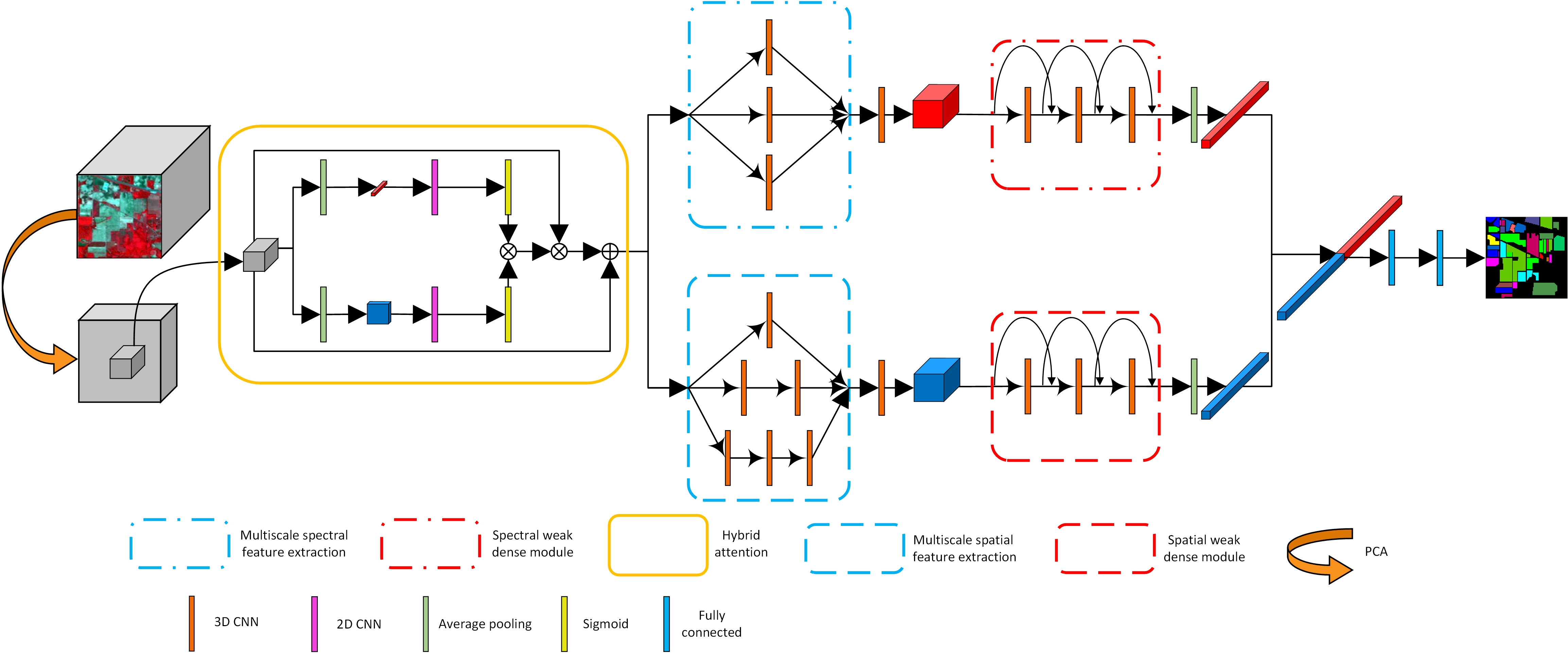
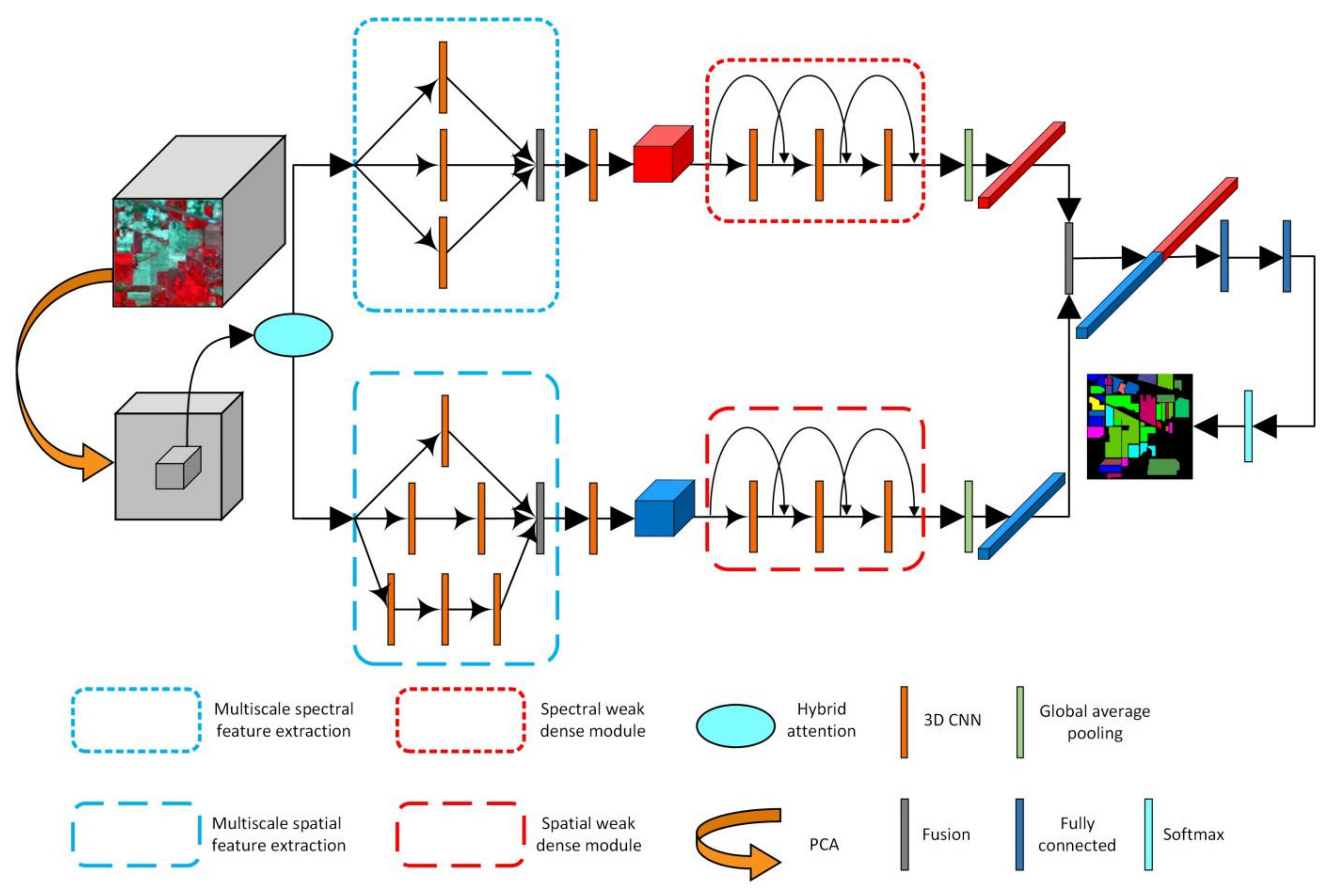
3.4. Compound Multiscale Weak Dense Network with Hybrid Attention for HSI Classification
The structure of our CMWD-HA is shown in Figure 4. This model can be divided into two parts: the data preprocessing stage and the feature extraction and classification stage. In the data preprocessing stage, the original HSI is processed by means of PCA for dimension reduction, and the hybrid attention mechanism is adopted to assign corresponding weights to the data to improve the effectiveness of the data. After PCA processing of HSI, the data are compressed in the spectral dimension, and the influence of noise and redundant information is greatly reduced. At this time, the hyperspectral data still have dozens of spectral bands, and the spectral information for different categories of pixels is still discriminative. Therefore, implementing the spectral–spatial attention mechanism on the PCA-processed data can enhance the effectiveness of the data, thereby improving the classification performance of the model. For the feature extraction and classification stage, the proposed method constructs two neural network branches. The two branches first extract the multiscale spectral and spatial features of HSI, and then use the weak dense feature extraction modules to extract high-dimensional semantic features with sufficient discrimination. The data, processed by PCA and the attention mechanism, have abundant spectral and spatial information, and the important information in the data is more prominent. At this time, based on the multiscale spectral and multiscale spatial attention modules, very rich spectral and spatial features can be obtained. Then, combining these with the weak dense feature extraction modules, the model can extract higher-dimensional and more abstract semantic features. This ensures that the subsequent fusion features exhibit strong discrimination and can accurately complete the classification task. Finally, global average pooling is used to reduce the dimensions of features in two branches, and then two features are fused. The classification results are obtained through two fully connected layers and a Softmax layer.
3.5. Measures Taken to Prevent Overfitting
In the construction of deep learning models, if we blindly attempt to improve the predictive ability of model, the complexity of the structure will often be relatively high. Generally speaking, deep learning models contain too many parameters. It has a very good fitting ability for the training data, but poor performance on the test set. This phenomenon is called overfitting. In this paper, we introduce dropout and a dynamic learning rate to overcome the overfitting phenomenon.
Dropout means that in the training process of the deep learning model, some neurons will be temporarily dropped from the network according to a certain probability. Therefore, the model will not rely too much on some local features, so as to improve the generalization ability [54]. In this paper, we use a dropout with a 0.5 dropout rate for the fully connected layers at the end of the neural network model.
The learning rate is one of the key hyperparameters in the training stage of a deep learning model. If the selected learning rate is too large, the model can accelerate learning in the early stage and decrease the loss rapidly, whereas in the later stage, the loss will fluctuate so that the model cannot converge. If the learning rate is too small, the loss decreases slowly during the training stage, making it difficult to optimize the model. Therefore, this paper adopts the dynamic learning rate mechanism in the training process. In the early stage of training, a slightly higher learning rate is used to reduce the loss rapidly. In the later stage of training, the model can converge better by gradually reducing the learning rate.
4. Experiments and Results
4.1. Data Description
Three widely used HSI datasets, the Indian Pines (IP), the University of Pavia (PU), the Salinas (SA) datasets, were employed in these experiments.
The Indian Pines (IP) dataset was collected using the airborne visible/infrared imaging spectrometer (AVIRIS) sensor in north-western Indiana, 1992. The dataset contains 16 categories with the size of 145 × 145 pixels and 220 spectral bands in the wavelength range of 0.4–2.5 μm. After removing 20 water absorption bands, the remaining 200 bands can be adopted for analysis.
The University of Pavia (PU) dataset was obtained through the reflective optics system imaging spectrometer (ROSIS) sensor at the University of Pavia, northern Italy, 2001. The dataset contains 9 categories with the size of 610 × 340 pixels and 103 spectral bands in the wavelength range 0.43–0.86 μm.
The Salinas (SA) dataset was acquired using the AVIRIS sensor from SA Valley, CA, USA, 1998. The dataset contains 16 categories with the size of 512 × 217 pixels and 224 spectral bands in the wavelength range 0.4–2.5 μm.
From the three datasets, we selected 5% of IP, 1% of PU, and 1% of SA for training, and used the same number of samples as the training set for validation, with the rest of the samples used as a test. Table 5, Table 6 and Table 7 list the land-cover classes and corresponding numbers of experimental samples for the three datasets.
4.2. Experimental Setup
The hardware devices used in this experiment were an Intel Core i7-9700 CPU and a Nvidia RTX2080TI GPU. According to the optimal experimental results, 0.0005 was selected as the learning rate, the batch size was 32, and the training epoch was 80.
Three quantitative indicators, overall accuracy (OA), average accuracy (AA), and the Kappa coefficient (Kappa), were used to measure the accuracy of each method. OA refers to the ratio of correctly classified pixels to the total pixels. AA refers to the average of the classification accuracy of all categories. Kappa refers to the consistency between the classification results and ground truth. The larger the value of the three indicators, the better the classification result of the model. All the experiments in this paper were repeated 10 times (the network parameters in each experiment were randomly initialized), and the average values of the 10 experiments were determined as the final experimental results. Next, we briefly introduce the compared methods.
- (1)
- SVM: This method takes the spectral information of pixels as features and classifies them by means of an SVM.
- (2)
- CDCNN: This method selects a 5 × 5 × L spatial size of the image cubes as the input and combines a 2D CNN and ResNet to construct a network architecture. L indicates the number of the spectral bands of the image cubes. The details of the method are provided in [19].
- (3)
- SSRN: This method selects a 7 × 7 × L spatial size of the image cubes as the input, and combines a 3D CNN and ResNet to construct a network architecture. The details of the method are provided in [20].
- (4)
- FDSSC: This method selects a 9 × 9 × L spatial size of the image cubes as the input, and combines a 3D CNN and DenseNet to construct a network architecture. The details of the method are provided in [21].
- (5)
- HybridSN: This method selects a 25 × 25 × L spatial size of the image cubes as the input, and builds a network model based on a 2D CNN and 3D CNN. The details of the method are provided in [22].
- (6)
- DBMA: This method selects a 7 × 7 × L spatial size of the image cubes as the input, and builds a network model based on a 3D CNN, DenseNet, and an attention mechanism. The details of the method are provided in [39].
- (7)
- DBDA: This method selects a 9 × 9 × L spatial size of the image cubes as the input, and builds a network model based on a 3D CNN, DenseNet, and an attention mechanism. The details of the method are provided in [40].
4.3. Quantitative Evaluation of Classification Results
This part of the process involves a quantitative comparison between the proposed method and the related methods from four aspects: the accuracy of each category, OA, AA, and Kappa. The experimental results are shown in Table 8, Table 9 and Table 10, with the best accuracy shown in bold for three indicators. As shown in Table 8, Table 9 and Table 10, among all the methods compared, the proposed method achieved the highest classification accuracy in almost all cases in the three datasets.
Due to the particularities of HSIs, both spectral and spatial features are necessary factors in obtaining better classification results. The SVM depends only on spectral information for classification, resulting in the weakest classification performance. A CDCNN constructs a deeper network structure. However, the network contains a 2D CNN alone and ignores the relevant information between the spectral bands, so the classification accuracy is relatively low. The classification results of the above two methods on the three datasets were lower than 77%, 92%, and 87%, respectively.
The hybrid use of the spectral and spatial features of the HSI is the most direct way to enhance the classification performance of the model. A 3D CNN, with its 3D kernel structure, can simultaneously extract the joint spectral–spatial features of HSIs, which is a popular approach in current research. The structures of SSRN, FDSSC, and HybridSN are all based on the 3D CNN. Compared with the SVM and CDCNN, which use spectral or spatial features alone, the classification accuracy of the combination of spectral and spatial features shows improvements of at least 16.8%, 4.5%, and 6.5% in three datasets.
When the structure and parameters of the model are determined, its performance is fixed. In recent years, many scholars have proposed attention mechanisms based on the weight distribution within the features to further improve the classification performance of the network model. The network models of DBMA and DBDA are relatively similar, using different spectral and spatial attention mechanisms for postprocessing, respectively. In IP, the performance of DBMA is slightly better than that of SSRN and HybridSN, which is comparable to FDSSC. Compared with SSRN, FDSSC, and HybridSN, DBMA shows improvements of 3.63%, 2.38%, and 3.99% on the three datasets, respectively. The classification accuracy of DBDA on IP is 2.73% higher than that of DBMA, and their performance is similar on PU and SA. In PU and SA, the classification accuracy of DBMA and DBDA using the attention mechanisms is lower than that of SSRN, FDSSC, and HybridSN. The reason is that only 1% of the data in PU and SA are used for training; thus, the extracted features are insufficient to distinguish between different categories of pixels. In this case, the attention mechanisms used in the postprocessing stage cannot improve the classification performance.
Our proposed CMWD-HA constructs the spectral feature extraction branch and the spatial feature extraction branch, respectively, through the multiscale feature extraction modules and the weak dense feature extraction modules. By fusing the output of two network branches, the fused features can distinguish well between different categories of pixels. In addition, we use the hybrid attention mechanism for preprocessing to further improve the performance of the model on three datasets. Compared with the best methods in the three datasets, the classification accuracy of CMWD-HA is improved by 0.35%, 0.57%, and 0.93%, respectively.
4.4. Qualitative Evaluation of Classification Results
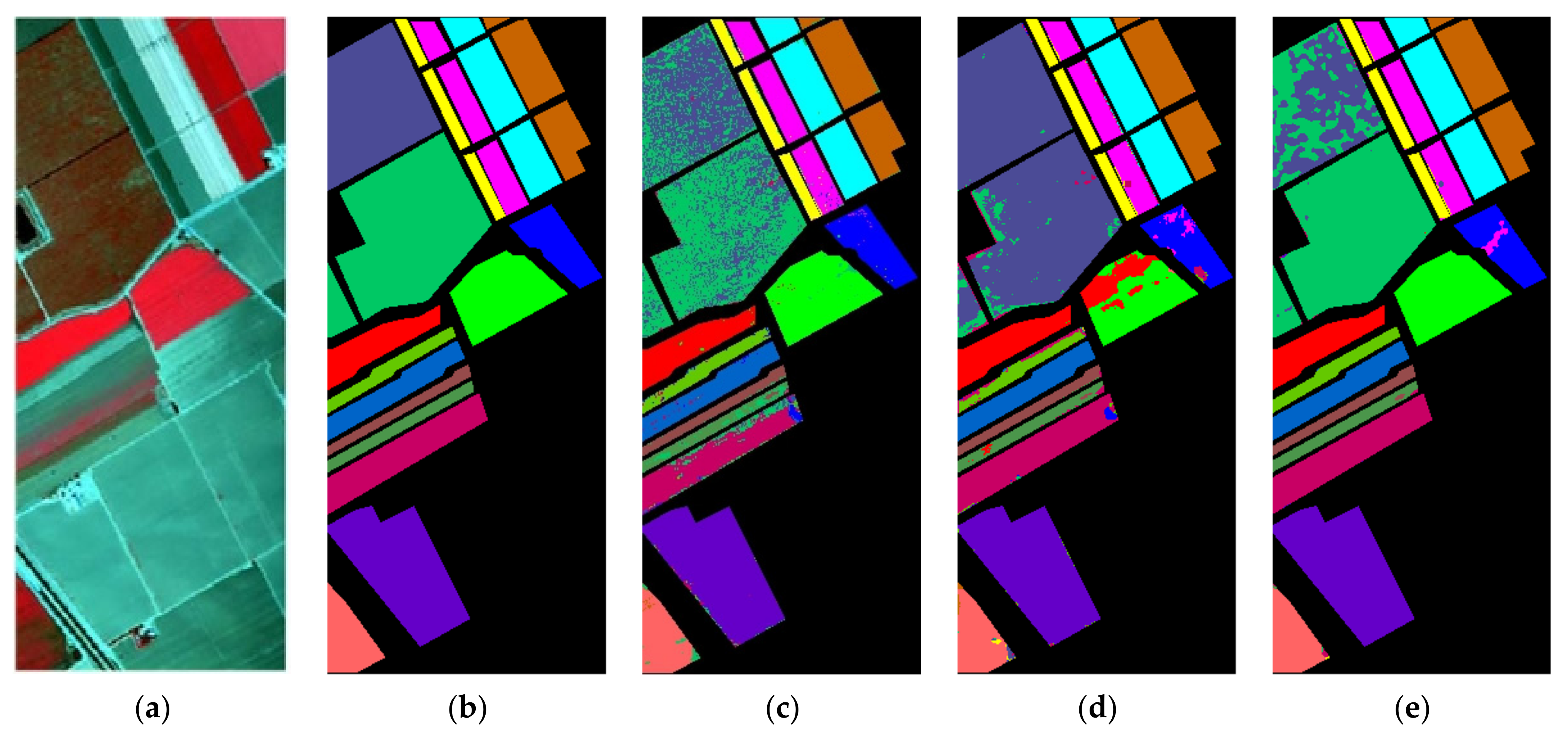
The qualitative classification map can directly reflect the classification results of different methods. Figure 5, Figure 6 and Figure 7 show the classification maps of each compared method.
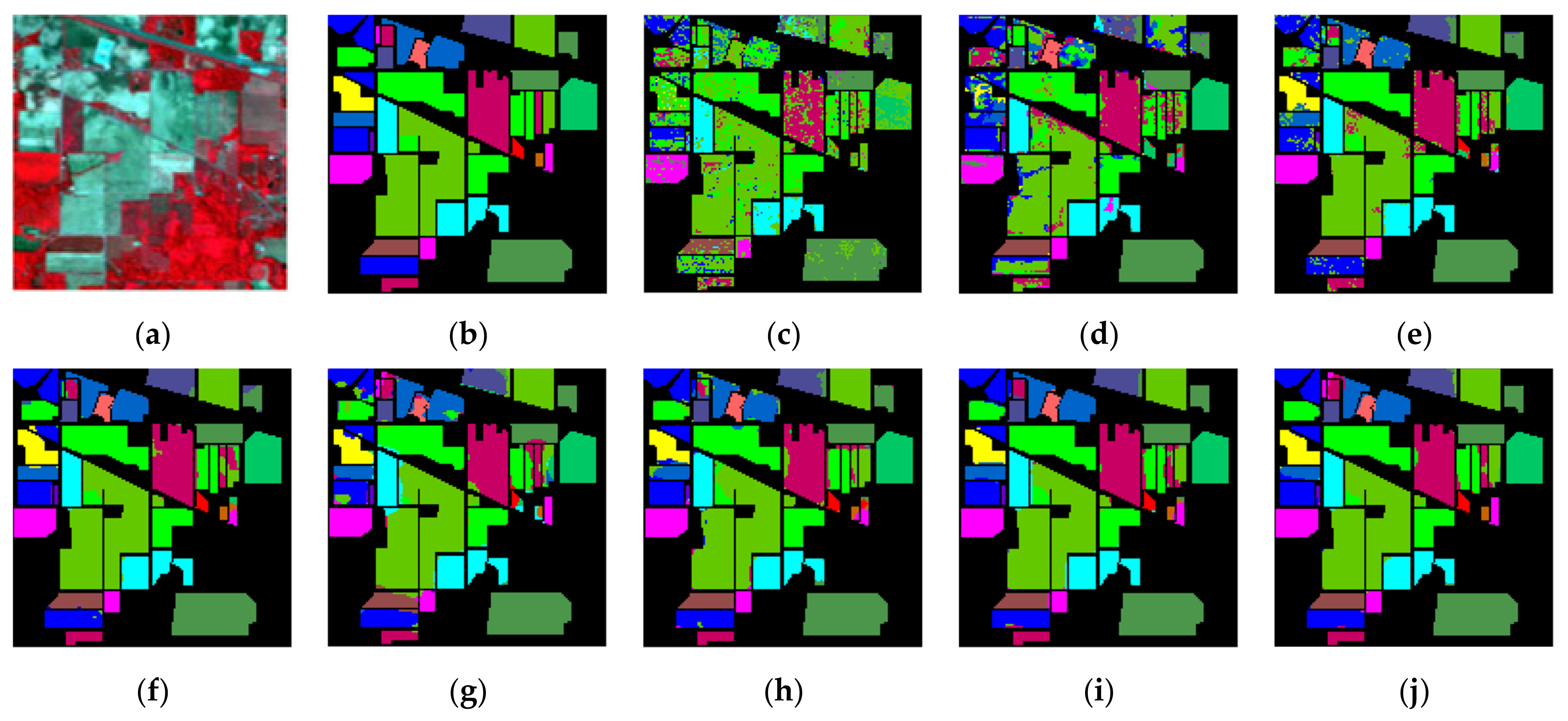
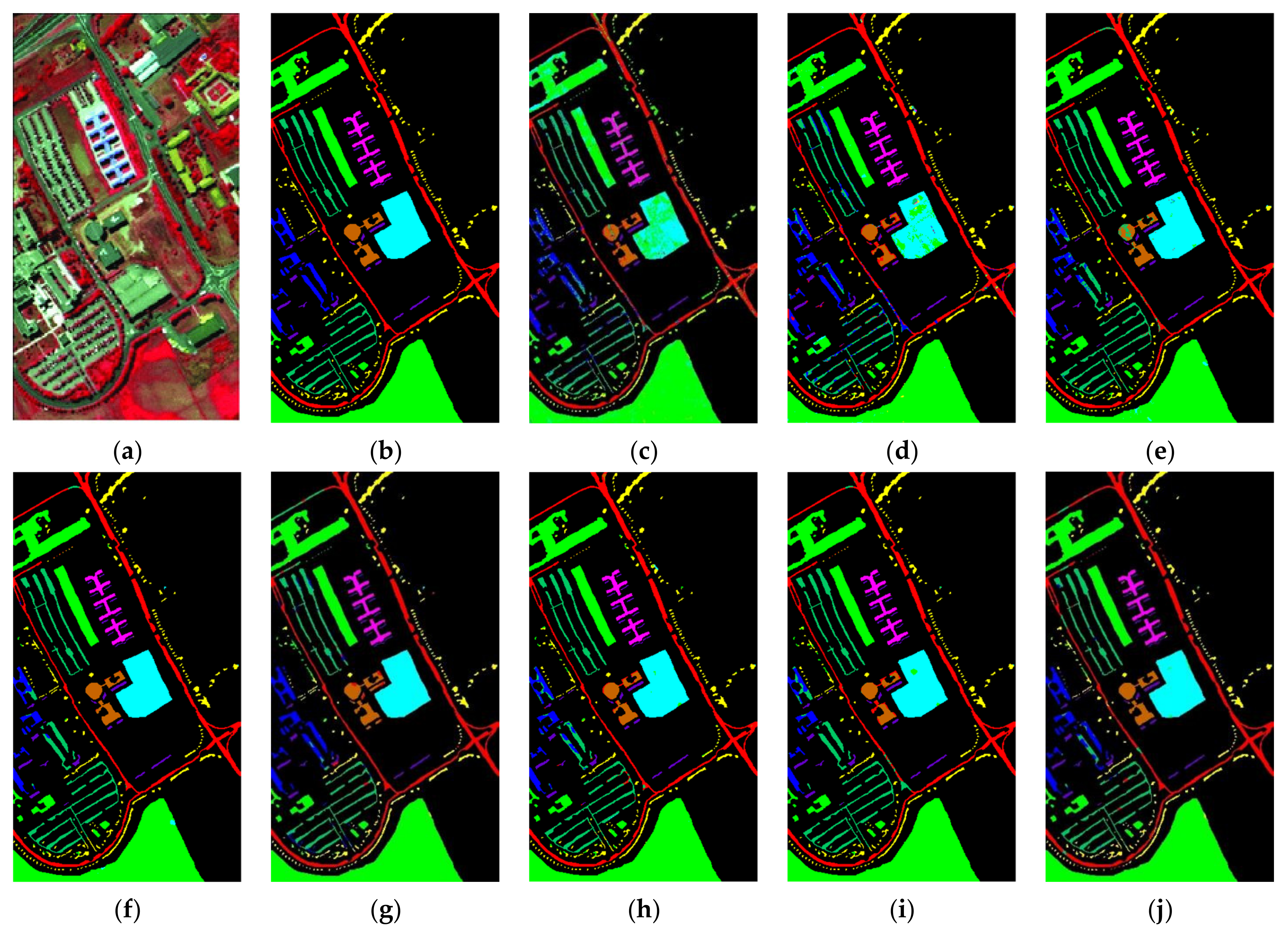
The classification performance of an SVM using only spectral features and CDCNN using only spatial features were found to be the worst. The salt-and-pepper noise was severe, which can be seen in Figure 5c,d, Figure 6c,d and Figure 7c,d. By contrast, the hybrid spectral–spatial features extracted via SSRN, FDSSC, and HybridSN showed better classification performance and less noise in the classification maps. After adding attention mechanisms, the noise of DBMA and DBDA in the IP dataset was very small, whereas the noise in PU and SA was more than that of SSRN, FDSSC, and HybridSN. The hybrid features extracted via the proposed method showed strong robustness and discrimination. In the three datasets, the proposed method achieved the best classification accuracy and relatively clean classification maps.
4.5. Comparison of Different Methods When Different Training Samples Are Considered
To further compare the proposed method with the related methods, the performance of different methods with different numbers of training data was compared. In the three datasets, 1%, 3%, 5%, 10%, and 15% of data were adopted for training. The experimental results are shown in Figure 8.
When 1% of the data were used for training, only the classification accuracy of FDSSC on IP was slightly higher than that of the proposed method. In other cases, the proposed method achieved the best classification performance. With the increase in the training data, the classification performance of the proposed method was better than that of all the compared methods. In summary, the hybrid features extracted by the proposed method have strong discrimination and robustness, and can distinguish well between different categories of pixels.
4.6. Comparison of OA for Different Spatial Sizes
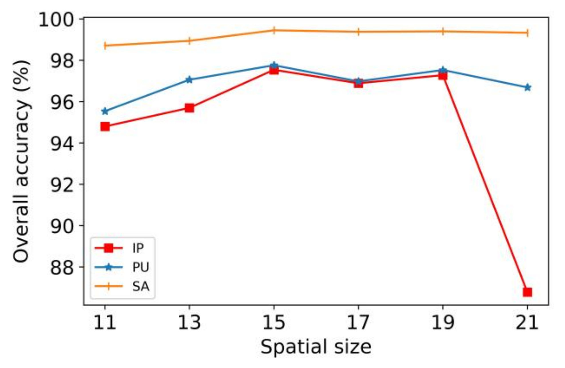
When the spatial size of the selected data cubes is small, it will lead to a lack of spatial information. The extracted features are not sufficient to distinguish different categories of pixels, resulting in lower classification accuracy. If the spatial size is too large, the data cubes will contain more neighborhood pixels, which are likely to contain many other categories of pixels. In other words, the introduction of too much interference data will also lead to low classification accuracy. Therefore, it is very important to select the appropriate spatial size. In this section, we test data cubes of different spatial size from 11 × 11 to 21 × 21, including a total of six cases. The results are shown in Figure 9.
In the tests of the three datasets, the OA of the model increased first and then decreased with the gradual increase in the spatial size. Among these, the fluctuations of PU and SA were small, and the classification performance of IP decreased significantly when the spatial size of IP increased from 19 to 21. This shows that the IP dataset was most affected by the neighborhood pixels. According to the overall optimal classification accuracy, we determined that the spatial size of the data cubes was 15 × 15. Please note that the above analysis is only limited to the proposed method.
4.7. Comparison of OA for Different Learning Rates
As an important hyperparameter in deep learning, the learning rate determines whether and when the objective function converges to the local minimum value. If the learning rate is too large, the loss function may directly exceed the global optimum point. If it is too small, the change rate of the loss function is very slow, which will greatly increase the convergence complexity of the network and easily fall into the local minimum or saddle point. Therefore, the appropriate learning rate makes the objective function converge to the local minimum value at an appropriate time. In this section of our analysis, the learning rate was set to 0.0001, 0.0005, 0.001, and 0.005 for the experiment, respectively, and the results are shown in Figure 10.
As can be seen in Figure 10, when the learning rate increased from 0.0001 to 0.0005, the classification accuracy for IP, PU, and SA increased, respectively. As the learning rate continued to increase, the classification performance showed a continuous downward trend. In addition, during the experiment, when the learning rate was set to 0.0005, the model was able to converge within 80 epochs. When the learning rate was set to 0.0001, the model needed to be trained for more epochs. When the initial learning rate was set to 0.001 and 0.005, the model did not converge to the optimal value. Therefore, 0.0005 was selected as the optimal learning rate of the model.
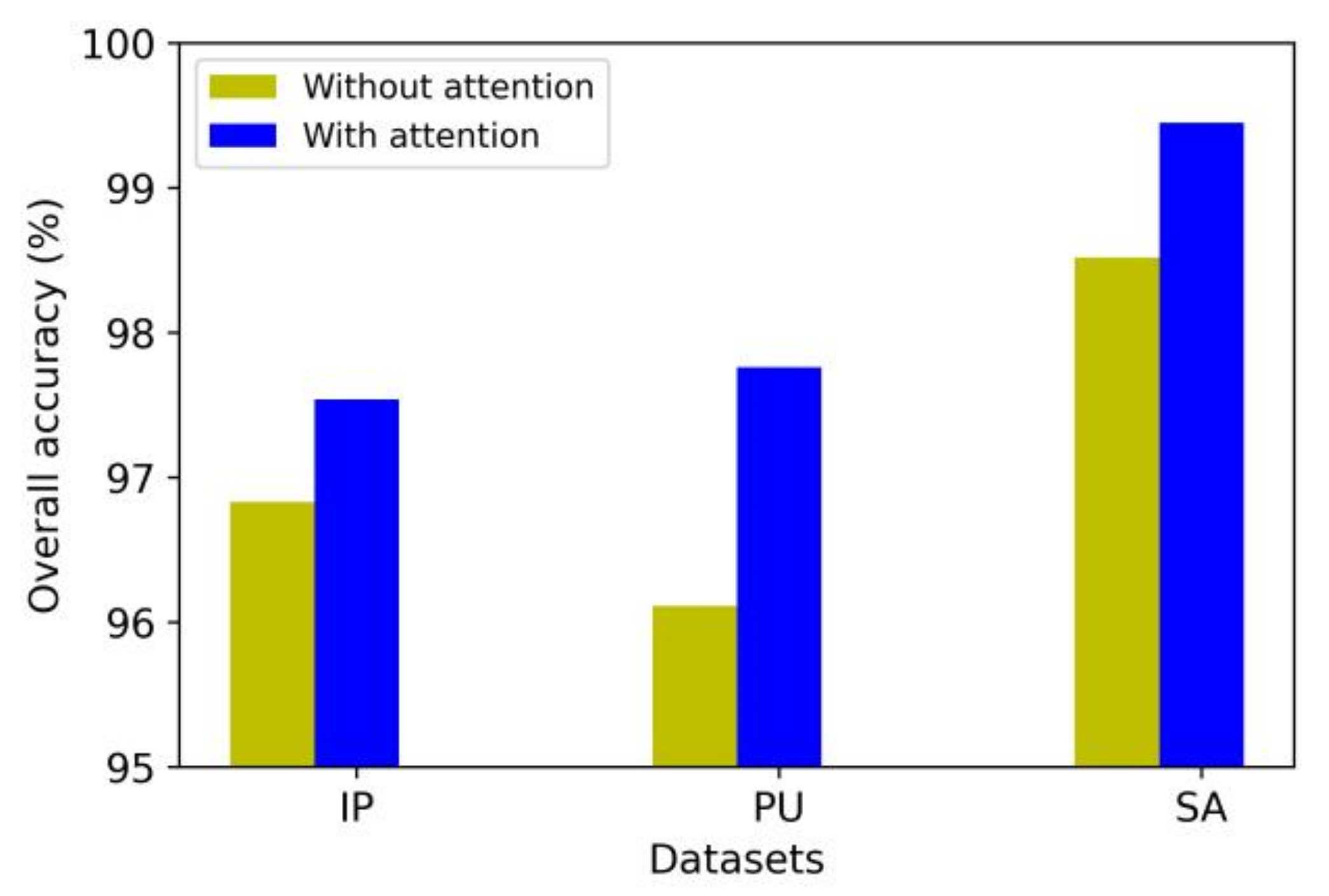
4.8. Analysis of the Attention Mechanism’s Effectiveness
In the proposed method, the original HSI is weighted through the hybrid attention mechanism after the PCA dimension reduction. This module is learnable and can complete both spectral and spatial attention processes simultaneously. In this section, we compare the classification performance of the model with and without the attention mechanism.
As shown in Figure 11, the classification accuracy of the model in three datasets increases to a certain extent after the hybrid attention mechanism is adopted. The experimental results indicate that the proposed hybrid attention mechanism is effective and can further improve the classification performance based on the existing model. In addition, this attention mechanism only uses two small convolution kernels for learning and completes the attention weighting process through two-matrix multiplication and one-matrix addition. Therefore, the proposed attention mechanism consumes very few computational resources.
4.9. The Effectiveness of the Multiscale Method
The two network branches of the proposed model first extract the multiscale spectral and spatial features of the HSI, respectively. Ablation experiments were performed to compare the classification performance of the method with no multiscale feature extraction module, with one multiscale feature extraction module, and with both spectral and spatial multiscale feature extraction modules. The classification performance is shown in Figure 12, where A represents the multiscale spectral feature extraction module, and B represents the multiscale spatial feature extraction module.
As shown in Figure 12, the classification performance of the model was improved to a certain extent after the multiscale spectral feature extraction module or multiscale spatial feature extraction module was adopted. When both modules were used, the classification performance of the model was significantly improved. Therefore, with the introduction of multiscale feature extraction modules, the network can obtain different receptive fields in both spectral and spatial aspects, capture information at different scales, and extract abundant features. The extracted features distinguish between different categories of pixels well and achieve a great improvement in performance in the classification task.
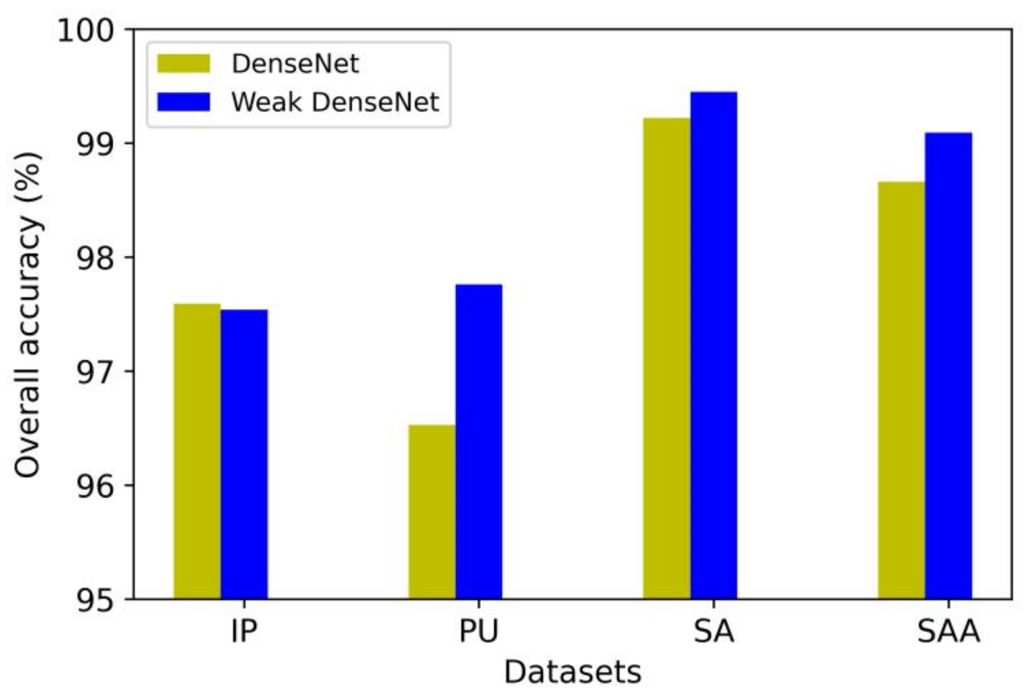
4.10. The Comparison of DenseNet and Weak DenseNet
The weak dense spectral and spatial feature extraction modules used in the proposed method are simplified from the DenseNet model. Only the skip connections between the input and output of each layer based on the DenseNet model are reserved. In this section, we added another dataset, SalinasA (SAA), to train with 1% of the data for more effective comparison. The description of the dataset is as follows:
The SalinasA (SAA) was obtained through the AVIRIS sensor in the Salinas Valley in California, USA. The dataset contains six categories with the size of 83 × 86 pixels. This scene can be corrected by removing 20 water absorption bands (108–112, 154–167, and 224) from 224 spectral bands.
We tested the classification performance of the model by using a weak dense structure and dense structure on the four datasets; the experiment results are shown in Figure 13.
As shown in Figure 13, when the overall network model remained unchanged, the classification performance of the model using the weak dense structure was 0.05% lower than that using a dense structure on IP. For PU and SA, the classification accuracy of the model with a weak dense structure was increased by 1.23% and 0.23%. In order to make the experimental results more convincing, we also tested the SAA dataset. In the proposed method, the use of the weak dense structure showed a 0.43% performance improvement compared to the dense structure in the SAA dataset. Therefore, compared with the dense structure, the weak dense structure can reduce the amount of feature maps with almost no reduction in classification accuracy.
4.11. The Comparison of Averagepooling and Flatten at the End of the Model
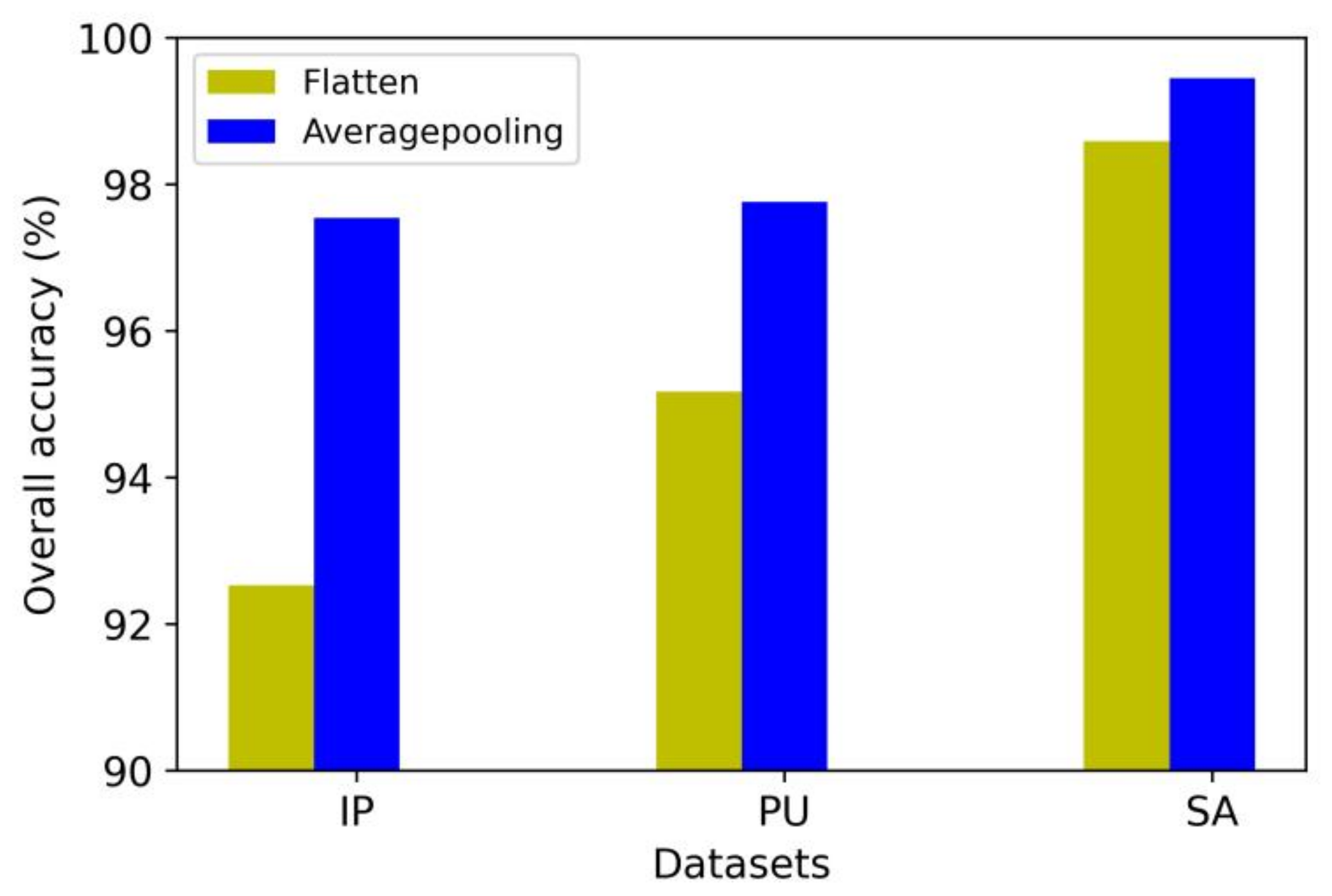
In the proposed method, the high-dimensional spectral and spatial features are first extracted by two network branches. Then, the features are compressed into one dimension by AveragePooling3D. Finally, the features are fed into fully connected layers and a Softmax layer for the classification of the results. There are a number of related methods that directly flatten the high-dimensional features to one dimension and obtain classification results through fully connected layers and a Softmax layer [22,39,40]. Here, we conducted an experimental comparison of the above two approaches; the results are shown in Figure 14.
As can be seen in Figure 14, compared with the AveragePooling3D approach, the classification performance using the flatten method decreased significantly in the three datasets, by 5.01%, 2.59%, and 0.86%, respectively. On the one hand, AveragePooling3D refines the features of each part and retains the most important information. On the other hand, this method can effectively reduce the number of parameters and largely suppress overfitting. Therefore, the proposed method using AveragePooling3D is superior to the flatten method.
4.12. Investigation on Running Time
The training and test time are significant indicators to measure the performance of the model. An excellent classification model depends not only on high classification accuracy but also on a high level of timeliness. Therefore, we compared the training and test times of the model. The comparison results are shown in Table 11, Table 12 and Table 13:
As shown in Table 11, Table 12 and Table 13, compared with SSRN, FDSSC, DBMA, and DBDA, the proposed method has advantages in the training and test time. In addition to the multiscale spatial feature extraction module, the proposed model mostly adopts a CNN with a small kernel scale, especially the 1 × 1 × n convolution kernel in the spectral feature extraction branch. The proposed model has fewer parameters, a fast convergence speed, and high operational efficiency. It is worth noting that the network structure of CDCNN and HybridSN is simple, and the number of parameters is small. The training and test times of the two methods are shorter than those for the proposed method, but their classification accuracy is relatively low.
5. Conclusions
In this paper, a spectral and spatial feature extraction method combined with an attention mechanism is proposed for HSI classification. Firstly, PCA is used to reduce the dimensions of the original HSI, and the hybrid spectral–spatial attention mechanism is adopted to weight the data. This process not only reduces the amount of data and redundant information but also enhances the effectiveness of the data. Then, two network branches composed of multiscale feature extraction modules and weak dense feature extraction modules are used in parallel to extract high-dimensional semantic features of the image. Finally, the AveragePooling3D is adapted to compress the two parts of features, and the classification results are obtained through fully connected layers and a Softmax layer. The hybrid spectral–spatial attention mechanism effectively improves the classification performance of the model, with a learning ability and a very small computational overhead. The compound multiscale weak dense network model has a fast convergence speed, a high efficiency of feature extraction, strong robustness and discrimination of features, and good generalization ability. The experimental results on the three datasets showed that the proposed method is superior to the compared methods in terms of classification accuracy and timeliness.
The shortcoming of the proposed method is that there are too many training parameters in the fully connected layers of the model, which reduces the efficiency of the training and the test stage to a certain extent. In addition, the attention mechanism can improve the classification performance, but the effect is not significant enough. Therefore, our next research goal is still to focus on a network model based on the attention mechanism, to explore a more efficient attention mechanism based on preprocessing or postprocessing, and to improve the classification performance more obviously.
Author Contributions
Conceptualization, Z.G.; methodology, Z.G.; validation, Z.G.; formal analysis, Z.G.; writing—original draft preparation, Z.G.; writing—review and editing, G.C., H.S., Y.Z. and X.L.; funding acquisition, G.C., P.F. and Y.Z. All authors have read and agreed to the published version of the manuscript.
Funding
This work was supported in part by the National Natural Science Foundation of China under Grant 61801222, in part by the Nature Science Foundation of Jiangsu Province under Grant BK20191284 and in part by the Start Foundation of Nanjing University of Posts and Telecommunications (NUPTSF) under Grant NY220157.
Institutional Review Board Statement
Not applicable.
Informed Consent Statement
Not applicable.
Data Availability Statement
Publicly available datasets are analyzed in this study, which can be found here: http://www.ehu.eus/ccwintco/index.php/Hyperspectral_Remote_Sensing_Scenes (accessed on 21 May 2021).
Acknowledgments
The authors would like to thank the editors and reviewers for their insightful suggestions.
Conflicts of Interest
The authors declare no conflict of interest.
References
- Xu, S.; Li, J.; Khodadadzadeh, M.; Marinoni, A.; Gamba, P.; Li, B. Abundance-indicated subspace for hyperspectral classifification with limited training samples. IEEE J. Sel. Top. Appl. Earth Obs. Remote Sens. 2019, 12, 1265–1278. [Google Scholar] [CrossRef]
- Zhang, M.; Li, W.; Du, Q. Diverse region-based CNN for hyperspectral image classifification. IEEE Trans. Image Process. 2018, 27, 2623–2634. [Google Scholar] [CrossRef] [PubMed]
- Garaba, S.P.; Aitken, J.; Slat, B.; Dierssen, H.M.; Lebreton, L.; Zielinski, O.; Reisser, J. Sensing ocean plastics with an airborne hyperspectral shortwave infrared imager. Environ. Sci. Technol. 2018, 52, 11699–11707. [Google Scholar] [CrossRef] [PubMed]
- Ibrahim, A.; Franz, B.; Ahmad, Z.; Healy, R.; Knobelspiesse, K.; Gao, B.; Proctor, C.; Zhai, P. Atmospheric correction for hyperspectral ocean color retrieval with application to the Hyperspectral Imager for the Coastal Ocean (HICO). Remote Sens. Environ. 2018, 204, 60–75. [Google Scholar] [CrossRef] [Green Version]
- Carrino, T.A.; Crósta, A.P.; Toledo, C.L.; Silva, A.M. Hyperspectral remote sensing applied to mineral exploration in southern peru: A multiple data integration approach in the Chapi Chiara gold prospect. Int. J. Appl. Earth Obs. Geoinf. 2018, 64, 287–300. [Google Scholar] [CrossRef]
- Lorenz, S.; Salehi, S.; Kirsch, M.; Zimmermann, R.; Unger, G.; Sørensen, E.V.; Gloaguen, R. Radiometric correction and 3D integration of longrange ground-based hyperspectral imagery for mineral exploration of vertical outcrops. Remote Sens. 2018, 10, 176. [Google Scholar] [CrossRef] [Green Version]
- Shi, Q.; Liu, X.; Li, X. Road detection from remote sensing images by generative adversarial networks. IEEE Access 2017, 6, 25486–25494. [Google Scholar] [CrossRef]
- Wang, F.; Gao, J.; Zha, Y. Hyperspectral sensing of heavy metals in soil and vegetation: Feasibility and challenges. ISPRS J. Photogramm. Remote Sens. 2018, 136, 73–84. [Google Scholar] [CrossRef]
- Lassalle, G.; Credoz, A.; Hédacq, R.; Fabre, S.; Dubucq, D.; Elger, A. Assessing soil contamination due to oil and gas production using vegetation hyperspectral reflectance. Environ. Sci. Technol. 2018, 52, 1756–1764. [Google Scholar] [CrossRef]
- Ke, C. Military Object Detection Using Multiple Information Extracted from Hyperspectral Imagery. In Proceedings of the 2017 International Conference on Progress in Informatics and Computing (PIC), Nanjing, China, 15–17 May 2017; pp. 124–128. [Google Scholar] [CrossRef]
- Shimoni, M.; Haelterman, R.; Perneel, C. Hypersectral imaging for military and security applications: Combining myriad processing and sensing techniques. IEEE Geosci. Remote Sens. Mag. 2019, 7, 101–117. [Google Scholar] [CrossRef]
- Jia, S.; Jiang, S.; Lin, Z.; Xu, M.; Yu, S. A survey: Deep learning for hyperspectral image classification with few labeled samples. Neurocomputing 2021, 448, 179–204. [Google Scholar] [CrossRef]
- Yuan, Y.; Wang, C.; Jiang, Z. Proxy-Based Deep Learning Framework for Spectral-Spatial Hyperspectral Image Classification: Efficient and Robust. IEEE Trans. Geosci. Remote Sens. 2021, 1–15. [Google Scholar] [CrossRef]
- Shen, Y.; Zhu, S.; Chen, C.; Du, Q.; Xiao, L.; Chen, J.; Pan, D. Efficient deep learning of nonlocal features for hyperspectral image classification. IEEE Trans. Geosci. Remote Sens. 2020, 59, 6029–6043. [Google Scholar] [CrossRef]
- Wang, Z.; Chen, J.; Hoi, C. Deep Learning for Image Super-resolution: A Survey. IEEE Trans. Pattern Anal. Mach. Intell. 2020. [Google Scholar] [CrossRef] [Green Version]
- Minaee, M.; Boykov, Y.Y.; Porikli, F.; Plaza, A.J.; Kehtarnavaz, N.; Terzopoulos, D. Image Segmentation Using Deep Learning: A Survey. IEEE Trans. Pattern Anal. Mach. Intell. 2021. [Google Scholar] [CrossRef]
- Haeb-Umbach, R.; Watanabe, S.; Nakatani, T.; Bacchiani, M.; Hoffmeister, B.; Seltzer, M.; Zen, H.; Souden, M. Speech Processing for Digital Home Assistants: Combining Signal Processing With Deep-Learning Techniques. IEEE Signal Process. Mag. 2019, 36, 111–124. [Google Scholar] [CrossRef]
- Alshemali, B.; Kalita, J. Improving the reliability of deep neural networks in NLP: A review. Knowl.-Based Syst. 2020, 191, 105210. [Google Scholar] [CrossRef]
- Lee, H.; Kwon, H. Going deeper with contextual CNN for hyperspectral image classifification. IEEE Trans. Image Process. 2017, 26, 4843–4855. [Google Scholar] [CrossRef] [Green Version]
- Zhong, Z.; Li, J.; Luo, Z.; Chapman, M.; Weinberger, Q. Spectral-spatial residual network for hyperspectral image classifification: A 3-D deep learning framework. IEEE Trans. Geosci. Remote Sens. 2017, 56, 847–858. [Google Scholar] [CrossRef]
- Wang, W.; Dou, S.; Jiang, Z.; Sun, L. A Fast Dense Spectral-Spatial Convolution Network Framework for Hyperspectral Images Classifification. Remote Sens. 2018, 10, 1068. [Google Scholar] [CrossRef] [Green Version]
- Roy, S.K.; Krishna, K.; Dubey, S.R.; Chaudhuri, B.B. HybridSN: Exploring 3-D–2-D CNN feature hierarchy for hyperspectral image classifification. IEEE Geosci. Remote Sens. Lett. 2020, 17, 277–281. [Google Scholar] [CrossRef] [Green Version]
- Ge, Z.; Cao, G.; Li, X.; Fu, P. Hyperspectral image classifification method based on 2D–3D CNN and multibranch feature fusion. IEEE J. Sel. Top. Appl. Earth Obs. Remote Sens. 2020, 13, 5776–5788. [Google Scholar] [CrossRef]
- Huang, L.; Chen, Y. Dual-path siamese CNN for hyperspectral image classification with limited training samples. IEEE Geosci. Remote Sens. Lett. 2020, 18, 518–522. [Google Scholar] [CrossRef]
- Safari, K.; Prasad, S.; Labate, D. A multiscale deep learning approach for high-resolution hyperspectral image classification. IEEE Geosci. Remote Sens. Lett. 2020, 18, 167–171. [Google Scholar] [CrossRef]
- Praveen, B.; Menon, V. Study of Spatial-Spectral Feature Extraction frameworks with 3D Convolutional Neural Network for Robust Hyperspectral Imagery Classification. IEEE J. Sel. Top. Appl. Earth Obs. Remote Sens. 2020, 14, 1717–1727. [Google Scholar] [CrossRef]
- Meng, Z.; Jiao, L.; Liang, M.; Zhao, F. A Lightweight Spectral-Spatial Convolution Module for Hyperspectral Image Classification. IEEE Geosci. Remote Sens. Lett. 2021, 1–5. [Google Scholar] [CrossRef]
- Gao, H.; Chen, Z.; Li, C. Sandwich Convolutional Neural Network for Hyperspectral Image Classification Using Spectral Feature Enhancement. IEEE J. Sel. Top. Appl. Earth Obs. Remote Sens. 2021, 14, 3006–3015. [Google Scholar] [CrossRef]
- Xu, K.; Ba, J.; Kiros, R.; Cho, K.; Courville, A.; Salakhudinov, R.; Zemel, R.; Bengio, Y. Show, Attend and Tell: Neural Image Caption Generation with Visual Attention. In Proceedings of the 32nd International Conference on Machine Learning (PMLR), Lille, France, 7–9 July 2015; pp. 2048–2057. [Google Scholar]
- Fukui, H.; Hirakawa, T.; Yamashita, T.; Fujiyoshi, H. Attention Branch Network: Learning of Attention Mechanism for Visual Explanation. In Proceedings of the 2019 IEEE Conference on Computer Vision and Pattern Recognition (CVPR), Long Beach, CA, USA, 15–20 June 2019; pp. 10705–10714. [Google Scholar] [CrossRef] [Green Version]
- Song, J.; Zeng, P.; Gao, L.; Shen, H. From Pixels to Objects: Cubic Visual Attention for Visual Question Answering. In Proceedings of the 27 International Joint Conference on Artificial Intelligence (IJCAI), Stockholm, Sweden, 13–19 July 2018; pp. 906–912. [Google Scholar]
- Mou, L.; Zhu, X. Learning to pay attention on spectral domain: A spectral attention module-based convolutional network for hyperspectral image classifification. IEEE Trans. Geosci. Remote Sens. 2020, 58, 110–122. [Google Scholar] [CrossRef]
- Mei, X.; Pan, E.; Ma, Y.; Dai, X.; Huang, J.; Fan, F.; Du, Q.; Zheng, H.; Ma, J. Spectral–spatial attention networks for hyperspectral image classifification. Remote Sens. 2019, 11, 963. [Google Scholar] [CrossRef] [Green Version]
- Ge, Z.; Cao, G.; Zhang, Y.; Li, X.; Shi, H.; Fu, P. Adaptive Hash Attention and Lower Triangular Network for Hyperspectral Image Classification. IEEE Trans. Geosci. Remote Sens. 2021, 1–19. [Google Scholar] [CrossRef]
- Yu, C.; Han, R.; Song, M.; Liu, C.; Chang, C. Feedback Attention-Based Dense CNN for Hyperspectral Image Classification. IEEE Trans. Geosci. Remote Sens. 2021, 1–16. [Google Scholar] [CrossRef]
- Zhu, M.; Jiao, L.; Liu, F.; Yang, S.; Wang, J. Residual Spectral-Spatial Attention Network for Hyperspectral Image Classification. IEEE Trans. Geosci. Remote Sens. 2020, 59, 449–462. [Google Scholar] [CrossRef]
- Lin, J.; Mou, L.; Zhu, X.; Ji, X.; Wang, Z.J. Attention-Aware Pseudo-3-D Convolutional Neural Network for Hyperspectral Image Classification. IEEE Trans. Geosci. Remote Sens. 2021, 1–13. [Google Scholar] [CrossRef]
- Guo, W.; Ye, H.; Cao, F. Feature-Grouped Network With Spectral-Spatial Connected Attention for Hyperspectral Image Classification. IEEE Trans. Geosci. Remote Sens. 2021, 1–13. [Google Scholar] [CrossRef]
- Ma, W.; Yang, Q.; Wu, Y.; Zhao, W.; Zhang, X. Double-branch multi-attention mechanism network for hyperspectral image classifification. Remote Sens. 2019, 11, 1307. [Google Scholar] [CrossRef] [Green Version]
- Li, R.; Zheng, S.; Duan, C.; Yang, Y.; Wang, X. Classifification of hyperspectral image based on double-branch dual-attention mechanism network. Remote Sens. 2020, 12, 582. [Google Scholar] [CrossRef] [Green Version]
- Tang, X.; Meng, F.; Zhang, X.; Cheung, Y.; Liu, F.; Jiao, L. Hyperspectral Image Classification Based on 3-D Octave Convolution With Spatial-Spectral Attention Network. IEEE Trans. Geosci. Remote Sens. 2020, 59, 2430–2447. [Google Scholar] [CrossRef]
- Xue, Z.; Zhang, M.; Liu, Y.; Du, P. Attention-Based Second-Order Pooling Network for Hyperspectral Image Classification. IEEE Trans. Geosci. Remote Sens. 2021, 1–16. [Google Scholar] [CrossRef]
- Zhang, Z.; Liu, D.; Gao, D.; Shi, G. S3Net: Spectral-Spatial-Semantic Network for Hyperspectral Image Classification With the Multiway Attention Mechanism. IEEE Trans. Geosci. Remote Sens. 2021, 1–17. [Google Scholar] [CrossRef]
- Pu, C.; Huang, H.; Luo, L. Classfication of Hyperspectral Image with Attention Mechanism-Based Dual-Path Convolutional Network. IEEE Geosci. Remote Sens. Lett. 2021, 1–5. [Google Scholar] [CrossRef]
- Cui, Y.; Yu, Z.; Han, J.; Gao, S.; Wang, L. Dual-Triple Attention Network for Hyperspectral Image Classification Using Limited Training Samples. IEEE Geosci. Remote Sens. Lett. 2021, 1–5. [Google Scholar] [CrossRef]
- Zhao, Z.; Hu, D.; Wang, H.; Yu, X. Center Attention Network for Hyperspectral Image Classification. IEEE J. Sel. Top. Appl. Earth Obs. Remote Sens. 2021, 14, 3415–3425. [Google Scholar] [CrossRef]
- Xue, Z.; Yu, X.; Liu, B.; Tan, X.; Wei, X. HResNetAM: Hierarchical Residual Network with Attention Mechanism for Hyperspectral Image Classification. IEEE J. Sel. Top. Appl. Earth Obs. Remote Sens. 2021, 14, 3566–3580. [Google Scholar] [CrossRef]
- He, K.; Zhang, X.; Ren, S.; Sun, J. Deep Residual Learning for Image Recognition. In Proceedings of the 2016 IEEE Conference on Computer Vision and Pattern Recognition (CVPR), Las Vegas, NV, USA, 27–30 June 2016; pp. 770–778. [Google Scholar] [CrossRef] [Green Version]
- Huang, G.; Liu, Z.; Maaten, L.; Weinberger, K.Q. Densely Connected Convolutional Networks. In Proceedings of the 2017 IEEE Conference on Computer Vision and Pattern Recognition (CVPR), Honolulu, HI, USA, 21–26 July 2017; pp. 4700–4708. [Google Scholar] [CrossRef] [Green Version]
- Galassi, A.; Lippi, M.; Torroni, P. Attention in natural language processing. IEEE Trans. Neural Netw. Learn. Syst. 2020, 1–18. [Google Scholar] [CrossRef] [PubMed]
- Dong, Z.; Wu, T.; Song, S.; Zhang, M. Interactive Attention Model Explorer for Natural Language Processing Tasks with Unbalanced Data Sizes. In Proceedings of the 2020 IEEE Pacific Visualization Symposium (PacificVis), Tianjin, China, 3–5 June 2020; pp. 46–50. [Google Scholar] [CrossRef]
- Chen, Y.; Liu, L.; Phonevilay, V.; Gu, K.; Xia, R.; Xie, J.; Zhang, Q.; Yang, K. Image super-resolution reconstruction based on feature map attention mechanism. Appl. Intell. 2021, 51, 4367–4380. [Google Scholar] [CrossRef]
- Xu, R.; Tao, Y.; Lu, Z.; Zhong, Y. Attention-mechanism-containing neural networks for high-resolution remote sensing image classification. Remote Sens. 2018, 10, 1602. [Google Scholar] [CrossRef] [Green Version]
- Hinton, G.E.; Srivastava, N.; Krizhevsky, A.; Sutskever, I.; Salakhutdinov, R.R. Improving Neural Networks by Preventing Coadaptation of Feature Detectors. arXiv 2012, arXiv:1207.0580. [Google Scholar]
Figure 1.
Flowcharts of ResNet and DenseNet. (a) ResNet, (b) DenseNet.

Figure 2.
Flowchart of the hybrid attention mechanism.
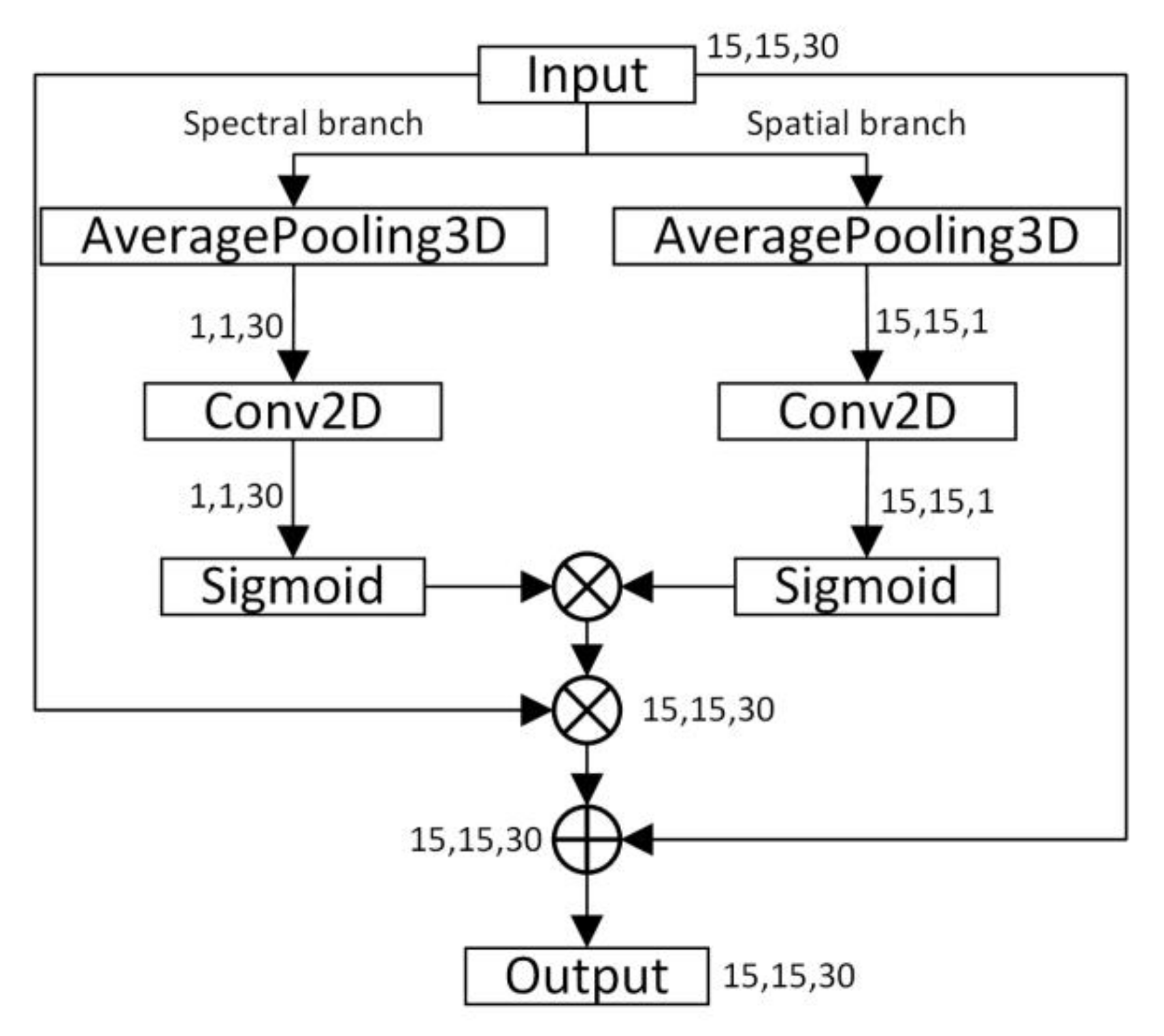
Figure 3.
Flowchart of multiscale feature extraction modules. (a) Multiscale spectral feature extraction module; (b) multiscale spatial feature extraction module.
Figure 3.
Flowchart of multiscale feature extraction modules. (a) Multiscale spectral feature extraction module; (b) multiscale spatial feature extraction module.
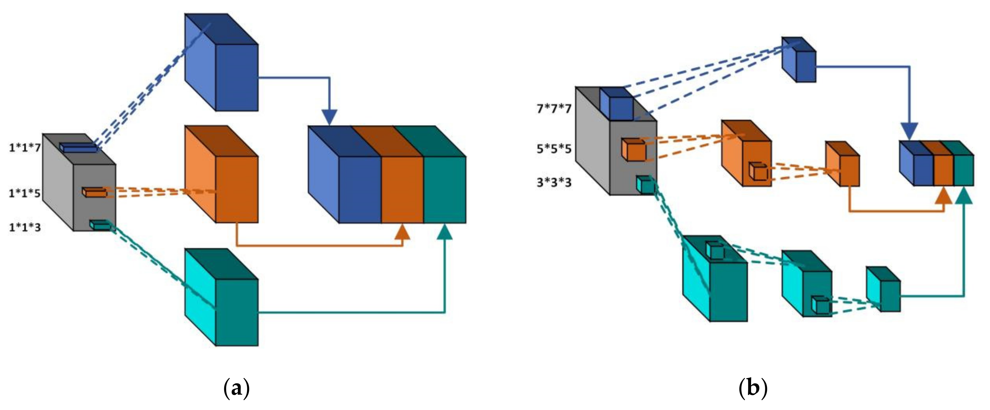
Figure 4.
Overall network structure.

Figure 5.
Classification maps for IP dataset using 5% training samples. (a) False-color image; (b) ground truth; (c) SVM (OA: 68.94%); (d) CDCNN (OA: 76.36%); (e) SSRN (OA: 93.56%); (f) FDSSC (OA: 94.81%); (g) HybridSN (OA: 93.20%); (h) DBMA (OA: 94.46%); (i) DBDA (OA: 97.19%); (j) proposed method (OA: 97.54%).

Figure 6.
Classification maps for PU dataset using 1% training samples. (a) False-color image; (b) ground truth; (c) SVM (OA: 84.71%); (d) CDCNN (OA: 91.88%); (e) SSRN (OA: 97.12%); (f) FDSSC (OA: 97.19%); (g) HybridSN (OA: 96.38%); (h) DBMA (OA: 96.85%); (i) DBDA (OA: 95.87%); (j) proposed method (OA: 97.76%).

Figure 7.
Classification maps for SA dataset using 1% training samples. (a) False-color image; (b) ground truth; (c) SVM (OA: 86.89%); (d) CDCNN (OA: 76.84%); (e) SSRN (OA: 93.43%); (f) FDSSC (OA: 98.52%); (g) HybridSN (OA: 98.33%); (h) DBMA (OA: 95.86%); (i) DBDA (OA: 95.53%); (j) proposed method (OA: 99.45%).


Figure 8.
OA of six methods with different numbers of training samples on (a) IP; (b) PU; (c) SA.

Figure 9.
Performance of the proposed method with different input spatial size.

Figure 10.
Performance of the proposed method with different learning rates.
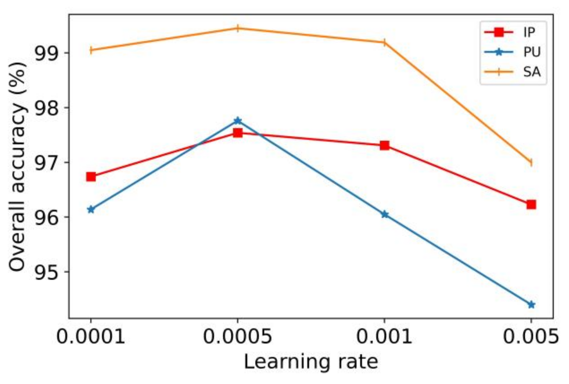
Figure 11.
Effectiveness of the attention mechanism.

Figure 12.
Effectiveness of multiscale mechanisms.
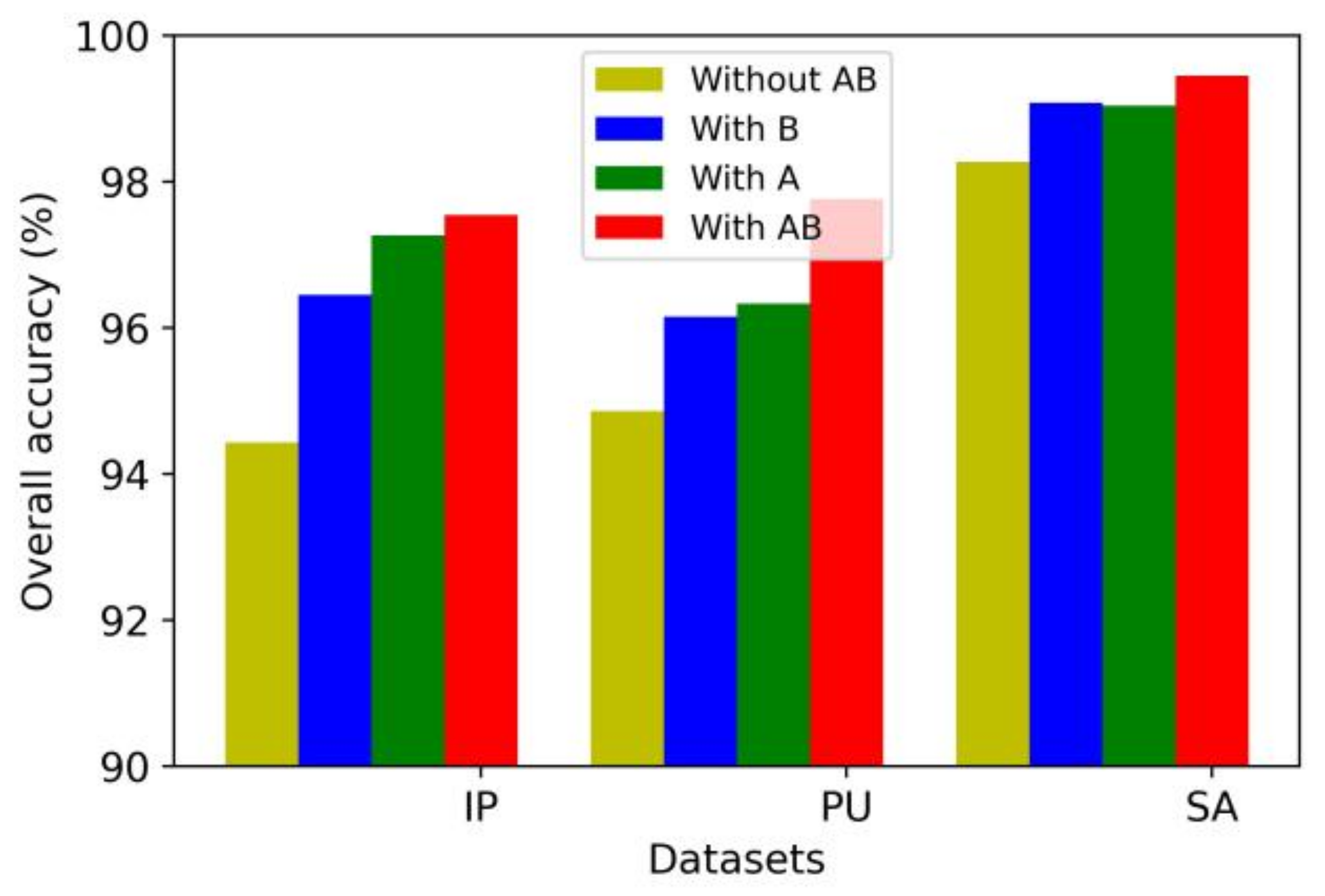
Figure 13.
The comparison of weak DenseNet module and DenseNet module.

Figure 14.
Comparison of AveragePooling and flatten.


Table 1.
The implementation details of the multiscale spectral feature extraction module.
| Module | Layer | Input Shape | Output Shape | Kernel Size | Filters | Connected to |
|---|---|---|---|---|---|---|
| Multiscale spectral feature extraction | Input | - | (15,15,30,1) | - | - | - |
| Conv3d_111 | (15,15,30,1) | (15,15,28,16) | (1,1,3) | 16 | Input | |
| Conv3d_112 | (15,15,30,1) | (15,15,26,16) | (1,1,5) | 16 | Input | |
| Conv3d_113 | (15,15,30,1) | (15,15,24,16) | (1,1,7) | 16 | Input | |
| Fusion11 | (15,15,28,16) (15,15,26,16) (15,15,24,16) | (15,15,78,16) | - | - | Conv3d_111 Conv3d_112 Conv3d_113 | |
| Conv3d_114 | (15,15,78,16) | (9,9,72,16) | (7,7,7) | 16 | Fusion11 |
Table 2.
The implementation details of the multiscale spatial feature extraction module.
| Module | Layer | Input Shape | Output Shape | Kernel Size | Filters | Connected to |
|---|---|---|---|---|---|---|
| Multiscale spatial feature extraction | Input | - | (15,15,30,1) | - | - | - |
| Conv3d_121 | (15,15,30,1) | (9,9,24,16) | (7,7,7) | 16 | Input | |
| Conv3d_1221 | (15,15,30,1) | (11,11,26,8) | (5,5,5) | 8 | Input | |
| Conv3d_1222 | (11,11,26,8) | (9,9,24,16) | (3,3,3) | 16 | Conv3d_1221 | |
| Conv3d_1231 | (15,15,30,1) | (13,13,28,4) | (3,3,3) | 4 | Input | |
| Conv3d_1232 | (13,13,28,4) | (11,11,26,8) | (3,3,3) | 8 | Conv3d_1231 | |
| Conv3d_1233 | (11,11,26,8) | (9,9,24,16) | (3,3,3) | 16 | Conv3d_1232 | |
| Fusion21 | (9,9,24,16) (9,9,24,16) (9,9,24,16) | (9,9,72,16) | - | - | Conv3d_121 Conv3d_1222 Conv3d_1233 | |
| Conv3d_214 | (9,9,72,16) | (9,9,72,16) | (1,1,1) | 16 | Fusion21 |
Table 3.
The implementation details of the spectral weak dense feature extraction module.
| Module | Layer | Input Shape | Output Shape | Kernel Size | Filters | Connected to |
|---|---|---|---|---|---|---|
| Spectral weak dense module | Conv3d_121 | (9,9,72,16) | (9,9,72,16) | (1,1,3) | 16 | Fusion_11 |
| Fusion121 | (9,9,72,16) (9,9,72,16) | (9,9,144,16) | - | - | Conv3d_114 Conv3d_121 | |
| Conv3d_122 | (9,9,144,16) | (9,9,72,16) | (1,1,3) | 16 | Fusion121 | |
| Fusion122 | (9,9,72,16) (9,9,72,16) | (9,9,144,16) | - | - | Conv3d_121 Conv3d_122 | |
| Conv3d_123 | (9,9,144,16) | (9,9,72,16) | (1,1,3) | 16 | Fusion122 | |
| Fusion123 | (9,9,72,16) (9,9,72,16) | (9,9,144,16) | - | - | Conv3d_122 Conv3d_123 |
Table 4.
The implementation details of the spatial weak dense feature extraction module.
| Module | Layer | Input Shape | Output Shape | Kernel Size | Filters | Connected to |
|---|---|---|---|---|---|---|
| Spatial weak dense module | Conv3d_221 | (9,9,72,16) | (9,9,72,16) | (3,3,3) | 16 | Fusion_21 |
| Fusion221 | (9,9,72,16) (9,9,72,16) | (9,9,144,16) | - | - | Conv3d_124 Conv3d_221 | |
| Conv3d_222 | (9,9,144,16) | (9,9,72,16) | (3,3,3) | 16 | Fusion221 | |
| Fusion222 | (9,9,72,16) (9,9,72,16) | (9,9,144,16) | - | - | Conv3d_221 Conv3d_222 | |
| Conv223 | (9,9,144,16) | (9,9,72,16) | (3,3,3) | 16 | Fusion222 | |
| Fusion223 | (9,9,72,16) (9,9,72,16) | (9,9,144,16) | - | - | Conv3d_222 Conv3d_223 |
Table 5.
Land-cover classes and corresponding numbers of samples in the IP dataset.
| No. | Class | Train | Val | Test | Total |
|---|---|---|---|---|---|
| 1 | Alfalfa | 2 | 2 | 42 | 46 |
| 2 | Corn-notill | 71 | 71 | 1286 | 1428 |
| 3 | Corn-mintill | 42 | 42 | 746 | 830 |
| 4 | Corn | 12 | 12 | 213 | 237 |
| 5 | Grass-pasture | 24 | 24 | 435 | 483 |
| 6 | Grass-trees | 36 | 36 | 658 | 730 |
| 7 | Grass-pasture-mowed | 1 | 1 | 26 | 28 |
| 8 | Hay-windrowed | 24 | 24 | 430 | 478 |
| 9 | Oats | 1 | 1 | 18 | 20 |
| 10 | Soybean-notill | 49 | 49 | 874 | 972 |
| 11 | Soybean-mintil | 123 | 123 | 2209 | 2455 |
| 12 | Soybean-clean | 30 | 30 | 533 | 593 |
| 13 | Wheat | 10 | 10 | 185 | 205 |
| 14 | Woods | 63 | 63 | 1139 | 1265 |
| 15 | Buildings-Grass-Trees-Drives | 19 | 19 | 348 | 386 |
| 16 | Stone-Steel-Towers | 5 | 5 | 83 | 93 |
| Total | 512 | 512 | 9225 | 10,249 |
Table 6.
Land-cover classes and corresponding numbers of samples in the PU dataset.
| No. | Class | Train | Val | Test | Total |
|---|---|---|---|---|---|
| 1 | Asphalt | 66 | 66 | 6499 | 6631 |
| 2 | Meadows | 186 | 186 | 18,277 | 18,649 |
| 3 | Gravel | 21 | 21 | 2057 | 2099 |
| 4 | Trees | 31 | 31 | 3002 | 3064 |
| 5 | Painted metal sheets | 13 | 13 | 1319 | 1345 |
| 6 | Bare Soil | 50 | 50 | 4929 | 5029 |
| 7 | Bitumen | 13 | 13 | 1304 | 1330 |
| 8 | Self-Blocking Bricks | 37 | 37 | 3608 | 3682 |
| 9 | Shadows | 9 | 9 | 929 | 947 |
| Total | 426 | 426 | 41,924 | 42,776 |
Table 7.
Land-cover classes and corresponding numbers of samples in the SA dataset.
| No. | Class | Train | Val | Test | Total |
|---|---|---|---|---|---|
| 1 | Brocoli-green-weeds-1 | 20 | 20 | 1969 | 2009 |
| 2 | Brocoli-green-weeds-2 | 37 | 37 | 3652 | 3726 |
| 3 | Fallow | 20 | 20 | 1936 | 1976 |
| 4 | Fallow-rough-plow | 14 | 14 | 1366 | 1394 |
| 5 | Fallow-smooth | 27 | 27 | 2624 | 2678 |
| 6 | Stubble | 40 | 40 | 3879 | 3959 |
| 7 | Celery | 36 | 36 | 3507 | 3579 |
| 8 | Grapes-untrained | 113 | 113 | 11,045 | 11,271 |
| 9 | Soil-vinyard-develop | 62 | 62 | 6079 | 6203 |
| 10 | Corn-senesced-green-weeds | 33 | 33 | 3212 | 3278 |
| 11 | Lettuce-romaine-4wk | 11 | 11 | 1046 | 1068 |
| 12 | Lettuce-romaine-5wk | 19 | 19 | 1889 | 1927 |
| 13 | Lettuce-romaine-6wk | 9 | 9 | 898 | 916 |
| 14 | Lettuce-romaine-7wk | 11 | 11 | 1048 | 1070 |
| 15 | Vinyard-untrained | 73 | 73 | 7122 | 7268 |
| 16 | Vinyard-vertical-trellis | 18 | 18 | 1771 | 1807 |
| Total | 543 | 543 | 53,043 | 54,129 |
Table 8.
The classification accuracy of different methods for the IP dataset.
| Class | SVM | CDCNN | SSRN | FDSSC | HybridSN | DBMA | DBDA | Proposed |
|---|---|---|---|---|---|---|---|---|
| 1 | 10.87 | 0 | 86.67 | 96.51 | 85.29 | 75.93 | 100 | 97.78 |
| 2 | 66.74 | 71.98 | 96.99 | 87.84 | 96.69 | 95.89 | 98.46 | 98.26 |
| 3 | 45.90 | 53.34 | 99.11 | 95.96 | 83.45 | 93.22 | 95.89 | 95.72 |
| 4 | 8.02 | 73.21 | 97.00 | 96.26 | 94.48 | 100 | 99.51 | 99.55 |
| 5 | 69.15 | 87.56 | 99.01 | 99.28 | 81.02 | 95.48 | 96.73 | 97.02 |
| 6 | 90.68 | 94.52 | 98.33 | 98.65 | 89.18 | 99.22 | 94.36 | 99.41 |
| 7 | 17.86 | 25.00 | 86.96 | 84.29 | 100 | 69.57 | 80.00 | 100 |
| 8 | 50.63 | 84.36 | 96.01 | 98.33 | 100 | 100 | 100 | 98.48 |
| 9 | 30.00 | 93.33 | 66.67 | 80.77 | 85.00 | 76.92 | 100 | 100 |
| 10 | 62.35 | 62.67 | 82.55 | 89.94 | 92.61 | 93.64 | 93.68 | 95.69 |
| 11 | 83.30 | 78.13 | 90.89 | 97.79 | 94.44 | 91.56 | 99.03 | 96.73 |
| 12 | 23.78 | 50.36 | 92.02 | 97.49 | 92.93 | 92.84 | 97.03 | 97.51 |
| 13 | 79.51 | 84.33 | 100 | 100 | 95.45 | 100 | 100 | 98.99 |
| 14 | 90.28 | 91.83 | 94.87 | 96.39 | 99.83 | 95.05 | 96.60 | 98.85 |
| 15 | 12.18 | 91.46 | 95.24 | 93.98 | 91.82 | 95.45 | 95.89 | 99.13 |
| 16 | 7.53 | 92.31 | 98.82 | 97.08 | 89.19 | 97.67 | 98.81 | 93.75 |
| OA | 68.94 | 76.36 | 93.56 | 94.81 | 93.20 | 94.46 | 97.19 | 97.54 |
| AA | 46.80 | 70.90 | 92.57 | 94.41 | 91.96 | 92.03 | 96.62 | 97.93 |
| Kappa | 59.63 | 72.97 | 92.65 | 94.10 | 92.24 | 93.67 | 96.80 | 97.19 |
Table 9.
The classification accuracy of different methods for the PU dataset.
| Class | SVM | CDCNN | SSRN | FDSSC | HybridSN | DBMA | DBDA | Proposed |
|---|---|---|---|---|---|---|---|---|
| 1 | 84.65 | 90.21 | 98.90 | 99.44 | 95.76 | 96.50 | 96.07 | 98.29 |
| 2 | 92.57 | 94.66 | 98.23 | 99.45 | 98.73 | 98.72 | 98.86 | 99.34 |
| 3 | 74.94 | 64.95 | 98.93 | 99.52 | 85.03 | 100 | 100 | 96.34 |
| 4 | 70.53 | 97.24 | 99.64 | 97.61 | 97.83 | 97.85 | 98.74 | 96.70 |
| 5 | 90.19 | 98.36 | 99.70 | 99.70 | 99.70 | 99.25 | 100 | 98.66 |
| 6 | 66.41 | 93.11 | 98.62 | 98.50 | 99.82 | 99.15 | 99.88 | 99.98 |
| 7 | 78.87 | 96.88 | 94.25 | 100 | 89.09 | 96.97 | 99.25 | 98.87 |
| 8 | 83.84 | 88.98 | 84.91 | 80.08 | 88.47 | 83.23 | 74.81 | 87.68 |
| 9 | 98.94 | 99.17 | 99.78 | 99.89 | 98.62 | 100 | 99.67 | 97.45 |
| OA | 84.71 | 91.88 | 97.12 | 97.19 | 96.38 | 96.85 | 95.87 | 97.76 |
| AA | 82.33 | 91.51 | 96.99 | 97.13 | 94.78 | 96.85 | 96.36 | 97.03 |
| Kappa | 79.45 | 89.15 | 96.17 | 96.27 | 95.19 | 95.81 | 94.51 | 97.03 |
Table 10.
The classification accuracy of different methods for the SA dataset.
| Class | SVM | CDCNN | SSRN | FDSSC | HybridSN | DBMA | DBDA | Proposed |
|---|---|---|---|---|---|---|---|---|
| 1 | 99.10 | 64.11 | 99.95 | 100 | 98.42 | 100 | 100 | 100 |
| 2 | 97.61 | 99.92 | 99.97 | 100 | 99.97 | 99.92 | 100 | 100 |
| 3 | 98.18 | 95.48 | 99.83 | 98.38 | 100 | 100 | 99.34 | 100 |
| 4 | 97.20 | 94.00 | 96.37 | 94.45 | 95.50 | 97.47 | 93.70 | 99.64 |
| 5 | 96.64 | 93.40 | 93.48 | 99.92 | 88.23 | 81.79 | 99.71 | 97.93 |
| 6 | 98.41 | 99.01 | 100 | 99.97 | 100 | 100 | 100 | 100 |
| 7 | 99.16 | 99.07 | 100 | 99.91 | 99.69 | 100 | 99.91 | 100 |
| 8 | 73.29 | 96.75 | 78.06 | 98.40 | 98.77 | 89.38 | 99.06 | 98.69 |
| 9 | 98.21 | 99.84 | 99.77 | 100 | 99.84 | 99.61 | 99.06 | 99.98 |
| 10 | 79.77 | 82.52 | 97.96 | 92.41 | 99.63 | 96.43 | 99.37 | 99.88 |
| 11 | 92.79 | 92.64 | 100 | 100 | 100 | 99.24 | 99.90 | 100 |
| 12 | 97.30 | 99.63 | 99.89 | 100 | 100 | 99.95 | 100 | 100 |
| 13 | 97.27 | 97.56 | 96.87 | 100 | 99.55 | 100 | 99.89 | 100 |
| 14 | 69.81 | 98.85 | 99.41 | 98.48 | 98.78 | 95.74 | 98.86 | 94.28 |
| 15 | 67.47 | 41.64 | 98.82 | 97.31 | 96.38 | 98.06 | 77.38 | 99.74 |
| 16 | 94.19 | 98.87 | 100 | 99.09 | 100 | 99.88 | 100 | 100 |
| OA | 86.89 | 76.84 | 93.43 | 98.52 | 98.33 | 95.86 | 95.53 | 99.45 |
| AA | 91.03 | 90.83 | 97.52 | 98.65 | 98.42 | 97.34 | 97.89 | 99.38 |
| Kappa | 85.37 | 74.63 | 92.65 | 98.36 | 98.15 | 95.38 | 95.04 | 99.38 |
Table 11.
The training time and test time in seconds (s) for different methods on the IP dataset.
| CDCNN | SSRN | FDSSC | HybridSN | DBMA | DBDA | Proposed | |
|---|---|---|---|---|---|---|---|
| Train (s) | 55.62 | 198.03 | 347.15 | 144.42 | 277.34 | 195.92 | 84.95 |
| Test (s) | 3.29 | 5.65 | 5.42 | 2.86 | 9.59 | 5.98 | 4.01 |
Table 12.
The training time and test time in seconds (s) for different methods on the PU dataset.
| CDCNN | SSRN | FDSSC | HybridSN | DBMA | DBDA | Proposed | |
|---|---|---|---|---|---|---|---|
| Train (s) | 39.29 | 102.26 | 209.81 | 33.39 | 104.93 | 122.71 | 85.12 |
| Test (s) | 14.44 | 18.84 | 28.63 | 3.41 | 36.99 | 33.13 | 19.01 |
Table 13.
The training time and test time in seconds (s) for different methods on the SA dataset.
| CDCNN | SSRN | FDSSC | HybridSN | DBMA | DBDA | Proposed | |
|---|---|---|---|---|---|---|---|
| Train (s) | 29.38 | 233.84 | 565.45 | 51.18 | 260.34 | 297.41 | 87.69 |
| Test (s) | 18.26 | 33.16 | 61.56 | 4.77 | 55.85 | 69.81 | 24.88 |
Publisher’s Note: MDPI stays neutral with regard to jurisdictional claims in published maps and institutional affiliations. |
© 2021 by the authors. Licensee MDPI, Basel, Switzerland. This article is an open access article distributed under the terms and conditions of the Creative Commons Attribution (CC BY) license (https://creativecommons.org/licenses/by/4.0/).
Share and Cite
MDPI and ACS Style
Ge, Z.; Cao, G.; Shi, H.; Zhang, Y.; Li, X.; Fu, P. Compound Multiscale Weak Dense Network with Hybrid Attention for Hyperspectral Image Classification. Remote Sens. 2021, 13, 3305. https://0-doi-org.brum.beds.ac.uk/10.3390/rs13163305
AMA Style
Ge Z, Cao G, Shi H, Zhang Y, Li X, Fu P. Compound Multiscale Weak Dense Network with Hybrid Attention for Hyperspectral Image Classification. Remote Sensing. 2021; 13(16):3305. https://0-doi-org.brum.beds.ac.uk/10.3390/rs13163305
Chicago/Turabian StyleGe, Zixian, Guo Cao, Hao Shi, Youqiang Zhang, Xuesong Li, and Peng Fu. 2021. "Compound Multiscale Weak Dense Network with Hybrid Attention for Hyperspectral Image Classification" Remote Sensing 13, no. 16: 3305. https://0-doi-org.brum.beds.ac.uk/10.3390/rs13163305
Note that from the first issue of 2016, this journal uses article numbers instead of page numbers. See further details here.