
Multi-Stage Convolutional Broad Learning with Block Diagonal Constraint for Hyperspectral Image Classification


1
Engineering Research Center of Intelligent Control for Underground Space, China University of Mining and Technology, Ministry of Education, Xuzhou 221116, China
2
School of Information and Control Engineering, China University of Mining and Technology, Xuzhou 221116, China
3
School of Computer Science and Engineering, South China University of Technology, Guangzhou 510006, China
4
Department of Computer and Information Science, Faculty of Science and Technology, University of Macau, Macau 999078, China
*
Author to whom correspondence should be addressed.
Remote Sens. 2021, 13(17), 3412; https://0-doi-org.brum.beds.ac.uk/10.3390/rs13173412
Submission received: 29 July 2021
/
Revised: 17 August 2021
/
Accepted: 23 August 2021
/
Published: 27 August 2021
Abstract
:By combining the broad learning and a convolutional neural network (CNN), a block-diagonal constrained multi-stage convolutional broad learning (MSCBL-BD) method is proposed for hyperspectral image (HSI) classification. Firstly, as the linear sparse feature extracted by the conventional broad learning method cannot fully characterize the complex spatial-spectral features of HSIs, we replace the linear sparse features in the mapped feature (MF) with the features extracted by the CNN to achieve more complex nonlinear mapping. Then, in the multi-layer mapping process of the CNN, information loss occurs to a certain degree. To this end, the multi-stage convolutional features (MSCFs) extracted by the CNN are expanded to obtain the multi-stage broad features (MSBFs). MSCFs and MSBFs are further spliced to obtain multi-stage convolutional broad features (MSCBFs). Additionally, in order to enhance the mutual independence between MSCBFs, a block diagonal constraint is introduced, and MSCBFs are mapped by a block diagonal matrix, so that each feature is represented linearly only by features of the same stage. Finally, the output layer weights of MSCBL-BD and the desired block-diagonal matrix are solved by the alternating direction method of multipliers. Experimental results on three popular HSI datasets demonstrate the superiority of MSCBL-BD.
1. Introduction
With the rapid development of remote sensing technology, the spectral and spatial resolutions of hyperspectral images (HSIs) are increasing. HSIs can be used to identify subtle differences among ground objects, demonstrating strong discriminative ability [1,2], which has been applied in many fields such as crop monitoring [3], environmental analysis and prediction [4], climate detection [5], and forest surveys [6]. Pixel-wise classification is one of the common tasks in these applications. The commonly used classification methods include support vector machine (SVM) [7,8], and k-nearest neighbor [9]. However, due to the large number of bands and the strong correlation between adjacent bands, band redundancy exists in HSI data [10,11]. Direct classification with the original HSI will result in lower classification accuracy. Therefore, before HSI classification, performing feature extraction [12] (mapping the original data to another feature space through the mapping matrix) or feature selection (directly selecting several bands from the original band according to certain criteria or strategies) [13] can effectively improve the classification accuracy. Many works have focused on feature learning, such as manifold learning-based feature extraction [14,15] and some extended versions [16,17], metric learning-based dimensionality reduction [18,19], filtering-based feature learning [20,21] and multi-feature-based feature fusion [22,23].
The recent proposed broad learning system (BLS) [24,25] can be viewed as a three-layer forward neural network consisting of an input layer, an intermediate layer, and an output layer. The intermediate layer includes two parts: the mapped feature (MF) part, which is obtained by mapping the input with randomly generated or sparse-autoencoder-optimized weights; the enhancement node (EN) part achieves width expansion by mapping MF with randomly generated weights. The BLS has strong function approximation ability with a very flexible structure [26]. For example, Liu et al. [24] extended it to radial basis function network, which was effective and efficient in classification. By combining BLS and the Takagi–Sugeno fuzzy subsystem, a fuzzy BLS method was proposed [27], which can achieve better performance in terms of regression and classification tasks than the commonly used neuro-fuzzy and non-fuzzy methods. Chen et al. [26] provided a mathematical proof of the general approximation of BLS and various structural changes of BLS. Kong et al. [28] proposed a semi-supervised BLS by using the class probability framework and further applied it to the HSI classification task.
In recent years, deep learning [29] has been widely used in HSI classification because of its strong nonlinear mapping ability and end-to-end working mode, which can automatically learn the features with strong robustness [30,31] and the underlying regularities of samples [32]. For example, Chen et al. [33] used a multilayer autoencoder for HSI classification for the first time. Subsequently, Chen et al. [34] proposed an HSI classification method based on the spectral-spatial deep belief network (SS-DBN). Based on the autoencoder and deep belief network (DBN), many improved methods have been proposed, such as spatial updated deep autoencoder [35], diversified DBN model [36], and group belief network [37]. Boththe deep autoencoder and DBN belong to the fully connected neural networks, which have a large amount of parameters, and the input data generally require a 1D vector. However, the original HSI data are in the form of a 3D tensor. Vectorizing the original 3D HSI data into a 1D form not only destroys the inherent structure of HSI data but also leads to an increase in dimensionality. As an important deep learning model, the convolutional neural network (CNN) can greatly reduce the number of parameters and reduce the difficulty of network training by utilizing the local connection and weight-sharing mechanism. To this end, many CNN-based HSI classification methods have been proposed. Romero et al. [38] proposed an unsupervised layer-wise pre-trained CNN to extract the multi-layer sparse features from HSIs. Makantasis et al. [39] first applied kernel principal component analysis to the original HSI data to obtain its low-dimension tensor representation, and then used it as the input of CNN to realize spectral-spatial feature extraction and the classification of HSIs. Chen et al. [40] extracted the spectral, spatial, and spectral-spatial features of HSIs using 1D, 2D, and 3D CNNs, respectively. Zhao and Du [41] proposed the spectral-spatial feature-based classification method to extract the spectral and spatial features from HSIs by using balanced local discriminant embedding and CNN, respectively.
The training of a CNN requires a large number of labeled samples. However, the acquisition of labeled HSI samples is expensive, and only a subset with a quite small sample size can be used for training. Therefore, training CNNs with a small number of labeled HSI samples is the primary problem to be solved. To this end, numerous works have been conducted. For example, Ghamisi et al. [42] proposed a self-improving CNN by combining fractional-order Darwinian particle swarm optimization and CNN to address the problems of dimensionality and limited labeled samples. Santara et al. [43] designed an end-to-end CNN called band-adaptive spectral-spatial feature learning neural network (BASS-Net), which consists of three parts named band selection and segmentation, parallel network, and classification. Compared with the conventional CNN, BASS-Net combines the feature selection and parallel connection of the network, which greatly reduces the amount of parameters of the network. Therefore, BASS-Net can achieve better performance than CNN in situations with limited labeled samples. Chan et al. proposed a simplified CNN structure named principal component analysis network (PCANet) [44], which has attracted attention due to its simple training process and not needing a large number of iterative processes. Furthermore, Pan et al. [45] used kernel PCA to replace PCA for convolutional kernel learning to solve the problem of the insufficient nonlinear mapping ability in PCANet. By combining the rolling guidance filter and vertex component analysis network, Pan et al. [46] proposed a simplified deep-learning model for HSI classification. In addition to the above work, sample expansion is another commonly used solution to address the issue of insufficient labeled samples. For example, Li et al. [47] proposed a CNN with pixel-pair features (CNN-PPF), constructing a new training set with many more labeled samples than the original training set by comparing the labels between every two samples.
In summary, CNN has strong feature representation ability, but when labeled samples are limited, this ability is limited to some extent. The structure of BLS is simple and flexible, but the used linear mapped features cannot fully express HSI data. To this end, we constructed a novel multi-stage convolutional broad learning with a block-diagonal constraint (MSCBL-BD) method for HSI classification by taking full advantage of CNN and BLS. The main contributions of our work are summarized as follows: (1) By combing CNN and BLS, their advantages can be simultaneously utilized. When labeled samples are limited, the training set cannot characterize the complete distribution of HSIs. Although features extracted by CNN can provide strong discriminative ability, they may overfit to the training set. The concatenation of convolutional features and broad features can be seen as the combination of fine- and coarse-designed features, which have stronger generalization ability than either of them alone. (2) After the multi-layer mapping of the CNN, some information of the original HSI is inevitably lost. Therefore, multi-stage convolutional features are utilized and expanded stage-by-stage to mitigate the information loss to a certain extent. (3) Due to the use of width expansion and multi-stage features, the similarity between the features of different stages may be improved accordingly. This results in the redundancy of features. Therefore, we use a block-diagonal matrix to impose constraints on the multi-stage convolutional broad features to enhance the independence between the convolutional broad features of different stages, which is helpful to seek diversity in features and learn a more accurate HSI classification model.
The rest of this paper is organized as follows: We elaborate the proposed MSCBL-BD for HSI classification in Section 2. Experiments on three popular hyperspectral datasets are described in Section 3, followed by the discussion of the proposed method in Section 4. The conclusions are provided in Section 5.
2. MSCBL-BD for HSI Classification
2.1. Structure of MSCBL-BD
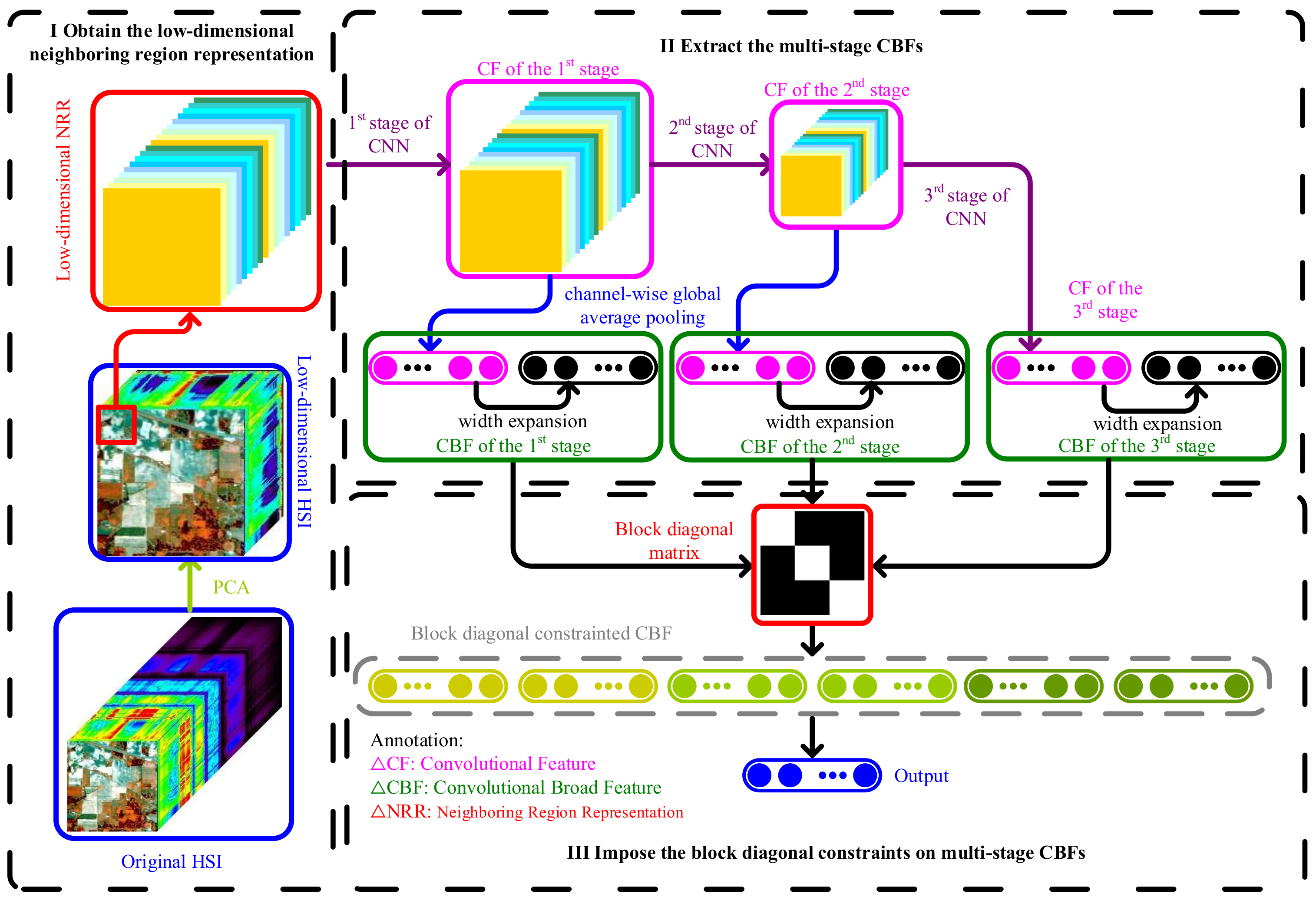
The structure of MSCBL-BD is shown in Figure 1, which mainly includes the following parts: (1) obtaining the low-dimensional neighboring region representation, and using PCA to perform band reduction on the original HSI and constructing the low-dimensional neighboring region representation; (2) extracting the multi-stage CBFs. Firstly, use the limited labeled samples to pre-train a three-stage CNN and extract the multi-stage convolutional features (CFs) of the HSI. Secondly, perform channel-wise global average pooling on the features of the first two stages. Thirdly, perform stage-wise width expansion on the CFs to obtain the broad features (BFs), then further combine the CFs and BFs to obtain the convolutional broad features (CBFs). (3) Imposing the block-diagonal constraints on the multi-stage CBFs. Map the CBFs of all three stages through a block-diagonal matrix to obtain the block-diagonal-constrained CBFs, which ensures that each CBF is only linearly represented by features of the same stage. The optimal solutions of the output layer weight and block-diagonal matrix can be found by the alternating direction method of multipliers (ADMM).
2.2. CNN Pre-Training
The original hyperspectral image is presented in the shape of a 3D cube. If vectorization is performed directly on the HSI, it not only leads to an increase in dimensions, but also destroys the inherent structure of HSI data. The neighboring region representation is a common spectral-spatial representation method in HSIs [48], which is constructed by selecting several pixels around the target pixel. Figure 2 shows a schematic diagram of selecting the surrounding 24 pixels to form a -size neighboring region representation, where B denotes the number of bands in the original HSI. According to this representation, not only the band information of the target pixel but also the information of neighboring pixels can be obtained. Furthermore, if the original high-dimensional neighboring region representation is directly used as the input of the CNN, redundant information will exists in the band and the number of network parameters will increase dramatically, thereby affecting the final performance of the CNN. A common method is utilizing a dimensionality reduction technique, such as principal component analysis (PCA), to reduce the number of bands in the neighboring region representation of an HSI. Define a low-dimensional neighboring region representation as the input data of the CNN, where , , and are the width, height, and number of bands, respectively.
Due to the large amount of parameters of the fully connected layer, the CNN used in our work only includes the convolutional, pooling, nonlinea, and SoftMax layers. The input is connected to the convolutional layer by the convolutional kernel to obtain the output feature maps. The calculation formula is:
where is the bias, represents the output features of the convolution layer, and is the input of the convolutional layer. For the first layer, the input data is the neighboring region representation of the HSI, which is denoted as . indicates the convolutional kernel of the convolutional layer and * represents the convolutional operation. In general, a pooling layer is added after a convolutional layer, which aims to quickly reduce the dimensions and enhance the invariance of the extracted features. The features obtained by the pooling layer are:
where indicates a max-pooling operation and is the input data of the pooling layer, which is also the output of the previous convolutional layer. To achieve nonlinear mapping, a convolutional layer or a pooling layer is typically connected to a nonlinear layer. Here, the activation function of the nonlinear layer is the sigmoid function:
where is the input data of the nonlinear layer, which is also the output of the previous pooling layer; denotes the output nonlinear features of the nonlinear layer. The SoftMax function is generally used as the last layer of the CNN. The number of neurons in the SoftMax layer is equal to the number of classes. The SoftMax loss function is defined as [49]:
where N denotes the number of training samples; C is the number of classes; is the label of the ith sample; and are the weight and bias of the SoftMax layer, respectively; is the input data of the SoftMax layer, which is obtained by the previous multiple convolutional, pooling, and nonlinear calculation procedures; and is the indicator function, so that . The CNN training process consists of two parts: forward and backward calculations. In the forward calculation process, the output of each layer is calculated according to the current parameters. In the backward calculation process, the weight and bias of each layer are updated by minimizing the loss function. The batch stochastic gradient descent algorithm is used for weight and bias update.
Here, one convolutional layer plus one pooling layer plus two nonlinear layers plus one convolutional layer is defined as one stage, and the pre-trained CNN can obtain the multi-stage convolutional feature:
where represents the ith stage feature, ; and s is the total number of stages, denotes the learnable parameter set from the input to the ith stage of the CNN, including convolutional kernels and biases; and denotes the nonlinear mapping procedure of th CNN under .
2.3. MSCBL-BD
The conventional BLS can be regarded as a three-layer neural network, including an input layer, an intermediate layer (composed of an MF and an EN), and an output layer. The MF is obtained by mapping the input with the weights fine-tuned by the linear autoencoder. It is worth noting that the linear features obtained by linear mapping cannot fully express the complex spectral-spatial features of an HSI, thus affecting the final classification performance. The EN is obtained by mapping the MF with random weights to achieve the width expansion of the MF. The output layer is connected to both the MF and the EN. By minimizing the error between the output vector and the ground truth label vector, the objective function of BLS is constructed by:
where the first term is the empirical risk, which aims to calculate the error between the model output vector and the real label vector; denote the labels of the samples; is the -norm; the second term is the structural risk, which is used to improve the generalization ability of the model; and , respectively, represent the features of the MF and EN; indicates the connection weights of the output layer; and is the coefficient of structural risk term. Equation (6) can be solved by ridge regression theory.
Since the linear sparse feature extracted by BLS cannot fully characterize the complex spectral-spatial features of an HSI, the CFs are used to replace the linear sparse features in the MF to achieve more complex nonlinear mapping. Furthermore, in order to reduce the information lost by the CNN in the multi-layer mapping process, the multi-stage features extracted by the CNN are utilized here and separately expanded in width. Given the multi-stage features , the channel-wise global average pooling is first performed on the CFs of the first two stages:
where represents the channel-wise global average pooling, which can summarize the global information of the feature map in each channel, to some extent. After the pooling operation, several 1D vectors are obtained and, together with the CFs of the last stage, constitute the multi-stage CFs (MSCFs) . Furthermore, we expand the MSCFs with random weights to obtain the multi-stage BFs (MSBFs) :
where is the nonlinear function, such as the tansig. Splice the MSCFs and the MSBFs to obtain the MSCBFs and rewrite them as:
Enhancing the linear independence among features can help to produce a more accurate classification model [25,26], so we introduce the block-diagonal constraint [50]. In the commonly used block-diagonal representation method, each sample is represented only by samples with the same class, which can enhance the mutual independence among different classes of samples [51,52]. Here, we use a block matrix to map the MSCBFs into a subspace in which each feature is only represented by those of the same stage. MSCBL-BD optimizes the following objective function:
where denotes the output layer weights of MSCBL-BD. Further consider the error term and rewrite Equation (10) as:
Since the absolute block diagonal structure is difficult to learn, the work of [50] was consulted. Assuming that the components on the non-block diagonal are as small as possible, the incoherent extra stage is boosted, and the coherent intra-stage representation is further enhanced at the same time [50]. Two terms are constructed to achieve the above objectives: (1) is used to minimize the elements on the non-block diagonal, , , where ⊙ is the Hadamard product, denotes the Frobenius norm, is a D-dimensional vector whose elements are all 1; (2) construct a sparse term to enhance the coherent intra-stage representation, where represents the -norm, which can calculate the number of non-zero elements in a matrix, . Here, sparsity here is used to calculate the number of elements that are equal to 0. By minimizing the sparse term, we can make as many elements on the non-diagonal as possible trend to 0. Since the optimization of -norm is NP-hard, a relaxed term is used here, where denotes the -norm. Then, Equation (11) can be rewritten as:
where are the balancing coefficients, is used to explore the potential correlation patterns [53], and denotes the nuclear norm. Due to the difficulty in solving the -norm and the nuclear norm problem, auxiliary variables and are introduced, and Equation (12) can be rewritten as:
Equation (13) can be solved by ADMM [50], and the augmented Lagrangian expression is:
where , , and are Lagrangian multipliers, , and is the penalty parameter. Each variable is updated alternately to find the desired solution and the detailed calculation process of each variable is provided below.
(1) Update . Fixing the other variables, the update process for is equivalent to solving the following objective function:
Calculate the derivative of Equation (15) with respect to and make it zero, then we can obtain the closed solutions:
(2) Update . When the remaining variables are fixed, the expression of Equation (14) about is:
where . Calculate the derivative of Equation (17) with respect to and make it zero; thus, the optimal solution of is:
where , , and .
(3) Update . Fix the other variables and abbreviate Equation (14) as an expression only for variable :
According to [54], the solution can be obtained by using the singular value threshold operation:
where is the singular value decomposition of , and is the soft threshold operation, which is defined as:
where is a threshold value.
(4) Update . The update process of variable is equivalent to solving the following problem:
which can be updated by the point multiplication mechanism, and the optimal solution is calculated as follows:
where .
(5) Update . When fixing the other variables, we rewrite the objective function of Equation (14) on variable and obtain:
According to [50], let and
The above steps are alternated until a predetermined maximum number of iterations is reached, thereby obtaining the desired output layer weight and the block diagonal matrix , and further calculating the prediction label vector :
Consequently, sparse signal recovery problems can be solved by a dozen different methods, such as orthogonal matching pursuit, K-SVD, ADMM, etc. Among them, ADMM was designed for general decomposition methods and decentralized algorithms in optimization problems. Furthermore, many state-of-the-art algorithms for -norm-involved problems can be derived by ADMM. In addition, the problem in Equation (13) can be seen as a special case of the classical ADMM problem. Therefore, ADMM is used here to solve the problem in Equation (13).
3. Experiments and Analysis
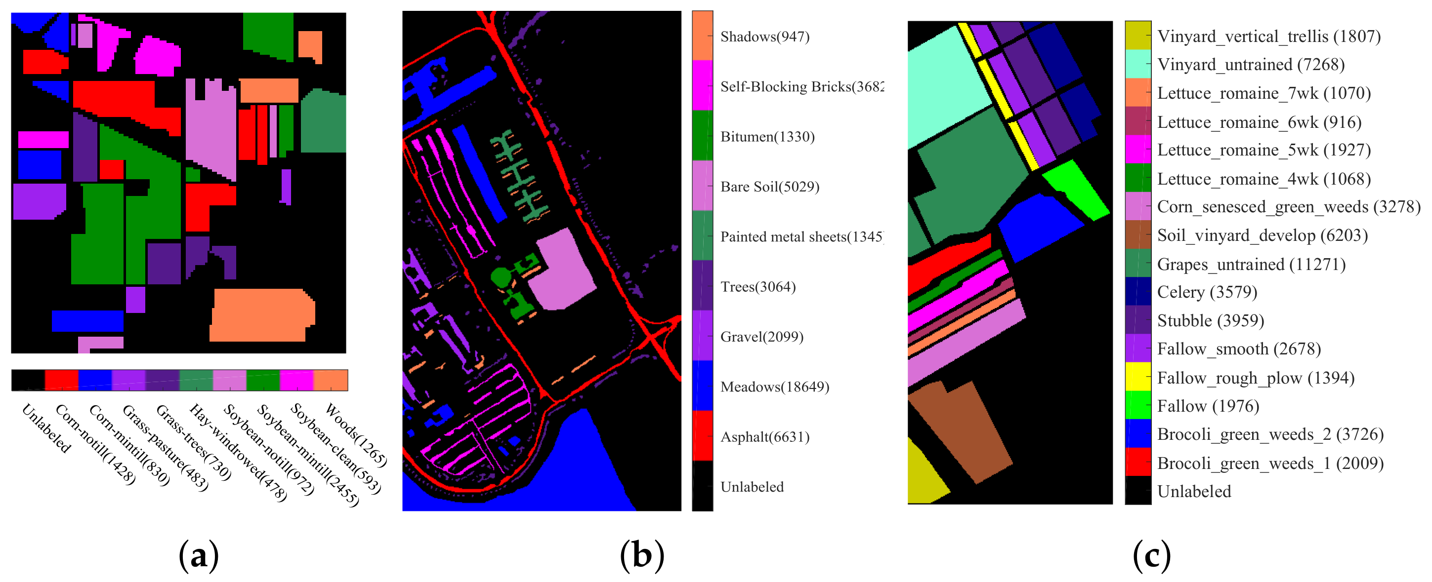
To verify the validity of the proposed method, we selected three popular real HSI datasets: Indian Pines, Pavia University, and Salinas. The ground-truth maps and sample information of the three HSI datasets are shown in Figure 3. The spatial resolutions of the three datasets are , , and , respectively. All experiments were performed on the MATLAB 2016a platform;the used computer was configured as: CPU Intel I7-4790, 16 G memory, and GPU GTX980. In order to eliminate the randomness, all experiments were repeated 10 times to obtain the mean values. A total of 200 labeled samples per class were randomly selected for training and the others were used for testing. Four evaluation indicators were selected to evaluate the experimental results, which were the classification accuracy of each class of ground object, the average classification accuracy (AA), the overall classification accuracy (OA) and the Kappa coefficient.
3.1. Parameter Setting
Except for the number of feature maps of the last convolutional layer (the numbers of feature maps are 9, 9, and 16 for the Indian Pines, Pavia University, and Salinas datasets, respectively), the network structures of the CNNs for three HSI datasets were the same. The detailed structure of the CNN is shown in Table 1. It can be seen that: (1) there were total 5 convolutional layers, i.e., C1∼C5. The convolutional kernel sizes of C2 and C4 were , which is helpful for obtaining a deeper network structure at the cost of a small increase in network parameters. The convolutional kernel sizes of C1 and C3 were , the convolutional kernel size of C5 was . (2) There were two max-pooling layers, i.e., P1 and P2, both step sizes of which were 2. (3) A total of 4 nonlinear layers denoted as N1∼N4 were included. The activation functions used in all of the nonlinear layers were the Sigmoid function.
The CNN training process consists of two steps: forward calculation and back propagation. The former aims to calculate the classification result based on the current network parameters, and the latter updates the network parameters. Here, we used a stochastic gradient descent algorithm to update the CNN with a batch size of 100, a learning rate of 0.1, and an iteration of 1000. The CNN training process is based on the Matconvnet toolbox [55].
The parameter settings of MSCBL-BD on the three datasets are shown in Table 2, where are tuned to achieve the best performance via fivefold cross-validations from .
3.2. Comparative Experiments
In order to verify the validity of the proposed MSCBL-BD, six benchmark methods and two special cases of MSCBL-BD (CBL and MSCBL) were selected for comparative experiments:
- (1)
- Traditional classification methods: SVM [8], whose optimal super-parameters are selected through the fivefold cross-validation method;
- (2)
- (3)
- Special cases of MSCBL-BD: CBL (the CBFs of the last stage are connected to the output layer and not constrained with the block diagonal matrix); MSCBL (the MSCBFs are connected to the output layer and not constrained with the block-diagonal matrix).
4. Discussion
From the experimental results, we can see that: (1) On all of three HSI datasets, for three evaluation indexes (AA, OA, and Kappa coefficients), MSCBL-BD, MSCBL, and CBL achieved higher performance than the other methods. Taking the Indian Pines dataset as an example, CBL outperformed BLS by 11.52% in terms of OA. The main reasons are two-fold: the features learned by BLS are linear sparse features and only the spectral information is utilized. Therefore, the features of the HSI cannot be fully represented. In addition, CBL, MSCBL, and MSCBL-BD outperformed CNN by 1.68%, 2.7%, and 3.91% on the OA, respectively, which verifies the superiority of width expansion. (2) On the three HSI datasets, MSCBL outperformed CBL by 1.02%, 0.24%, and 0.45%, respectively, because MSCBL utilizes the MSCFs and performs feature expansion for each stage, which makes the features learned by MSCBL more discriminative. Furthermore, MSCBL-BD outperformed MSCBL by 1.21%, 0.15%, and 0.6% on the three datasets, respectively, because the MSCBFs are mapped through a block-diagonal matrix, so that each obtained feature is linearly represented only by the features of its own stage, thereby enhancing the linear independence of the MSCBFs of each stage. This can help with learning a more accurate HSI classification model, which in turn improves the final classification accuracy. (3) Both SS-DBN and CNN are deep spectral-spatial classification methods. Compared with SS-DBN, CNN yielded higher OAs on all HSI datasets. This is because SS-DBN takes features by stacking the spectral vector and the vectorized neighboring region representation as the input of the DBN, which not only leads to an increase in the dimension of the input data, but also destroys the inherent structure of the data. In addition, in the case of a small number of labeled samples, as a kind of fully-connected neural network, over-fitting may occur in the training process of SS-DBN. Figure 4, Figure 5 and Figure 6 show the classification maps achieved by different methods. It can be seen that the classification maps obtained by MSCBL-BD on all of three HSI datasets are smoother and more detailed. Taking the Indian Pines dataset as an example, the benchmark methods misclassify more Soybean-clean, Soybean-notill, and Corn-notill as Soybean-mintill; misclassify more Grass-trees into Woods; and misclassify more Corn-notill into Corn-minitill.
5. Conclusions
A novel BLS based method (MSCBL-BD) for HSI classification was proposed in this paper. By replacing the linear sparse features with convolutional features, the nonlinear mapping ability of the model is improved and the complex spectral-spatial features of HSI can be better represented. Therefore, the CBL has higher classification accuracy than BLS. Furthermore, in order to reduce the information loss occurring in the multi-layer mapping process of CNN, the MSCBFs are utilized. Moreover, in order to train a more accurate HSI classification model, the block-diagonal constraint is introduced to the MSCBL. The MSCBFs are mapped by a block-diagonal matrix, and the obtained features are only linearly represented by those of their own stages. Therefore, the linear independence of the MSCBFs is enhanced and the classification accuracy is improved ultimately. The experimental results demonstrated the superiority of MSCBL-BD compared to some competitive methods. In our future work, we will increase the robustness of our method, so that satisfactory performance can be achieved when bands are missing.
Author Contributions
All of the authors provided significant contributions to the work. Y.K. and X.W. conceived and designed the experiments; Y.K. and X.W. performed the experiments; Y.K. and Y.C. analyzed the data; Y.K. and Y.C. wrote the original paper; C.L.P.C. reviewed and edited the paper. All authors have read and agreed to the published version of the manuscript.
Funding
This research was funded by the National Natural Science Foundation of China under grants 62006232, 61976215, 61772532. This research was also funded by the Natural Science Foundation of Jiangsu Province under grant BK20200632.
Data Availability Statement
Publicly available datasets were analyzed in this study. These data can be found: http://www.ehu.eus/ccwintco/index.php?title=Hyperspectral_Remote_Sensing_Scenes accessed on 15 July 2018.
Conflicts of Interest
The authors declare no conflict of interest.
Abbreviations
The following abbreviations are used in this manuscript:
| ADMM | Alternating direction method of multipliers |
| BASS-Net | Band-adaptive spectral-spatial feature learning neural network |
| BF | Broad feature |
| BLS | Broad learning system |
| CBF | Convolutional broad feature |
| CF | Convolutional feature |
| CNN | Convolutional neural network |
| CNN-PPF | Convolutional neural network with pixel-pair features |
| DBN | Deep belief network |
| EN | Enhancement node |
| HSI | Hyperspectral image |
| MF | Mapped feature |
| MSBF | Multi-stage broad feature |
| MSCBF | Multi-stage convolutional broad feature |
| MSCBL-BD | Block-diagonal constrained multi-stage convolutional broad learning |
| MSCF | Multi-stage convolutional feature |
| PCA | Principal component analysis |
| SS-DBN | Spectral-spatial deep belief network |
| SVM | Support vector machine |
References
- Luo, F.; Du, B.; Zhang, L.; Zhang, L.; Tao, D. Feature learning using spatial-spectral hypergraph discriminant analysis for hyperspectral image. IEEE Trans. Cybern. 2019, 49, 2406–2419. [Google Scholar] [CrossRef] [PubMed]
- Zhou, Y.; Wei, Y. Learning hierarchical spectral-spatial features for hyperspectral image classification. IEEE Trans. Cybern. 2016, 46, 1667–1678. [Google Scholar] [CrossRef] [PubMed]
- Meroni, M.; Fasbender, D.; Balaghi, R.; Dali, M.; Haffani, M.; Haythem, I.; Hooker, J.; Lahlou, M.; Lopez-Lozano, R.; Mahyou, H.; et al. Evaluating NDVI data continuity between SPOT-VEGETATION and PROBA-V missions for operational yield forecasting in North African countries. IEEE Trans. Geosci. Remote Sens. 2016, 54, 795–804. [Google Scholar] [CrossRef]
- Brunet, D.; Sills, D. A generalized distance transform: Theory and applications to weather analysis and forecasting. IEEE Trans. Geosci. Remote Sens. 2017, 55, 1752–1764. [Google Scholar] [CrossRef]
- Islam, T.; Hulley, G.C.; Malakar, N.K.; Radocinski, R.G.; Guillevic, P.C.; Hook, S.J. A Physics-based algorithm for the simultaneous retrieval of land surface temperature and emissivity from VIIRS thermal infrared data. IEEE Trans. Geosci. Remote Sens. 2017, 55, 563–576. [Google Scholar] [CrossRef]
- Matsuki, T.; Yokoya, N.; Iwasaki, A. Hyperspectral tree species classification of Japanese complex mixed forest with the aid of lidar data. IEEE J. Sel. Topics Appl. Earth Observ. Remote Sens. 2015, 8, 2177–2187. [Google Scholar] [CrossRef]
- Liu, L.; Huang, W.; Wang, C. Hyperspectral image classification with kernel-based least-squares support vector machines in sum space. IEEE J. Sel. Top. Appl. Earth Observ. Remote Sens. 2018, 11, 1144–1157. [Google Scholar] [CrossRef]
- Tan, K.; Zhang, J.; Du, Q.; Wang, X. GPU parallel implementation of support vector machines for hyperspectral image classification. IEEE J. Sel. Top. Appl. Earth Observ. Remote Sens. 2015, 8, 4647–4656. [Google Scholar] [CrossRef]
- Ma, L.; Crawford, M.; Tian, J. Local manifold learning-based k-nearest-neighbor for hyperspectral image classification. IEEE Trans. Geosci. Remote Sens. 2010, 48, 4099–4109. [Google Scholar] [CrossRef]
- Bioucas-Dias, J.; Plaza, A.; Camps-Valls, G.; Scheunders, P.; Nasrabadi, N.; Chanussot, J. Hyperspectral remote sensing data analysis and future challenges. IEEE Geosci. Remote Sens. Mag. 2013, 1, 6–36. [Google Scholar] [CrossRef] [Green Version]
- Sun, W.; Halevy, A.; Benedetto, J.; Czaja, W.; Liu, C.; Wu, H.; Shi, B.; Li, W. UL-Isomap based nonlinear dimensionality reduction for hyperspectral imagery classification. ISPRS J. Photogramm. Remote Sens. 2014, 89, 25–36. [Google Scholar] [CrossRef]
- Sun, W.; Yang, G.; Du, B.; Zhang, L.; Zhang, L. A sparse and low-rank near-isometric linear embedding method for feature extraction in hyperspectral imagery classification. IEEE Trans. Geosci. Remote Sens. 2017, 55, 4032–4046. [Google Scholar] [CrossRef]
- Zhang, L.; Zhang, Q.; Du, B.; Huang, X.; Tang, Y.Y.; Tao, D. Simultaneous spectral-spatial feature selection and extraction for hyperspectral images. IEEE Trans. Cybern. 2018, 48, 16–28. [Google Scholar] [CrossRef] [PubMed] [Green Version]
- Li, W.; Liu, J.; Du, Q. Sparse and low-rank graph for discriminant analysis of hyperspectral imagery. IEEE Trans. Geosci. Remote Sens. 2016, 54, 4094–4105. [Google Scholar] [CrossRef]
- Huang, H.; Shi, G.; He, H.; Duan, Y.; Luo, F. Dimensionality reduction of hyperspectral imagery based on spatial-spectral manifold learning. IEEE Trans. Cybern. 2020, 50, 2604–2616. [Google Scholar] [CrossRef] [Green Version]
- Pan, L.; Li, H.; Li, W.; Chen, X.; Wu, G.; Du, Q. Discriminant analysis of hyperspectral imagery using fast kernel sparse and low-rank graph. IEEE Trans. Geosci. Remote Sens. 2017, 55, 6085–6098. [Google Scholar] [CrossRef]
- Pan, L.; Li, H.; Deng, Y.; Zhang, F.; Chen, X.; Du, Q. Hyperspectral dimensionality reduction by tensor sparse and low-rank graph-based discriminant analysis. Remote Sens. 2017, 9, 452. [Google Scholar] [CrossRef] [Green Version]
- Dong, Y.; Du, B.; Zhang, L.; Zhang, L. Dimensionality reduction and classification of hyperspectral images using ensemble discriminative local metric learning. IEEE Trans. Geosci. Remote Sens. 2017, 55, 2509–2524. [Google Scholar] [CrossRef]
- Dong, Y.; Du, B.; Zhang, L.; Zhang, L. Exploring locally adaptive dimensionality reduction for hyperspectral image classification: A maximum margin metric learning aspect. IEEE J. Sel. Top. Appl. Earth Observ. Remote Sens. 2017, 10, 1136–1150. [Google Scholar] [CrossRef]
- Kang, X.; Xiang, X.; Li, S.; Benediktsson, J. PCA-based edge-preserving features for hyperspectral image classification. IEEE Trans. Geosci. Remote Sens. 2017, 55, 7140–7151. [Google Scholar] [CrossRef]
- Jia, S.; Shen, L.; Zhu, J.; Li, Q. A 3-D Gabor phase-based coding and matching framework for hyperspectral imagery classification. IEEE Trans. Cybern. 2018, 48, 1176–1188. [Google Scholar] [CrossRef]
- Zhang, L.; Zhang, L.; Tao, D.; Huang, X. On combining multiple features for hyperspectral remote sensing image classification. IEEE Trans. Geosci. Remote Sens. 2012, 50, 879–893. [Google Scholar] [CrossRef]
- Li, J.; Huang, X.; Gamba, P.; Bioucas-Dias, J.; Zhang, L.; Benediktsson, J.; Plaza, A. Multiple feature learning for hyperspectral image classification. IEEE Trans. Geosci. Remote Sens. 2015, 53, 1592–1606. [Google Scholar] [CrossRef] [Green Version]
- Liu, Z.; Chen, C.L.P. Broad learning system: Structural extensions on single-layer and multi-layer neural networks. In Proceedings of the International Conference on Security, Pattern Analysis, and Cybernetics, Shenzhen, China, 15–18 December 2017; pp. 136–141. [Google Scholar]
- Chen, C.L.P.; Liu, Z. Broad learning system: An effective and efficient incremental learning system without the need for deep architecture. IEEE Trans. Neural Netw. Learn. Syst. 2018, 29, 10–24. [Google Scholar] [CrossRef] [PubMed]
- Chen, C.L.P.; Liu, Z.; Feng, S. Universal approximation capability of broad learning system and its structural variations. IEEE Trans. Neural Netw. Learn. Syst. 2019, 30, 1191–1204. [Google Scholar] [CrossRef] [PubMed]
- Feng, S.; Chen, C.L.P. Fuzzy broad learning system: A novel neuro-fuzzy model for regression and classification. IEEE Trans. Cybern. 2020, 50, 414–424. [Google Scholar] [CrossRef] [PubMed]
- Kong, Y.; Wang, X.; Cheng, Y.; Chen, C.L.P. Hyperspectral imagery classification based on semi-supervised broad learning system. Remote Sens. 2018, 10, 685. [Google Scholar] [CrossRef] [Green Version]
- Lecun, Y.; Bengio, Y.; Hinton, G. Deep learning. Nature 2015, 521, 436–444. [Google Scholar] [CrossRef] [PubMed]
- Zhang, L.; Zhang, L.; Du, B. Deep learning for remote sensing data: A technical tutorial on the state of the art. IEEE Geosci. Remote Sens. Mag. 2016, 4, 22–40. [Google Scholar] [CrossRef]
- Zhu, X.; Tuia, D.; Mou, L.; Xia, G.; Zhang, L.; Xu, F.; Fraundorfer, F. Deep learning in remote sensing: A comprehensive review and list of resources. IEEE Geosci. Remote Sens. Mag. 2017, 5, 8–36. [Google Scholar] [CrossRef] [Green Version]
- Zhang, T.; Su, G.; Qing, C.; Xu, X.; Cai, B.; Xing, X. Hierarchical lifelong learning by sharing representations and integrating hypothesis. IEEE Trans. Syst. Man Cybern. Syst. 2021, 51, 1004–1014. [Google Scholar] [CrossRef]
- Chen, Y.; Lin, Z.; Zhao, X.; Wang, G.; Gu, Y. Deep learning-based classification of hyperspectral data. IEEE J. Sel. Top. Appl. Earth Observ. Remote Sens. 2014, 7, 2094–2107. [Google Scholar] [CrossRef]
- Chen, Y.; Zhao, X.; Jia, X. Spectral-spatial classification of hyperspectral data based on deep belief network. IEEE J. Sel. Top. Appl. Earth Observ. Remote Sens. 2015, 8, 2381–2392. [Google Scholar] [CrossRef]
- Ma, X.; Wang, H.; Geng, J. Spectral-spatial classification of hyperspectral image based on deep auto-encoder. IEEE J. Sel. Top. Appl. Earth Observ. Remote Sens. 2016, 9, 4073–4085. [Google Scholar] [CrossRef]
- Zhong, P.; Gong, Z.; Li, S.; Schönlieb, C.B. Learning to diversify deep belief networks for hyperspectral image classification. IEEE Trans. Geosci. Remote Sens. 2017, 55, 3516–3530. [Google Scholar] [CrossRef]
- Zhou, X.; Li, S.; Tang, F.; Qin, K.; Hu, S.; Liu, S. Deep learning with grouped features for spatial spectral classification of hyperspectral images. IEEE Geosci. Remote Sens. Lett. 2017, 14, 97–101. [Google Scholar] [CrossRef]
- Romero, A.; Gatta, C.; Camps-Valls, G. Unsupervised deep feature extraction for remote sensing image classification. IEEE Trans. Geosci. Remote Sens. 2016, 54, 1349–1362. [Google Scholar] [CrossRef] [Green Version]
- Makantasis, K.; Karantzalos, K.; Doulamis, A.; Doulamis, N. Deep supervised learning for hyperspectral data classification through convolutional neural networks. In Proceedings of the 2015 IEEE International Geoscience and Remote Sensing Symposium, Milan, Italy, 26–31 July 2015; pp. 4959–4962. [Google Scholar]
- Chen, Y.; Jiang, H.; Li, C.; Jia, X.; Ghamisi, P. Deep feature extraction and classification of hyperspectral images based on convolutional neural networks. IEEE Trans. Geosci. Remote Sens. 2016, 54, 6232–6251. [Google Scholar] [CrossRef] [Green Version]
- Zhao, W.; Du, S. Spectral-spatial feature extraction for hyperspectral image classification: A dimension reduction and deep learning approach. IEEE Trans. Geosci. Remote Sens. 2016, 54, 4544–4554. [Google Scholar] [CrossRef]
- Ghamisi, P.; Chen, Y.; Zhu, X. A self-improving convolution neural network for the classification of hyperspectral data. IEEE Geosci. Remote Sens. Lett. 2016, 13, 1537–1541. [Google Scholar] [CrossRef] [Green Version]
- Santara, A.; Mani, K.; Hatwar, P.; Singh, A.; Garg, A.; Padia, K.; Mitra, P. BASS net: Band-adaptive spectral-spatial feature learning neural network for hyperspectral image classification. IEEE Trans. Geosci. Remote Sens. 2017, 55, 5293–5301. [Google Scholar] [CrossRef] [Green Version]
- Chan, T.; Jia, K.; Gao, S.; Lu, J.; Zeng, Z.; Ma, Y. PCANet: A simple deep learning baseline for image classification. IEEE Trans. Image Process. 2015, 24, 5017–5032. [Google Scholar] [CrossRef] [PubMed] [Green Version]
- Pan, B.; Shi, Z.; Zhang, N.; Xie, S. Hyperspectral image classification based on nonlinear spectral-spatial network. IEEE Geosci. Remote Sens. Lett. 2016, 13, 1782–1786. [Google Scholar] [CrossRef]
- Pan, B.; Shi, Z.; Xu, X. R-VCANet: A new deep-learning-based hyperspectral image classification method. IEEE J. Sel. Topics Appl. Earth Observ. Remote Sens. 2017, 10, 1975–1986. [Google Scholar] [CrossRef]
- Li, W.; Wu, G.; Zhang, F.; Du, Q. Hyperspectral image classification using deep pixel-pair features. IEEE Trans. Geosci. Remote Sens. 2017, 55, 844–853. [Google Scholar] [CrossRef]
- Gao, Y.; Wang, X.; Cheng, Y.; Wang, Z. Dimensionality reduction for hyperspectral data based on class-aware tensor neighborhood graph and patch alignment. IEEE Trans. Neural Netw. Learn. Sys. 2015, 26, 1582–1593. [Google Scholar]
- Jin, J.; Fu, K.; Zhang, C. Traffic sign recognition with hinge loss trained convolutional neural networks. IEEE Trans. Intell. Transp. Syst. 2014, 15, 1991–2000. [Google Scholar] [CrossRef]
- Zhang, Z.; Xu, Y.; Shao, L.; Yang, J. Discriminative block-diagonal representation learning for image recognition. IEEE Trans. Neural Netw. Learn. Syst. 2017, 29, 3111–3125. [Google Scholar] [CrossRef] [PubMed] [Green Version]
- Wang, Q.; He, X.; Li, X. Locality and structure regularized low rank representation for hyperspectral image classification. IEEE Trans. Geosci. Remote Sens. 2019, 57, 911–923. [Google Scholar] [CrossRef] [Green Version]
- Wang, J.; Wang, X.; Tian, F.; Liu, C.H.; Yu, H. Constrained low-rank representation for robust subspace clustering. IEEE Trans. Cybern. 2017, 47, 4534–4546. [Google Scholar] [CrossRef] [Green Version]
- Liu, G.; Lin, Z.; Yan, S.; Sun, J.; Yu, Y.; Ma, Y. Robust recovery of subspace structures by low-rank representation. IEEE Trans. Pattern Anal. Mach. Intell. 2013, 35, 171–184. [Google Scholar] [CrossRef] [PubMed] [Green Version]
- Cai, J.-F.; Candès, E.J.; Shen, Z. A singular value thresholding algorithm for matrix completion. SIAM J. Optim. 2010, 20, 1956–1982. [Google Scholar] [CrossRef]
- Vedaldi, A.; Lenc, K. Matconvnet-convolutional neural networks for matlab. In Proceedings of the ACM International Conference on Multimedia, Orlando, FL, USA, 3–7 November 2014; pp. 689–692. [Google Scholar]
Figure 1.
Structure diagram of MSCBL-BD.

Figure 2.
-size neighboring region representation of an HSI.

Figure 3.
Ground-truth maps and sample information of different hyperspectral datasets: (a) Indian Pines ( spatial resolution); (b) Pavia University ( spatial resolution); (c) Salinas ( spatial resolution). The number of samples contained in each class is shown after the class name.
Figure 3.
Ground-truth maps and sample information of different hyperspectral datasets: (a) Indian Pines ( spatial resolution); (b) Pavia University ( spatial resolution); (c) Salinas ( spatial resolution). The number of samples contained in each class is shown after the class name.

Figure 4.
Classification maps obtained by different methods on the Indian Pines dataset: (a) SVM; (b) BLS; (c) SS-DBN; (d) CNN-PPF; (e) CNN; (f) CBL; (g) MSCBL; (h) MSCBL-BD.
Figure 4.
Classification maps obtained by different methods on the Indian Pines dataset: (a) SVM; (b) BLS; (c) SS-DBN; (d) CNN-PPF; (e) CNN; (f) CBL; (g) MSCBL; (h) MSCBL-BD.

Figure 5.
Classification maps obtained by different methods on the Pavia University dataset: (a) SVM; (b) BLS; (c) SS-DBN; (d) CNN-PPF; (e) CNN; (f) CBL; (g) MSCBL; (h) MSCBL-BD.
Figure 5.
Classification maps obtained by different methods on the Pavia University dataset: (a) SVM; (b) BLS; (c) SS-DBN; (d) CNN-PPF; (e) CNN; (f) CBL; (g) MSCBL; (h) MSCBL-BD.

Figure 6.
Classification maps obtained by the different methods on the Salinas dataset: (a) SVM; (b) BLS; (c) SS-DBN; (d) CNN-PPF; (e) CNN; (f) CBL; (g) MSCBL; (h) MSCBL-BD.
Figure 6.
Classification maps obtained by the different methods on the Salinas dataset: (a) SVM; (b) BLS; (c) SS-DBN; (d) CNN-PPF; (e) CNN; (f) CBL; (g) MSCBL; (h) MSCBL-BD.


Table 1.
Configuration of the CNN.
| Layer | Input | Number of Filters | Width of Filters | Height of Filters | Step Size | Output | |||||
|---|---|---|---|---|---|---|---|---|---|---|---|
| Width | Height | Channel | Width | Height | Channel | Dimension | |||||
| I1 | 17 | 17 | 15 | 4335 | |||||||
| C1 | 17 | 17 | 15 | 30 | 4 | 4 | 1 | 14 | 14 | 30 | 5880 |
| P1 | 14 | 14 | 30 | 2 | 2 | 2 | 7 | 7 | 30 | 1470 | |
| N1 | 7 | 7 | 30 | / | / | / | / | 7 | 7 | 30 | 1470 |
| C2 | 7 | 7 | 30 | 30 | 1 | 1 | 1 | 7 | 7 | 30 | 1470 |
| N2 | 7 | 7 | 30 | 30 | 1 | 1 | 1 | 7 | 7 | 30 | 1470 |
| C3 | 7 | 7 | 30 | 30 | 4 | 4 | 1 | 4 | 4 | 30 | 480 |
| P3 | 4 | 4 | 30 | / | 2 | 2 | 2 | 2 | 2 | 30 | 120 |
| N3 | 2 | 2 | 30 | / | / | / | / | 2 | 2 | 30 | 120 |
| C4 | 2 | 2 | 30 | 30 | 1 | 1 | 1 | 2 | 2 | 30 | 120 |
| N4 | 2 | 2 | 30 | / | / | / | / | 2 | 2 | 30 | 120 |
| C5 | 2 | 2 | 30 | 9/16 | 2 | 2 | 1 | 1 | 1 | 9/16 | 9/16 |
| Softmax | 1 | 1 | 9/16 | / | / | / | / | 1 | 1 | 9/16 | 9/16 |
Table 2.
Parameter settings of MSCBL-BD.
| Number of Iterations | Number of Nodes in EN | ||
|---|---|---|---|
| Indian Pines | 500 | ||
| Pavia University | 110 | 400 | |
| Salinas | 500 |
Table 3.
Comparison of the classification performance on the Indian Pines dataset.
| SVM [8] | BLS [25] | SS-DBN [34] | CNN-PPF [47] | CNN [39] | CBL | MSCBL | MSCBL-BD | |
|---|---|---|---|---|---|---|---|---|
| A1 (%) | 75.49 | 82.54 | 77.20 | 92.23 | 89.98 | 92.84 | 94.14 | 96.58 |
| A2 (%) | 73.78 | 82.29 | 82.76 | 96.69 | 97.75 | 98.43 | 99.06 | 99.32 |
| A3 (%) | 95.26 | 95.26 | 94.42 | 99.86 | 98.80 | 99.40 | 99.82 | 100 |
| A4 (%) | 98.45 | 99.10 | 98.30 | 99.43 | 99.21 | 99.68 | 99.85 | 99.96 |
| A5 (%) | 99.71 | 99.71 | 99.86 | 99.86 | 99.93 | 100 | 100 | 100 |
| A6 (%) | 78.21 | 86.68 | 87.23 | 95.10 | 94.69 | 96.22 | 97.20 | 99.02 |
| A7 (%) | 66.18 | 69.65 | 76.02 | 89.48 | 89.59 | 92.28 | 94.12 | 95.96 |
| A8 (%) | 83.77 | 93.39 | 90.59 | 97.00 | 98.19 | 98.93 | 99.42 | 99.87 |
| A9 (%) | 98.27 | 98.91 | 94.93 | 99.89 | 99.02 | 99.54 | 99.81 | 99.81 |
| AA (%) | 85.46 | 89.73 | 89.04 | 96.62 | 96.35 | 97.48 | 98.16 | 98.95 |
| OA (%) | 79.80 | 84.26 | 84.61 | 94.51 | 94.10 | 95.78 | 96.80 | 98.01 |
| Kappa | 0.7611 | 0.8142 | 0.8178 | 0.9344 | 0.9296 | 0.9495 | 0.9617 | 0.9762 |
Table 4.
Comparison of the classification performance on the Pavia University dataset.
| SVM [8] | BLS [25] | SS-DBN [34] | CNN-PPF [47] | CNN [39] | CBL | MSCBL | MSCBL-BD | |
|---|---|---|---|---|---|---|---|---|
| A1 (%) | 83.35 | 76.32 | 81.46 | 97.40 | 96.68 | 97.21 | 97.78 | 98.25 |
| A2 (%) | 86.12 | 90.13 | 92.96 | 97.40 | 98.93 | 99.10 | 99.27 | 99.39 |
| A3 (%) | 83.23 | 82.59 | 88.37 | 92.29 | 97.91 | 98.40 | 98.78 | 98.79 |
| A4 (%) | 94.66 | 95.49 | 95.55 | 97.63 | 98.54 | 98.62 | 98.80 | 98.80 |
| A5 (%) | 99.55 | 99.62 | 99.91 | 99.93 | 99.89 | 99.97 | 100 | 99.99 |
| A6 (%) | 88.87 | 91.25 | 88.92 | 97.89 | 99.64 | 99.96 | 99.96 | 99.92 |
| A7 (%) | 90.48 | 94.67 | 90.35 | 97.33 | 99.11 | 99.58 | 99.74 | 99.83 |
| A8 (%) | 84.39 | 84.54 | 85.93 | 93.97 | 98.31 | 98.27 | 98.73 | 98.96 |
| A9 (%) | 99.90 | 99.65 | 99.49 | 99.57 | 99.69 | 99.80 | 99.84 | 99.85 |
| AA (%) | 90.06 | 90.47 | 91.44 | 97.05 | 98.74 | 98.99 | 99.21 | 99.31 |
| OA (%) | 87.07 | 88.21 | 90.29 | 97.05 | 98.58 | 98.82 | 99.06 | 99.21 |
| Kappa | 0.8301 | 0.8445 | 0.8708 | 0.9626 | 0.9809 | 0.9842 | 0.9873 | 0.9893 |
Table 5.
Comparison of the classification performance on the Salinas dataset.
| SVM [8] | BLS [25] | SS-DBN [34] | CNN-PPF [47] | CNN [39] | CBL | MSCBL | MSCBL-BD | |
|---|---|---|---|---|---|---|---|---|
| A1 (%) | 99.14 | 99.60 | 98.94 | 99.86 | 99.97 | 99.98 | 100 | 100 |
| A2 (%) | 99.45 | 99.65 | 98.95 | 99.59 | 99.95 | 99.98 | 100 | 100 |
| A3 (%) | 99.46 | 99.46 | 79.60 | 99.83 | 99.46 | 99.85 | 99.93 | 99.90 |
| A4 (%) | 99.58 | 99.43 | 99.58 | 99.68 | 99.51 | 99.92 | 99.91 | 99.93 |
| A5 (%) | 98.79 | 99.28 | 99.71 | 98.41 | 98.94 | 99.40 | 99.53 | 99.76 |
| A6 (%) | 99.79 | 99.81 | 99.91 | 99.78 | 100 | 100 | 100 | 100 |
| A7 (%) | 99.67 | 99.57 | 98.90 | 99.85 | 99.87 | 99.95 | 99.98 | 99.99 |
| A8 (%) | 84.40 | 83.18 | 87.04 | 83.28 | 85.61 | 91.05 | 92.41 | 94.24 |
| A9 (%) | 99.37 | 99.75 | 97.93 | 97.44 | 99.31 | 99.47 | 99.55 | 99.63 |
| A10 (%) | 94.65 | 95.76 | 95.79 | 95.84 | 98.98 | 99.44 | 99.64 | 99.72 |
| A11 (%) | 98.87 | 98.66 | 98.64 | 99.75 | 99.60 | 99.88 | 99.94 | 99.90 |
| A12 (%) | 99.95 | 100 | 99.73 | 100 | 99.90 | 99.95 | 99.94 | 99.98 |
| A13 (%) | 99.52 | 99.16 | 99.50 | 99.38 | 100 | 100 | 100 | 100 |
| A14 (%) | 97.91 | 98.12 | 99.95 | 99.52 | 99.79 | 99.96 | 100 | 100 |
| A15 (%) | 69.35 | 73.82 | 85.92 | 81.18 | 95.12 | 95.02 | 95.90 | 97.17 |
| A16 (%) | 99.02 | 98.94 | 99.75 | 98.51 | 99.84 | 99.89 | 99.91 | 99.97 |
| AA (%) | 96.19 | 96.51 | 96.24 | 96.99 | 98.49 | 98.98 | 99.16 | 99.39 |
| OA (%) | 91.67 | 92.18 | 93.76 | 92.98 | 95.94 | 97.22 | 97.67 | 98.27 |
| Kappa | 0.9067 | 0.9125 | 0.9302 | 0.9215 | 0.9546 | 0.9689 | 0.9740 | 0.9807 |
Publisher’s Note: MDPI stays neutral with regard to jurisdictional claims in published maps and institutional affiliations. |
© 2021 by the authors. Licensee MDPI, Basel, Switzerland. This article is an open access article distributed under the terms and conditions of the Creative Commons Attribution (CC BY) license (https://creativecommons.org/licenses/by/4.0/).
Share and Cite
MDPI and ACS Style
Kong, Y.; Wang, X.; Cheng, Y.; Chen, C.L.P. Multi-Stage Convolutional Broad Learning with Block Diagonal Constraint for Hyperspectral Image Classification. Remote Sens. 2021, 13, 3412. https://0-doi-org.brum.beds.ac.uk/10.3390/rs13173412
AMA Style
Kong Y, Wang X, Cheng Y, Chen CLP. Multi-Stage Convolutional Broad Learning with Block Diagonal Constraint for Hyperspectral Image Classification. Remote Sensing. 2021; 13(17):3412. https://0-doi-org.brum.beds.ac.uk/10.3390/rs13173412
Chicago/Turabian StyleKong, Yi, Xuesong Wang, Yuhu Cheng, and C. L. Philip Chen. 2021. "Multi-Stage Convolutional Broad Learning with Block Diagonal Constraint for Hyperspectral Image Classification" Remote Sensing 13, no. 17: 3412. https://0-doi-org.brum.beds.ac.uk/10.3390/rs13173412
Note that from the first issue of 2016, this journal uses article numbers instead of page numbers. See further details here.