Article

Forest Conservation with Deep Learning: A Deeper Understanding of Human Geography around the Betampona Nature Reserve, Madagascar

1
Geospatial Institute, Saint Louis University, St. Louis, MO 63108, USA
2
Department of Earth and Atmospheric Sciences, Saint Louis University, St. Louis, MO 63108, USA
3
Madagascar Fauna and Flora Group, Kalinka, Lochearnhead FK19 8NZ, UK
*
Author to whom correspondence should be addressed.
Remote Sens. 2021, 13(17), 3495; https://0-doi-org.brum.beds.ac.uk/10.3390/rs13173495
Submission received: 17 July 2021 / Revised: 27 August 2021 / Accepted: 30 August 2021 / Published: 3 September 2021
(This article belongs to the Special Issue National REDD+ Monitoring and Reporting)

Abstract

:
Documenting the impacts of climate change and human activities on tropical rainforests is imperative for protecting tropical biodiversity and for better implementation of REDD+ and UN Sustainable Development Goals. Recent advances in very high-resolution satellite sensor systems (i.e., WorldView-3), computing power, and machine learning (ML) have provided improved mapping of fine-scale changes in the tropics. However, approaches so far focused on feature extraction or the extensive tuning of ML parameters, hindering the potential of ML in forest conservation mapping by not using textural information, which is found to be powerful for many applications. Additionally, the contribution of shortwave infrared (SWIR) bands in forest cover mapping is unknown. The objectives were to develop end-to-end mapping of the tropical forest using fully convolution neural networks (FCNNs) with WorldView-3 (WV-3) imagery and to evaluate human impact on the environment using the Betampona Nature Reserve (BNR) in Madagascar as the test site. FCNN (U-Net) using spatial/textural information was implemented and compared with feature-fed pixel-based methods including Support Vector Machine (SVM), Random Forest (RF), and Deep Neural Network (DNN). Results show that the FCNN model outperformed other models with an accuracy of 90.9%, while SVM, RF, and DNN provided accuracies of 88.6%, 84.8%, and 86.6%, respectively. When SWIR bands were excluded from the input data, FCNN provided superior performance over other methods with a 1.87% decrease in accuracy, while the accuracies of other models—SVM, RF, and DNN—decreased by 5.42%, 3.18%, and 8.55%, respectively. Spatial–temporal analysis showed a 0.7% increase in Evergreen Forest within the BNR and a 32% increase in tree cover within residential areas likely due to forest regeneration and conservation efforts. Other effects of conservation efforts are also discussed.

Graphical Abstract

1. Introduction

The REDD+ (Reducing Emissions from Deforestation and Forest Degradation) program identifies halting and reversing forest loss and degradation, which is essential for mitigating climate change effects [1,2]. To implement REDD+ objectives at the national level, it is imperative to develop methodologies to accurately estimate forest types, forest cover area, forest degradation, and change as well as all forest restoration due to conservation efforts supported by the REDD+ program using satellite remote sensing. Efforts on documenting the impact of REDD+ payments on forest recovery and carbon sequestration in a fully automated manner is of special interest as ever-increasing stocks of very high-resolution satellite imagery with a global coverage present unprecedented challenges for big data analytics.
Due to its species richness and a loss of more than 70% of its original primary vegetation, Madagascar is considered to be one of eight biodiversity hotspots across the globe [3]. It is estimated that 44% of Madagascar’s natural forest has been lost since 1953 due to anthropogenic activity [4], which may be attributed to the increasing population, practice of slash-and-burn agriculture, grazing, fuelwood gathering, logging, economic development projects, cattle ranching, and mining [5,6]. The increasing deforestation results in an increasingly fragmented forest where at forest edges, the differing air temperature, moisture, and sunlight conditions impact both the abundance and distribution of species [7]. Deforestation is a major threat to native species since 90% of species endemic to Madagascar are forest-dependent [3]. Therefore, the study area provides a living laboratory for the studies of human–forest interactions, which has significant impact on our understanding of tropical forests and biodiversity at the global scale for better implementation of REDD+.
The Betampona Nature Reserve (BNR) is situated on the central–eastern coast of Madagascar. It was once contiguous with the Zahamena forest; however, extensive deforestation has resulted in it being one of the few remaining tracts of primary rainforest on the eastern coast [6]. Although small and isolated, it has an extremely high plant species diversity per hectare when compared to other rainforests [6]. As a result of its isolated nature and small extent, fauna endemic to the BNR is believed to be at higher risk [8]. Additionally, non-native invasive plant or animal species also threaten the biodiversity within the BNR [
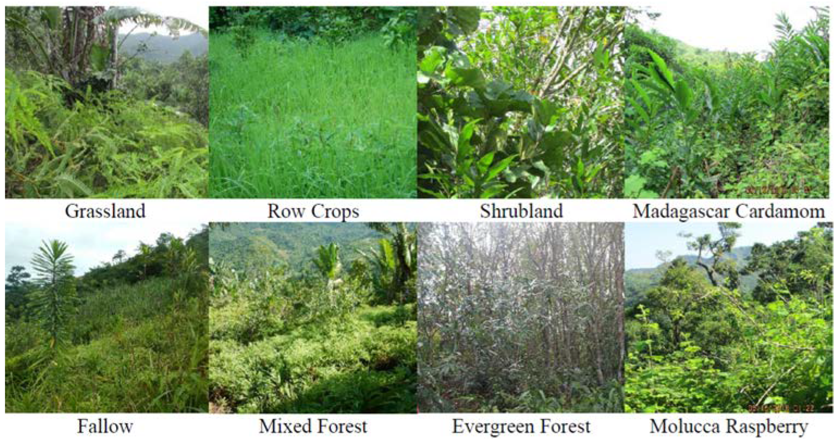
9]. Three habitat-altering invasive plant species seen prominently within the BNR are Molucca Raspberry (Rubus moluccanus), Madagascar Cardamom (Afromomum angustifolium), and Strawberry Guava (Psidium cattleianum) [10]. Although Madagascar Cardamom is native to Madagascar, its weedlike characteristics in degraded areas within and surrounding the BNR make it invasive in the region [11].
To effectively conserve biodiversity, an understanding of the human–environmental interactions is needed, since basic human needs have a direct impact on various conservation efforts through unsustainable agricultural practices, human encroachment, and bushmeat consumption [4,5]. Agriculture is the primary source of income for the locals around the BNR, with ‘tavy’, a cultural slash-and-burn system, being practiced by 80–85% of farmers [5,12]. To ensure a source of income, locals around the BNR amplify and expand agricultural production even if they are unable to sell their products to local markets [12]. The poorest households around the BNR spend two-thirds of their income on food [13] with many households experiencing chronic or temporary food insecurity, which is intensified by climate change-related events such as increased frequency of cyclones, causing flooding, landslides, and damage from powerful winds, accidents, illness, deaths, and animal and crop disease [12].
These human–environmental interactions are often studied by mapping the landscape with different land cover and land uses using Remote Sensing. In recent studies, remote sensing has been used to study the BNR and surrounding ecosystems [10,14] and the entire island of Madagascar [4], producing detailed Land Use or Land Cover maps through various methods [15]. Freely available imagery data from Landsat missions is a major data source for both large- and small-scale classification maps [15]. However, coarse resolution (10–100 m) images are not spatially detailed enough for forest conservation mapping projects [16] or the identification of individual tree species [17]. WorldView-3 (WV-3) has a high spatial resolution with a resolution of 1.2 m for visible bands (VNIR), 3.7 m for shortwave infrared (SWIR) bands, and 0.3 m in the panchromatic band. With the increased spatial resolution, pixel-based models that use only spectral information within each pixel for classification are not as effective as the within-class variation is much greater than the between-class variation. Classification accuracy is reduced, and maps derived from pixel-based methods show a salt-and-pepper effect when created based on spectral information alone using high-resolution imagery.
While the spatial and texture dimension of the remotely sensed imagery provides information regarding feature extent, the spectral data provide information that can be used to differentiate between classes [15]. The shortwave infrared (SWIR) bands within the WV-3 satellite provide added values for improved vegetation mapping. The SWIR bands can detect non-pigment biochemical constituents of plants including water, cellulose, and lignin [18]. SWIR-4 (1729.5 nm), SWIR-5 (2163.7 nm), and SWIR-8 (2329.2 nm) can detect characteristic absorption features of nitrogen, cellulose, and lignin, respectively [18]. The inclusion of SWIR bands for tree-species classification has been shown to increase the accuracy to varying degrees [18,19].
Support Vector Machines (SVM), Decision Trees (DT), Random Forests (RF), and Deep Neural Networks (DNN) have been used for image classification [15]. However, these methods are dependent on handcrafted features and require domain expertise [20]. Therefore, a shift is seen toward the use of deep learning algorithms for the creation of classification maps with Convolutional Neural Networks (CNNs) dominating because of their ability to extract relevant information automatically from imagery [20]. CNNs are a type of Deep Neural Network model architecture that can extract various features automatically and out-perform pixel-based machine learning models [19,20,21]. “Automated learning” here is the process in which a computer program is trained to learn and apply translationally invariant and spatially hierarchical patterns within the image through convolutional and pooling layers [20]. Well-known deep CNN architectures used for image classification problems include AlexNet [22], VGG Networks [23], ResNet [24], DenseNet [
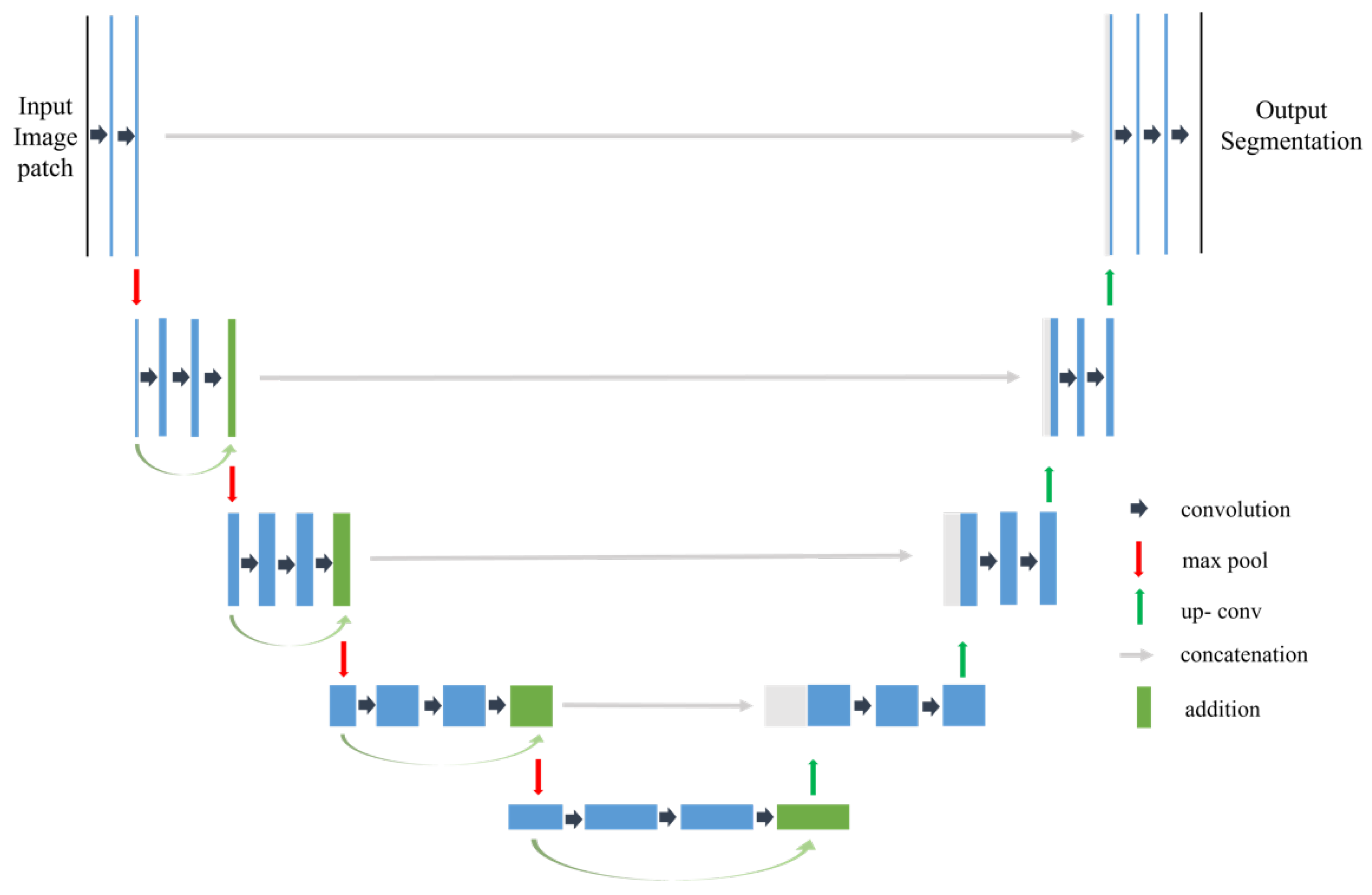
25], among others. However, the fully connected layers at the end of any CNN architecture do not preserve the 2D input image and predict a single class for each input image. For mapping purposes, a per-pixel prediction of the 2D input image is required. Thus, new methods were developed, such as Fully Convolutional Networks (FCNNs) [26] for image classification through pixel-wise semantic segmentation. Ref [26] defined an architecture that replaces the dense fully connected layers with a deconvolutional layer. This FCNN architecture can create pixel-based classifications or semantic segmentation of the input image. Segmentation and classification of the input image occurs through the FCNN architecture, resulting in an end-to-end classification map. The input to the model is a 2D image, which results in a classification based on both spectral and textural features. SegNet and U-Net are types of FCNN for per-pixel semantic segmentation of input images [27,28].
FCNNs and their variants have been used for end-to-end per-pixel image classification of high-resolution satellite images [29,30,31,32,33]. The number of classification classes varies with a maximum of 13 classes seen in [30]. For studies with more than 10 classes, high-resolution GaoFen-1, GaoFen-2, IKONOS, WV-2, and Quickbird satellite imagery were classified [29,30,32]. However, these studies that use fully convolutional networks focus on the classification of land covers for an urban landscape [29,32] and agricultural landscapes [30] with a few focusing on ecological landscapes [34].The importance of high spatial resolution (3.7 m) SWIR bands for image classification, especially forest cover classification, has been unknown because 3.7 m SWIR bands have not been previously available for commercial or academic research. To the authors’ best knowledge, FCNNs, that incorporate spatial features, have not been utilized for tropical forest cover mapping using raw WV-3 satellite imagery.
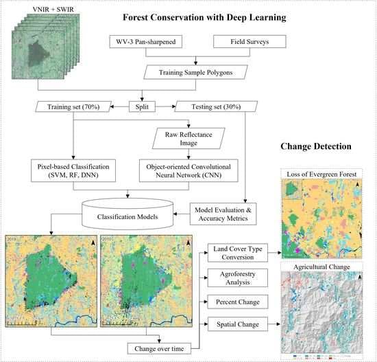
While considering the size of the BNR and more importantly, the rugged terrain, remotely sensed data is a top contender to map forest cover. It is hypothesized that (1) the end-to-end FCNN model (U-Net) will outperform other pixel-based methods (SVM, RF, DNN) due to the inclusion of textural features and end-to-end mapping capability, (2) the exclusion of SWIR bands would reduce the overall accuracy for all classification methods, with a greater reduction for SVM and RF, and (3) based on trends seen by [14], a negative human influence on the BNR and surrounding habitat is expected. The objectives are to (1) to develop an end-to-end automated deep learning model for forest cover mapping using WV-3 imagery, (2) to evaluate the influence of WV-3 SWIR bands for tropical forest cover mapping, and to evaluate the impact of conservation efforts in the region by international organizations by analyzing land cover change from 2010 to 2019.

2. Materials and Methods

2.1. Study Area

The 13 km × 13 km study area (Figure 1) is located approximately 40 km northwest of the coastal city of Toamasina and is centered over the BNR. The area is characterized by steep slopes varying from 0 to 55°, isolated forest patches, and extensive agriculture. There are 21 streams that flow through the BNR, and it represents an important watershed for the region that includes the headwaters for two major river systems. The region is characterized by a hot and humid climate with an annual rainfall of over 2000 mm and an average humidity ranging between 80% and 90%. The annual average temperature is 24 °C, with a low of 16 °C in the months of June through August and highs of 32 °C in the months of December through February [10].

2.2. Data

2.2.1. Ground Truth Data Collection

Ground truth data were surveyed in 2018 by a local field team facilitated by the Madagascar Fauna and Flora Group (MFG). For each surveyed location, the type of land cover, approximate surface area covered, and associated image was documented. Survey plots were selected such that the target land cover or land use class covered a large and homogenous area. Then, GPS data was recorded at least one location within or on the border of a plot, depending on accessibility. The size of the plots varied, based on the location. Then, these data were categorized into 11 classes (Figure 2; Table 1). These ground truth points were used as a reference to create samples for model training and testing.
The choice of classification scheme has implications on the map application, and different classification schemes are of value to different management groups. In this research, classes were defined according to land cover (4 classes) and forest cover type (7 classes). The description of each class is seen in Table 1.

2.2.2. Imagery Data

WorldView-3 imagery over the study area imaged on 19 February 2019 (Figure 1) with minimal cloud cover was acquired. The data were atmospherically and radiometrically corrected [35,36,37] and orthorectified by the vendor, Maxar Technologies [38]. The WorldView-3 data contain 8 bands in the visible (400–1040 nm with a spatial resolution of 1.2 m) and 8 bands in the shortwave infrared (1210–2365 nm with a spatial resolution of 3.7 m). Then, the imagery was stacked and resampled to a 1.2 m spatial resolution using the nearest neighbor resampling method with ENVI 5.4.1 software package (ENVI® image processing and analysis software, from Exelis Visual Information Solutions). Resampling of the SWIR data from 3.7 m to 1.2 m was necessary to analyze the data at a uniform spatial resolution.

2.2.3. Training Samples

Sample polygons were generated such that only pure pixels were selected, using the ground truth data as a reference. Polygons were created with the survey points projected to 0.31 m GSD WorldView-3 pan-sharpened visual imagery, ensuring that only homogenous polygons were digitized using the GPS recordings. Additional training samples were created through photointerpretation to create a total of 360 polygons spread out over the entire study area. To compare results from multiple models, the same training and testing data were used for all classification models. Thus, once the sample polygons were created, it was split into training (70%) and testing (30%). The ground truth data, imagery, model training data, and model testing data were georeferenced to the Universal Transverse Mercator (UTM) coordinate system, zone 39 South with the World Geodetic System Datum of 1984 (WGS 84).

2.3. U-Net

A typical Convolutional Neural Network (CNN) contains a convolutional layer and a pooling layer. In the convolutional layer, a filter of size N × N pixels slides over the input image and performs element-wise multiplication to produce a single value. The filter slides right to left and downward bottom to repeat the element-wise multiplication, resulting in a feature map with a shape reduced by a value of N-2. The pooling layers aim to reduce all the useful information extracted from convolutional layers to much smaller dimensions. CNNs have been used for imagery-based applications because of their ability to extract spectral and textural information from the images [20]. Textual information derived from convoluting kernels in the neural network enhances the existing spectral information. In a Fully Convolutional Neural Network (FCNN), the final fully connected dense layer within a CNN architecture is replaced with an up-sampling convolutional network. The architecture of the U-Net model (Figure 3) first implemented by [27] for biomedical image segmentation has been used in forest type and tree species mapping [17] as well as the delineation of human-induced deforestation [16].
The U-Net algorithm [27] is a type of FCNN where the encoding path follows the standard ResNet CNN structure: repeated 3 × 3 unpadded convolutions with ReLU as activation functions and standard 2 × 2 max pooling operations with different numbers of kernels. However, the decoding path replaces max pooling operations with transpose convolutions, which doubles the resolution of each feature map. In addition, each up-sampled feature map is concatenated with cropped feature maps from the “same level” of the encoding path. This enables the precise localization and compensates for the loss of information in the pooling layers. As a result of this, the U-Net architecture was used over other FCNNs. The final layer of U-Net is 1 × 1 convolution with softmax activation, which produces a per-pixel segmentation map for the image.
The quantity of training data derived from ground data collection in 2018 was limited. A U-Net implemented with Keras produced a low training and testing accuracy with segmentation results on testing data differing between repetitions. Implementing a U-Net model within the arcgis.learn module of the ArcGIS API for Python [39] removed the requirement for a quantitatively massive dataset. Additionally, the U-Net implemented through argis.learn is pretrained on ImageNet to further improve classification accuracies. This reduces the time and resources spent on ground truth data collection. Hyperparameter tuning was done to select the best U-Net model [31,34,40]. Based on hyperparameter optimization, it was found that the best model uses an input patch size of 64 × 64 pixels and a ResNet-50 backbone [31,34,40].

2.4. Support Vector Machine (SVM)

Support Vector Machine (SVM) is a non-parametric method that attempts to classify non-linearly separable data through the kernel trick in which input data are mapped to a higher-dimensional feature space where a linear decision plane can be easily computed to separate the classes [41]. This hyperplane is drawn such that the distance between the nearest data vectors and the hyperplane is maximized. The SVM model was created using the sklearn module (scikit-learn 0.24).
The accuracy of the SVM model is dependent on the choice of kernel, and a radial bias kernel is shown to outperform other kernels for remote sensing applications [42]. The RBF kernel requires tuning of two parameters—C and γ. Choice of the C parameter involves a trade-off between correct classification and maximization of the margin. Thus, a smaller C value will result in a wider margin and thus a lower accuracy. The γ value controls the radius of influence of the training samples. Thus, a greater value will result in a model that overfits on the training data and poor generalization on the testing data. The best values for C and γ were optimized using GridSearchCV (scikit-learn 0.24) and were found to be 1000 and 1, respectively.

2.5. Random Forest (RF)

The RF algorithm constructs multiple decision trees (DTs), or classifiers, that each predict a class [43]. Each tree within the RF is created using different training data subsets, which are selected through repetition and replacement of the original training dataset. This repetition and replacement create a ‘bagged’ dataset for each of the decision trees within the random forest. The samples that are out of the bag, the so-called out-of-bag samples (OOB), are used for validation of the RF model. The final prediction of the RF is based on the majority vote from all trees. The RF model was created using the sklearn module (scikit-learn 0.24). The number of trees and the maximum number of features to be considered for the best split were tuned via GridSearchCV (scikit-learn 0.24) and were found to be as follows: best number of trees = 130; maximum features required for split = auto.

2.6. Deep Neural Network

A Deep Neural Network (DNN) consists of multiple hidden layers, made up of ‘n’ number of neurons. These neurons are interconnected with neurons of the preceding and next layer, through some weight (m) and bias (c), such that,
y = mx + c
The network attempts to learn the values for the various weights and biases, the parameters of the model, by minimizing the cost function. The choice of the cost function is important, as this function guides the model in the direction of the correct weights and biases for accurate predictions. The cross-entropy loss function is used for the DNN model.
The number of neurons and the number of hidden layers all affect the predicting power of the network. Thus, these parameters were adjusted, resulting in the architecture seen in Figure 4. The presence of a dropout layer, with a value of 0.23, after hidden layer 5 and a batch normalization layer after hidden layer 2 increased the testing accuracy of the model. These additional layers—dropout and batch normalization—reduce the over-fitting of the model on the training data and increase generalization on testing data. The hyperparameters in this network—the learning rate, number of epochs, and batch size—were further tuned such that the testing accuracy and the kappa were the best among all models. The optimized hyperparameter values for learning rate and batch size were 0.007 and 48, respectively.

2.7. Accuracy Assessment

To compare the accuracy of various models independent testing data, i.e., same for all models, is used for model evaluation. The confusion/error matrix and subsequent metrics are calculated on a pixel-level basis. This confusion matrix shows the model prediction of each class (rows) compared to the original class (columns) as defined by the testing data. The quantitative evaluation was conducted by using overall accuracy (OA), kappa coefficient, user’s accuracy, producer’s accuracy, and F1 scores, which were derived using the error matrix.
The OA is defined as the ratio of the number of correctly classified samples to the total number of test samples (Equation (2)). While OA measures simple percentage agreement, the Kappa coefficient measures the degree of agreement by considering the correctly classified samples that may happen by chance and is usually less than or equal to 1 (perfect agreement) (Equation (3)).
O A = T P + T N T P + T N + F P + F N
k a p p a   c o e f f i c i e n t = P o P e 1 P e
where P o : Observed Accuracy & P e : Accuracy obtained by chance.
Producer’s accuracy measures the accuracy of model predictions, while user’s accuracy measures whether the predictions reflect true ground cover (Equations (4) and (5)). These values for producer’s and user’s Accuracy—TP, FP, and FN—are based on an error matrix that is weighted according to the proportion of area in each cell of the matrix [44]. The F1 score is mathematically defined in Equation (6).
True Positive (TP) is the number of pixels for a class correctly predicted by the model. False Negative (FN) is the number of pixels for a certain class wrongly predicted as another class, while False Positive (FP) counts the number of pixels predicted as a certain class that actually belong to another class.
P r o d u c e r s   a c c u r a c y = T P T P + F N
U s e r s   A c c u r a c y = T P   T P + F P
F 1   s c o r e = 2   T P 2   T P + F P + F N

2.8. Land Cover and Land Use Change

Conservation efforts were quantified by investigating the land cover and land use change over time. Since the types of land cover classes studied here were the same as the 2010 classification [10], the map created here was compared with one created by [10]. Since the 2019 imagery covered a much larger extent than the 2010 classification product, the change metrics were based on the 2010 imagery extent. Zone of protection (ZOP) is defined as a 100 m wide ecotone at the perimeter of the BNR, which extends 100 m outside the boundary of the BNR [14]. The activities within the ZOP have an impact on flora and fauna within the BNR due to the forest edge effect, since both human and ecological activities overlap in the ZOP. Therefore, change metrics for ZOP were computed for an area that extends 100 m inward and outward from the boundary. In other words, the statistics of the changes for the ZOP include 100 m within the BNR plus the ZOP, which extends 100 m from the boundary outside the reserve. The overall percent change for each land cover and land use was calculated by dividing the difference between 2019 and 2010 total area by the total area in 2010 for that specific land cover and land use; see Equation (7).
P e r c e n t   C h a n g e =   2019   a r e a 2010   a r e a 2010   a r e a ×   100
In order to visualize the trajectory of change spatially, we used a grid cell approach as in [45]. A grid cell size of 10 × 10 m was used to aggregate pixel-level land cover and land use types. We chose this grid size as it is approximately the size of mature trees so that we can track the changes to the scale of individual trees. The percent change was computed based on aggregated percent land cover and land use type within each grid cell using a combination of ArcGIS processing tools and python code. First, a 10 m fishnet grid was created using ArcGIS Pro, which was intersected with 2010 and 2019 classification shapefiles. Then, polygons of the same class that intersect (fall within) a fishnet grid were aggregated to produce the sum of each unique land cover within the fishnet cell (using ArcGIS Pro ‘Summarize Attributes’ tool). This resulted in a table with multiple rows with the various land cover types in the same column. In order to organize each land cover percentage in separate columns (which is needed to calculate spatio-temporal change), the table was pivoted (using ArcGIS Pro “Pivot” tool) such that each grid cell has the total percentage of a specific land cover organized by a table of columns. Finally, the percent area of a specific land cover per grid cell was calculated, and the percent change was computed as the difference between 2010 and 2019 classification products.

3. Results

3.1. Classification Results

The U-Net model produced a 90.9% accuracy, outperforming other pixel-based models (Table 2). The SVM, RF, and DNN models produced an overall accuracy of 88.6%, 84.8%, and 86.6% respectively. Among SVM, RF, and DNN models, SVM was able to better distinguish between the classes.
The U-Net model provided the highest producer’s and user’s accuracy for Mixed Forest and Evergreen Forest. The producer’s and user’s accuracy for Molucca Raspberry was greater than 95% for all methods, with the DNN model providing the highest accuracies and U-Net providing the lowest accuracies. Although the U-Net model produces the highest producer’s accuracy of 81.6% for Madagascar Cardamom, only 84.5% is actually Madagascar Cardamom. An increase in both the producer’s and user’s accuracy was seen for the U-Net model for Guava. The producer’s accuracy for Shrubland is seen to increase for the U-Net model, while the user’s accuracy decreased. The U-Net model resulted in the highest user’s accuracy and the lowest producer’s accuracy for Grassland compared to other methods, while the SVM model produced the best producer’s and user’s accuracy for Grassland. Open Water, due to its unique spectra compared to other classes, results in 100% user’s and producer’s accuracy across all models. The U-Net model resulted in 100% producer’s and user’s accuracy for the Residential and Fallow classes. As shown in Figure 5, the F1 score from U-Net is the highest for all classes considered, indicating that U-Net is a better model overall for tropical forest habitat mapping.

3.2. SWIR Bands

The removal of SWIR bands reduced the accuracy by 5.42%, 3.18%, 8.55%, and 1.87% for the SVM, RF, DNN, and U-Net models, respectively (Table 3). The confusion matrix for the DNN and U-Net models from which accuracy metrics are derived is shown in Figure 6. The DNN model is chosen for comparison because of the greatest percent change due to the removal of SWIR bands, producing the worst accuracy when SWIR bands were removed. The U-Net model is chosen because of the lowest reduction in accuracy when the SWIR bands were removed. The removal of the SWIR bands amplifies the number of misclassified pixels between classes: for example, guava pixels being classified as Madagascar Cardamom (Figure 6). A decrease in the producer’s and user’s accuracy for Madagascar Cardamom and Guava, which are invasive plant species, is seen (Figure 7).

3.3. Spatial Distribution of LCLU

A LCLU map was created through post-classification editing of the best model (U-Net) results to further reduce the errors in an effort to create a “gold standard” classified map (Figure 8) by further removing spurious pixels and majority analyses. Each pixel within the map was manually scanned for misclassified pixels using photointerpretation of the 0.31 m GSD pan-sharpened image, and such pixels were reclassified using the ‘Pixel Editor’ tool in ArcGIS Pro. This map accurately describes the class of each 1.2 m × 1.2 m pixel within the map. Based on Figure 8, around 50% of the study area is covered by shrubland, 33% is covered by mixed and evergreen forests, and 4.7% is covered by invasive plant species. Another 8% of the study area is used for cultivation (Row Crops and Fallow). The detailed distribution in percent of the total study area is shown in Table 4.

3.4. Land Cover and Land Use Change Analysis

3.4.1. Change in the Study Area

The quantitative change was conducted for the overlapping extent (Figure 9) between the two classification maps produced for 2010 and 2019 (Table 5). An increase is seen for the following classes: Evergreen Forest (1.5%), Mixed Forest (4.9%), Residential (44.3%), Shrubland (37.2%), Open Water (53.6%), and Madagascar Cardamom (47.5%); a decrease is seen for the following classes: Molucca Raspberry (−55.7%), Row Crops (−56.1%), Fallow (−31.0%), Grassland (−63.4%), and Guava (−6.1%).
The 44% increase in Open Water is attributed to the extensive mapping of the streams in the study area as well as increased panchromatic resolution of 0.3m that enabled the discernment of very narrow streams, which is not possible with the 4 m spatial resolution of IKONOS data used in the 2010 classification. Since the area represents an important watershed for the region, mapping all the streams within the area is important to guide decision-makers and conservationists.
With the increasing population, an increase in Residential land use is seen within the study area. This is seen both in the increase in the spatial extent of residential areas as well as the emergence of new hamlets (Figure 10). Furthermore, the increased spatial resolution of the 2019 imagery (from 4 m to 1.2 m) has resulted in the identification of isolated huts believed to be seasonal agricultural homes called lasy. Its isolated nature along with the near distance to the agricultural fields validates this hypothesis.
It should be noted that trees within the boundaries of residential areas, originally classified as Mixed Forests, were re-classified as Residential in this study to quantify the change in residential tree cover for agroforestry analysis. Based on the re-classified pixels, tree cover within residential areas was estimated for 2010 and 2019 (Figure 11). A 32% increase in the tree cover in residential areas was observed in 2019, which may be associated with tree growth and increased fruit tree plantation within residential areas encouraged by conservation groups and local authorities to combat food insecurity.
The reduced area for Row Crops and Fallow is seen primarily within the ZOP. It can potentially be attributed to a seasonal shift in agriculture. The imagery from which the 2010 classification map was derived was collected in May, while the current imagery was collected in February. Additionally, the replanting of native flora in the ZOP to protect the degradation of evergreen forest at the forest edges is also a major factor in the reduction of agriculture in the ZOP.
The classes that were converted to Shrubland in 2019 are shown in Figure 12. The conversion of 2010 Evergreen Forest to Shrubland areas in 2019 is considered as land degradation and is seen in forest fragments within the study area, east of the BNR (Figure 13). Around 70% of the conversion was seen from Fallow and Grasslands to Shrubland. The vegetation in these areas could be late inter-cropping periods when agricultural fields have been left fallow for several years, or it could be the early stages of a Mixed Forest or regenerating Evergreen Forest, but the small height of these trees has resulted in a Shrubland classification.

3.4.2. Change within the BNR

The land cover changes within the BNR are shown in Table 6. Increases within Mixed Forest and Evergreen Forest are observed while decreases in invasive plant species are observed within the BNR (Figure 9; Table 6). The classes that were converted to Mixed Forest in 2019 are shown in Figure 14. When comparing land cover in 2010 and 2019, 3080 ha, 3101 ha, and 459 ha of invasive Molucca Raspberry, Madagascar Cardamom, and Guava respectively were converted to Mixed Forest in 2019 probably due to tree growth. However, 876 ha of Evergreen Forest were also converted to Mixed Forest in 2019.

3.4.3. Change within the Zone of Protection (ZOP)

The ZOP, also called the buffer zone, acts as a transition between protected areas and surrounding unmanaged landscape that reduces the negative impacts on protected areas. In this zone, human and ecological activities clash. In the ZOP, while the extent of invasive Molucca Raspberry has decreased over time, an increase in the extent of Madagascar Cardamom and Guava is observed (Figure 15; Table 7). Within the ZOP, anthropogenic land use (i.e., residential) decreased by 17.9%, and Row Crops and Fallow areas decreased by a 76% and 4%, respectively. The decrease in anthropogenic land use is complemented by an increase in the extent of Mixed and Evergreen Forests. Detailed mapping of streams, which can be seen in Figure 15, accounts for the 430% increase in Open Water. It must be noted that this significant increase in Open Water class was the result of the super-high resolution of the 2019 WV-3 imagery compared to the IKONOS imagery used in 2010, which allowed better discrimination of smaller streams or streams that are covered by trees.

4. Discussion

4.1. Land Cover and Land Use Classification

Only spectral information is used as input features for classification using SVM, RF, and DNN. Although classification accuracies are greater than 80% for all models, a salt-and-pepper effect is seen in the classification maps (Figure 16), which is common for pixel-based classification with very high-resolution satellite data. Note that the SVM classification map is shown here because of its higher accuracy compared to RF and DNN models. With very high-resolution images such as WV-3, the increased spatial resolution results in an increase in the within-class variation and a decrease in the between-class variation, decreasing the separability between classes [46]. This can be observed in the confusion matrix with higher percentages of misclassified pixels (Figure 6). Additionally, as seen in Figure 17, all forest covers have similar-looking spectral curves. To reduce these misclassified pixels, researchers have used vegetation indices and textural features such as the Gray Level Co-occurrence Matrix (GLCM) [46]. However, the creation of such handcrafted features is time consuming, requires tuning, and needs domain expertise, highlighting the advantage of end-to-end CNN-based classification that utilizes texture information through an FCNN architecture.
The FCNN U-Net model produced an overall accuracy of 90.9%, outperforming the other pixel-based models studied here. Similarly, U-Net has outperformed other pixel-based models in other studies [40]. The improvement in accuracy can be attributed to the architecture, which is common within all FCNN encoder–decoder type models. Firstly, the 2D kernels within convolutional layers consider spatial information. The convolutional layers extract hierarchical features, and therefore, raw WV-3 imagery input alone is able to produce >90% accuracies [17]. Finally, the fully convolutional nature can segment and classify each pixel in the input image resulting in an end-to-end classification map [26,30,40]. Thus, semantic segmentation at the pixel level along with the extraction of features through convolutional layers and the inclusion of spatial information results in the higher accuracy of the FCNN-based U-Net over other pixel-based models. However, one disadvantage of the U-Net model is the labeling of each pixel in the training data. Abundant data are needed for training deep neural networks of at least 1000 image samples. In such cases, a pretrained network can reduce the amount of training data needed [47]. The U-Net implemented within arcgis.learn had a ResNet-50 backbone that was pretrained on ImageNet.
The following classes provided a higher user’s accuracy and producer’s accuracy across all pixel-based models: Open Water, Molucca Raspberry, and Row Crops. These classes have unique spectral signatures that enable the separation of each class from other classes (Figure 17). SVM, RF, and DNN models in this study suffer from misclassified Fallow (bare land) and Residential (built-up) pixels because of similar reflectance curves (Figure 17). The misclassification can be reduced by using an FCNN-based U-Net model that includes textural features (Table 2, Figure 5) [30]. A lot of misclassified pixels are seen between forest covers—namely, Mixed Forest, Evergreen Forest, and Guava [48]. Training data for Mixed Forest were created based on limited ground reference data points. Misclassified pixels among these three classes—Mixed Forest, Evergreen Forest, and Guava—could stem from inconsistent training data. The training data might not have been able to capture the spectral variability within each class, which could have reduced the separability between the classes. The spectral signature of Guava is difficult to recognize even with using other sources of data [10]. Furthermore, guava does not need direct sunlight and therefore grows beneath the forest canopy which makes its identification through satellite imagery challenging. The producer’s and user’s accuracy decreased for Madagascar Cardamom and Molucca Raspberry using the U-Net model. This decreased accuracy may be due to the limited training samples for the U-Net model implemented. Deep architectures usually require thousands of training data so that the model is able to generalize on the testing data. The samples were limited, and images were rotated to increase the training and testing data.

4.2. Contribution of SWIR Bands

WV-3 SWIR bands can detect non-vegetative pigments [18], and thus, the removal of these bands reduced the overall accuracy by 5.42%, 3.18%, 8.55%, and 1.87% for SVM, RF, DNN, and U-Net models, respectively (Table 3). Therefore, the inclusion of WV-3 SWIR bands improves the separability between vegetative classes and improves classification accuracy.
Since the RF, SVM, and DNN models use only the spectral features for classification, the removal of SWIR bands has a greater impact on the overall accuracy. Based on the percent decrease in accuracy, the SWIR bands were most useful in separating classes in the DNN model, followed by the SVM and RF models. Within U-Net, the inclusion of spatial/textural features results in only a 1.87% decrease in accuracy when SWIR bands were excluded, confirming that CNN-based approaches can provide robust and accurate results just with VNIR data, excluding the need for expansive SWIR data collection. However, it is worth noting that we used a 2D CNN architecture in this paper. A 3D CNN architecture that fully utilizes spectral differences among classes along with texture and patterns may show the benefit of SWIR bands differently.
WV-3 VNIR and SWIR bands have been used to discriminate between tree species [18,19] and crop types [49]. These studies showed that the contribution of each SWIR bands is class-specific and varied for different land cover and land use types, which was further confirmed by this study. A decrease is observed in the F1 score of Mixed Forest, Fallow, Open Water, and Guava when SWIR bands were removed across all classification methods employed. For the remaining classes, an increase in the F1 score is seen for at least one classification method.
The F1 scores for all classification methods and selected land cover classes are shown in Figure 18 Guava is highlighted in Figure 18a, because of the highest decrease in F1 score for SVM, RF, and DNN models compared to all other classes. For the U-Net model, the removal of SWIR bands reduced the F1 score by almost 50% for Madagascar Cardamom (Figure 18b). In Figure 18c, Evergreen Forest is highlighted for 16 (VNIR + SWIR) bands and eight (VNIR) bands as the F1 score increased for RF and U-Net models upon removing SWIR bands. Figure 18d shows the decrease in F1 score for Mixed Forest without SWIR bands; similarly, in Figure 18e, decreases are evident for Molucca Raspberry. For Row Crops and Residential, the F1 score slightly increased when SWIR bands were removed for both RF and DNN, respectively. This increase could be attributed to the fact that both Row Crops and Residential land use are best differentiated by VNIR bands and the relatively lower resolution of SWIR may have affected the metric. For Fallow, as shown in Figure 18h, a decrease is evident when SWIR bands are removed, indicating the importance of SWIR bands for identifying Fallow, as SWIR regions are most effective for mapping crop residue in Fallow. Finally, for Shrubland (Figure 18i) and Grassland (Figure 18j), SVM, RF, and DNN were unable to identify the class without the presence of SWIR bands, producing a percent decrease in F1 scores, while the U-Net model was able to produce better F1 scores when the SWIR bands were removed.

4.3. Accuracy of Classification Maps

Land cover and land use maps are highly advantageous to conservationists and land managers for the establishment of new conservation programs, for quantitative evaluation of various existing conservation programs, and for the estimation of forest fragmentation rates [4,16]. Moreover, it is beneficial to users that these land cover maps are 100% accurate.
Accuracy estimation for each pixel in classification maps is not possible, since ground truth data are not available for each pixel. Therefore, the accuracy of classification maps is calculated based on pixels that are representative of the image [50]. These pixels are taken at random and are not used to train the classification model. If the sample pixels selected are not true representations of the study area, the resulting map accuracy will be inaccurate [50], and these accuracy values should be treated with caution.
To increase the accuracy of land cover maps created through classification, the maps can be inspected and subsequently edited. Although such a process is labor-intensive and time consuming, it ensures a near 100% accuracy of the land cover map. Therefore, the final classified map was manually inspected, fine-tuned, and edited to reflect true land covers. For example, trees within the Mixed Forest class that obstruct rivers and streams are reclassified as Open Water. Other edits included the re-classification of misclassified Fallow pixels to Residential and vice versa. The land cover map was edited to correctly reflect the distribution of Madagascar Cardamom and Molucca Raspberry. The outcome of this post-editing as mentioned in previous sections is a gold standard map of the entire study area. Confusion matrices were computed by comparing the gold standard map and the LCLU maps produced by the machine learning algorithms including the U-Net and SVM models (Table 8).
Although the overall accuracy of the U-Net model based on testing data of limited random pixels is over 90%, the accuracy based on the gold standard map is only 77%, which reflects the accuracy over the entire study, including all pixels in the imagery as opposed to the testing accuracy based on the limited testing pixels. Similarly, a much lower accuracy is seen with the SVM model. There are numerous reasons for the resulting low accuracy for the U-Net model, which can be attributed to the training of the models themselves. With additional training data, the spectral variation within each class (Figure 17) could be learned to better predict the land cover. Another source of error for the lower accuracy (Table 8) is Open Water. Although the overhead imagery shows tree cover above a stream, these tree pixels over water features are reclassified to Open Water in the gold standard map. Since the area represents an important watershed for the region, accurate mapping of these streams is important. Similarly, landslides expose bare rock, and their spectral signature is very similar to that of the Fallow class. Thus, both models classify those exposed rocks as Fallow. Although this classification is ‘spectrally’ accurate, it is not reflective of the true LCLU. Additionally, the low accuracy of 66% for the SVM model can be attributed to the salt-and-pepper effects of pixel-based classification.

4.4. Conservation Efforts in the BNR

Ref [14] found, based on imagery acquired in 2010, that 81% of the BNR consists of undisturbed and/or degraded evergreen forest, and 10% of the BNR consists of regenerating or degraded mixed forest. Results from the 2019 imagery show a 12.5% increase in regenerating Mixed Forest and a 0.7% increase in Evergreen Forest (Table 6). The regeneration of Evergreen Forest is a lengthy process, and therefore, the success of the restoration work within BNR is only slightly apparent with a 0.7% increase in Evergreen Forest. However, given that the trend in 2010 was toward increasing deforestation and forest fragmentation [14], this is already a worthwhile result, especially when coupled with a 13% and 28% increase in Mixed Forest in the BNR and the ZOP, respectively.
The Madagascar Flora and Fauna Group (MFG), an association of zoos and botanical gardens, manages the BNR in collaboration with the Madagascar National Parks (MNP) [12]. Since 2007, the MFG has run a community-based native forest restoration project in the BNR’s ZOP, a 100 m buffer extending out from the BNR, in partnership with the Madagascar National Parks. Another initiative is the control of invasive Guava in the BNR as well as the control of local invasive plants Madagascar Cardamom and invasive Molucca Raspberry, both of which have contributed to the 0.7% increase in Evergreen Forest in the BNR.
Knowing where and which LCLU types have been converted to Shrubland (Figure 12) within the study area is very valuable to the MFG and their partners at the MNP. This knowledge targets awareness raising and conservation efforts in areas of particular concern for example, the deforestation of formerly evergreen forests that are mainly remnant “Classified Forests”. These “Classified Forests” have a legally protected status but little practical protection. Similarly, knowledge of which classes were converted to Mixed Forest in 2019 in BNR (Figure 14) is also beneficial. For instance, although the conversion of Evergreen Forest to Mixed Forest amounted to 876 ha, the majority of classes that was converted to Mixed Forest was Molucca Raspberry (3080 ha), Fallow (2648 ha), Madagascar Cardamom (3102 ha), and Grassland (2697 ha).
Land use in the vicinity of protected areas is seen to negatively affect conservation efforts [51]. Since human and ecological activities overlap in these areas, the land cover changes are studied in the ZOP. The size of this transition zone is further dependent on the ecological, socio-economic, and hydrological interactions with the surrounding landscape [51], and therefore, it differs between protected areas. For the BNR, the size of this zone is taken as 100 m extending out from the BNR boundary. In the ZOP and 100 m within the BNR boundary, a decrease in anthropogenic land use is observed (residential areas, agricultural fields, and fallow land), which is complemented by an increase in mixed and evergreen forests (Table 7; Figure 19). These results are most likely a direct consequence of the MFG’s native forest restoration program and increased awareness-raising and lobbying by the MFG and Madagascar National Parks to discourage slash-and-burn agriculture in the ZOP. More recently, the MFG has initiated two efforts to reduce forest loss and promote more sustainable agriculture: the promotion of agroforestry and the distribution of fuel-efficient stoves.
Agroforestry around villages has been promoted by the MFG and their agroecology specialists since 2005. A 32% increase is seen in tree cover within residential areas (Figure 11), and it is found that there is an average of 6.5 species found in residential home gardens [12]. The increase in tree cover is indicative of native trees maturing over time and is also indicative of successful agroforestry efforts. The local population has already been practicing agroforestry for many generations, so it is not possible to quantify the impact due to the MFG’s specific efforts. However, the provision of training, trees and equipment since 2005 seems to be making a positive difference to tree cover in residential areas despite the overall growth of many of the residential areas. Ref. [12] also found that local farmers around the BNR are willing to increase tree crop production.
Ref. [5] found that 96% of the local population relies on firewood for cooking. To reduce the need for wood for firewood production, 2100 fuel-efficient stoves were distributed in 12 villages around the BNR. Distributions were made during three time periods: September 2018, May 2019, and September 2020. Prior to the collection of the imagery used for this analysis, 700 stoves were distributed. The change that occurred in this period (September 2018 to February 2019) is too short compared to the months where these stoves were not being used to assess their impact. In addition, trees are not generally felled completely for firewood but rather coppiced, or deadwood is collected below the forest canopy. Therefore, it would be almost impossible to quantify the impacts of fuel-efficient stoves through remote sensing techniques.

4.5. Human Geography Implications

Since agriculture is the main source of income for the locals [5,12], the mapping of agricultural land becomes important. In 2019, 5147 ha (3.08%) (Table 4) of the study area accounts for agricultural cover, which is associated with human settlements that account for 650 ha (0.38%) of the study area. The presence of these agricultural fields in the ZOP (Figure 15; Table 7) leads to an increase in human interaction in the buffer zone, which often has negative impacts on the biodiversity within the BNR. These agricultural fields are spread out over the study area, but a higher concentration is seen in the southern part, close to residential areas.
Figure 19 shows the comparison between percent changes in Evergreen Forest (Figure 19a) and percent changes in Agriculture (Figure 19b), highlighting the human impact (or lack thereof) on the BNR. Increases are seen in the Evergreen Forest within the BNR and surroundings and even the ZOP (outer edge of the gray polygon). Comparatively, decreases are seen in agricultural fields in the ZOP and other areas surrounding the BNR. These changes can be attributed to the fallow species succession and fallow/cropping regimes over 9 years. The fallow species succession can be used to either a forest restorative path or a forest degradative path. The land can be restored back to a forest from the regeneration of a shrub fallow. However, if the shrub fallow is cultivated it develops into a herbaceous fallow. The forest can still be restored at this stage; however, if it is further cultivated, it develops into grasslands whereupon if cultivated, it has low productivity. For a more detailed explanation of fallow species succession and ‘restoration’ or ‘degradation’ pathways, the reader is advised to read [52].
Locals around the BNR face food insecurity because of the growing population, which is based on the increased residential land cover (Table 4) and decreasing agricultural yields [12] in the study area. This food insecurity is further driving the forest cover conversion to agricultural fields. Food insecurity leads to the consumption of livestock (chickens, ducks, etc.) and to the consumption of wildlife—particularly lemurs [5,12]. Children around the BNR are reported to becoming weak, falling ill, and even performing poorly in school because of hunger [13]. Health care services are poor, costly, and inaccessible to locals around the BNR. It was common for locals to use medicinal plants as a cheaper option [13]. Therefore, although the conservation of species is important, it is also necessary to consider the needs of the local population. Future conservation efforts by the MFG include improving human health and recognizing the importance of people-oriented strategies in order to provide cash crops and a sustainable food source for the locals [13].

5. Conclusions

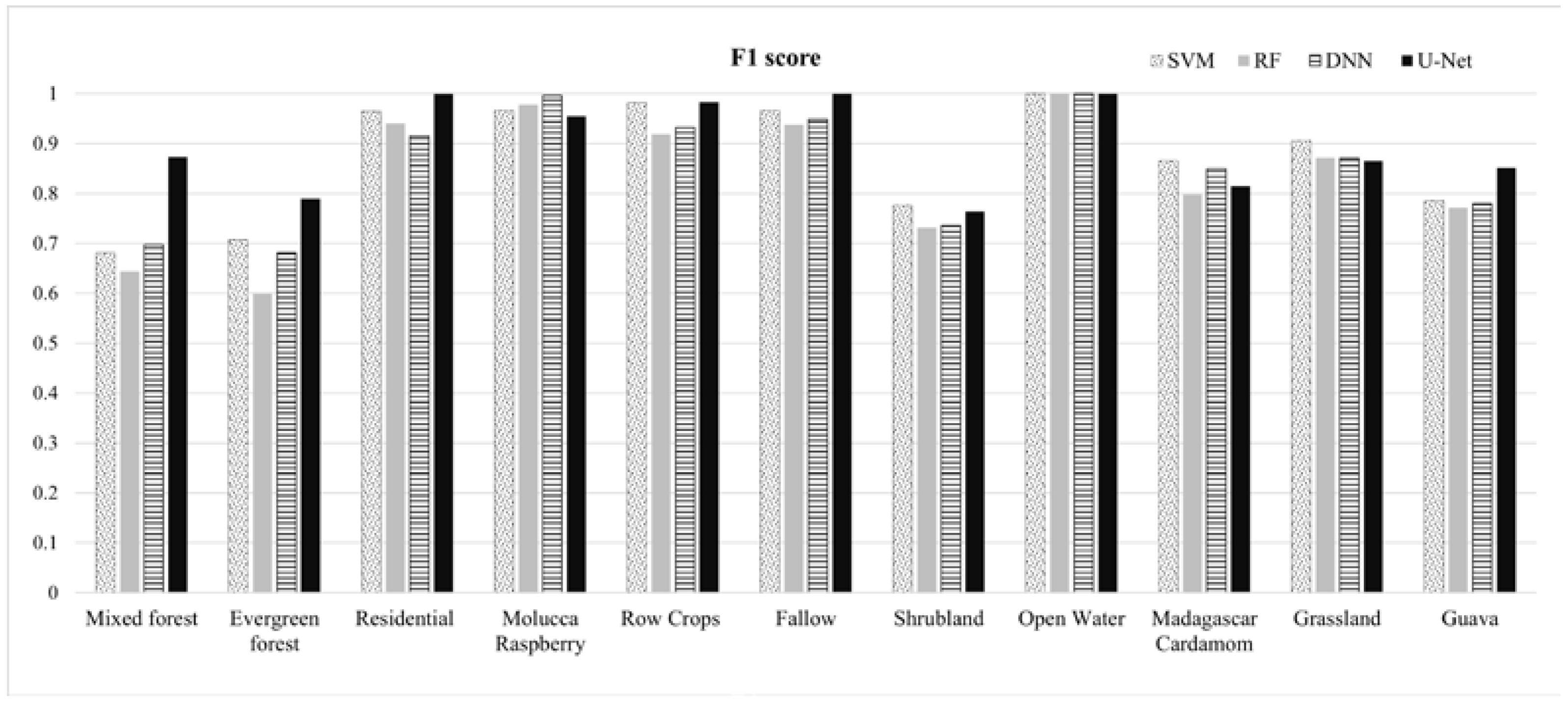
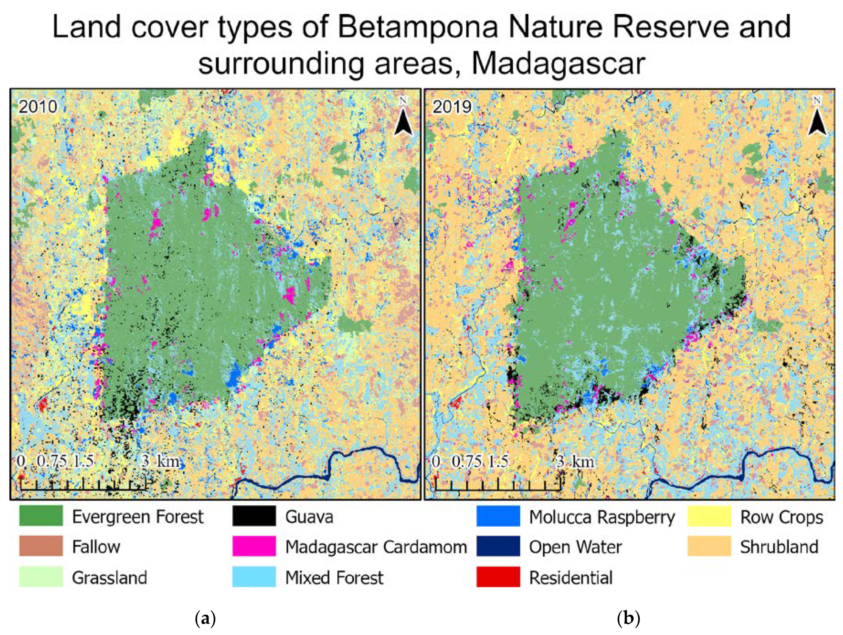
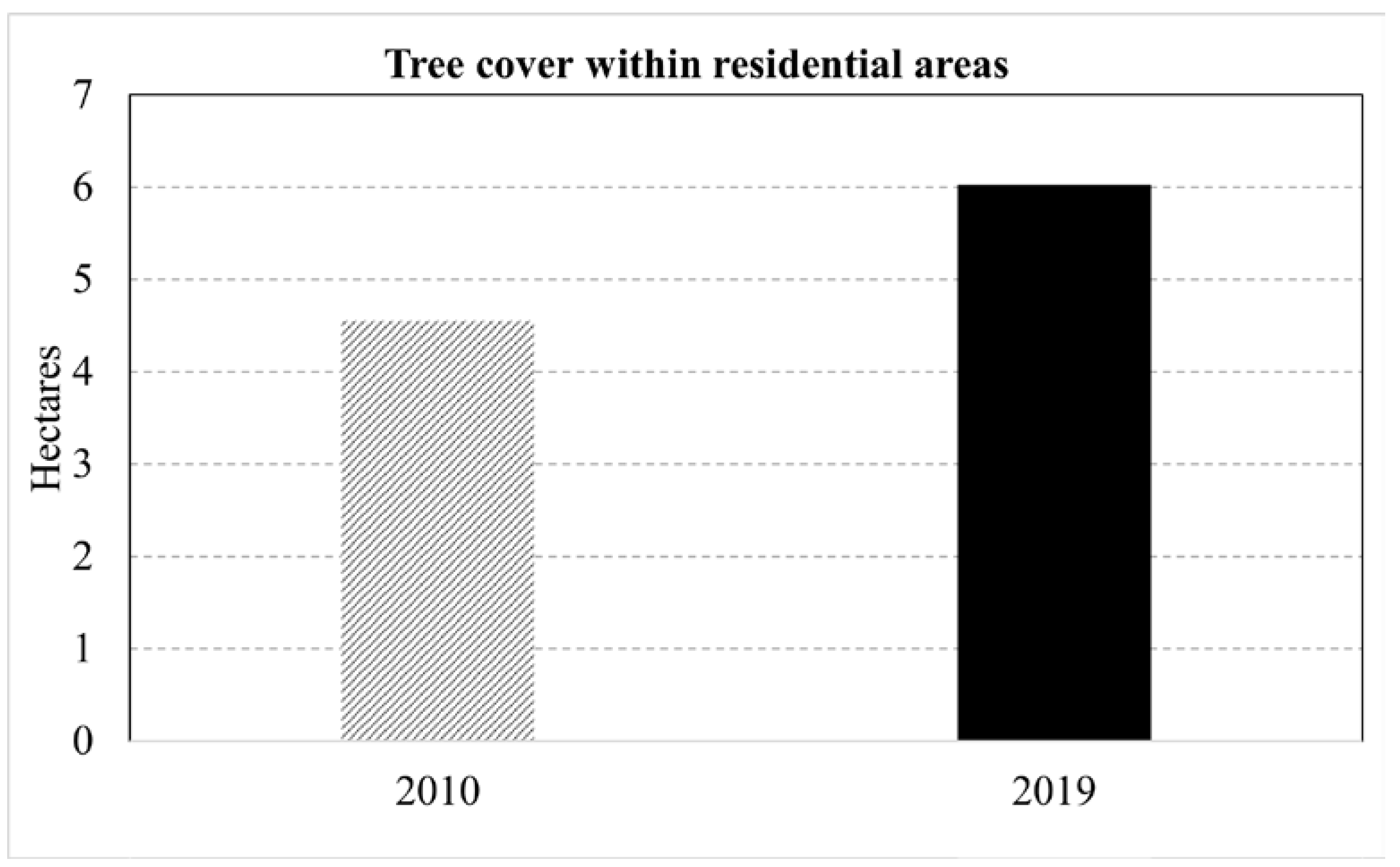
This paper demonstrated that FCNN models that utilize texture information in a fully automated, end-to-end mapping outperformed pixel-based conventional machine learning approaches in mapping tropical rainforest habitats. Our results showed that the FCNN model (U-Net) produced an overall accuracy of 90.9% compared to accuracies of 88.6%, 84.8%, and 86.6% for SVM, RF, and DNN models respectively. Moreover, the WV-3 SWIR bands increased the accuracy by 1.87% for the U-Net model. The decrease in accuracy without SWIR bands was much greater for DNN (8.55%), SVM (5.42%) and RF (3.18%) models that use only spectral features for classification, demonstrating the potential of the FCNN approach without using expansive SWIR data collections. Comparing LCLU maps generated in 2010 and 2019, changes in classes were quantified to understand human interactions with the environment and quantify the impact of conservation efforts. A 44% increase in Residential is seen in the study area, and a decrease in Row Crops in the ZOP. Within the BNR, invasive plant species are seen to decrease, which is complemented by increases in Mixed (12%) and Evergreen Forest (0.7%). This increase in forest cover indicates a reversal of the trends described by Ghulam et al. (2014). In addition, a 32% increase is seen in the tree cover within residential areas either due to native tree maturing or successful agroforestry efforts by the MFG. Conservation efforts worldwide should consider the needs of the local human population. As such, future conservation efforts by the MFG include improving human health and recognizing the importance of people-oriented strategies in order to provide cash crops and a sustainable food source for the locals.
Machine/deep learning has been far advanced in some application domains; however, challenges exist for remote sensing applications especially for tropical forest monitoring due to in part the lack of sufficient training data representing various biomes and forest types globally that must be manually created and in part the challenges of managing and analyzing big satellite data at the global scale. We presented a fully automated deep learning model in this paper which can be applied to any part of the world. Taking advantage of cloud computing, the approach can be duplicated for national-scale forest cover mapping and change detection, which has significant impact on our understanding of tropical forests and biodiversity for better implementation of REDD+.

Author Contributions

Conceptualization, V.S. and K.F.; methodology, V.S. and M.M.; software, G.C.; validation, G.C., V.S. and K.F.; formal analysis, G.C.; investigation, V.S.; resources, V.S. and K.F.; data curation, V.S.; writing—original draft preparation, G.C.; writing—review and editing, V.S. and K.F.; visualization, G.C. and V.S.; supervision, V.S.; project administration, V.S.; funding acquisition, V.S. and K.F. All authors have read and agreed to the published version of the manuscript.

Funding

The funding for this project is provided by Saint Louis University Geospatial Institute (GeoSLU), NASA #80NSSC20M0100, and IUCN’s SOS Lemurs grant #2017A-093.

Data Availability Statement

WorldView-3 imagery can be obtained from MAXAR technologies directly. Ground truth data and codes will be made available at https://github.com/remotesensinglab.

Acknowledgments

The ground reference data were collected thanks to Madagascar Flora and Fauna Group’s in situ data collection team. A minimal cloud-free image was acquired thanks to multiple satellite tasking by Digital Globe.

Conflicts of Interest

The authors declare no conflict of interest.

References

  1. FAO. REDD+ Reducing Emissions from Deforestation and Forest Degradation. Available online: http://www.fao.org/redd/en/ (accessed on 27 August 2021).
  2. UN. What Is REDD+? Available online: https://unfccc.int/topics/land-use/workstreams/redd/what-is-redd (accessed on 27 August 2021).
  3. Goodman, S.M.; Benstead, J.P. Updated estimates of biotic diversity and endemism for Madagascar. Oryx 2005, 39, 73–77. [Google Scholar] [CrossRef] [Green Version]
  4. Vieilledent, G.; Grinand, C.; Rakotomalala, F.A.; Ranaivosoa, R.; Rakotoarijaona, J.R.; Allnutt, T.F.; Achard, F. Combining global tree cover loss data with historical national forest cover maps to look at six decades of deforestation and forest fragmentation in Madagascar. Biol. Conserv. 2018, 222, 189–197. [Google Scholar] [CrossRef]
  5. Golden, C.D.; Rabehatonina, J.G.; Rakotosoa, A.; Moore, M. Socio-ecological analysis of natural resource use in Betampona Strict Natural Reserve. Madag. Conserv. Dev. 2014, 9, 83–89. [Google Scholar] [CrossRef]
  6. Armstrong, A.H.; Shugart, H.H.; Fatoyinbo, T.E. Characterization of community composition and forest structure in a Madagascar lowland rainforest. Trop. Conserv. Sci. 2011, 4, 428–444. [Google Scholar] [CrossRef] [Green Version]
  7. Gibson, L.; Lynam, A.J.; Bradshaw, C.J.A.; He, F.L.; Bickford, D.P.; Woodruff, D.S.; Bumrungsri, S.; Laurance, W.F. Near-Complete Extinction of Native Small Mammal Fauna 25 Years after Forest Fragmentation. Science 2013, 341, 1508–1510. [Google Scholar] [CrossRef] [PubMed]
  8. Rosa, G.M.; Andreone, F.; Crottini, A.; Hauswaldt, J.S.; Noel, J.; Rabibisoa, N.H.; Randriambahiniarime, M.O.; Rebelo, R.; Raxworthy, C.J. The amphibians of the relict Betampona low-elevation rainforest, eastern Madagascar: An application of the integrative taxonomy approach to biodiversity assessments. Biodivers. Conserv. 2012, 21, 1531–1559. [Google Scholar] [CrossRef]
  9. Kull, C.A.; Tassin, J.; Carrière, S.M. Approaching invasive species in Madagascar. Madag. Conserv. Dev. 2014, 9, 60–70. [Google Scholar] [CrossRef]
  10. Ghulam, A.; Porton, I.; Freeman, K. Detecting subcanopy invasive plant species in tropical rainforest by integrating optical and microwave (InSAR/PolInSAR) remote sensing data, and a decision tree algorithm. ISPRS J. Photogramm. 2014, 88, 174–192. [Google Scholar] [CrossRef]
  11. Ratovonamana, R.Y. Ecological Study of Exotic Invasive Plants in the RNI No 1 of Betampona in the Region of Toamasina, Madagascar; Department of Plant Ecology, University of Antananarivo: Antananarivo, Madagascar, 2006. [Google Scholar]
  12. Den Biggelaar, C.; Moore, M. The Changing Nature of Agricultural Livelihoods along a Peri-urban to Rural Gradient in Eastern Madagascar. Am. J. Rural Dev. 2016, 4, 31–42. [Google Scholar]
  13. Farris, A.R.; Misyak, S.; O’Keefe, K.; VanSicklin, L.; Porton, I. Understanding the drivers of food choice and barriers to diet diversity in Madagascar. J. Hunger Environ. Nutr. 2020, 15, 388–400. [Google Scholar] [CrossRef]
  14. Ghulam, A. Monitoring Tropical Forest Degradation in Betampona Nature Reserve, Madagascar Using Multisource Remote Sensing Data Fusion. IEEE J. Sel. Top. Appl. Earth Obs. Remote Sens. 2014, 7, 4960–4971. [Google Scholar] [CrossRef]
  15. Pandey, P.C.; Koutsias, N.; Petropoulos, G.P.; Srivastava, P.K.; Ben Dor, E. Land use/land cover in view of earth observation: Data sources, input dimensions, and classifiers—A review of the state of the art. Geocarto Int. 2019, 36, 957–988. [Google Scholar] [CrossRef]
  16. Lee, S.-H.; Han, K.-J.; Lee, K.; Lee, K.-J.; Oh, K.-Y.; Lee, M.-J. Classification of Landscape Affected by Deforestation Using High-Resolution Remote Sensing Data and Deep-Learning Techniques. Remote Sens. 2020, 12, 3372. [Google Scholar] [CrossRef]
  17. Wagner, F.H.; Sanchez, A.; Tarabalka, Y.; Lotte, R.G.; Ferreira, M.P.; Aidar, M.P.; Gloor, E.; Phillips, O.L.; Aragao, L.E. Using the U-net convolutional network to map forest types and disturbance in the Atlantic rainforest with very high resolution images. Remote Sens. Ecol. Conserv. 2019, 5, 360–375. [Google Scholar] [CrossRef] [Green Version]
  18. Ferreira, M.P.; Wagner, F.H.; Aragao, L.E.O.C.; Shimabukuro, Y.E.; de Souza, C.R. Tree species classification in tropical forests using visible to shortwave infrared WorldView-3 images and texture analysis. ISPRS J. Photogramm. 2019, 149, 119–131. [Google Scholar] [CrossRef]
  19. Hartling, S.; Sagan, V.; Sidike, P.; Maimaitijiang, M.; Carron, J. Urban Tree Species Classification Using a WorldView-2/3 and LiDAR Data Fusion Approach and Deep Learning. Sensors 2019, 19, 1284. [Google Scholar] [CrossRef] [PubMed] [Green Version]
  20. LeCun, Y.; Bengio, Y.; Hinton, G. Deep learning. Nature 2015, 521, 436–444. [Google Scholar] [CrossRef] [PubMed]
  21. Kussul, N.; Lavreniuk, M.; Skakun, S.; Shelestov, A. Deep Learning Classification of Land Cover and Crop Types Using Remote Sensing Data. IEEE Geosci. Remote Sens. Lett. 2017, 14, 778–782. [Google Scholar] [CrossRef]
  22. Krizhevsky, A.; Sutskever, I.; Hinton, G.E. Imagenet classification with deep convolutional neural networks. Adv. Neural. Inf. Process. Syst. 2012, 25, 1097–1105. [Google Scholar] [CrossRef]
  23. Simonyan, K.; Zisserman, A. Very deep convolutional networks for large-scale image recognition. arXiv 2014, arXiv:1409.1556. preprint. [Google Scholar]
  24. He, K.; Zhang, X.; Ren, S.; Sun, J. Deep residual learning for image recognition. In Proceedings of the IEEE Conference on Computer Vision and Pattern Recognition, Las Vegas, NV, USA, 27–30 June 2016; pp. 770–778. [Google Scholar]
  25. Huang, G.; Liu, Z.; Van Der Maaten, L.; Weinberger, K.Q. Densely connected convolutional networks. In Proceedings of the IEEE Conference on Computer Vision and Pattern Recognition, Honolulu, HI, USA, 21–26 July 2017; pp. 4700–4708. [Google Scholar]
  26. Long, J.; Shelhamer, E.; Darrell, T. Fully convolutional Networks for semantic segmentation. In Proceedings of the IEEE Conference on Computer Vision and Pattern Recognition, Boston, MA, USA, 7–12 June 2015; pp. 3431–3440. [Google Scholar]
  27. Ronneberger, O.; Fischer, P.; Brox, T. U-net: Convolutional networks for biomedical image segmentation. In Proceedings of the International Conference on Medical Image Computing and Computer-Assisted Intervention, Strabourg, France, 27 September–1 October 2021; pp. 234–241. [Google Scholar]
  28. Badrinarayanan, V.; Kendall, A.; Cipolla, R. Segnet: A deep convolutional encoder-decoder architecture for image segmentation. IEEE Trans. Pattern Anal. Mach. Intell. 2017, 39, 2481–2495. [Google Scholar] [CrossRef] [PubMed]
  29. Fu, G.; Liu, C.; Zhou, R.; Sun, T.; Zhang, Q. Classification for high resolution remote sensing imagery using a fully convolutional network. Remote Sens. 2017, 9, 498. [Google Scholar] [CrossRef] [Green Version]
  30. Han, Z.M.; Dian, Y.Y.; Xia, H.; Zhou, J.J.; Jian, Y.F.; Yao, C.H.; Wang, X.; Li, Y. Comparing Fully Deep Convolutional Neural Networks for Land Cover Classification with High-Spatial-Resolution Gaofen-2 Images. ISPRS Int. J. Geo-Inf. 2020, 9, 478. [Google Scholar] [CrossRef]
  31. Ji, S.; Wang, D.; Luo, M. Generative adversarial network-based full-space domain adaptation for land cover classification from multiple-source remote sensing images. IEEE Trans. Geosci. Remote 2020, 59, 3816–3828. [Google Scholar] [CrossRef]
  32. Zhu, Y.; Geiss, C.; So, E.M.; Jin, Y. Multitemporal Relearning with Convolutional LSTM Models for Land Use Classification. IEEE J. Sel. Top. Appl. Earth Obs. Remote Sens. 2021, 14, 3251–3265. [Google Scholar] [CrossRef]
  33. Yuan, Q.Q.; Shen, H.F.; Li, T.W.; Li, Z.W.; Li, S.W.; Jiang, Y.; Xu, H.Z.; Tan, W.W.; Yang, Q.Q.; Wang, J.W.; et al. Deep learning in environmental remote sensing: Achievements and challenges. Remote Sens. Environ. 2020, 241, 11176. [Google Scholar] [CrossRef]
  34. Hamdi, Z.M.; Brandmeier, M.; Straub, C. Forest Damage Assessment Using Deep Learning on High Resolution Remote Sensing Data. Remote Sens. 2019, 11, 1976. [Google Scholar] [CrossRef] [Green Version]
  35. Pacifici, F.; Longbotham, N.; Emery, W.J. The Importance of Physical Quantities for the Analysis of Multitemporal and Multiangular Optical Very High Spatial Resolution Images. IEEE Trans. Geosci. Remote 2014, 52, 6241–6256. [Google Scholar] [CrossRef]
  36. Smith, M.J. A Comparison of DG AComp, FLAASH and QUAC Atmospheric Compensation Algorithms Using WorldView-2 Imagery. Available online: https://digitalglobe-marketing.s3.amazonaws.com/files/blog/MichaelSmith_Masters_Report_ACOMP_Assessment.pdf (accessed on 1 August 2020).
  37. Kuester, M. Radiometric Use of Worldview-3 Imagery; DigitalGlobe: Longmont, CO, USA, 2016. [Google Scholar]
  38. DigitalGlobe. Geolocation Accuracy of WorldView Products. Available online: https://rmgsc.cr.usgs.gov/outgoing/KramerLBNL/WorldView_Geolocation_Accuracy.pdf (accessed on 12 August 2021).
  39. ArcGIS API for Python. Available online: https://developers.arcgis.com/python/ (accessed on 27 August 2021).
  40. Giang, T.L.; Dang, K.B.; Le, Q.T.; Nguyen, V.G.; Tong, S.S.; Pham, V. U-Net Convolutional Networks for Mining Land Cover Classification Based on High-Resolution UAV Imagery. IEEE Access 2020, 8, 186257–186273. [Google Scholar] [CrossRef]
  41. Cortes, C.; Vapnik, V. Support-Vector Networks. Mach. Learn. 1995, 20, 273–297. [Google Scholar] [CrossRef]
  42. Fauvel, M.; Chanussot, J.; Benediktsson, J.A. Evaluation of kernels for multiclass classification of hyperspectral remote sensing data. In Proceedings of the 2006 IEEE International Conference on Acoustics Speech and Signal Processing Proceedings, Toulouse, France, 14–19 May 2006; p. II. [Google Scholar]
  43. Breiman, L. Random forests. Mach. Learn. 2001, 45, 5–32. [Google Scholar] [CrossRef] [Green Version]
  44. Olofsson, P.; Foody, G.M.; Stehman, S.V.; Woodcock, C.E. Making better use of accuracy data in land change studies: Estimating accuracy and area and quantifying uncertainty using stratified estimation. Remote Sens. Environ. 2013, 129, 122–131. [Google Scholar] [CrossRef]
  45. Ghulam, A.; Ghulam, O.; Maimaitijiang, M.; Freeman, K.; Porton, I.; Maimaitiyiming, M. Remote Sensing Based Spatial Statistics to Document Tropical Rainforest Transition Pathways. Remote Sens. 2015, 7, 6257–6279. [Google Scholar] [CrossRef] [Green Version]
  46. Li, M.; Zang, S.Y.; Zhang, B.; Li, S.S.; Wu, C.S. A Review of Remote Sensing Image Classification Techniques: The Role of Spatio-contextual Information. Eur. J. Remote Sens. 2014, 47, 389–411. [Google Scholar] [CrossRef]
  47. Marmanis, D.; Datcu, M.; Esch, T.; Stilla, U. Deep Learning Earth Observation Classification Using ImageNet Pretrained Networks. IEEE Geosci. Remote Sens. Lett. 2016, 13, 105–109. [Google Scholar] [CrossRef] [Green Version]
  48. Tsai, Y.H.; Stow, D.; Chen, H.L.; Lewison, R.; An, L.; Shi, L. Mapping Vegetation and Land Use Types in Fanjingshan National Nature Reserve Using Google Earth Engine. Remote Sens. 2018, 10, 927. [Google Scholar] [CrossRef] [Green Version]
  49. Sidike, P.; Sagan, V.; Maimaitijiang, M.; Maimaitiyiming, M.; Shakoor, N.; Burken, J.; Mockler, T.; Fritschi, F.B. dPEN: Deep Progressively Expanded Network for mapping heterogeneous agricultural landscape using WorldView-3 satellite imagery. Remote Sens. Environ. 2019, 221, 756–772. [Google Scholar] [CrossRef]
  50. Jensen, J.R. Introductory Digital Image Processing: A Remote Sensing Perspective, 3rd ed.; Prentice-Hall: Upper Saddle River, NJ, USA, 2005. [Google Scholar]
  51. DeFries, R.; Karanth, K.K.; Pareeth, S. Interactions between protected areas and their surroundings in human-dominated tropical landscapes. Biol. Conserv. 2010, 143, 2870–2880. [Google Scholar] [CrossRef]
  52. Styger, E.; Rakotondramasy, H.M.; Pfeffer, M.J.; Fernandes, E.C.M.; Bates, D.M. Influence of slash-and-burn farming practices on fallow succession and land degradation in the rainforest region of Madagascar. Agric. Ecosyst. Environ. 2007, 119, 257–269. [Google Scholar] [CrossRef]
Figure 1. (a) WorldView-3 0.3 m pansharpened RGB imagery with minimal cloud cover, over the study area—the Betampona Nature Reserve (BNR) (white boundary polygon), located on the (b) eastern coast of Madagascar, which is (c) an island to the southeast of Africa.
Remotesensing 13 03495 g001
Figure 2. In situ images of a few classes being mapped, collected during the ground reference data collection in 2018. Additional classes include invasive guava, residential, and open water.
Remotesensing 13 03495 g002
Figure 3. U-net architecture with the encoding (left) and decoding (right) sections that produce the characteristic U-shape of the architecture, producing pixel-wise classification of the input imagery. ResNet layers forms the encoder.
Remotesensing 13 03495 g003
Figure 4. Network architecture implemented for the Deep Neural Network (DNN) model along with the number of neurons that were optimized for each hidden layer. The output layer contains 11 neurons, corresponding to the number of classes to be classified.
Remotesensing 13 03495 g004
Figure 5. F1 score (Equation (6)), for all classes and models, showing the superiority of the FCNN U-Net model.
Remotesensing 13 03495 g005
Figure 6. Comparison of confusion matrixes for (a) DNN where SWIR bands were included, (b) DNN where SWIR bands were excluded, (c) U-Net where SWIR bands were included, and (d) U-Net where SWIR bands were excluded. A greater number of FPs and FNs are seen in (b,d) because of the removal of the SWIR bands. The DNN and U-Net models are chosen for comparison because of the highest and lowest reduction in accuracy due to the removal of SWIR.
Remotesensing 13 03495 g006
Figure 7. F1 scores (Equation (6)) for the U-Net and DNN models including (16 bands) and excluding (8 bands) SWIR bands across all classes. The U-Net and DNN models trained on 16 bands show a higher F1 score compared to the models trained on eight bands.
Remotesensing 13 03495 g007
Figure 8. Detailed and highly accurate classification map of the BNR and surrounding areas, created using WorldView-3 imagery and post-classification editing, showing the distribution of 11 classes.
Remotesensing 13 03495 g008
Figure 9. (a) The 2010 classification map and (b) the associated classification map created in 2019. The use of identical classes enabled the quantification of land cover change over time.
Remotesensing 13 03495 g009
Figure 10. Residential areas in 2019 (red boundary polygon) in the study area (extent shown in inset map) overlain over the 2010 classification map showing the increase in residential area extent and the emergence of new hamlets in 2019 for (a) a location east of the BNR and (b) northwest of the BNR.
Remotesensing 13 03495 g010
Figure 11. An increase in tree cover in residential areas in hectares from 2010 (gray diagonal bar) to 2019 (black solid bar) is attributed to maturing native trees and successful agroforestry efforts.
Remotesensing 13 03495 g011
Figure 12. Percentage of classes in 2010 that were converted to Shrubland in 2019, within the study area based on the classification map extent seen in Figure 9. This information is useful for awareness-raising and conservation efforts.
Remotesensing 13 03495 g012
Figure 13. Evergreen Forest areas in 2010 (green boundary polygons) that were converted to Shrubland in 2019 located east of the BNR, overlaid over the 2019 classification map. The inset map shows the 2019 classification map.
Remotesensing 13 03495 g013
Figure 14. Percentage of classes in 2010 that were converted to Mixed Forest in 2019 within the BNR, shows a higher conversion of invasive plants—Molucca Raspberry, Madagascar Cardamom, and Guava—to Mixed Forest compared to Evergreen Forest.
Remotesensing 13 03495 g014
Figure 15. Invasive plant species within the BNR and the land cover types seen 100 m within the BNR boundary (gray line) and within the ZOP (100 m extending from the BNR boundary). Forest covers are observed along with a few scattered agricultural fields within the 200 m wide region on two sides of the boundary. Note that wider streams represented by the Open Water class are located further south of this map extent, which is not visible here. The Open Water and Streams classes should be treated as the same class.
Remotesensing 13 03495 g015
Figure 16. Classification map created using the SVM model, with an 88.6% overall accuracy, zoomed into a location on the western section of the BNR that shows the salt-and-pepper effect.
Remotesensing 13 03495 g016
Figure 17. Reflectance spectra of all classes, showing the overlapping reflectance spectra for vegetation classes—for example between Evergreen Forest, Grassland, and Mixed Forest.
Remotesensing 13 03495 g017
Figure 18. F1 scores of all classification methods employed including (16 bands) and excluding SWIR bands (8 bands), showing the percent change due to the removal of SWIR bands for (a) Guava, (b) Madagascar Cardamom, (c) Evergreen Forest, (d) Mixed Forest, (e) Molucca Raspberry, (f) Row Crops, (g) Residential, (h) Fallow, (i) Shrubland, and (j) Grassland.
Remotesensing 13 03495 g018
Figure 19. Percent change of (a) Evergreen Forest and (b) Agriculture—including Row Crops and Fallow—over the BNR overlain over a DEM, showing areas of increased (red) and decreased (blue) extents based on a 10 m × 10 m grid cell. The BNR boundary is shown via the black line and the ZOP and 100 m region within the BNR used for change analysis is displayed through the gray polygon.
Remotesensing 13 03495 g019
Table 1. This table lists the classes and descriptions used in order to create the classification map. Eleven classes were defined that relate to land cover (Open Water, Row Crops), land use (Residential, Fallow), and forest cover (Mixed Forest, Evergreen Forest, Molucca Raspberry, Shrubland, Madagascar Cardamom, Grassland and Guava).
ClassesDescription
Mixed ForestYoung and mixed forest or degraded forest
Evergreen ForestPristine and degraded forest
ResidentialBuilt-up areas
Molucca RaspberryInvasive plant species
Row cropsAgricultural land
FallowArea cleared prior to planting
ShrublandShrubs dominating the land cover
Open WaterWater bodies within the study area, i.e., rivers, streams
Madagascar CardamomPlant species invasive to Betampona region
GrasslandGrasses dominating the land cover
GuavaInvasive plant species
Table 2. Results—overall accuracy (Equation (2)), kappa coefficient (Equation (3)), producer’s (Equation (4)), and user’s accuracy (Equation (5)) for Support Vector Machine (SVM), Random Forest (RF), Deep Neural Network (DNN), and U-Net models, based on independent testing data.
Accuracy MetricClassification ClassU-NetSVMRFDNN
Producer’s Accuracy Mixed Forest91.567.564.570.2
Evergreen Forest78.669.959.468.8
Residential100.097.898.488.2
Molucca Raspberry95.496.799.499.4
Row Crops96.997.690.392.8
Fallow100.095.491.099.0
Shrubland79.879.276.272.0
Open water100.0100.0100.0100.0
Madagascar Cardamom81.690.080.093.3
Grassland81.688.785.081.7
Guava89.882.080.681.0
User’s AccuracyMixed Forest82.275.870.672.3
Evergreen Forest85.175.164.168.2
Residential99.995.189.899.0
Molucca Raspberry95.596.096.399.8
Row Crops100.098.995.494.2
Fallow100.098.298.791.0
Shrubland70.875.067.780.7
Open Water100.0100.0100.0100.0
Madagascar Cardamom84.581.877.576.9
Grassland97.393.993.793.2
Guava81.372.971.273.4
Overall Accuracy (%) 90.988.684.886.6
Kappa Coefficient 0.9010.8750.8350.854
Table 3. Overall accuracy (Equation (2)) and percent change for all classification models including (16 bands) and excluding (8 bands) the shortwave infrared (SWIR) bands.
Accuracy MetricU-NetSVMRFDNN
Overall Accuracy (%) (16 bands)90.988.684.886.6
Overall Accuracy (%) (8 bands)89.283.882.179.2
Percent Decrease −1.87−5.42−3.18−8.55
Table 4. Percentage and area in hectares of each class type mapped in 2019 within the study area, based on the classification map seen in Figure 8.
Classes2019 (%)2019 (ha)
Mixed Forest19.7432,990.21
Evergreen Forest13.2222,099.87
Residential 0.38650.62
Molucca Raspberry1.312190.60
Row Crops3.085147.37
Fallow4.978313.04
Shrubland48.5581,148.99
Open Water1.392327.05
Madagascar Cardamom2.023386.98
Grassland3.816369.07
Guava1.492490.60
Table 5. Total hectares for each class mapped in 2010 and 2019 are listed below based on overlapping extent (Figure 9), along with the amount of percent increase (or decrease) (Equation (7)) over time for each class.
Classification Category2010 (%)2019 (%)Percent Change
Mixed Forest18.1519.044.87
Evergreen Forest21.5221.851.54
Residential 0.230.3344.31
Molucca Raspberry3.271.45−55.69
Row Crops6.432.82−56.13
Fallow6.034.16−31.01
Shrubland31.1142.6937.22
Open Water0.620.9553.57
Madagascar Cardamom0.861.2647.49
Grassland9.803.59−63.39
Guava1.981.86−6.10
Table 6. Percentage of forest cover types in 2010 and 2019 observed within the boundary of the BNR (Figure 1).
Forest Cover Class2010 (%)2019 (%)Percent Change
Mixed Forest10.311.512.5
Evergreen Forest81.081.60.7
Molucca Raspberry1.81.3−28.4
Madagascar Cardamom2.52.2−12.8
Guava3.13.1−0.3
Table 7. Percentage of classes within the ZOP, a 100 m buffer zone that borders the BNR. Invasive forest cover types are highlighted.
Classes2010 (%)2019 (%)Percent Change (%)
Mixed Forest16.5521.2328.36
Evergreen Forest16.8226.7959.43
Residential 0.150.12−17.91
Molucca Raspberry8.422.70−67.93
Row Crops11.272.69−76.13
Fallow1.511.43−4.93
Shrubland25.6330.2318.04
Open water0.070.36430.64
Madagascar Cardamom5.265.260.06
Grassland10.031.99−80.13
Guava4.297.2168.09
Table 8. Accuracy metrics—overall accuracy (Equation (2)) and kappa coeff. (Equation (3))—based on the predictions of best performing models, SVM and U-Net, compared with the edited map seen in Figure 8. The accuracy of modelsis much lower compared to the accuracy derived from independent testing data.
Model NameAccuracy (%) Kappa Coeff.
SVM66.50.650
U-Net77.30.655
Publisher’s Note: MDPI stays neutral with regard to jurisdictional claims in published maps and institutional affiliations.

