
Reliable Estimates of Merchantable Timber Volume from Terrestrial Laser Scanning


Faculty of Forestry and Wood Sciences, Czech University of Life Sciences (CZU Prague), Kamýcká 129, 165 21 Prague, Czech Republic
*
Author to whom correspondence should be addressed.
Remote Sens. 2021, 13(18), 3610; https://0-doi-org.brum.beds.ac.uk/10.3390/rs13183610
Submission received: 28 July 2021
/
Revised: 19 August 2021
/
Accepted: 8 September 2021
/
Published: 10 September 2021
(This article belongs to the Special Issue Terrestrial Laser Scanning of Forest Structure)
Abstract
:Simple and accurate determination of merchantable tree height is needed for accurate estimations of merchantable volume. Conventional field methods of forest inventory can lead to biased estimates of tree height and diameter, especially in complex forest structures. Terrestrial laser scanner (TLS) data can be used to determine merchantable height and diameter at different heights with high accuracy and detail. This study focuses on the use of the random sampling consensus method (RANSAC) for generating the length and diameter of logs to estimate merchantable volume at the tree level using Huber’s formula. For this study, we used two plots; plot A contained deciduous trees and plot B consisted of conifers. Our results demonstrated that the TLS-based outputs for stem modelling using the RANSAC method performed very well with low bias (0.02 for deciduous and 0.01 for conifers) and a high degree of accuracy (97.73% for deciduous and 96.14% for conifers). We also found a high correlation between the proposed method and log length (−0.814 for plot A and −0.698 for plot B), which is an important finding because this information can be used to determine the optimum log properties required for analyzing stem curvature changes at different heights. Furthermore, the results of this study provide insight into the applicability and ergonomics during data collection from forest inventories solely from terrestrial laser scanning, thus reducing the need for field reference data.
1. Introduction
Overpopulation has placed increased pressure on forest resources worldwide, and the demands for developing accurate and efficient forecasting and planning has also increased. Forest inventories are the main tool used to describe forest structure and quantify forest resources [1]. Precise estimation of volume is an essential factor in a forest management plan (FMP). Volume estimation provides the volume of wood in the forest and directly or indirectly can be used to determine forest biomass, the amount of carbon storage and sequestration (with increasing concern of climate change issues), and the fuel source. Current information on merchantable timber volume is a key element in sustainable forest management, for wood products and their potential value at market prices [2]. Until recently, forests were mainly inventoried manually using conventional approaches, which often resulted in biased estimations. Merchantable volume is a function of two important tree variables: (a) diameter and (b) height [3,4]. Diameter is commonly measured using calipers, logging tapes [5], and relascopes [6] in higher portions of the stem, while tree height or length is commonly measured using clinometers, laser rangefinders, hypsometers based on ultrasonic technology, and logging tapes [7,8]. Increasingly there is a need for regular and reliable updates of forest inventories (e.g., timber assessment of annual growth rates and stocking percentages) for planning and marketing purposes. Taper functions are widely used to estimate merchantable volume, as well as total trunk volume [9], and a variety of equations describing growth patterns for particular tree species have been used for the development of taper functions [10,11,12]. However, the applicability of well-calibrated taper functions is limited to only a few commercial tree species. Moreover, conventional methods for the construction of taper functions are usually laborious and costly. Aside from requiring felled trees to measure trunk diameter at different heights, sampling requires tree removal that can not only cause dynamic changes in forest structure, but its functionality may be altered as well [2,13,14].
Modern remote sensing technologies, such as light detection and ranging (LiDAR), offer the advantage of conducting inventory surveys automatically, with high quality and reliability. The applications of terrestrial laser scanning (TLS) have largely focused on modelling forest structural metrics, such as height [15,16,17,18], diameter [15,16,17,18], stem volume [8,19,20], above-ground biomass [21,22], and branch architecture [23], among others. These modern techniques have proven to be superior to conventional field surveys for a series of reasons. For example, precise identification of the correct upper stem height and diameters along different portions of the stem from detailed point clouds.
Terrestrial laser scanning also offers greater detail in terms of a spatial analysis, which results in less bias and higher accuracy compared with conventional field survey tools such as hypsometers, clinometers, rangefinders, and relascopes. Dassot et al. [18] proposed a semi-automatic method for modelling the merchantable stem volume of standing trees based on simple geometric fitting from TLS data. Comparisons with the field measurements demonstrated strong agreement between the datasets regardless of the tree species and size. More specifically, the relative differences of the TLS estimates remained primarily within a range of ±10% for estimating the merchantable stem volume. Similarly, Fernández-Sarría et al. [24] statistically explored the residual biomass after the extraction of the merchantable volume. According to their results, the highest accuracy was found when the voxel method was used for a pruned biomass volume prediction with R2 = 0.73. A study conducted by Yrttimaa et al. [25] demonstrated the feasibility of TLS in mapping forest biodiversity indicators; they introduced a method for quantifying downed dead wood using the random sampling consensus method (RANSAC) cylinder fitting approach and visual interpretation to aid in trunk detection. Their results showed that downed dead wood volume was automatically estimated with an RMSE of 15.0 m3/ha (59.3%), which was reduced to 6.4 m3/ha (25.3%) when visual interpretation was incorporated. In another study, Amiri et al. [26] used visual interpretation to identify all the reference stems, and they compared them with stems obtained through laser scanning. The evaluation of the automatically detected stems showed a classification precision of 0.86 and 0.85 and recall values of 0.7 and 0.67 for plots 1 and 2, respectively. Finally, Olofsson et al. [27] used a modified version of RANSAC and the Hough transform on TLS data to develop and validate a method for detecting and measuring stem attributes with high accuracy. Their results showed that the most accurate diameter measurements for pines were obtained with an RMSE of 7% for a defined plot radius of 20 m.
Although the algorithms have been researched to improve the TLS point cloud precision and accuracy [27,28,29], some algorithms and methods need further improvements, such as extracting forest attributes from TLS data and data acquisition protocols. These drawbacks that cannot be eliminated limit the processing efficiency and accuracy of extracting forest attributes [30].
To our knowledge, ours is the first attempt to utilize very dense TLS-based point clouds together with the RANSAC cylinder fitting method to extract the merchantable volumes of two widespread commercial tree species, European oak (Quercus robur L.) and Norway spruce (Picea abies (L.) H. Karst.). The objectives of this study were to (i) illustrate how TLS data can solely provide robust and reliable estimates of forest resources using the RANSAC method to accurately model merchantable stem volumes using two different experimental plots, and (ii) define the optimum log properties required for analyzing tree curvature changes at different heights to fully automate the process of log geometric fitting for merchantable height estimates.
2. Materials and Methods
2.1. Characterization of the Study Area
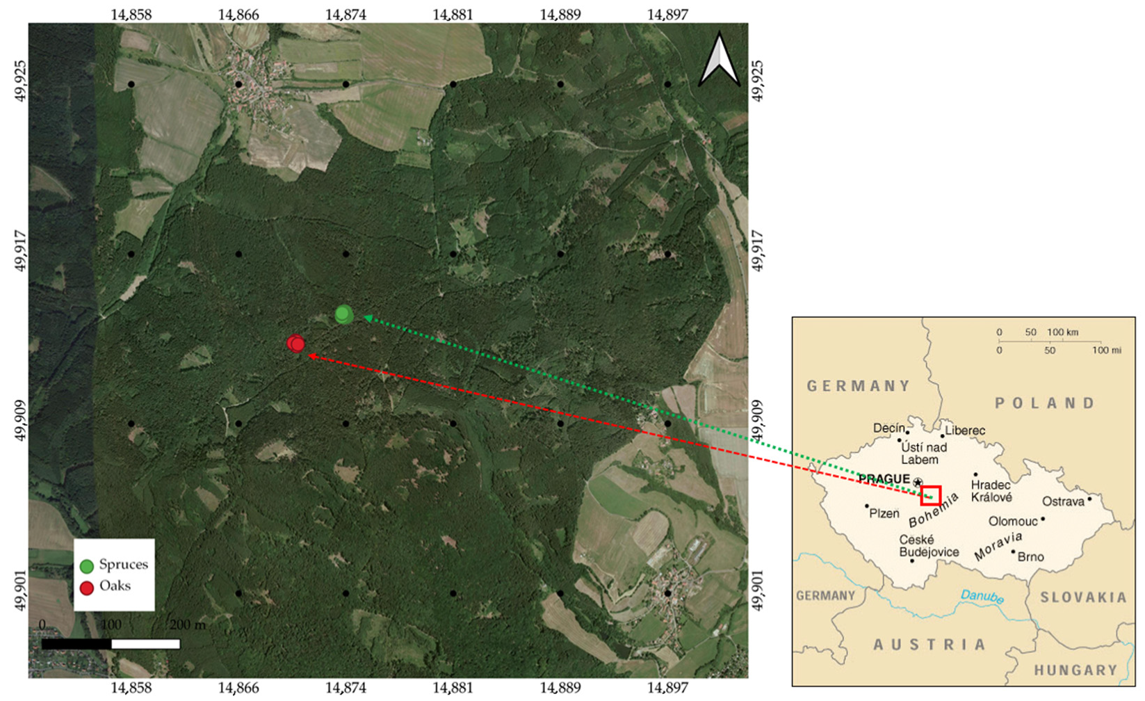
The research area is located in the School Forest Enterprise in Kostelec nad Černými lesy (Figure 1). We established two experimental plots, each 25 × 25 m in size; plot A (49°54′45.15″ N; 14°52′11.44″ E to 49°54′44.98″ N; 14°52′12.75″ E) is dominated by European oak, and plot B (49°54′50.19″ N; 14°52′23.61″ E to 49°54′50.12″ N; 14°52′24.98″ E) is comprised of Norway spruce. The terrain profile is gently sloping (0–5%), with an altitude of about 420 m a.s.l., a mean annual temperature of 7.5 °C, and mean annual precipitation of 600 mm. The area is mainly characterized by even-aged managed forests over the past 50-60 years.
2.2. TLS Data Acquisition and Pre-Processing
We used the Trimble TX8 scanning system (Trimble Inc. Sunnyvale, California USA, 1978); laser scanning was conducted on 26 August 2019. To ensure the optimal degree of overlap between the scanning positions, we used a multi-scan approach with a total of seven scans. The first scan was placed at the center of each plot and the rest were distributed along the periphery of each plot; the duration for each scan was 10 min. In addition to the scanning parameters, fixed exposure was disabled, and the third level of the scan density setting was used. The device provides a 360° × 317° field-of-view acquisition, enabling optimal scanning performance of high-resolution scans up to 120 m, and it generates 555 Mpts/per scan in third level mode. TLS has a maximum distance range of 120 m (for most surfaces), a scanning speed of 1 M pts/sec, and range systematic error of < 2 mm. To calibrate the laser scanner, the field instant method was used. To ensure better performance for the scan registration process, the laser scanner reference sphere set was used [31]. In parallel with the scans, marked wooden sticks were placed on the ground at each station. That permitted us to measure the scanning positions using the Trimble M3 total station, with an error of 2 mm in the horizontal distance. The registration of the point clouds was conducted in the RealWorks software (Trimble Inc. Sunnyvale, CA, USA, 1978) with a point density of 0.01 m for both plots.
2.3. Filtering of Ground and Off-Ground Points
After the pre-processing phase, the point clouds were extracted and imported in CloudCompare software V.2.10. (Zephyrus, Paris, France, 2011) [32], where the cloth simulation filter (CSF) algorithm [33] as a third-party plug-in was applied to separate and extract the ground from off-ground points. In the general parameter setting tab of the surface base filter, the relief terrain option was chosen due to the slightly inclined plane in both plots, whereas for calibration, cloth resolution was set to 1.1; as for maximum iterations, we used 500.
2.4. Sampling-Estimation and Measurement of Log Attributes
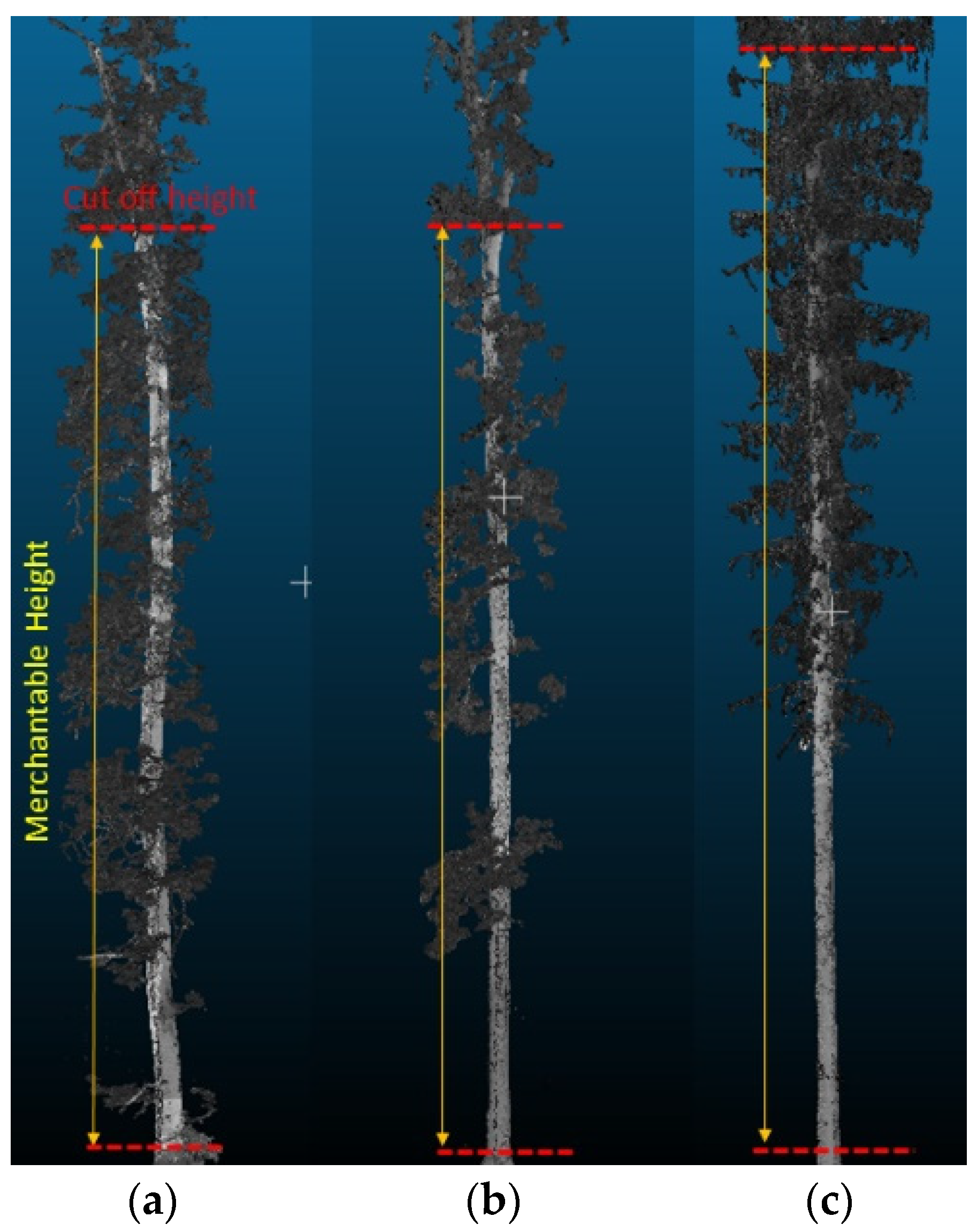
To derive the merchantable volume on each plot, 15 sample trees were randomly chosen. The merchantable height for both plots was determined by visual interpretation of the stem profile, from stump height until cut off height (Figure 2). For plot A, the oak site, the main bifurcation and the high degree of stem curvature were used as the main parameters for determining the cutting height (e.g., Figure 2a,b). If the tree did not have any of the above characteristics, the merchantable height for both deciduous and conifer trees was determined by measuring the smallest upper stem diameter (Figure 2c) (threshold ≥ 19 cm) [34] using the point picking tool in CloudCompare.
After the merchantable height for each tree was determined, the stems were segmented into several logs using the stem intercept method (point cloud segmentation).
The total number of logs (137 logs in plot A and 49 logs in plot B) was determined by visual interpretation (e.g., Figure 3). The higher the degree of stem curvature, the higher the number of logs produced. For the segmentation, the RANSAC algorithm [35] is adopted as a third-party plug-in in CloudCompare (Figure 4). RANSAC is an iterative process, to estimate parameters of a mathematical model from a set of observed data that contain outliers, outliers are to be accorded no influence on the values of the estimates [35]. Each iteration comprises of three primary steps.
The first step creates a minimal subset Pms of points, where Pms ⊂ Point Cloud = {p1, …, pN} and ms < N. This subset contains the minimum number of points needed to define a candidate shape (e.g., five for a cylinder). For the cylinder, one point is picked from the point cloud at a time, and a set of tests are performed to determine if the newly sampled point is on the same or a different shape face as the points already populating Pms. The newly sampled point is added if it lies on a different face respect to all points in Pms, otherwise it is discarded. The second step defines a candidate primitive shape from Pms. For cylinders the orientation of the shape is found using the normals to two of the points in Pms. Afterward, the size is determined from the whole set of points in Pms. Finally, the center is calculated from the reconstructed shape. The third step is to score the candidate’s primitive shape (Equation (1)) [36]:
where N is the number of points in the point cloud, δ(pi, I) is the shortest distance between pi and the surface of the candidate shape I, and ε is the error tolerance.
A cylinder is a good candidate for reaching the studied trees’ general shape to fit the produced logs (Figure 4). However, in the case of plot B, we did not consider a single fitted cylinder for modelling the entire merchantable height (from stump to cut off height). That is due to the differences in diameter at the upper and lower cross-section of each log. Therefore, to eliminate this bias each stem was also divided into logs (roughly 3). Although most of the trees in plot B were characterized by a high degree of stem straightness, stem curvature was also considered to determine the final number of logs produced.
In the general parameter settings tab of RANSAC shape recognition in CloudCompare, we used a cylinder as a primitive, (400 and 480 was the minimum support number of points per cylinder for plots A and B, while the maximum support number of points per cylinder was 880 and 770 for plots A and B, respectively). For the advanced parameters, based on the size and curvature of each stem, we used the maximum distance to the cylinder (parameter “e”) ranging from 0.004 to 0.084 for deciduous (plot A), and 0.005 to 0.077 for conifers (plot B), sampling resolution (parameter “b”), maximum normal deviation (parameter “a”), and overlook probability (default = 0.01). More details regarding the used parameters are described in Table S1.
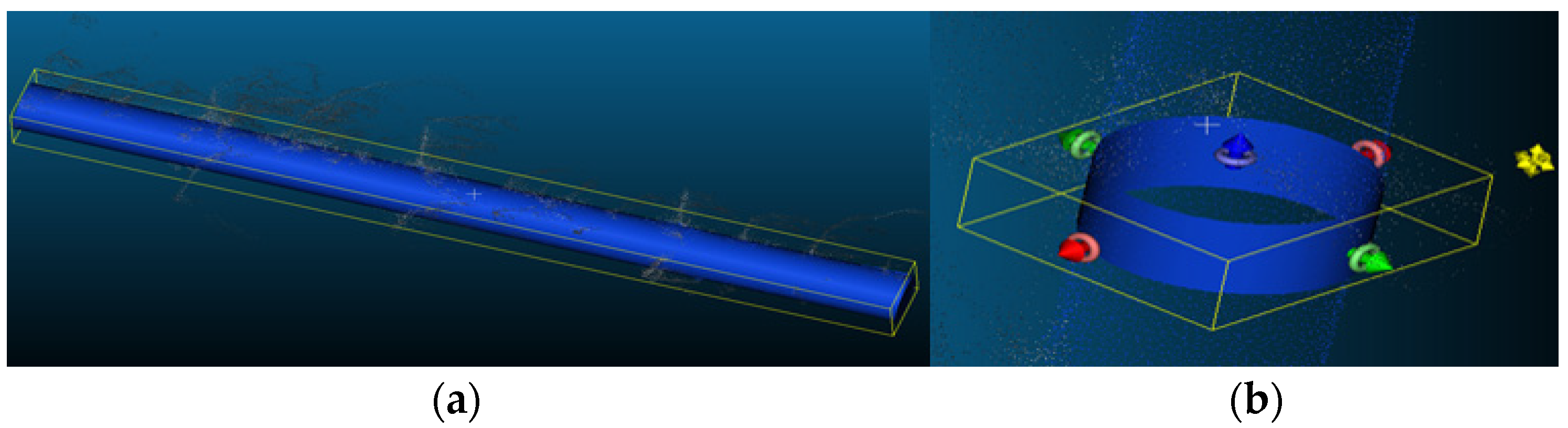
The results of the RANSAC adjustment for each log yielded the length (e.g., Figure 4a) and diameter in each cylinder (e.g., Figure 4b). Afterward, Huber’s formula (Equation (2)) was applied in each log to determine the estimated merchantable volume.
where π = 3.1416, D is the log diameter in the middle and L is the length of the log.
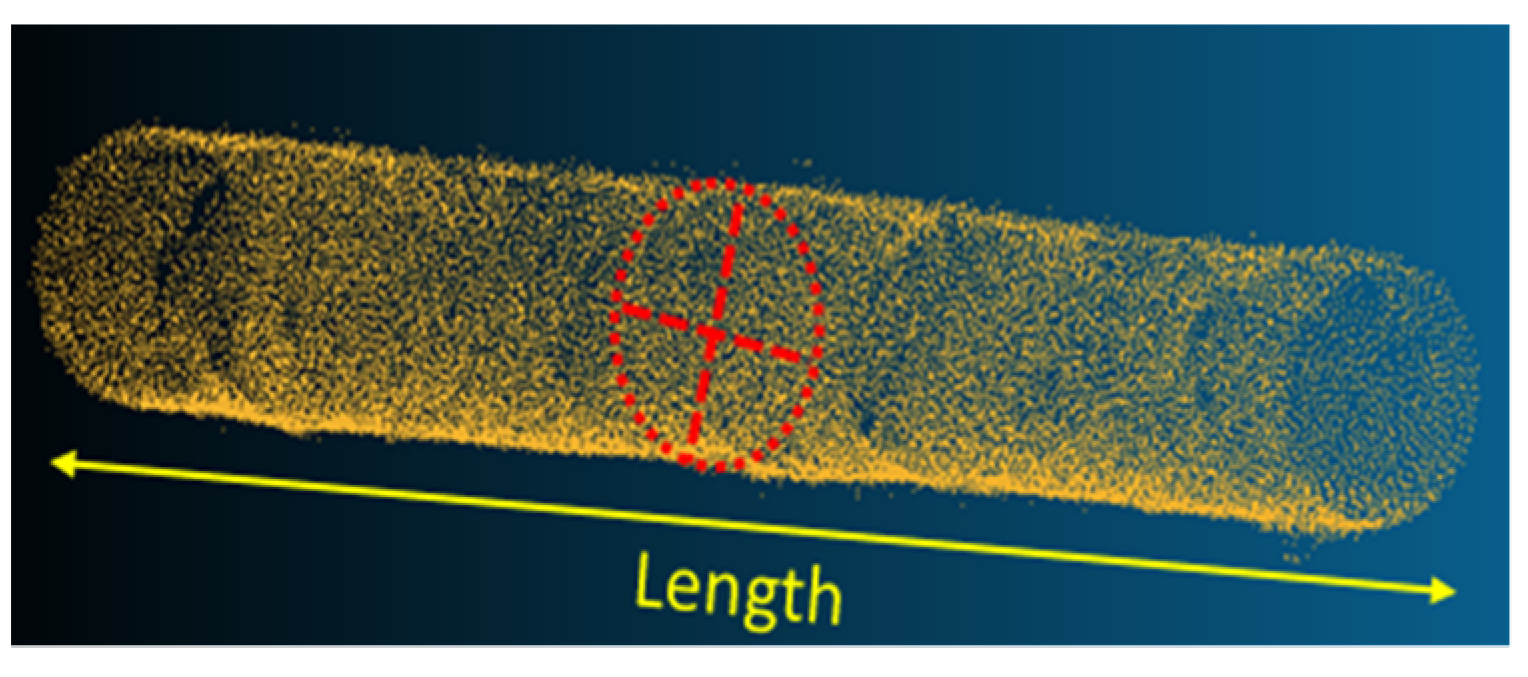
Concomitantly, we measured the length and the diameters of the extracted logs to be used as reference data. More specifically, the point picking tool was used to measure the length of each log (e.g., Figure 5). For log diameter, two diameters were measured from a perpendicular direction in the middle of each log using the same tool (e.g., Figure 5). Moreover, the point picking tool allowed us to locate the exact positions of the desired points with high precision. Simultaneously, we were able to rotate the log models in any direction, by holding any xyz axis without losing the reference plane, as well as the previous set selected. This allowed us to rotate the model 90 degrees and select two additional points, perpendicular to the initial points, thus preserving the methodological consistency. The final diameter was then determined as the average of these two measurements in each log.
2.5. Validation
We tested the normality of our data in both plots, and for plot A the measured and estimated data were normally distributed based on the Shapiro–Wilk and Kolmogorov–Smirnov tests. However, for plot B the measured and estimated data were not normally distributed based on Shapiro–Wilk and Kolmogorov–Smirnov tests.
For plot A we used a paired t-test, and for plot B the Wilcoxon signed-rank test was used. To investigate the relationship between calculated bias, volume residuals, and log attributes (diameter and length) we used the Spearman’s ρ correlation (Equation (3)). All statistical tests were considered significant at p-values less than 0.05.
where ρ is the Spearman’s rank correlation coefficient, is the difference between the two ranks of each observation, and n is the number of observations.
Linear regression was also used to model the relationship between the measured and estimated volumes. Accuracy assessment was performed at a tree-level to evaluate the accuracy of estimated merchantable volume by calculating the R-squared (Equation (4)), RMSE (Equation (5)), and RMSE% (Equation (6)).
where, and represent the estimated and measured values, respectively, refers to the average of the measured values, and n is the number of observations.
where is the estimated value, is the measured value, and n is the number of observations.
where is the root mean square error and is the average value.
Additionally, we used the following validation metrics; mean absolute deviation (MAD; Equation (7)), mean square error (MSE; Equation (8)), and mean absolute percentage error (MAPE; Equation (9)).
where is the performance value for period i, is the average value, and n is the number of observations.
where is the vector of the measured value, is the vector of the estimated values, and is the number of observations.
where is the measured value, is the estimated value, and is the number of observations.
Box-and-whisker plots were also used to illustrate the variance for the measured and estimated volumes. For the distribution of error around the mean, we computed the average of the absolute errors or mean absolute error (MAE). The MAE is given by Equation (10):
= , where is the estimated value, and is the measured value.
Finally, we also calculated (Equation (11)) and (Equation (12)), as follows:
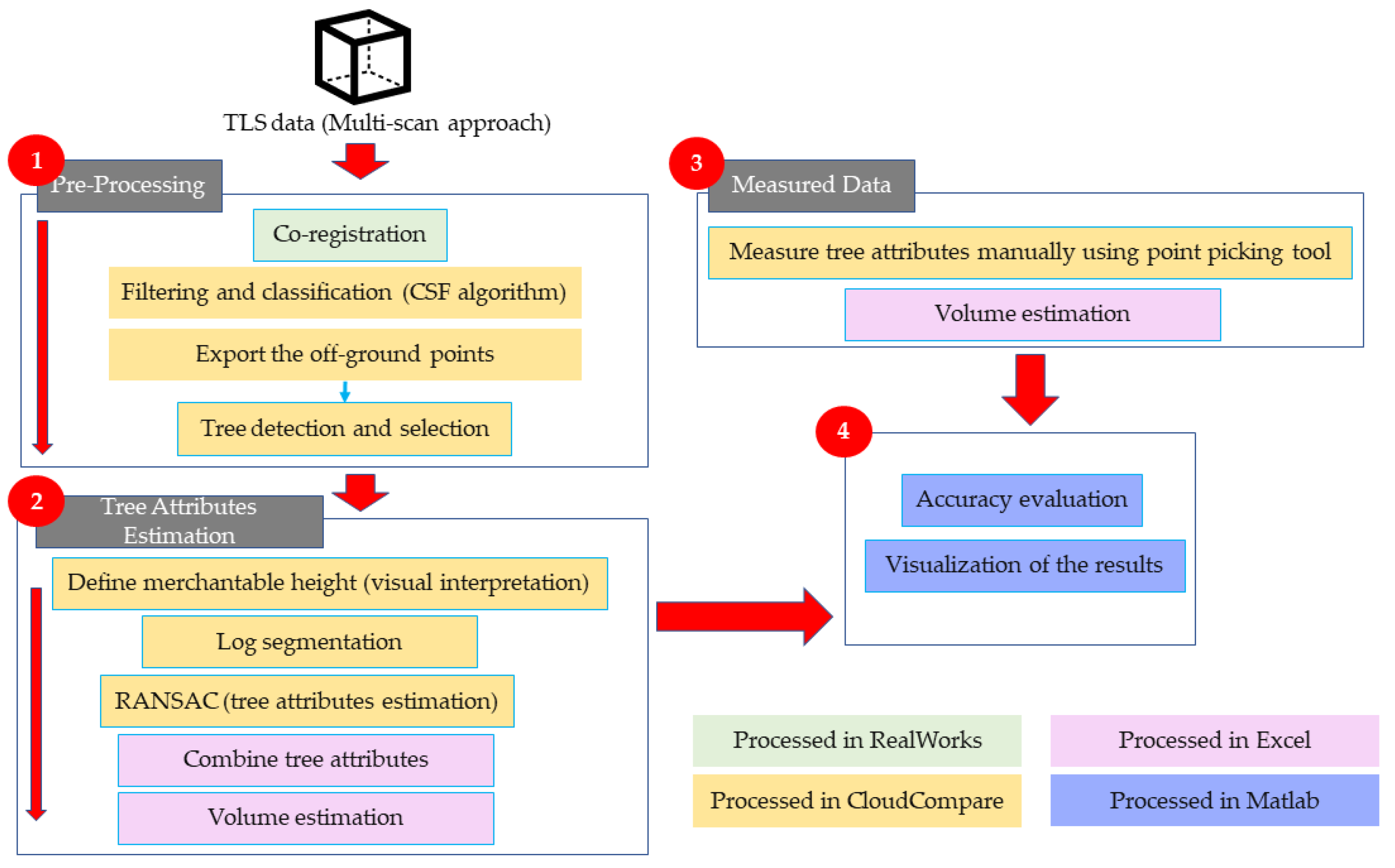
From Equations (11) and (12), is the measured value, is the average of the estimated values, and n is the number of observations. The entire validation process was conducted in Matlab R2017b. An illustration of the methodology is summarized in Figure 6.
3. Results and Discussion
3.1. Considering the Full Merchantable Length
This study aimed at expanding our current capabilities to estimate merchantable stem volume directly from TLS-based point clouds. As shown in a study and by Liang et al. [37], the utilization of a multi-scan approach from TLS ensures the construction of highly accurate tree models for the estimation of the most important tree attributes. Full coverage of the targeted trees by the point cloud data and minimizing occlusions can significantly reduce the estimated volumetric error (<10%).
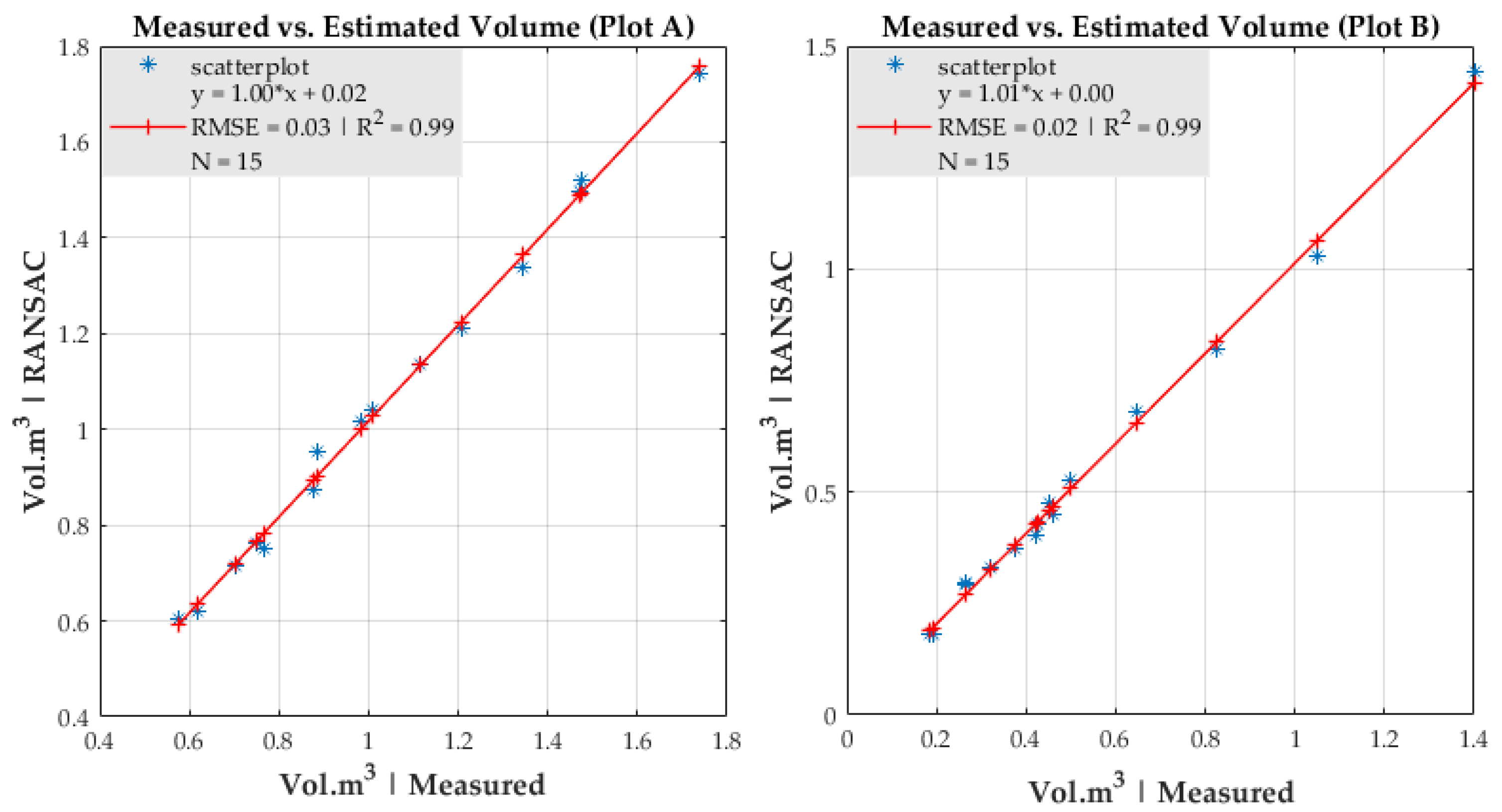
According to the regression analysis, the estimated merchantable volume was identical to the measured merchantable volume. For both plots, the R-squared results and the measured versus estimated volumetric values were highly correlated with R2 = 0.99 and RMSE = 0.03 for plot A, and R2 = 0.99 and RMSE = 0.02 for plot B (Figure 7 and Figure 8). Similarly, Mayamanikandan et al. [38] used the RANSAC algorithm on TLS point cloud data to compare the reliability of volume estimates. They obtained an R2 of 0.96, indicating good accordance with the field measurements. Based on the paired t-test for plot A (deciduous), there were statistically significant differences between measured and estimated merchantable volumes. In contrast, there were no statistically significant differences for plot B (coniferous) based on the Wilcoxon signed-rank test (Figure 8), which is consistent with a previous study we conducted [8].
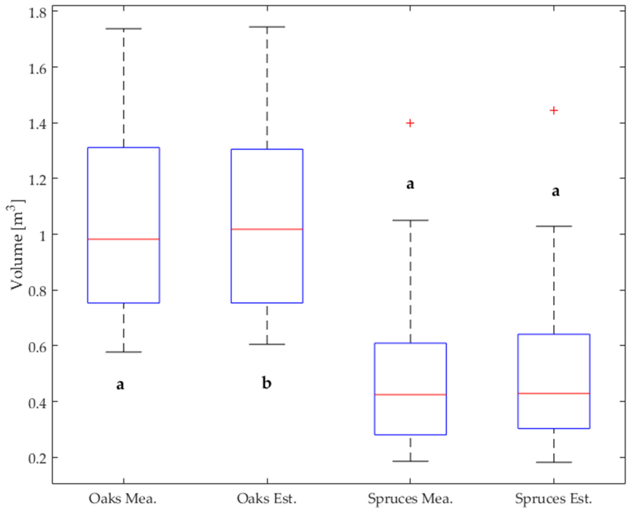
As evident in Figure 8 and Table 1, the RANSAC method slightly overestimated the merchantable volume in both plots. Our findings are in agreement with those from Olofsson et al. [27], who reported an overestimation of values in both deciduous trees and conifers. One reason for this overestimation can be branches. However, according to the Wilcoxon signed-rank test the difference was rather negligible and insignificant in the case of plot B with asymptotic significance (2-tailed) of 0.191 (Table 2). We assumed that this overestimation was likely related to the length of the selected logs (more details are given in Section 3.2). As described earlier, the higher the degree of stem curvature the higher the number of logs. In the case of plot B, the (i) number of selected logs was smaller and (ii) the lengths were longer compared with plot A.
Despite the shorter log length in plot A, a paired t-test indicated a significant difference between the measured and estimated merchantable volumes with a p-value of 0.0080 (Figure 8 and Table 3). It is likely that the higher level of structural complexity of the deciduous tree stems yielded higher bias estimations. Consequently, we also evaluated if a correlation existed between the length of the logs and the volume residuals (Figure 9) (more details are given in Section 3.2).
Although the validation metrics for merchantable volume showed higher accuracy for plot A compared with plot B (Table 3 and Table 4), the paired t-test revealed a significant difference between the measured and estimated volumes. As evident in Table 4, validation metrics showed a higher bias in plot A. In other words, the relationship (R2 = 0.99; RMSE = 0.03) found between estimated and measured merchantable volumes of plot A was purely random, which means that repeating this method in a different sample set (deciduous) would not guarantee the same accuracy and performance (Figure 7). The high agreement between estimated and measured merchantable volumes is consistent with the results from [18].
3.2. Considering Individual Logs
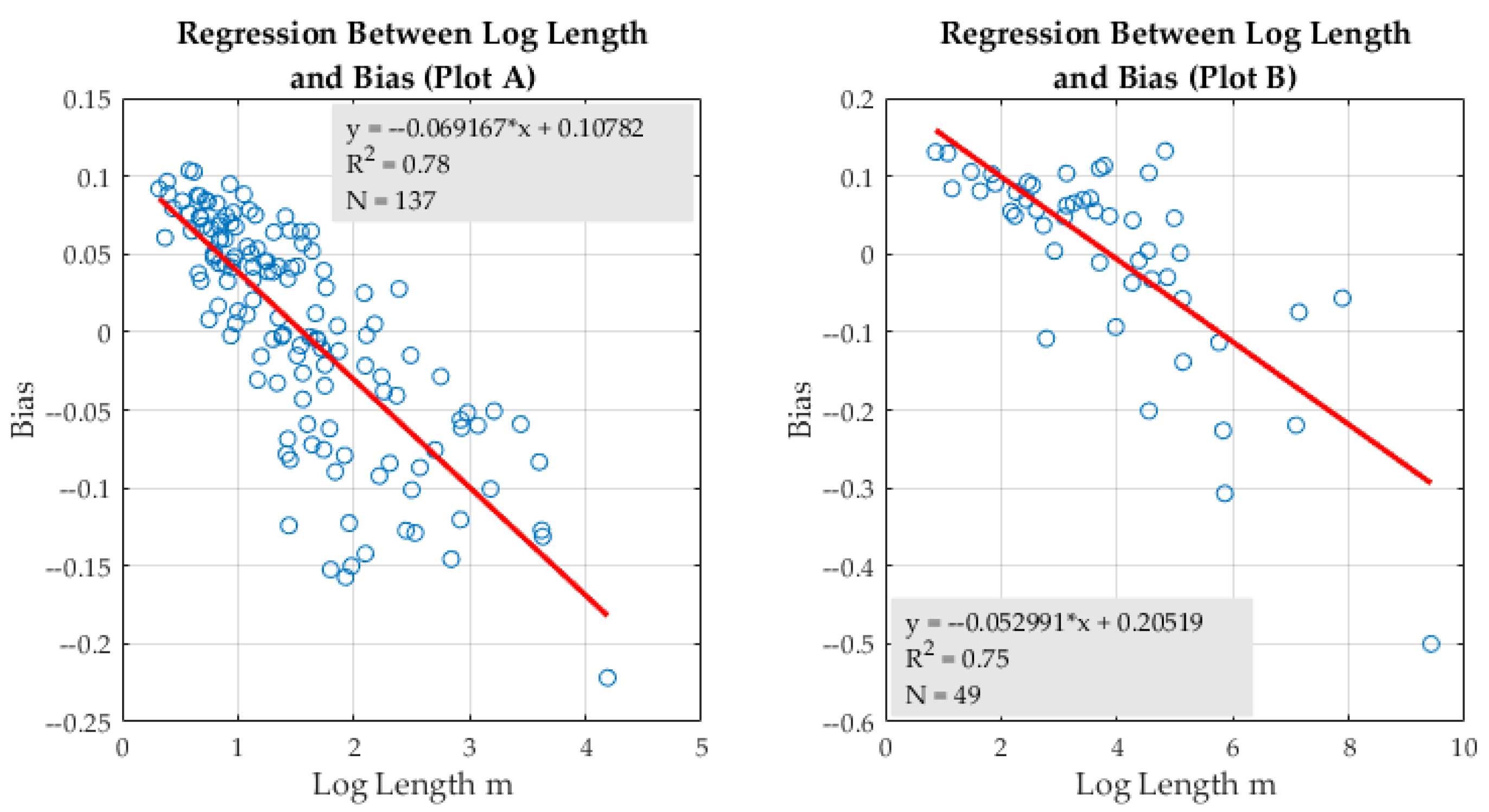
To evaluate the impact of log length on the estimation performance, we used a regression analysis and Spearman’s ρ correlation (Table 5). We observed a significant relationship between log lengths and bias; as calculated for each individual log, there was a correlation coefficient of −0.814 in plot A and −0.698 for plot B. Our results indicate that the longer the length of the log, the higher the bias; that is, it caused higher bias in a negative direction, which is translated to an overestimation of the estimated merchantable volume. As evident in Figure 9, with longer log lengths there was an overestimation in the amount of estimated merchantable volume (minus bias).
We also observed a significant correlation between log diameters and bias, with a bias of −0.618 for estimated and −0.617 for measured volumes in plot A, and −0.635 for estimated and −0.658 for measured volumes in plot B. This finding indicated that the larger the diameter, the greater the bias in a negative direction (Table 5). In other words, overestimation was evident in logs with larger diameters and underestimation in logs with smaller diameters (Table 5).
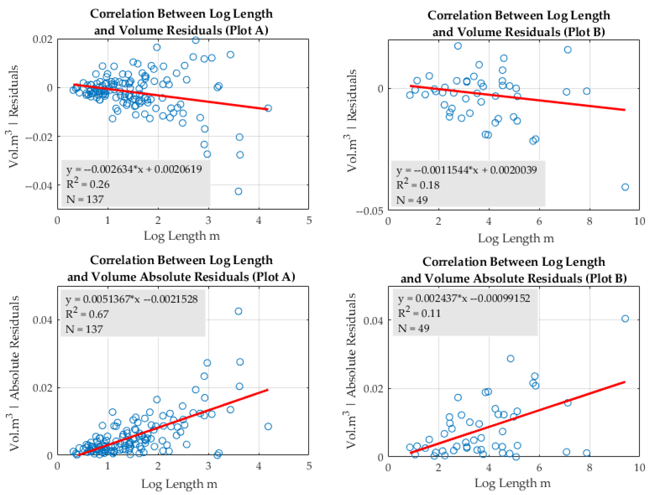
Finally, evaluating the correlation between absolute residuals and log attributes showed a similar tendency, meaning that the longer the length of the log, the higher the value of the absolute residuals (Figure 10), with a correlation coefficient of 0.61 for plot A and 0.367 for plot B (positive relationships). Figure 10 shows the amount of underestimation and overestimation using different log lengths and volume residuals.
However, in plot A there was no significant relationship between the absolute residuals and measured (p-value = 0.23) or estimated diameters (p-value = 0.157). In contrast, in plot B there was a moderate significant relationship between the absolute residuals and measured (correlation coefficient: 0.332, p-value = 0.02) and estimated diameters (correlation coefficient: 0.354, p-value = 0.012), which indicated that the larger the diameter, the higher the value of the absolute residuals (Table 5). In line with these results, a similar study conducted in Spain by Pérez-Martín et al. [39], using mobile laser scanning (MLS), showed higher residuals in stems with larger diameters. More specifically, they found a lower error in logs with a diameter <25 cm and a higher error with a diameter >50 cm.
Study limitations can exist due to technical constraints; for example, for estimating smaller logs with high precision, very high-resolution scans, instruments with small beam divergence, and a small (~10 m) scan position grid are required [40]. The occlusion effects in the higher stem portions of individual trees from TLS-based point clouds in complex forest conditions can lead to bias estimations [2,15].
4. Conclusions
We presented a method that provides reliable estimates for merchantable timber volume, as tested on commercial tree species. One of the main advantages of this methodology is that tree cutting is not required, nor is there a necessity for stem diameter measurements and additional silvicultural treatments in the field [41]. Merchantable height and diameter at any height along the stem can be estimated with high accuracy directly from tree-level remote sensing data. We estimated log lengths and diameters on standing trees simultaneously using the RANSAC method. This method provided higher elasticity in measurements compared with more traditional methods (e.g., relascope).
Our findings suggested that RANSAC performed very well for both plots in detecting and geometrically fitting the logs, not only in the event of the absence of pruned branches (lower tree portions) but also in cases where significant numbers of branches were present around the stems (Figure 4 and Figure 5), thus providing a robust and reliable approach for the extraction and estimation of key forest inventory attributes needed for the estimation of merchantable stem volumes. The proposed methodology resulted in a high degree of accuracy in both deciduous (97.73%) and conifer (96.14%) trees, respectively.
In conclusion, we may say that the larger the log, the higher the estimated bias. As our results indicated, the proposed method (RANSAC) had a higher impact on the accuracy of log lengths compared with the diameter of the logs. Therefore, it is highly recommended to divide the logs as much as possible into shorter lengths. This insight is critical because it can be used for the determination of log length selection in different stem portions. More specifically, in the case of oaks, we propose using 1 m log lengths for the lower portions of the stem, where the diameter is larger (e.g., larger than 25 cm) and 2 m for the upper portions of the stem where the diameter is smaller. For conifers, we suggest the use of 2 m log lengths for the lower portions (e.g., larger than 20 cm) and 4 m for the upper portions of the stem. Using these suggested log lengths, we can decrease the residual values and degree of bias (close to zero). In future work, we intend to maximize the commercial value of the suggested methodology by creating a code that can analyze the stem curvature changes at different heights, evaluate log quality and estimate log properties (e.g., length, diameter), to fully automate the process of merchantable volume estimation.
Supplementary Materials
The following are available online at https://0-www-mdpi-com.brum.beds.ac.uk/article/10.3390/rs13183610/s1, Table S1: RANSAC used parameters in CloudCompare.
Author Contributions
Conceptualization, D.P.; Methodology, D.P. and A.A.; Software, D.P. and A.A.; Validation, D.P. and A.A.; Formal analysis, D.P. and A.A.; Data curation, D.P and A.A.; Writing—original draft preparation, D.P. and A.A.; Writing—review and editing, D.P. and A.A.; Visualization, D.P. and A.A.; Supervision, D.P. and A.A. All authors have read and agreed to the published version of the manuscript.
Funding
This study was financially supported by EVA4.0 “Advanced Research Supporting the Forestry and Wood-processing Sector’s Adaptation to Global Change and the 4th Industrial Evolution” from the grant OPRDE (Project No. CZ.02.1.01/0.0/0.0/16_019/0000803) of the Faculty of Forestry and Wood Sciences (FFWS) from the Czech University of Life Sciences (CULS) in Prague.
Data Availability Statement
Restrictions apply to the availability of these data. Data were obtained from the Department of Forest Management; Faculty of Forestry and Wood Sciences of the Czech University of Life Sciences Prague and they are available from the authors with the permission of the Czech University of Life Sciences Prague.
Acknowledgments
We acknowledge that this study was financially supported by EVA4.0 “Advanced Research Supporting the Forestry and Wood-processing Sector’s Adaptation to Global Change and the 4th Industrial Evolution” from the grant OPRDE (Project No. CZ.02.1.01/0.0/0.0/16_019/0000803) of the Faculty of Forestry and Wood Sciences (FFWS) from the Czech University of Life Sciences (CULS) in Prague. We would also like to thank Martin Slavík from the department of Forest Management of the Faculty of Forestry and Wood Sciences (FFWS) from the Czech University of Life Sciences (CULS) in Prague for his contribution to the collection of TLS data.
Conflicts of Interest
The authors declare no conflict of interest.
References
- Bauwens, S.; Bartholomeus, H.; Calders, K.; Lejeune, P. Forest Inventory with Terrestrial LiDAR: A Comparison of Static and Hand-Held Mobile Laser Scanning. Forests 2016, 7, 127. [Google Scholar] [CrossRef] [Green Version]
- Sun, Y.; Liang, X.; Liang, Z.; Welham, C.; Li, W. Deriving Merchantable Volume in Poplar through a Localized Tapering Function from Non-Destructive Terrestrial Laser Scanning. Forests 2016, 7, 87. [Google Scholar] [CrossRef]
- Wang, Y.; Lehtomäki, M.; Liang, X.; Pyörälä, J.; Kukko, A.; Jaakkola, A.; Liu, J.; Feng, Z.; Chen, R.; Hyyppä, J. Is field-measured tree height as reliable as believed—A comparison study of tree height estimates from field measurement, airborne laser scanning and terrestrial laser scanning in a boreal forest. ISPRS J. Photogramm. Remote Sens. 2019, 147, 132–145. [Google Scholar] [CrossRef]
- Wang, Y.; Pyörälä, J.; Liang, X.; Lehtomäki, M.; Kukko, A.; Yu, X.; Kaartinen, H.; Hyyppä, J. In situ biomass estimation at tree and plot levels: What did data record and what did algorithms derive from terrestrial and aerial point clouds in boreal forest. Remote Sens. Environ. 2019, 232, 111309. [Google Scholar] [CrossRef]
- Forsman, M.; Börlin, N.; Holmgren, J. Estimation of tree stem attributes using terrestrial photogrammetry with a camera rig. Forests 2016, 7, 61. [Google Scholar] [CrossRef]
- Kalliovirta, J.; Laasasenaho, J.; Kangas, A. Evaluation of the laser-relascope. For. Ecol. Manag. 2005, 204, 181–194. [Google Scholar] [CrossRef]
- Stereńczak, K.; Mielcarek, M.; Wertz, B.; Bronisz, K.; Zajączkowski, G.; Jagodziński, A.M.; Ochał, W.; Skorupski, M. Factors influencing the accuracy of ground-based tree height measurements for major European tree species. J. Environ. Manag. 2019, 231, 1284–1292. [Google Scholar] [CrossRef]
- Panagiotidis, D.; Abdollahnejad, A.; Slavík, M. Assessment of Stem Volume on Plots Using Terrestrial Laser Scanner: A Precision Forestry Application. Sensors 2021, 21, 301. [Google Scholar] [CrossRef]
- Gaffrey, D.; Sloboda, B.; Matsumura, N. Representation of tree stem taper curves and their dynamic, using a linear model and the centroaffine transformation. J. For. Res. 1998, 3, 67–74. [Google Scholar] [CrossRef]
- Gong, J.R.; Zhang, X.S.; Huang, Y.M. Comparison of the performance of several hybrid poplar clones and their potential suitability for use in northern China. Biomass Bioenerg. 2011, 35, 2755–2764. [Google Scholar] [CrossRef]
- Chao, L.; Barclay, H.; Huang, S.M.; Hans, H.; Ghebremusse, S. Sensitivity of predictions of merchantable tree height, log production, and lumber recovery to tree taper. For. Chron. 2013, 89, 741–752. [Google Scholar]
- Rodríguez, F. Additively on nonlinear stem taper functions: A case for Corsican pine in Northern Spain. For. Sci. 2013, 59, 464–471. [Google Scholar]
- Subedi, N.; Sharma, M. Evaluating height–age determination methods for jack pine and black spruce plantations using stem analysis data. North. J. Appl. For. 2010, 27, 50–55. [Google Scholar] [CrossRef] [Green Version]
- Zhou, J.; Zhang, Z.Q.; Sun, G.; Fang, X.R.; Zha, T.G.; McNulty, S.; Chen, J.Q. Response of ecosystem carbon fluxes to drought events in a poplar plantation in Northern China. For. Ecol. Manag. 2013, 300, 33–42. [Google Scholar] [CrossRef]
- Panagiotidis, D.; Surový, P.; Kuželka, K. Accuracy of Structure from Motion models in comparison with terrestrial laser scanner for the analysis of DBH and height influence on error behaviour. J. For. Sci. 2016, 62, 357–365. [Google Scholar] [CrossRef] [Green Version]
- Cabo, C.; Del Pozo, S.; Rodríguez-Gonzálvez, P.; Ordóñez, C.; González-Aguilera, D. Comparing Terrestrial Laser Scanning (TLS) and Wearable Laser Scanning (WLS) for Individual Tree Modeling at Plot Level. Remote Sens. 2018, 10, 540. [Google Scholar] [CrossRef] [Green Version]
- Liu, G.; Wang, J.; Dong, P.; Chen, Y.; Liu, Z. Estimating Individual Tree Height and Diameter at Breast Height (DBH) from Terrestrial Laser Scanning (TLS) Data at Plot Level. Forests 2018, 9, 398. [Google Scholar] [CrossRef] [Green Version]
- Dassot, M.; Colin, A.; Santenoise, P.; Fournier, M.; Constant, T. Terrestrial laser scanning for measuring the solid wood volume, including branches, of adult standing trees in the forest environment. Electron. Agricult. 2012, 89, 86–93. [Google Scholar] [CrossRef]
- Iizuka, K.; Hayakawa, Y.S.; Ogura, T.; Nakata, Y.; Kosugi, Y.; Yonehara, T. Integration of Multi-Sensor Data to Estimate Plot-Level Stem Volume Using Machine Learning Algorithms–Case Study of Evergreen Conifer Planted Forests in Japan. Remote Sens. 2020, 12, 1649. [Google Scholar] [CrossRef]
- Panagiotidis, D.; Abdollahnejad, A. Accuracy Assessment of Total Stem Volume Using Close-Range Sensing: Advances in Precision Forestry. Forests 2021, 12, 717. [Google Scholar] [CrossRef]
- Momo Takoudjou, S.; Ploton, P.; Sonké, B.; Hackenberg, J.; Griffon, S.; De Coligny, F.; Kamdem, N.G.; Libalah, M.; Mofack, G.I.I.; Le Moguédec, G.; et al. Using terrestrial laser scanning data to estimate large tropical trees biomass and calibrate allometric models: A comparison with traditional destructive approach. Methods Ecol. Evol. 2018, 9, 905–916. [Google Scholar] [CrossRef]
- Gonzalez de Tanago, J.; Lau, A.; Bartholomeus, H.; Herold, M.; Avitabile, V.; Raumonen, P.; Martius, C.; Goodman, R.C.; Disney, M.; Manuri, S. Estimation of above-ground biomass of large tropical trees with terrestrial LiDAR. Methods Ecol. Evol. 2018, 9, 223–234. [Google Scholar] [CrossRef] [Green Version]
- Lau, A.; Bentley, L.P.; Martius, C.; Shenkin, A.; Bartholomeus, H.; Raumonen, P.; Malhi, Y.; Jackson, T.; Herold, M. Quantifying branch architecture of tropical trees using terrestrial LiDAR and 3D modelling. Trees 2018, 32, 1219–1231. [Google Scholar] [CrossRef] [Green Version]
- Fernández-Sarría, A.; Velázquez-Martí, B.; Sajdak, M.; Martínez, L.; Estornell, J. Residual biomass calculation from individual tree architecture using terrestrial laser scanner and groundlevel measurements. Comput. Electron. Agric. 2013, 93, 90–97. [Google Scholar] [CrossRef]
- Yrttimaa, T.; Saarinen, N.; Luoma, V.; Tanhuanpaa, T.; Kankare, V.; Liang, X.L.; Hyyppa, J.; Holopainen, M.; Vastaranta, M. Detecting and characterizing downed dead wood using terrestrial laser scanning. ISPRS J. Photogramm. Remote Sens. 2019, 151, 76–90. [Google Scholar] [CrossRef]
- Amiri, N.; Polewski, P.; Yao, W.; Krzystek, P.; Skidmore, A.K. Detection of Single Tree Stems in Forested Areas from High Density ALS Point Clouds Using 3d Shape Descriptors. In Proceedings of the ISPRS Annals of the Photogrammetry, Remote Sensing and Spatial Information Sciences, Wuhan, China, 18–22 September 2017; Volume IV-2/W4, pp. 35–42. [Google Scholar] [CrossRef] [Green Version]
- Olofsson, K.; Holmgren, J.; Olsson, H. Tree Stem and Height Measurements using Terrestrial Laser Scanning and the RANSAC Algorithm. Remote Sens. 2014, 6, 4323–4344. [Google Scholar] [CrossRef] [Green Version]
- Yang, B.; Zang, Y. Automated registration of dense terrestrial laser-scanning point clouds using curves. ISPRS J. Photogramm. Remote Sens. 2014, 3, 109–121. [Google Scholar] [CrossRef]
- Chen, C.; Yang, B. Dynamic occlusion detection and inpainting of in situ captured terrestrial laser scanning point clouds sequence. ISPRS J. Photogramm. Remote Sens. 2016, 119, 90–107. [Google Scholar] [CrossRef]
- Chen, S.; Liu, H.; Feng, Z.; Shen, C.; Chen, P. Applicability of personal laser scanning in forestry inventory. PLoS ONE 2019, 14, e0211392. [Google Scholar] [CrossRef] [PubMed]
- Trimble RealWorks 10.2 User Guide. 2017. Available online: https://www.trimble.com/3d-laser-scanning/realworks.aspx (accessed on 12 October 2019).
- Girardeau-Montaut, D. Cloud Compare. 2017. Available online: http://www.danielgm.org (accessed on 19 December 2016).
- Zhang, W.; Qi, J.; Wan, P.; Wang, H.; Xie, D.; Wang, X.; Yan, G. An Easy-to-Use Airborne LiDAR Data Filtering Method Based on Cloth Simulation. Remote Sens. 2016, 8, 501. [Google Scholar] [CrossRef]
- Gschwantner, T.; Alberdi, I.; Balázs, A.; Bauwens, S.; Bender, S.; Borota, D.; Bosela, M.; Bouriaud, O.; Cañellas, I.; Donis, J.; et al. Harmonisation of stem volume estimates in European National Forest Inventories. Ann. For. Sci. 2019, 76, 24. [Google Scholar] [CrossRef] [Green Version]
- Schnabel, R.; Wahl, R.; Klein, R. Efficient RANSAC for point-cloud shape detection. Comput. Graph. Forum 2007, 26, 214–226. [Google Scholar] [CrossRef]
- Baronti, L.; Alston, M.; Mavrakis, N.; Ghalamzan, E.A.M.; Castellani, M. Primitive Shape Fitting in Point Clouds Using the Bees Algorithm. Appl. Sci. 2019, 9, 5198. [Google Scholar] [CrossRef] [Green Version]
- Liang, X.; Kankare, V.; Hyyppä, J.; Wang, Y.; Kukko, A.; Haggrén, H.; Yu, X.; Kaartinen, H.; Jaakkola, A.; Guan, F.; et al. Terrestrial laser scanning in forest inventories. ISPRS J. Photogramm. Remote Sens. 2016, 115, 63–77. [Google Scholar] [CrossRef]
- Mayamanikandan, T.; Reddy, R.S.; Jha, C. Non-Destructive Tree Volume Estimation using Terrestrial Lidar Data in Teak Dominated Central Indian Forests. In Proceedings of the 2019 IEEE Recent Advances in Geoscience and Remote Sensing: Technologies, Standards and Applications (TENGARSS), Kochi, India, 17–20 October 2019; pp. 100–103. [Google Scholar]
- Pérez-Martín, E.; López-Cuervo Medina, S.; Herrero-Tejedor, T.; Pérez-Souza, M.A.; Aguirre de Mata, J.; Ezquerra-Canalejo, A. Assessment of Tree Diameter Estimation Methods from Mobile Laser Scanning in a Historic Garden. Forests 2021, 12, 1013. [Google Scholar] [CrossRef]
- Wilkes, P.; Lau, A.; Disney, M.; Calders, K.; Burt, A.; De Tanago, J.G.; Bartholomeus, H.; Brede, B.; Herold, M. Data acquisition considerations for terrestrial laser scanning of forest plots. Remote Sens. Environ. 2017, 196, 140–153. [Google Scholar] [CrossRef]
- Vaaja, M.T.; Virtanen, J.-P.; Kurkela, M.; Lehtola, V.; Hyyppä, J.; Hyyppä, H. The effect of wind on tree stem parameter estimation using terrestrial laser scanning. ISPRS Ann. Photogramm. Remote Sens. Spat. Inf. Sci. 2016, 8, 117–122. [Google Scholar] [CrossRef] [Green Version]
Figure 1.
Map of Czechia, including the geographic locations of the two study areas. We used the coordinate system WGS 1984 Web Mercator (auxiliary sphere).
Figure 1.
Map of Czechia, including the geographic locations of the two study areas. We used the coordinate system WGS 1984 Web Mercator (auxiliary sphere).

Figure 2.
(a,b) Examples showing the use of visual interpretation for the determination of cut off height for forked trees (plot A), and (c) use of upper diameter limit of 19 cm for the determination of the cut off height (plot B).
Figure 2.
(a,b) Examples showing the use of visual interpretation for the determination of cut off height for forked trees (plot A), and (c) use of upper diameter limit of 19 cm for the determination of the cut off height (plot B).

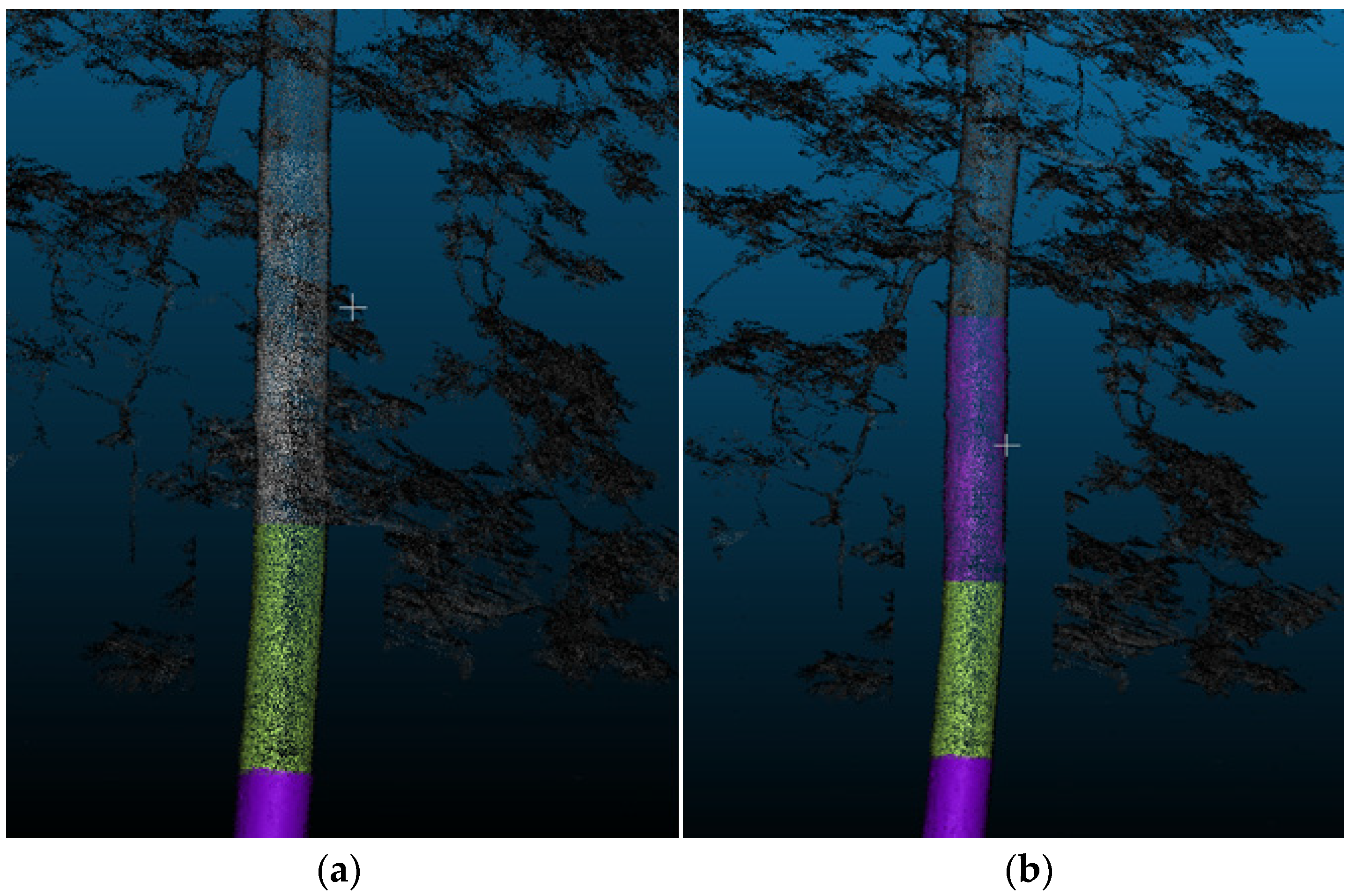
Figure 3.
(a) Example of log segment (open brown color) on deciduous tree (plot A) including fuzzy selection of branch leaves, and (b) selection of log points (purple color) for direct use of the RANSAC algorithm (without any additional point cloud processing, e.g., branch removal), demonstrating the high degree of tolerance and performance of the algorithm on data with large numbers of outliers.

Figure 4.
(a,b) Example of a coniferous log, showing the estimated values (log length and diameter) using the RANSAC method directly applied to the stem.
Figure 4.
(a,b) Example of a coniferous log, showing the estimated values (log length and diameter) using the RANSAC method directly applied to the stem.

Figure 5.
Example of length and diameter measurements from a segmented log. The diameter extraction was based on two perpendicular measurements (red color).
Figure 5.
Example of length and diameter measurements from a segmented log. The diameter extraction was based on two perpendicular measurements (red color).

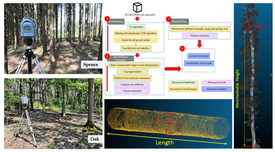
Figure 6.
A flow chart to illustrate the analysis and outputs.

Figure 7.
Linear regression models of the measured and estimated merchantable volume.

Figure 8.
Box-and-whisker plots of the measured and estimated merchantable volumes. The letters (a and b) indicate if there were significant differences between the measured and estimated merchantable volumes at a 0.05 significance level. The red plus signs represents outliers.
Figure 8.
Box-and-whisker plots of the measured and estimated merchantable volumes. The letters (a and b) indicate if there were significant differences between the measured and estimated merchantable volumes at a 0.05 significance level. The red plus signs represents outliers.

Figure 9.
Linear regression models between log lengths and bias.

Figure 10.
Shows the correlation between the log length and the produced volume residuals and absolute residuals.
Figure 10.
Shows the correlation between the log length and the produced volume residuals and absolute residuals.


Table 1.
Summary table of descriptive statistics of merchantable volume in m3.
| Plot A | Plot B | |||
|---|---|---|---|---|
| Measured | Estimated | Measured | Estimated | |
| N | 15 | 15 | 15 | 15 |
| Range | 1.16 | 1.14 | 1.21 | 1.26 |
| Minimum | 0.58 | 0.61 | 0.19 | 0.18 |
| Maximum | 1.74 | 1.74 | 1.40 | 1.44 |
| Mean | 1.03 | 1.05 | 0.52 | 0.53 |
| Standard Error Mean | 0.09 | 0.09 | 0.09 | 0.09 |
| Standard Deviation | 0.35 | 0.35 | 0.34 | 0.34 |
| Variance | 0.12 | 0.12 | 0.11 | 0.12 |
| Skewness | 0.57 | 0.54 | 1.59 | 1.64 |
| Skewness Standard Error | 0.58 | 0.58 | 0.58 | 0.58 |
| Kurtosis | −0.62 | −0.68 | 2.32 | 2.71 |
| Kurtosis Standard Error | 1.12 | 1.12 | 1.12 | 1.12 |
Table 2.
Wilcoxon signed-rank test (plot B).
| Negative Ranks | Positive Ranks | Z | Asymp. Sig. (2-Tailed) |
|---|---|---|---|
| 7.0000 | 8.0000 | −1.306 * | 0.191 |
Negative Rank: Estimated < Measured. Positive Rank: Measured > Estimated. * Based on positive ranks.
Table 3.
Paired t-test results (plot A).
| Mean | Standard Deviation | Standard Error Mean | 95% CID 1 | t | df | Sig. (2-Tailed) | |
|---|---|---|---|---|---|---|---|
| Lower | Upper | ||||||
| −0.0177 | 0.0221 | 0.0057 | −0.0299 | −0.0055 | −3.1040 | 14 | 0.0080 |
1 Confidence Interval of the Difference.
Table 4.
Statistical summary of validation metrics.
| Metric | Plot A | Plot B | Metric | Plot A | Plot B |
|---|---|---|---|---|---|
| MAD | 0.02 | 0.02 | MAPE | 2.27 | 3.86 |
| MSE | 0.00 | 0.00 | BIAS | 0.02 | 0.01 |
| RMSE | 0.03 | 0.02 | BIAS% | 1.68 | 1.49 |
| RMSE% | 2.68 | 4.09 | MAE | 0.02 | 0.02 |
| % of accuracy | 97.73 | 96.14 | N | 15.00 | 15.00 |
Table 5.
Summary table of Spearman correlation results (two-tailed).
| Length | Estimated Diameter | Measured Diameter | |||||
|---|---|---|---|---|---|---|---|
| CC 1 | Sig. | CC 1 | Sig. | CC 1 | Sig. | ||
| Plot A | Bias | −0.814 | 0 | −0.618 | 0 | −0.617 | 0 |
| Absolute Residuals | 0.610 | 0 | 0.122 | 0.157 | 0.103 | 0.23 | |
| Plot B | Bias | −0.698 | 0 | −0.635 | 0 | −0.658 | 0 |
| Absolute Residuals | 0.367 | 0.009 | 0.354 | 0.012 | 0.332 | 0.02 | |
1 Correlation Coefficient.
Publisher’s Note: MDPI stays neutral with regard to jurisdictional claims in published maps and institutional affiliations. |
© 2021 by the authors. Licensee MDPI, Basel, Switzerland. This article is an open access article distributed under the terms and conditions of the Creative Commons Attribution (CC BY) license (https://creativecommons.org/licenses/by/4.0/).
Share and Cite
MDPI and ACS Style
Panagiotidis, D.; Abdollahnejad, A. Reliable Estimates of Merchantable Timber Volume from Terrestrial Laser Scanning. Remote Sens. 2021, 13, 3610. https://0-doi-org.brum.beds.ac.uk/10.3390/rs13183610
AMA Style
Panagiotidis D, Abdollahnejad A. Reliable Estimates of Merchantable Timber Volume from Terrestrial Laser Scanning. Remote Sensing. 2021; 13(18):3610. https://0-doi-org.brum.beds.ac.uk/10.3390/rs13183610
Chicago/Turabian StylePanagiotidis, Dimitrios, and Azadeh Abdollahnejad. 2021. "Reliable Estimates of Merchantable Timber Volume from Terrestrial Laser Scanning" Remote Sensing 13, no. 18: 3610. https://0-doi-org.brum.beds.ac.uk/10.3390/rs13183610
Note that from the first issue of 2016, this journal uses article numbers instead of page numbers. See further details here.