
Dual-Weighted Kernel Extreme Learning Machine for Hyperspectral Imagery Classification


1
School of Electronics and Information Engineering, Northwestern Polytechnical University, Xi’an 710072, China
2
School of Electronics and Information Engineering, Shaoguan University, Shaoguan 512023, China
*
Author to whom correspondence should be addressed.
Remote Sens. 2021, 13(3), 508; https://0-doi-org.brum.beds.ac.uk/10.3390/rs13030508
Submission received: 9 November 2020
/
Revised: 17 January 2021
/
Accepted: 28 January 2021
/
Published: 1 February 2021
(This article belongs to the Special Issue Classification and Feature Extraction Based on Remote Sensing Imagery)
Abstract
:Due to its excellent performance in high-dimensional space, the kernel extreme learning machine has been widely used in pattern recognition and machine learning fields. In this paper, we propose a dual-weighted kernel extreme learning machine for hyperspectral imagery classification. First, diverse spatial features are extracted by guided filtering. Then, the spatial features and spectral features are composited by a weighted kernel summation form. Finally, the weighted extreme learning machine is employed for the hyperspectral imagery classification task. This dual-weighted framework guarantees that the subtle spatial features are extracted, while the importance of minority samples is emphasized. Experiments carried on three public data sets demonstrate that the proposed dual-weighted kernel extreme learning machine (DW-KELM) performs better than other kernel methods, in terms of accuracy of classification, and can achieve satisfactory results.
1. Introduction
Hyperspectral remote sensing images contain rich spatial and spectral object information, including ultraviolet, visible, and near- and mid-infrared regions of electromagnetic waves. For this reason, the ability to recognize and classify ground objects has greatly improved. The classification of hyperspectral images has become a hot research topic in recent years, with a considerable amount of research on hyperspectral image classification having been conducted. However, despite the rich information provided by hyperspectral images, their high dimensionality and non-linear characteristics make detailed classification difficult. Moreover, as the number of available training samples is typically small, we previously encountered the Hughes phenomenon [1] during the supervised classification of hyperspectral images (HSI). To overcome the high-dimensionality problem, many methods have been introduced for HSI classification and shown good performance, such as manifold learning, the support vector machine (SVM) [2], and composite kernel-based methods [3,4,5,6,7].
Recently, many deep learning employed for hyperspectral imagery classification tasks. H.Wu [8] proposed semi-supervised deep learning for hyperspectral image classification, while the approach uses limited labeled data and abundant unlabeled data to train a deep neural network. B. Pan [9] introduced a dilated semantic segmentation network, in order to avoid spatial information loss during the pooling operation. The network has an end-to-end structure, thus reducing time consumption. In [10], a deep learning method by combining spatial and spectral information for HSI classification was successfully designed. An unsupervised spatial–spectral feature learning strategy using a 3-dimensional convolutional auto-encoder (3D-CAE) has been proposed for hyperspectral data [11]. The proposed 3D-CAE maximally explores the spatial–spectral structure information for feature extraction.
Sparse representation is also a commonly used method to hyperspectral image classification. J. Peng [12] designed a self-paced joint sparse representation model which replaces the least-squares loss in the standard joint sparse representation with a weighted least-squares loss and adopts a self-paced learning (SPL) strategy to learn the weights for neighboring pixels. In order to improve the robustness of joint sparse representation (JSR) [13], J. Peng proposed maximum likelihood estimation (MLE) based a JSR model, which replaces the traditional quadratic loss function with an MLE-like estimator to measure the joint approximation error by providing priors on the coding residuals. This model can easily be converted to an iteratively reweighted JSR problem. Y. Yuan [14] proposed a method that mainly focuses on multitask joint sparse representation (MJSR) and a stepwise Markov random field framework to tackle such problems.
As an effective strategy the multi-features have been widely used to improve the accuracy of classification. Y. Gu [15] proposed non-linear multiple kernel learning, which learned an optimal combined kernel from pre-defined linear base kernels. J. Li [16] constructed a new family of generalized composite kernels, which showed great flexibility in the way that they combined the spectral information contained in hyperspectral data without weighted parameters. W. Li [17] introduced the one-against-one strategy by using discriminant analysis within kernel-induced feature spaces. L. Fang [18] presented a novel framework to effectively utilize the spectral–spatial information of super pixels through multiple kernels, which extracted extinction profiles from three independent components and then created an adaptive composite kernel to explore the spatial information.
Compared to the above-mentioned methods, the extreme learning machine (ELM) [19] has received a lot more attention, due to its advantages. ELM does not need to tune the hidden layer parameters if the network architecture is determined. The hidden layer parameters in ELM are randomly generated and independent of the training data and application environments. By minimizing the training error and the norm of output weights simultaneously, ELM tends to have better generalization performance and provides a unified analytic solution to binary, multiclass, and regression problems. However, despite the advantages mentioned above, when an ELM is directly applied to a HSI data set, the accuracy is still not high, as only spectral information is used. Some methods combining spatial–spectral information based on ELM for HSI classification have been proposed. To evaluate the effectiveness of a kernel-based extreme learning machine algorithm, Pal, M. [20] applied the kernel ELM method to multispectral and hyperspectral remote-sensing data. The results suggested that the accuracy was similar to that of SVM, while it had a lower computation cost. For weighted summation form of kernel extreme learning model, Y. Zhou [21] proposed two spatial–spectral composite kernel ELM algorithms for HSI classification. C. Chen [22] exploited Gabor filtering and multi-hypothesis to extract spatial information, then used the joint spectral information as an ELM input. In [23], extended morphological profiles were employed for spatial information in ELM-based classification of HSI. M. Jiang [24] exploited a multiscale spatial weighted-mean filtering-based approach to extract multiple spatial information. F. Cao [25] proposed probabilistic modeling with a sparse representation and weighted composite features (WCFs) to derive the optimized output weights. Similarly as deep learning method, J. Li [26] proposed a new classification framework, derived from the deep KELM network, in which deep KELM was employed to generate deep spectral features. Ensemble learning based method was also developed for hyperspectral imagery classification, Ugur Ergul [27] proposed a new boosting-based algorithm, which enables the construction of composite kernels (CKs) by using spatial and spectral hybrid kernels. In [28], an improved hierarchical ELM was designed by adding an ELM to a hierarchical ELM. In this model, the average spectral-spatial features were extracted twice by this multiple layer framework; satisfactory results were achieved. As a kind of optimization a multiple reduced kernel extreme learning machine was introduced [29], with which the combination of hybrid kernels and optimal weights could be achieved, allowing the features of the hyperspectral image to be fully represented and the classification error rates to be reduced. As extended attribute profiles usually require manual parameter settings, Marpu [30] presented a technique to automatically produce the extended attribute profiles under consideration of the standard deviation, where the homogenous regions were retained by the minimum and maximum values of the standard deviation. Recently, group intelligent algorithms have also been used: H. Su [31,32] proposed an extreme learning machined optimized by the firefly algorithm, where the parameters in ELM were optimized by the proposed method. J. Li [33] presented an empirical linear relationship between the training number and hidden nodes with a linear model. To improve the individual performance of a basic classifier, F. Lv [34] proposed a stacked auto-encoder ELM (SAE-ELM) model. The features were extracted by this model, while the Q statistic was adopted to determine the final results. Spatial features provide subtle information, which helps discriminate different classes. As an excellent edge-preserving filter, guided image filtering [35], which was proposed by He, has been widely used in the fields of noise reduction, haze removal, and so on. B. Pan [36] proposed an ensemble framework where, by integrating many individual learners, better generation can be achieved. To establish the ensemble model, hierarchical guidance filtering was employed. Y. Guo [37] attempted to develop two fusion methods for spectral and spatial features and, in order to obtain better results, adopted guided image filtering. Z. Wang [38] proposed a discriminative guided filtering framework which integrates a classifier by guided filtering. Guided image filtering establishes a local linear model between the guided image and the output image, implicitly completes the filtering of the input image by solving the difference function between the input image and the output image [35,39]. Inspired by these studies, guided image filtering is used to extract spatial information, in order to further improve the accuracy of hyperspectral image classification (HSIC).
While these spatial–spectral ELM-based methods performed well, their performance can be further improved, as they ignored the imbalanced samples in different classes in multiclassification tasks, causing the majority of samples to weaken the minority’s influences on the classification performance; thus, small-sized samples should be taken into consideration. Motivated by these, we propose a dual weighted kernel extreme learning for hyperspectral image classification. For one thing, different scales of spatial features extend the feature space, the combination of multiscale spatial features will rich the diversity of samples which may bring more information for our classification task. The other, in imbalanced data environment, the separating boundary is supposed to be pushed toward the side of minority class, which in fact favors the performance of majority class. To alleviate the depression by the majority, we attempt to assign an extra weight to each sample to strengthen the impact of minorities and weaken the impact of majorities in some distant.
To tackle the above task, the main contributions of this paper are summarized below:
A spatial–spectral dual-weighted kernel extreme learning machine framework for hyperspectral image classification is proposed. As important spatial features can help to identify similar classes, the spatial- and spectral-added weight summation make hyperspectral imagery classification feasible. In addition, the minority class should not be ignored, as the majority classes may weaken the generalization performance of minorities. For this reason, the weighted extreme learning machine is employed, in order to counteract this imbalance problem.
The rest of the paper is organized as follows: In Section 2, the related works of single layer feed-forward networks, ELM and weighted kernel ELM, and guided filters are introduced; furthermore, the proposed dual-weighted kernel ELM is described in detail. The experimental results and analysis are provided in Section 3. The conclusions of this paper are given in Section 4.
2. Materials and Methods
2.1. Weighted Kernel Extreme Learning Machine
2.1.1. Single-Layer Feedforward Neural Networks (SLFN)
ELM is a fast-learning algorithm for single hidden layer neural networks, which works by randomly initializing the input weights and biases, which can greatly save a considerable amount of computation time. Meanwhile, the random input may bring diversity of samples.
For a single hidden layer neural network, we suppose that there are N arbitrary samples, , where and . Therefore, a single hidden layer neural network with one hidden layer node can be expressed as
where is the activation function, is the output weight, is the weight vector, and is the bias of the ith hidden layer.
G. Huang [19] proved that SLFN with L nodes can approximate an arbitrary function. Therefore, , and can satisfy , such that
We used the matrix form to rewrite Equation (2):
where and .
The hidden layer output matrix, is expressed as
The matrix is an active function of the hidden layer. In Equation (5), the parameters and are both unknown:
In traditional neural networks, Equation (5) is usually solved using a gradient descent-based iterative algorithm. During the process of iteration, all parameters need to be tuned, according to the iteration, which may cause the problems of gradient diffusion, local minima, and overfitting.
2.1.2. ELM and Weighted Kernel ELM
As for ELM, the solution of the parameters is completely different. The parameters and are randomly generated. They do not change during the whole procedure. The hidden layer is determined after the input parameters are produced. Based on the input parameter and hidden layer, we can derive the output by the linear analytic solution. The final goal of ELM is to obtain the smallest training error with the smallest norm of the output weight. This is expressed as
Based on optimization theory, Equation (6) can be formulated as follows:
where , is the training error, and is the regularization parameter.
According to Lagrange multiplier theory and Karush–Kuhn–Tucker (KKT) optimization conditions [40], training the ELM is equivalent to solving the following dual optimization problem:
where is the column vector of matrix β and is the Lagrange multiplier. From the KKT theorem, we can further derive:
Based on Equations (9)–(11), the output weight, , can be expressed as
After obtaining the output weight , the output of the ELM is obtained as:
Traditional ELM does not take the imbalance problem into account, while the weighted ELM was designed to address it [41]. For this paper, two weighting schemes were proposed:
Scheme 1:
where is the total number of samples belonging to the th class. After applying weighting scheme 1, we can obtain a balanced ratio between the minority and majority.
Scheme 2:
where represents the average number of samples for all classes. If the number of is below the average, similar to ELM, the optimization form of the weighted ELM can be expressed as:
For the multiclass-weighted kernel ELM [41,42], we define a diagonal matrix, , which is associated with the training sample The output weight, , can be expressed as
Given a new sample, , the output function of the weighted ELM classifier is obtained from , that is:
Similar to SVM kernel methods, the kernel trick can be used in Equation (18), where the kernel function can replace the inner products and .
The kernel trick version of the weighted ELM is the weighted kernel ELM. Thus, the version of the kernel ELM can be rewritten as:
where and .
Therefore, the weighted kernel ELM provides a unified solution for networks with different feature mappings and, at the same time, strengthens the impact of minority class samples by adding a weighted matrix.
2.2. Spatial Feature Extraction
To improve the performance of ELM for HSI classification, guided image filtering is adopted to extract spatial information. The guided image filtering method proposed by He [36] is a novel type of explicit filter that can act as an edge-preserving smoothing operator-like bilateral filter and obtain better behavior near edges. Given an image as an input, is a guided image, is an output image—which is a linear transform in a window around a pixel with a size of , where is the window radius—and is the pixel of :
where are linear coefficients that are assumed to be constant in . From Equation (20), we can see that , which means that the output has a similar gradient as the guidance image . The coefficients are solved by the following minimum cost function:
where is a regularization parameter, to prevent from being too large. The values of and can be obtained by linear regression [40]:
where and are the mean and variance of in the window of , is the number of pixels in , and is the mean of in . After obtaining the coefficients and , the guided filtering image can be computed. Based on the above procedure, we can obtain the linear transformed image .
2.3. Proposed Dual-Weighted Kernel ELM-Based Method
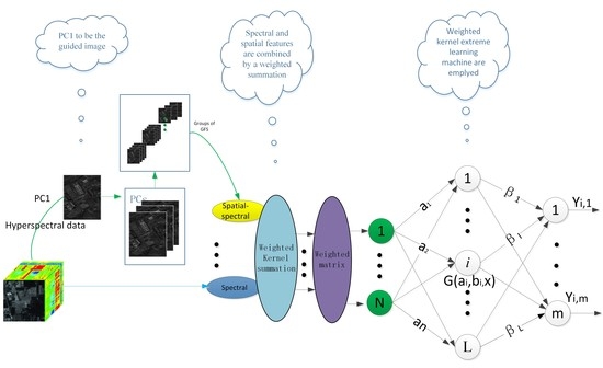
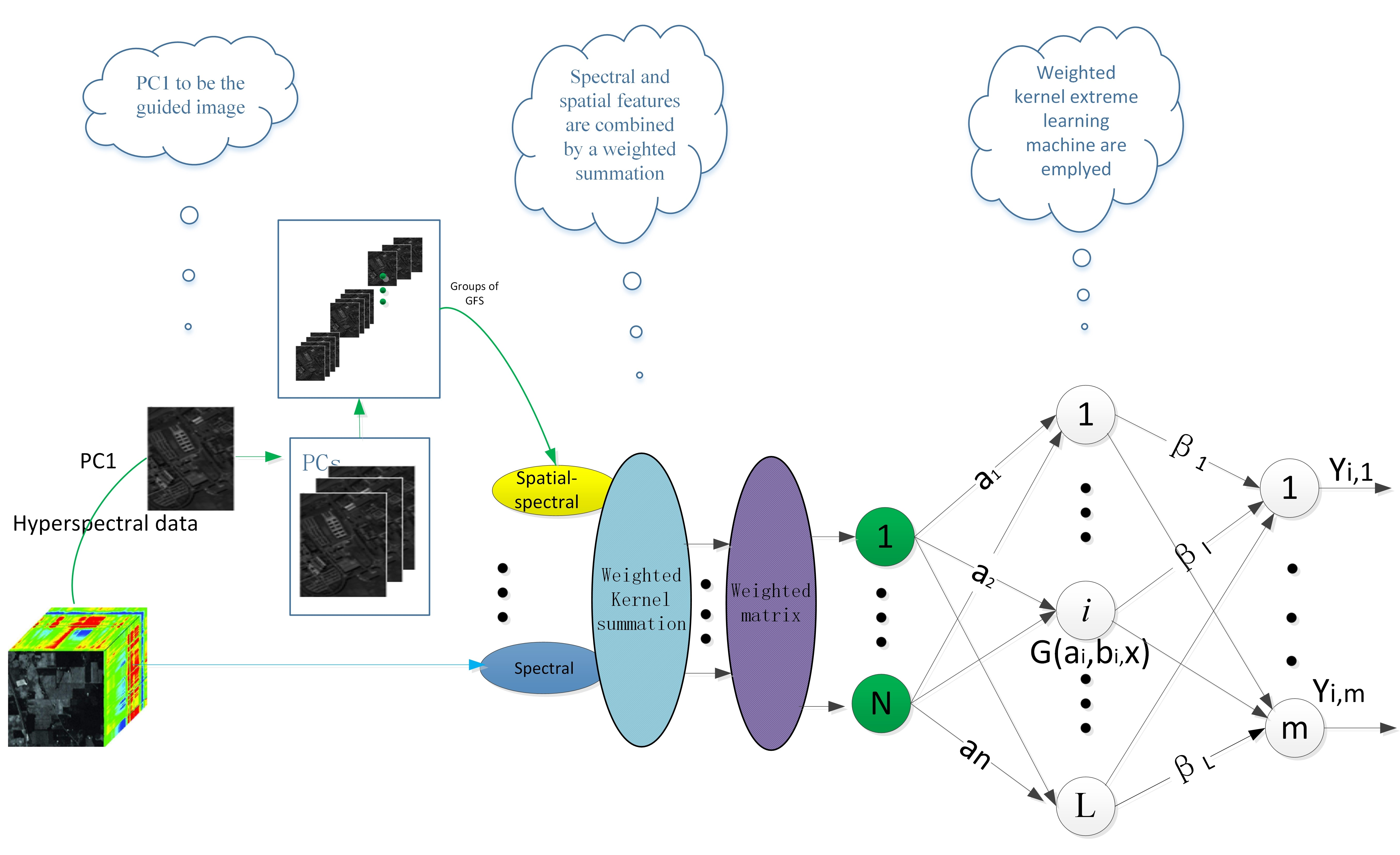
In this section, the proposed dual-weighted kernel extreme learning machine for hyperspectral image classification—termed DW-KELM—is described in detail. The joint spatial–spectral information is employed to investigate the performance of the dual-weighted kernel ELM for hyperspectral imagery classification. Figure 1 shows the procedure of the spatial–spectral dual-weighted kernel ELM-based HSI classification.
For the classification task, principal component analysis (PCA) is applied as a pre-procedure of feature extraction. The PCs that contain 99% of information are preserved. We use the guided filter on PCs that have a group of spatial features.
Given pixel , which is a sample consisting of the spectral characteristics across a continuous range of spectral bands, we denote its spectral and spatial features as and , respectively. The spectral feature vector is the original , which consists of spectral reflection values across all bands. The spatial feature vector is extracted by multiple guided image filtering methods. As the first PC contains most of the useful information, we use it as the guided image in our proposal. The first PC greatly maintains the edge information after these operations, while the other PCs are input images for guided image filtering. Then, we obtained groups of spatial features.
Exploiting the information from the spatial and spectral domains, the kernel method is usually used to perform the spatial–spectral classification. For the kernel method, the original spectral features are used to compute spatial and spectral kernels, which are combined to form kernels.
Once the spatial and spectral features and are constructed, we can compute the spatial kernel and spectral kernel as follows:
Here, we use the Radial Basis Function (RBF)kernel. and are the width of the respective RBF kernels. The Kernel ELM is represented as a weighted kernel summation:
Then, the weighted summation composite kernel is required. The spatial–spectral kernel in Equations (24)–(26) is computed. Then, the features are recalculated using the weighted matrix, , in order to strengthen the impact of the minority class samples. Following this, the dual-weighted kernel ELM model solves:
where the weighted matrix W is the diagonal matrix of the spatial–spectral feature extracted by weighted scheme 2 [41]:
where is the total number belonging to the kth class. is assigned to , that is, the inverse of the minority samples is weighted for the minorities. The golden ratio is used for the majorities.
After the final results are obtained, each test sample is assigned to the highest value in , where , according to the index during the prediction phase:
| Algorithm (Spatial–spectral dual-weighted kernel ELM for HSI classification) |
| Input: HSI data set, r, , L 1. Spectral information is directly extracted from HSI data set. 2. PCA operations are performed and PCs are chosen, according to the quality of information the PCs contain; afterwards, the spatial information is extracted by guided image filtering, according to Equation (23). 3. Kernel weighted summation is formed by spectral and spatial–spectral information, according to Equations (24)–(26). 4. The weighted matrix is acquired, according to Equations (28)–(29). 5. Initiation of the weighted kernel extreme learning machine. 6. Calculation of with Equations (16)–(17). 7. Calculation of the predicted output with Equation (27). 8. Sample is assigned to the highest value, according to Equation (30).End procedure |
3. Experimental Results and Analysis
3.1. Hyperspectral Image Data Sets
The performance of the proposed approach was evaluated using three widely used data sets; namely, Indian Pines, the University of Pavia, and Salinas. The three data sets are publicly available hyperspectral data sets.
3.1.1. Indian Pines
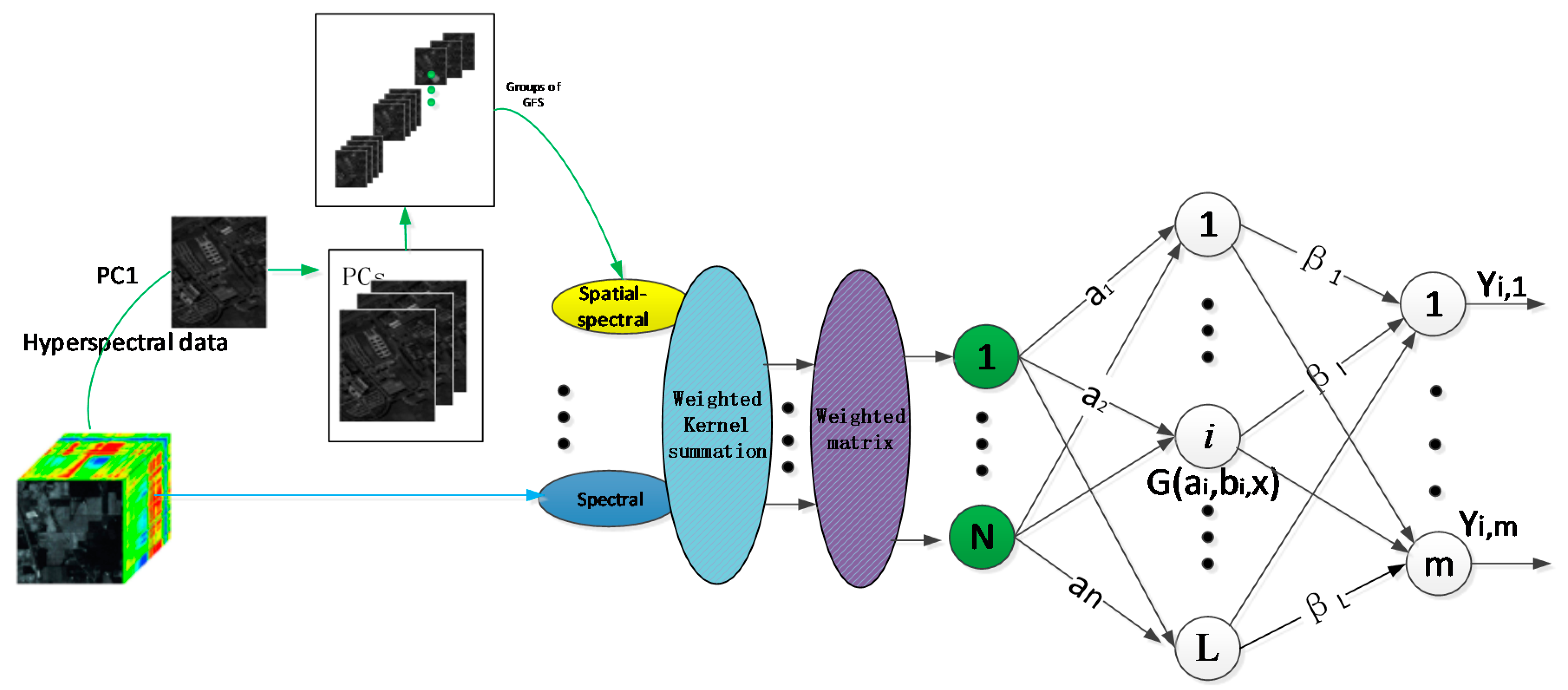
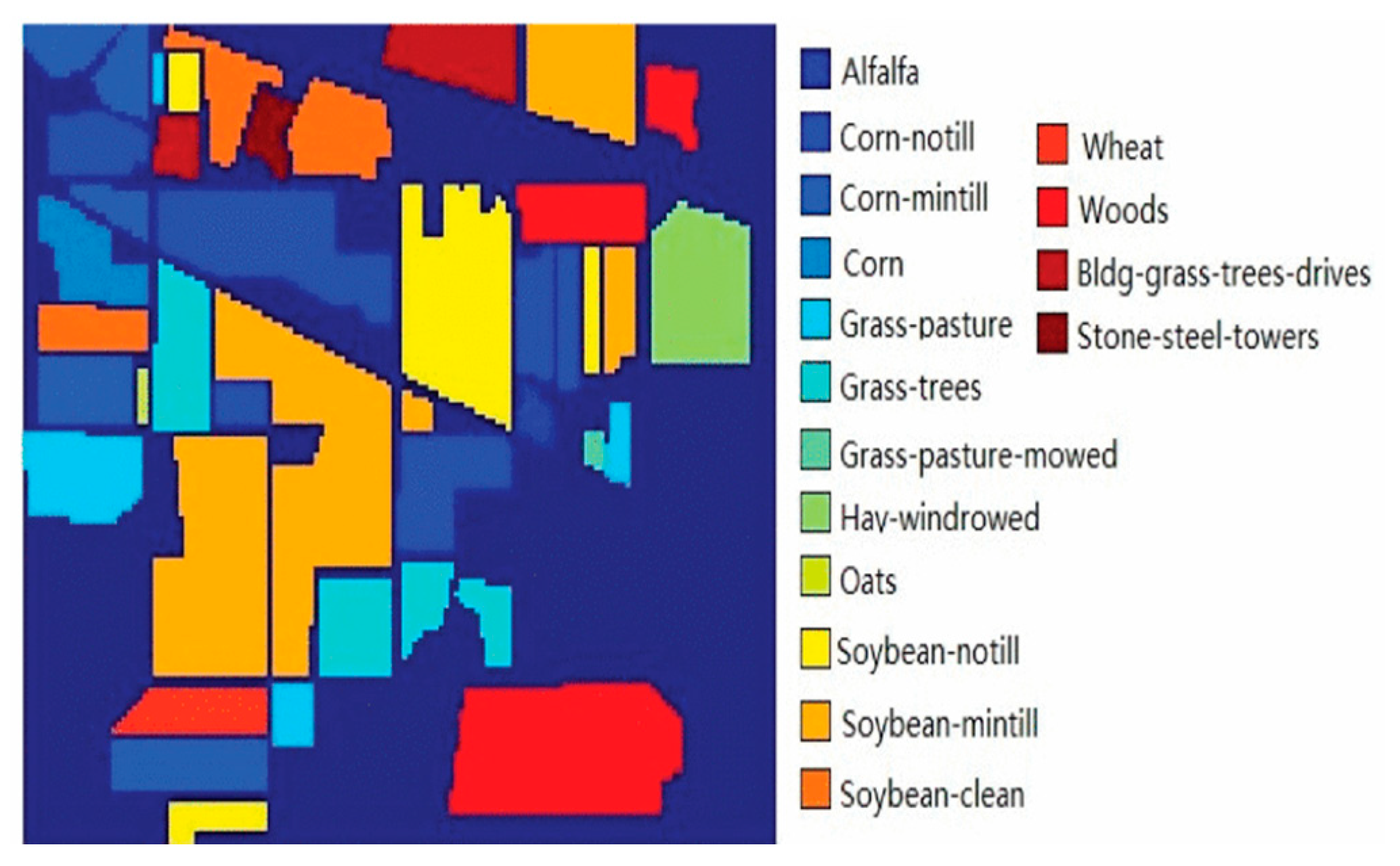
The Indian Pines data set was acquired with the Airborne Visible/Infrared Imaging Spectrometer (AVIRIS) sensor in 1992. The image scene contains 145 × 145 pixels, 220 spectral bands, and a spectral range from 0.4 to 2.5 m, where 20 channels were discarded due to the atmospheric affection. The spatial resolution of the data is 20 m per pixel. The scene contains two-thirds agricultural land and one-third forest or other natural perennial vegetation. Some of the crops present are in early stages of growth, with less than 5% coverage. There are 16 classes and 10,249 labeled samples in the data set in total. The RGB composite image and ground-truth map from the data set are shown in Figure 2.
3.1.2. Pavia University
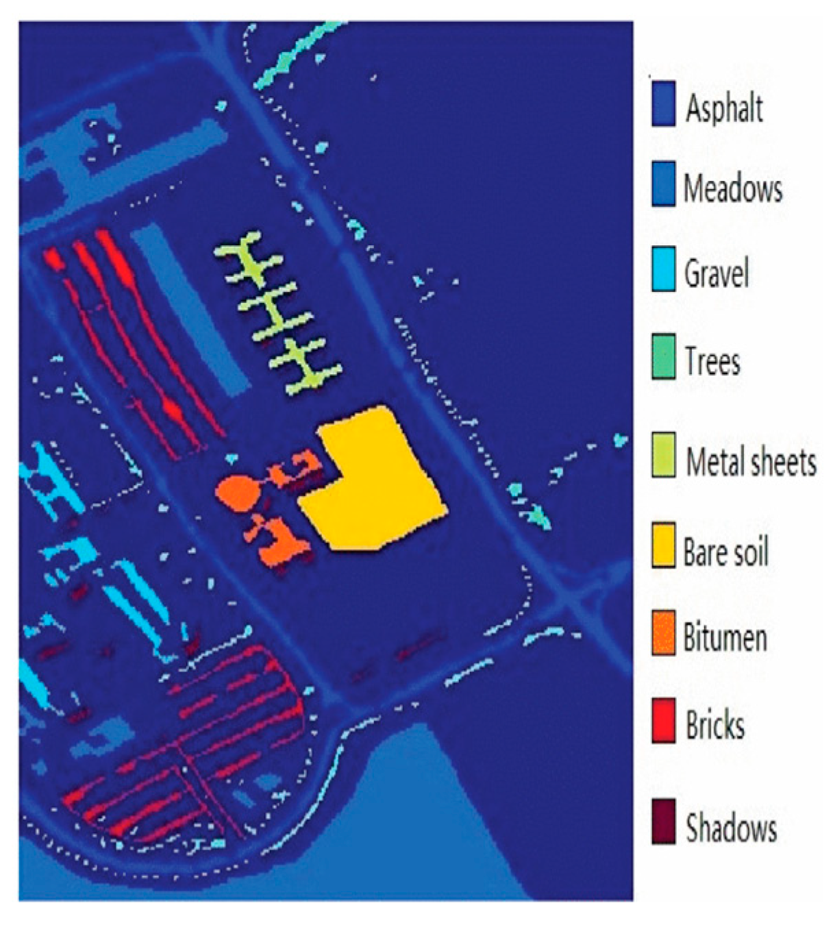
The Pavia University data set was acquired in 2001 using the Reflective Optics System Imaging Spectrometer (ROSIS) instrument over the urban area surrounding the University of Pavia, Italy. This image scene has a size of 610 × 610 pixels. As some of the samples in Pavia University contain no information, we discarded these parts. Thus, the size in our experiment was 610 × 340. The spatial resolution was 1.3 m per pixel. The ROSIS-03 sensor captures 115 spectral bands ranging from 0.43 to 0.86 m. After removing 12 noisy and water-absorption bands, 103 bands were retained. The data contain nine ground-truth classes: asphalt, meadows, gravel, trees, metal sheets, bare soil, bitumen, bricks, and shadows. There was a total of 42,776 labeled samples, The RGB composite image and ground-truth map from the data set are shown in Figure 3.
3.1.3. Salinas
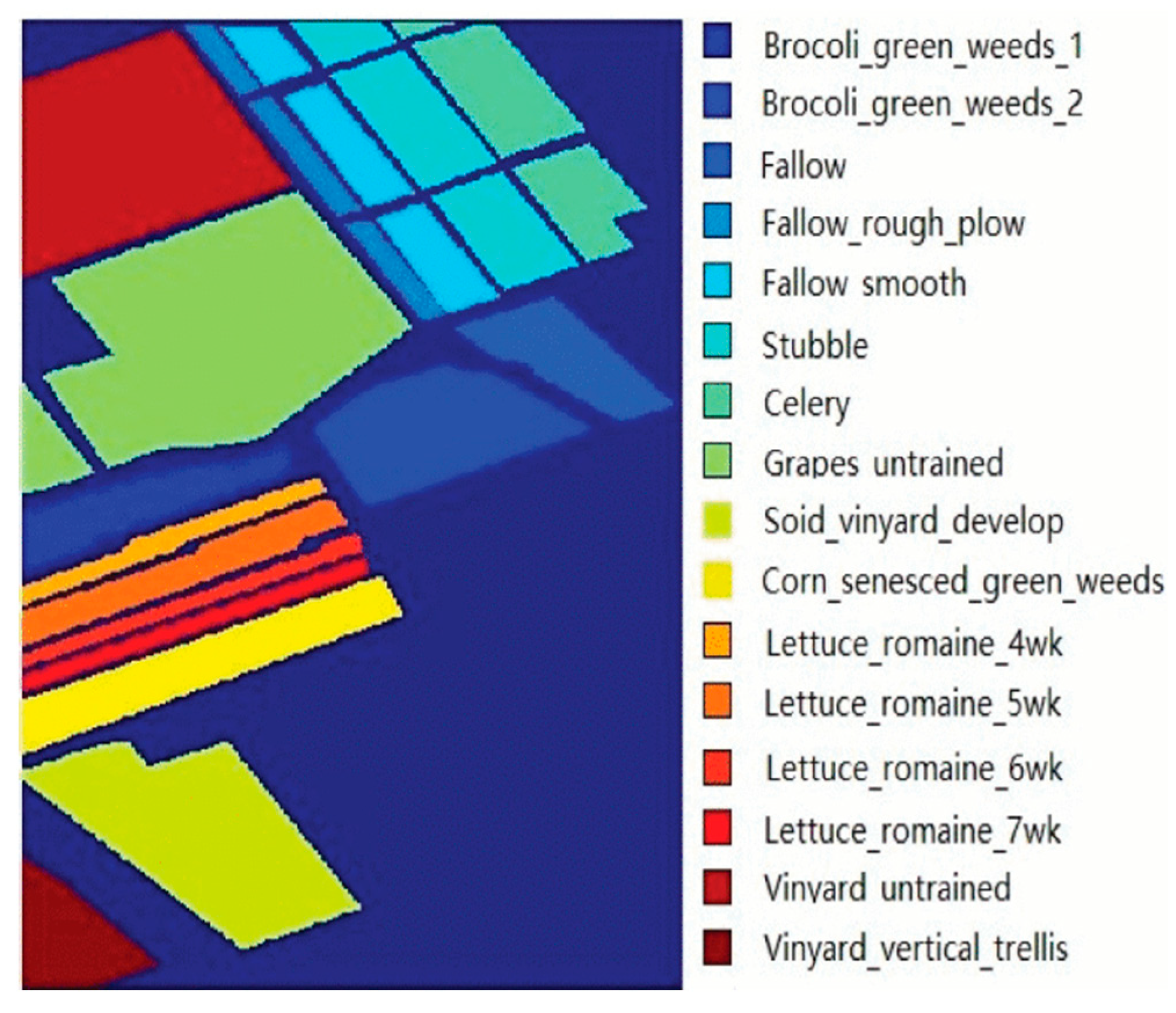
The Salinas data set was acquired using the Airborne Visible/Infrared Imaging Spectrometer (AVIRIS) sensor over Salinas Valley, California, USA. It contains 224 bands and 512 × 217 pixels with 3.7 m spatial resolution per pixel. The data contain 16 ground-truth classes, and 12 noisy and water-absorption bands were removed in the experiment. An image of Salinas is shown in Figure 4.
3.2. Parameter Settings
The classification performance of the different algorithms was assessed on the testing set using the overall accuracy (OA), which is the number of correctly classified testing samples divided by the number of total testing samples; as well as the average accuracy (AA), which represents the average of the classification accuracies for the individual classes; and the kappa (κ) coefficient, which measures the accuracy of classification agreement. The experiments were conducted using MATLAB R2016b on a computer with a 2.8 GHz dual core and 16 GB RAM.
In the pre-processing stage, the principle components (PC) which contained more than 99% information were chosen; PC1 was used as a guided image, the other PCs were used as input images, and the step of the window was .
For the kernel methods, the combination of kernel ELM and coefficient μ was set to 0.95, according to our experience. For all kernel-based algorithms, the RBF kernel was used. The parameter σ varied in the range and C ranged from . The number of hidden nodes for the Indian Pines data set was 500, while those for the University of Pavia and Salinas data sets were 1250 and 650, respectively.
In the general ELM method, the sigmoid function was used and the hidden layer parameters, , were randomly generated based on the uniform distribution in the range of .
3.3. Accuracy of Classification and Analysis
The total number of pixels of Indian Pines available in the reference data was 10,366; however, some classes only had very small labeled samples. To evaluate the performance of different algorithms in this challenging case, we randomly chose 10% of labeled training samples per class. The remaining labeled samples were used for testing. At the same time, for comparison with traditional methods, we also chose 5, 10, 15, 20, 25, and 30 samples as training samples, in order to evaluate the effects of different methods.
The further different algorithms were then compared with seven benchmark algorithms; namely, ELM, kernel ELM (KELM), weighted KELM (WKELM), the spatial feature that uses guided filtering features combined with KELM (SS-KELM), KELM-CK (extreme learning machine e-composite kernel) [21], ASS-H-DELM (average spectral–spatial hierarchical extreme learning machine) [28], and HCKBoost (hybridized composite kernel boosting with extreme learning machines) [27].
3.3.1. Results on the Indian Pines Data Set
The accuracies of the ELM, KELM, WKELM, SS-KELM, KELM-CK, ASS-H-DELM, and HCKBoost measures are provided in Table 1.
From Table 1, it can be observed that the ELM method only required a few seconds for hyperspectral classification application. At the same time, ELM provided the worst results, especially for the classes with limited training samples. The KELM method alleviated this, to some extent, but not significantly. This demonstrates that the kernel used in kernel ELM is more powerful than that which is randomly generated. For the DW-KELM algorithm, when additional spatial information was available, the dual-weighted framework improved the performance of the classifier, while the accuracy dramatically increased. This conclusion can be clearly seen for classes 1, 7, and 9. These three classes contained very similar spectral information, which made the results of classification bad, due to the spectral classifier. Classes 2, 3, 4 are corn subclasses and, thus, had very similar spectral curves; however, the spatial information helped to discriminate the subtle differences and, so, DW-KELM achieved good classification accuracies on corn (more than 95%) and on soybeans (more than 96%). After comparing the cost of time among those methods, it was observed that the ELM method consumes the least amount of time. There are three reasons which explain this phenomenon: Only spectral information was used, the random initial parameters, and the analytic solution for the network. While the same parameter settings were retained, the solution form decides the computation time. It is very common to use the spatial feature as an effective supplement. From the results of classification of classes 1, 7, and 9 for the SS-KELM, KELM-CK, ASS-H-DELM, and HCKBoost algorithms, we can see improvements in both spatial feature use and multiple kernel sides. However, despite the considerable improvement of these methods, the proposed dual-weighted kernel provided more satisfactory results, as the minority class sample was a more important consideration.
Further experiments on the performance with different numbers of labeled training samples per class were conducted, using the three previously introduced data sets. The training set was formed by randomly choosing from 5 to 30 samples, with a step of 5. The remaining samples were used as testing sets. As shown in Table 2, the OA, AA, and κ values were greatly improved with an increase in training numbers. When only spectral information was used, KELM achieved better results than ELM, especially in the condition of extremely small-sized samples. Among the spatial–spectral methods, the proposed DW-KELM showed a significant improvement over the SS-KELM, KELM-CK, ASS-H-DELM, and HCKBoost algorithms. This means that the proposed DW-KELM method is a powerful algorithm for this task, especially for enhancing the performance relating to minority class samples. When the number of training samples was 5 per class, the DW-KELM improved the OA by 4.36%, AA by 4.09%, and κ by 3.50%, while the presence of 30 samples conditions improved the OA by 3.29%, AA by 2.8%, and κ by 3.03%, when compared with HCKBoost on the Indian Pines data set.
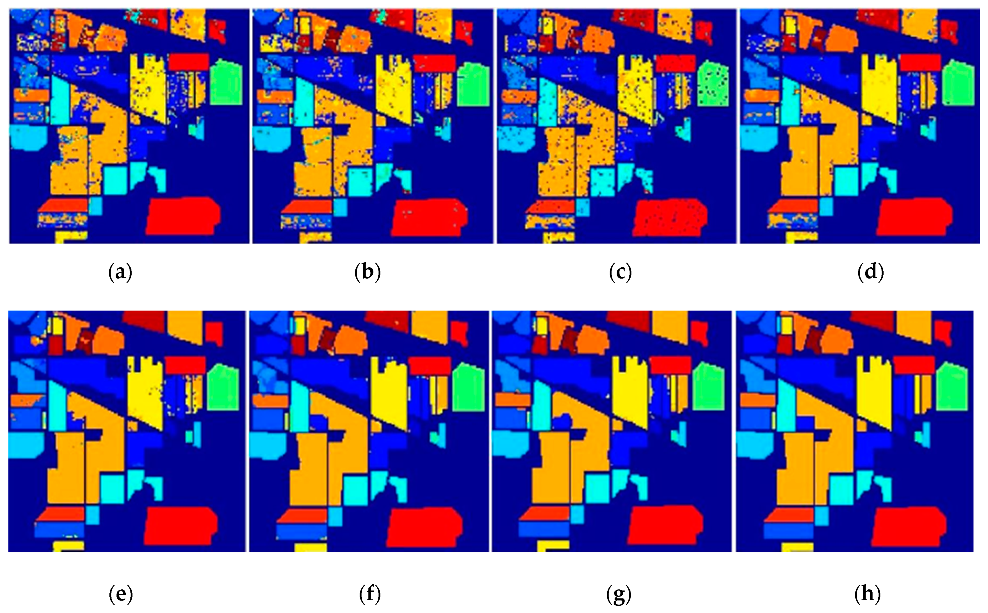
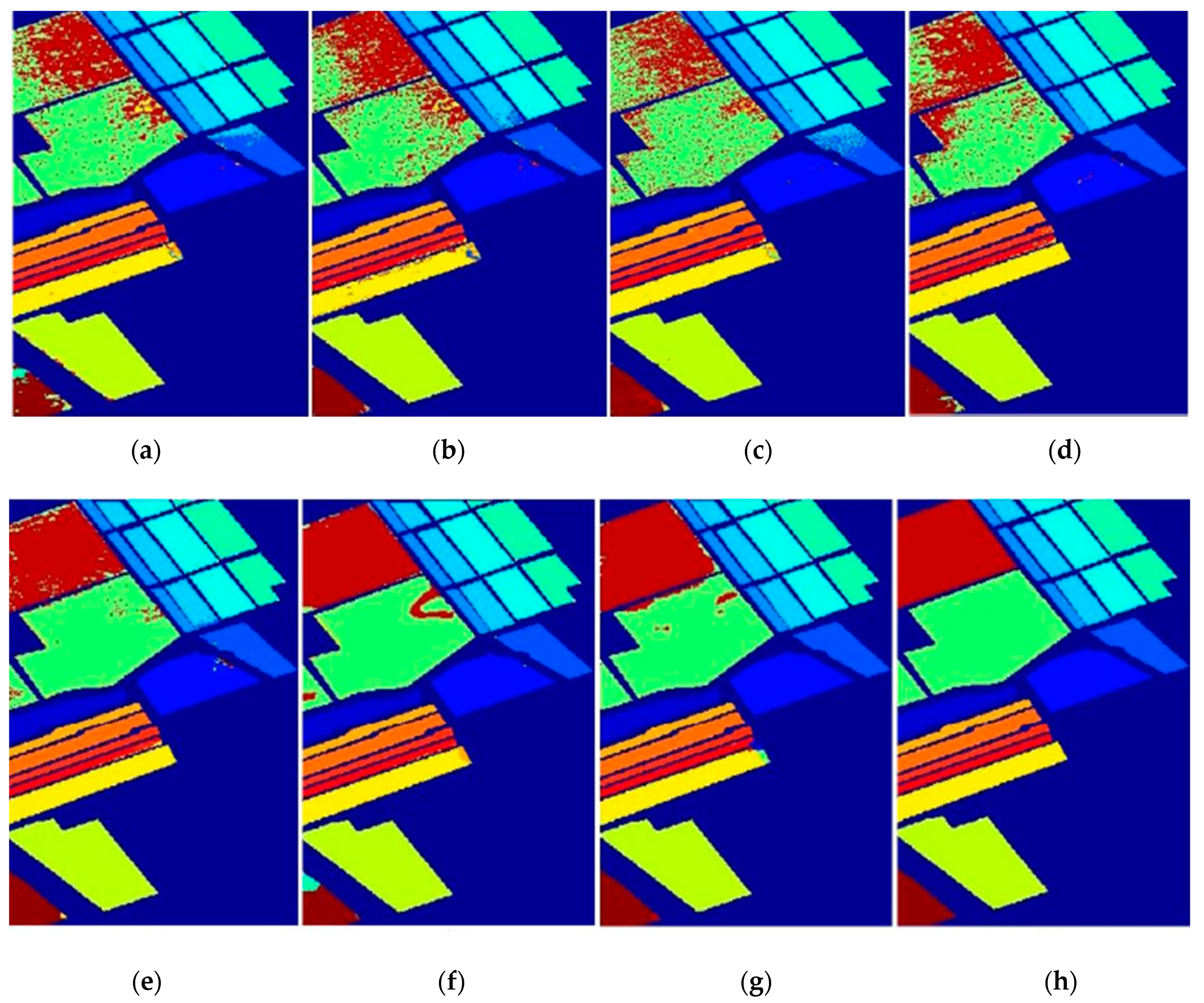
The classification map of the Indian Pines data set is shown in Figure 5. It can be clearly seen that the classification maps of DW-KELM were more coherent in the homogeneous regions, compared with the ELM, KELM, WKELM, SS-KELM, KELM-CK, ASS-H-DELM, and HCKBoost algorithms. In addition, the spatial–spectral methods provided better results than the spectral methods, in terms of consistent classification results with less noise. In particular, in the application of dual-weighted KELM, subtle features and minority samples were considered; this improvement typically arises for classes with similar spectral signatures.
3.3.2. Results on the University of Pavia Image Data Set
The classification results for the University of Pavia images are shown in Figure 6 and the accuracy measures are given in Table 3. The total number of pixels available in the reference data was 414,815. Accordingly, a training set of 10% samples per class were used. Regarding Table 2, the accuracy measures of the proposed ELM-based technique provided equally competitive and even better classification results, when compared to the traditional approaches. The results of the classification of the University of Pavia data set are shown in Figure 7. Figure 8a represents a map of ELM, only using spectral information. The accuracy measures for classification of the University of Pavia image are shown in Table 3. The first columns are the samples that we chose in the experiment.
From Table 3, we can clearly see that, when spatial information and dual-weighted KELM were used, the accuracy of classification was dramatically increased; for instance, for bare soil, from 84.10 to 97.25% and, for bitumen, from 78.93 to 99.90%. There were two main reasons for this: First, the weighted matrix strengthened the importance of class samples, which may be ignored in the presence of many majority class samples; second, TTthe spatial information helped to discriminate samples with similar spectral curves.
When the training samples increased, the OA, AA, and κ values improved, which can be clearly seen from Table 4. When only spectral information was used, ELM provided worse results than KELM. Among the joint spatial and spectral information classification methods, DW-KELM provided the best results. When the number of training samples per class was 30, DW-KELM improved the OA by 3.95%, AA by 2.99%, and κ by2.53% on the University of Pavia image, when compared with the HCKBoost algorithm. It seems that the proposed dual-weighted KELM is not only suitable for data with an imbalanced distribution, but also for balanced data.
3.3.3. Results on the Salinas Image
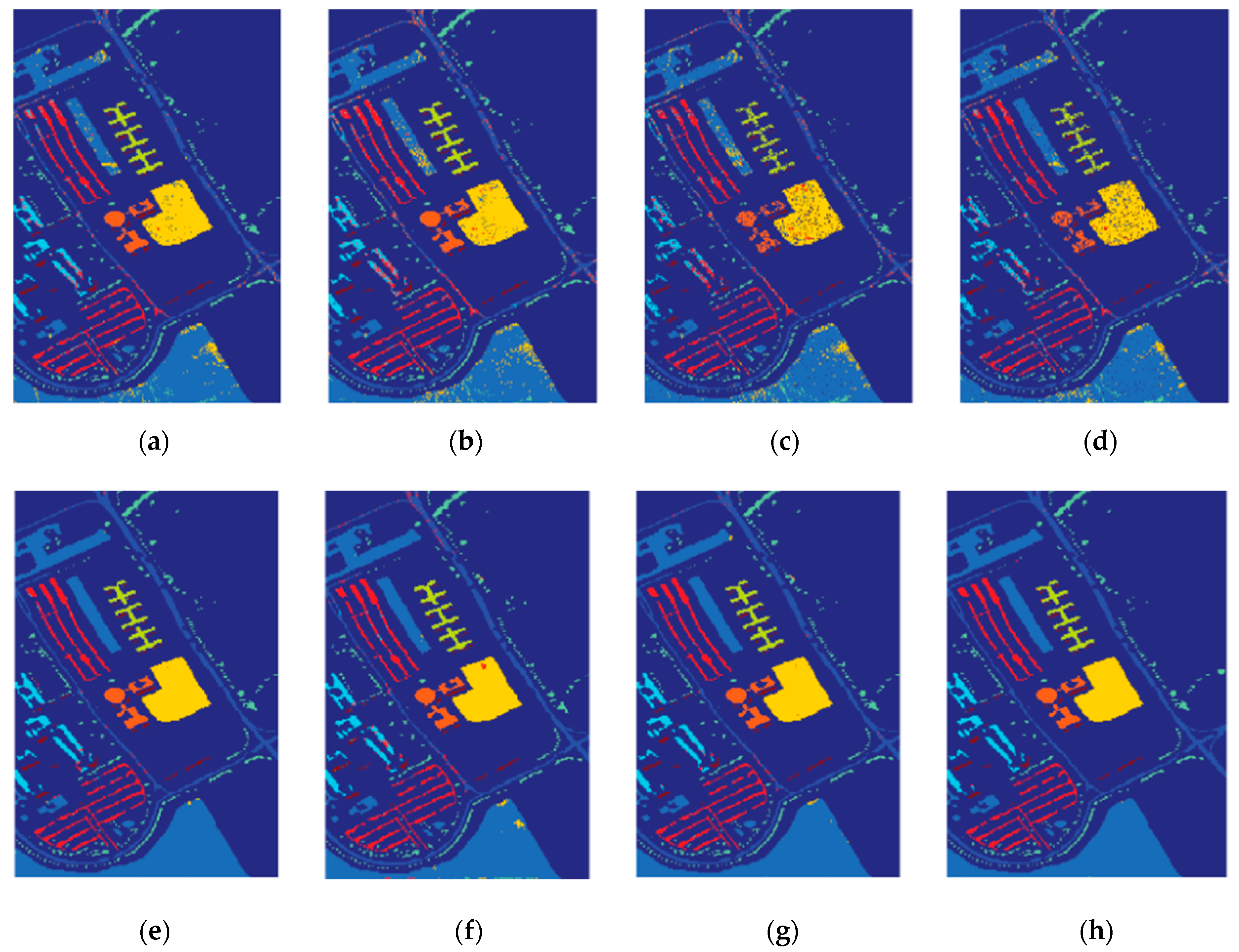
The classification results of different methods for the Salinas image are shown in Figure 8. Similar settings as those in the aforementioned images were used. It can be clearly seen that the classification maps of DW-KELM are more spatially coherent in the large homogeneous region than other methods; further, the results have little noise. The increasing trend of OA, AA, and κ was also the same as for the images of the Indian Pines and Pavia University data sets. Among the other ELM- or KELM-based approaches, DW-KELM improved the OA by 3.72%, AA by 2.32%, and κ by 2.64%, when compared with HCKBoost, on the Salinas image.
From Table 5 and Table 6, we can observe the trend of accuracy change, in all of the experiments, the proposed DW-KELM method provided more accurate results than the other (ELM- or KELM-based) methods. This indicates that the weighted matrix kernel and weighted kernel summations are effective for identifying the subtle differences among similar objects.
3.4. Ablation Study
To evaluate the purpose of our method, the ablation experiments are also carried, which termed as WKELM and SS-KELM respectively. From Table 1 and Table 2, we can clearly see that, without multiple spatial information, the accuracy is not high as those within spatial features methods. At the same time, when the extra weight not assigned to each sample, the accuracy is also not high. Specially, for these samples whose training sample are extremely small, for instance the class 7 and class 9 in the image of Indian Pines, the weight will affect a lot. The same trend happens on the image of Pavia University and the Salinas, we can see these from Table 3, Table 4 and Table 5 and Table 6 respectively.
3.5. G-Mean as a Supplementary Measure for Evaluation
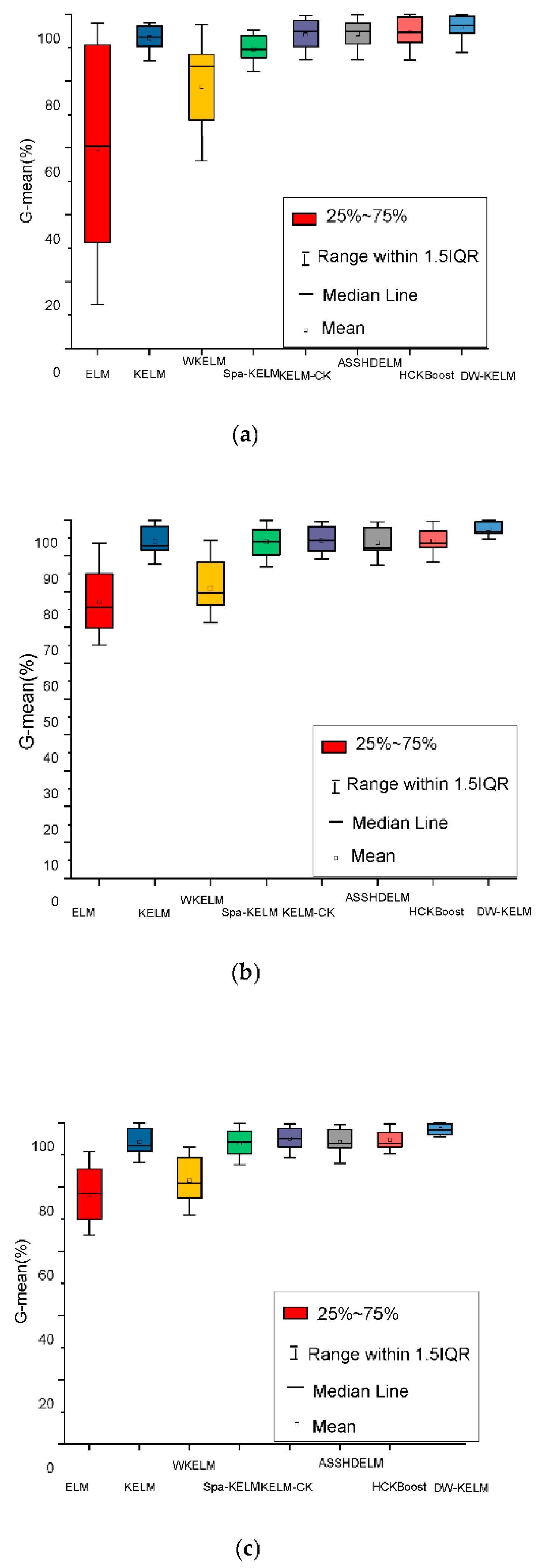
Overall accuracy has been widely used to evaluate the performance of classifiers. In addition, if the samples are imbalanced or distributed, it may not be possible to provide adequate information regarding the generalizability of a classifier; for instance, with a data set which has 10 samples belonging to a negative class and 90 samples belonging to a positive class, if there are 10 misclassified samples, the overall accuracy is equal to 80%, but the G-mean is equal to zero. Thus, we used the G-mean [36] as a supplementary measure to evaluate the performance of the proposed dual-weighted method:
where TP represents the number that correctly classified positive samples and FN is the number of incorrectly classified positive samples.
From the box plot in Figure 8, the results show that the proposed DW-KELM obtained a more concentrated G-mean, especially on the Indian Pines image, due to consideration of the importance of the minority samples. In addition, its interquartile range (IQR) was smaller than those of the other methods.
4. Conclusions
In this paper, a dual-weighted kernel extreme learning machine was proposed, in order to tackle the hyperspectral imagery classification task. It is more effective when using small-sized samples, as the cumulative errors of the minority samples were previously ignored in traditional ELM algorithms. In particular, the weighted matrix W plays an important role in the proposed method; larger weights are assigned to samples from the minority class, thus emphasizing their importance. In addition, as useful supplementary features, the spatial features are fully mined by adding weighted summation. This spatial information contains rich structure features, which help in distinguishing subtle differences in similar classes. The experimental results demonstrated that the proposed DW-KELM method is more accurate than the considered benchmark methods for the classification of hyperspectral imagery.
Author Contributions
X.Y. and Y.F. conceived and designed the experiments; X.Y. implemented the proposed method and analyzed the results of the experiment; Y.G. and Y.J. validated the experiment; S.M. and Y.F. analyzed the results and significantly revised the paper. All authors have read and agreed to the published version of the manuscript.
Funding
This research was funded by the National Natural Science Foundation of China under grant number 61420106007.
Data Availability Statement
The data presented in this study are openly available in the website: http://www.ehu.eus/ccwintco/index.php/Hyperspectral_Remote_Sensing_Scenes.
Acknowledgments
The authors thank the Editor-in-Chief, the Associate Editor, and the anonymous reviewers for their suggestions and insightful comments on this paper.
Conflicts of Interest
The authors declare no conflict of interest.
References
- Camps-Valls, G.; Tuia, D.; Bruzzone, L.; Benediktsson, J.A. Advances in Hyperspectral Image Classification: Earth Monitoring with Statistical Learning Methods. IEEE Signal Process. Mag. 2014, 31, 45–54. [Google Scholar] [CrossRef] [Green Version]
- Gualtieri, J.A.; Cromp, R.F. Support vector machines for hyperspectral remote sensing classification. Proc. SPIE Workshop Adv. Comput. Assist. Recognit. 1998, 3584, 221–232. [Google Scholar]
- Campsvalls, G.; Gomezchova, L.; Munozmari, J.; Vilafrances, J.; Calpemaravilla, J. Composite kernels for hyperspectral image classification. IEEE Geosci. Remote Sens. Lett. 2006, 3, 93–97. [Google Scholar] [CrossRef]
- Fauvel, M.; Chanussot, J.; Benediktsson, J.A. Evaluation of kernels for multiclass classification of hyperspectral remote sensing data. In Proceedings of the 2006 IEEE International Conference on Acoustics Speech and Signal Processing Proceedings, Toulouse, France, 14–19 May 2006; p. II. [Google Scholar] [CrossRef]
- Fauvel, M.; Arbelot, B.; Benediktsson, J.A.; Sheeren, D.; Chanussot, J. Detection of Hedges in a Rural Landscape Using a Local Orientation Feature: From Linear Opening to Path Opening. IEEE J. Sel. Top. Appl. Earth Obs. Remote Sens. 2013, 6, 15–26. [Google Scholar] [CrossRef]
- Valero, S.; Chanussot, J.; Benediktsson, J.A.; Talbot, H.; Waske, B. Advanced directional mathematical morphology of the detection of the road network in very high resolution remote sensing images. Pattern Recognit. Lett. 2010, 31, 1120–1127. [Google Scholar] [CrossRef] [Green Version]
- Fang, L.; Li, S.; Duan, W.; Ren, J.; Benediktsson, J.A. Classification of Hyperspectral Images by Exploiting Spectral-Spatial Information of Super pixel via Multiple Kernels. IEEE Trans. Geosci. Remote Sens. 2015, 53, 6663–6674. [Google Scholar] [CrossRef] [Green Version]
- Wu, H.; Prasad, S. Semi-Supervised Deep Learning Using Pseudo Labels for Hyperspectral Image Classification. IEEE Trans. Image Process. 2018, 27, 1259–1270. [Google Scholar] [CrossRef] [PubMed]
- Pan, B.; Xu, X.; Shi, Z.; Zhang, N.; Luo, H.; Lan, X. DSSNet: A Simple Dilated Semantic Segmentation Network for Hyperspectral Imagery Classification. IEEE Geosci. Remote Sens. Lett. 2020, 17, 1968–1972. [Google Scholar] [CrossRef]
- Pan, B.; Shi, Z.; Xu, X. R-VCANet: A New Deep-Learning-Based Hyperspectral Image Classification Method. IEEE J. Sel. Top. Appl. Earth Obs. Remote Sens. 2017, 10, 1975–1986. [Google Scholar] [CrossRef]
- Mei, S.; Ji, J.; Geng, Y.; Zhang, Z.; Li, X.; Du, Q. Unsupervised Spatial–Spectral Feature Learning by 3D Convolutional Autoencoder for Hyperspectral Classification. IEEE Trans. Geosci. Remote Sens. 2019, 57, 6808–6820. [Google Scholar] [CrossRef]
- Peng, J.; Sun, W.; Du, Q. Self-Paced Joint Sparse Representation for the Classification of Hyperspectral Images. IEEE Trans. Geosci. Remote Sens. 2019, 57, 1183–1194. [Google Scholar] [CrossRef]
- Peng, J.; Li, L.; Tang, Y.Y. Maximum Likelihood Estimation-Based Joint Sparse Representation for the Classification of Hyperspectral Remote Sensing Images. IEEE Trans. Neural Netw. Learn. Syst. 2019, 30, 1790–1802. [Google Scholar] [CrossRef] [PubMed]
- Yuan, Y.; Lin, J.; Wang, Q. Hyperspectral Image Classification via Multitask Joint Sparse Representation and Stepwise MRF Optimization. IEEE Trans. Cybern. 2016, 46, 2966–2977. [Google Scholar] [CrossRef] [PubMed]
- Gu, Y.; Liu, T.; Jia, X.; Benediktsson, J.A.; Chanussot, J. Nonlinear Multiple Kernel Learning with Multiple-Structure-Element Extended Morphological Profiles for Hyperspectral Image Classification. IEEE Trans. Geosci. Remote Sens. 2016, 54, 3235–3247. [Google Scholar] [CrossRef]
- Li, J.; Marpu, P.R.; Plaza, A.; Bioucas-Dias, J.M.; Benediktsson, J.A. Generalized Composite Kernel Framework for Hyperspectral Image Classification. IEEE Trans. Geosci. Remote Sens. 2013, 51, 4816–4829. [Google Scholar] [CrossRef]
- Li, W.; Prasad, S.; Fowler, J.E. Decision Fusion in Kernel-Induced Spaces for Hyperspectral Image Classification. IEEE Trans. Geosci. Remote Sens. 2014, 52, 3399–3411. [Google Scholar] [CrossRef] [Green Version]
- Fang, L.; He, N.; Li, S.; Ghamisi, P.; Benediktsson, J.A. Extinction Profiles Fusion for Hyperspectral Images Classification. IEEE Trans. Geosci. Remote Sens. 2017, 56, 1803–1815. [Google Scholar] [CrossRef]
- Huang, G.B.; Zhou, H.; Ding, X.; Zhang, R. Extreme Learning Machine for Regression and Multiclass Classification. IEEE Trans. Syst. Man Cybern. Part B 2012, 42, 513–529. [Google Scholar] [CrossRef] [Green Version]
- Pal, M.; Maxwell, A.E.; Warner, T.A. Kernel-based extreme learning machine for remote sensing image classification. Remote Sens. Lett. 2013, 4, 853–862. [Google Scholar] [CrossRef]
- Zhou, Y.; Peng, J.; Chen, C.L.P. Extreme Learning Machine with Composite Kernels for Hyperspectral Image Classification. IEEE J. Sel. Top. Appl. Earth Obs. Remote Sens. 2015, 8, 2351–2360. [Google Scholar] [CrossRef]
- Chen, C.; Li, W.; Su, H.; Liu, K. Spectral-Spatial Classification of Hyperspectral Image Based on Kernel Extreme Learning Machine. Remote Sens. 2014, 6, 5795–5814. [Google Scholar] [CrossRef] [Green Version]
- Argüello, F.; Heras, D.B. ELM-based spectral–spatial classification of hyperspectral images using extended morphological profiles and composite feature mappings. Int. J. Remote Sens. 2015, 36, 645–664. [Google Scholar] [CrossRef]
- Jiang, M.; Cao, F.; Lu, Y. Extreme Learning Machine with Enhanced Composite Feature for Spectral-Spatial Hyperspectral Image Classification. IEEE Access 2018, 6, 22645–22654. [Google Scholar] [CrossRef]
- Cao, F.; Yang, Z.; Ren, J.; Ling, B.W.-K.; Zhao, H.; Sun, M.; Benediktsson, J.A. Sparse Representation-Based Augmented Multinomial Logistic Extreme Learning Machine with Weighted Composite Features for Spectral–Spatial Classification of Hyperspectral Images. IEEE Trans. Geosci. Remote Sens. 2018, 56, 6263–6279. [Google Scholar] [CrossRef] [Green Version]
- Li, J.; Xi, B.; Du, Q.; Song, R.; Li, Y.; Ren, G. Deep Kernel Extreme-Learning Machine for the Spectral–Spatial Classification of Hyperspectral Imagery. Remote Sens. 2018, 10, 2036. [Google Scholar] [CrossRef] [Green Version]
- Ergul, U.; Bilgin, G. HCKBoost: Hybridized composite kernel boosting with extreme learning machines for hyperspectral image classification. Neurocomputing 2019, 334, 100–113. [Google Scholar] [CrossRef]
- Le, B.T.; Ha, T.T.L. Hyperspectral image classification based on average spectral-spatial features and improved hierarchical-ELM. Infrared Phys. Technol. 2019, 102, 103013. [Google Scholar] [CrossRef]
- Lv, F.; Han, M. Hyperspectral image classification based on multiple reduced kernel extreme learning machine. Int. J. Mach. Learn. Cybern. 2019, 10, 3397–3405. [Google Scholar] [CrossRef]
- Marpu, P.R.; Pedergnana, M.; Mura, M.D.; Benediktsson, J.A.; Bruzzone, L. Automatic Generation of Standard Deviation Attribute Profiles for Spectral–Spatial Classification of Remote Sensing Data. IEEE Geosci. Remote Sens. Lett. 2013, 10, 293–297. [Google Scholar] [CrossRef]
- Su, H.; Cai, Y.; Du, Q. Firefly-Algorithm-Inspired Framework with Band Selection and Extreme Learning Machine for Hyperspectral Image Classification. IEEE J. Sel. Top. Appl. Earth Obs. Remote Sens. 2017, 10, 309–320. [Google Scholar] [CrossRef]
- Su, H.; Tian, S.; Cai, Y.; Sheng, Y.; Chen, C.; Najafian, M. Optimized extreme learning machine for urban land cover classification using hyperspectral imagery. Front. Earth Sci. 2017, 11, 765–773. [Google Scholar] [CrossRef]
- Li, J.; Du, Q.; Li, W.; Li, Y. Optimizing extreme learning machine for hyperspectral image classification. J. Appl. Remote Sens. 2015, 9, 97296. [Google Scholar] [CrossRef]
- Lv, F.; Han, M.; Qiu, T. Remote Sensing Image Classification Based on Ensemble Extreme Learning Machine with Stacked Autoencoder. IEEE Access 2017, 5, 9021–9031. [Google Scholar] [CrossRef]
- He, K.; Sun, J.; Tang, X. Guided Image Filtering. IEEE Trans. Pattern Anal. Mach. Intell. 2013, 35, 1397–1409. [Google Scholar] [CrossRef]
- Pan, B.; Shi, Z.; Xu, X. Hierarchical Guidance Filtering-Based Ensemble Classification for Hyperspectral Images. IEEE Trans. Geosci. Remote Sens. 2017, 55, 4177–4189. [Google Scholar] [CrossRef]
- Guo, Y.; Yin, X.; Zhao, X.; Yang, D.; Bai, Y. Hyperspectral image classification with SVM and guided filter. EURASIP J. Wirel. Commun. Netw. 2019, 2019, 56. [Google Scholar] [CrossRef]
- Wang, Z.; Hu, H.; Zhang, L.; Xue, J.-H. Discriminatively guided filtering (DGF) for hyperspectral image classification. Neurocomputing 2018, 275, 1981–1987. [Google Scholar] [CrossRef] [Green Version]
- Li, Z.; Zheng, J.; Zhu, Z.; Yao, W.; Wu, S. Weighted Guided Image Filtering. IEEE Trans. Image Process. 2015, 24, 120–129. [Google Scholar] [CrossRef]
- Fletcher, R. Practical Methods of Optimization: Constrained Optimization; Wiley: New York, NY, USA, 1981; Volume 2, pp. 143–144. [Google Scholar]
- Zong, W.; Huang, G.-B.; Chen, Y. Weighted extreme learning machine for imbalance learning. Neurocomputing 2013, 101, 229–242. [Google Scholar] [CrossRef]
- Raghuwanshi, B.S.; Shukla, S. Class imbalance learning using UnderBagging based kernelized extreme learning machine. Neurocomputing 2019, 329, 172–187. [Google Scholar] [CrossRef]
Figure 1.
Flowchart of the proposed dual-weight kernel extreme learning method.

Figure 2.
Ground truth of the Indian Pines data set.

Figure 3.
Ground truth of the Pavia University data set.

Figure 4.
Ground truth map of the Salinas data set.

Figure 5.
Classification map of the Indian Pines data set with 30 samples: (a) ELM, (b) KELM, (c) WKELM, (d) SS-KELM, (e) KELM-CK, (f) ASS-H-DELM, (g) HCKBoost, and (h) DW-KELM.
Figure 5.
Classification map of the Indian Pines data set with 30 samples: (a) ELM, (b) KELM, (c) WKELM, (d) SS-KELM, (e) KELM-CK, (f) ASS-H-DELM, (g) HCKBoost, and (h) DW-KELM.

Figure 6.
Classification map of the University of Pavia: (a) ELM, (b) KELM, (c) WKELM, (d) SS-KELM, (e) KELM-CK, (f) ASS-H-DELM, (g) HCKBoost, and (h) DW-KELM.
Figure 6.
Classification map of the University of Pavia: (a) ELM, (b) KELM, (c) WKELM, (d) SS-KELM, (e) KELM-CK, (f) ASS-H-DELM, (g) HCKBoost, and (h) DW-KELM.

Figure 7.
Classification map of the Salinas data set with 30 samples: (a) ELM, (b) KELM, (c) WKELM, (d) SS-KELM, (e) KELM-CK, (f) ASS-H-DELM, (g) HCKBoost, (h) and DW-KELM.
Figure 7.
Classification map of the Salinas data set with 30 samples: (a) ELM, (b) KELM, (c) WKELM, (d) SS-KELM, (e) KELM-CK, (f) ASS-H-DELM, (g) HCKBoost, (h) and DW-KELM.

Figure 8.
G-mean (%) on the (a) Indian Pines, (b) Pavia University, and (c) Salinas images.


Table 1.
Overall accuracy (OA), average accuracy (AA), and kappa (%) obtained by different approaches on the Indian Pines data set.
Table 1.
Overall accuracy (OA), average accuracy (AA), and kappa (%) obtained by different approaches on the Indian Pines data set.
| Class No. | Train/Test | ELM | KELM | WKELM | SS-KELM | KELM-CK | ASS-H-DELM | HCKBoost | DW-KELM |
|---|---|---|---|---|---|---|---|---|---|
| 1 | 5/41 | 43.14 | 81.65 | 86.75 | 84.55 | 87.92 | 86.50 | 87.23 | 91.42 |
| 2 | 143/1285 | 70.51 | 73.03 | 74.19 | 90.23 | 90.65 | 89.80 | 89.88 | 88.98 |
| 3 | 883/747 | 45.61 | 73.25 | 76.70 | 93.86 | 95.10 | 95.12 | 94.16 | 96.29 |
| 4 | 24/213 | 42.24 | 62.16 | 68.75 | 66.38 | 92.86 | 92.66 | 93.52 | 94.36 |
| 5 | 50/433 | 85.96 | 88.53 | 89.97 | 94.15 | 94.63 | 95.35 | 94.27 | 97.14 |
| 6 | 75/655 | 92.16 | 92.61 | 93.58 | 94.70 | 95.85 | 95.40 | 99.65 | 99.62 |
| 7 | 3/25 | 20.26 | 66.58 | 72.13 | 69.22 | 97.05 | 94.68 | 95.10 | 96.96 |
| 8 | 49/429 | 96.64 | 96.08 | 97.08 | 97.35 | 99.50 | 99.45 | 99.43 | 99.98 |
| 9 | 2/18 | 23.30 | 63.21 | 73.71 | 68.35 | 99.45 | 99.13 | 100 | 99.85 |
| 10 | 97/875 | 50.38 | 79.91 | 83.56 | 94.27 | 90.01 | 95.60 | 96.31 | 93.30 |
| 11 | 247/2208 | 79.82 | 86.35 | 88.71 | 95.12 | 95.25 | 94.48 | 96.55 | 98.34 |
| 12 | 62/531 | 45.18 | 82.24 | 84.62 | 85.35 | 87.62 | 88.26 | 89.34 | 95.61 |
| 13 | 22/183 | 97.26 | 99.01 | 99.45 | 99.13 | 99.03 | 99.10 | 99.25 | 99.38 |
| 14 | 130/1135 | 97.27 | 97.44 | 97.75 | 98.35 | 99.67 | 99.85 | 99.30 | 99.80 |
| 15 | 38/348 | 40.17 | 72.58 | 76.29 | 75.20 | 91.28 | 92.68 | 93.29 | 96.75 |
| 16 | 10/83 | 46.20 | 86.23 | 87.13 | 87.25 | 86.53 | 88.59 | 86.36 | 94.69 |
| OA | 63.52 | 84.45 | 88.25 | 94.55 | 94.28 | 94.30 | 94.55 | 98.25 | |
| std | 1.05 | 1.29 | 0.95 | 0.95 | 0.69 | 0.88 | 0.95 | 0.95 | |
| AA | 56.06 | 81.57 | 84.25 | 90.28 | 93.18 | 93.16 | 93.27 | 98.27 | |
| std | 1.83 | 2.26 | 1.41 | 1.56 | 1.72 | 1.16 | 0.63 | 0.99 | |
| κ | 65.37 | 80.73 | 84.52 | 84.52 | 93.16 | 93.22 | 92.19 | 94.25 | |
| std | 1.25 | 2.44 | 2.30 | 2.30 | 0.72 | 0.75 | 1.16 | 0.86 | |
| Time(s) | 0.35 | 3.65 | 5.41 | 47.56 | 43.67 | 135.25 | 322.45 | 96.26 | |
| std | 0.03 | 0.38 | 0.85 | 1.08 | 0.68 | 0.65 | 1.05 | 0.58 | |
Table 2.
OA, AA, and kappa (%) obtained with different training numbers of labeled samples per class on the Indian Pines data set.
Table 2.
OA, AA, and kappa (%) obtained with different training numbers of labeled samples per class on the Indian Pines data set.
| Training Numbers | Assessments | ELM | KELM | WKELM | SS-KELM | KELM-CK | ASS-H-DELM | HCKBoost | DW-KELM |
|---|---|---|---|---|---|---|---|---|---|
| 5 | OA | 42.61 | 48.33 | 51.25 | 65.23 | 64.80 | 65.42 | 66.14 | 70.50 |
| std | 1.23 | 2.88 | 2.37 | 2.55 | 0.85 | 1.28 | 0.55 | 3.22 | |
| AA | 53.01 | 61.25 | 64.75 | 74.58 | 76.25 | 77.80 | 77.45 | 81.91 | |
| std | 2.17 | 1.87 | 1.95 | 1.29 | 1.46 | 0.66 | 1.17 | 1.83 | |
| κ | 36.45 | 42.67 | 44.56 | 62.06 | 58.95 | 64.35 | 64.62 | 68.12 | |
| std | 2.93 | 3.12 | 2.23 | 2.12 | 0.67 | 1.25 | 1.25 | 3.35 | |
| 10 | OA | 55.22 | 62.22 | 65.26 | 73.52 | 74.85 | 76.95 | 77.25 | 80.84 |
| std | 2.15 | 2.17 | 1.89 | 2.27 | 1.45 | 1.23 | 0.87 | 4.01 | |
| AA | 68.58 | 73.50 | 75.53 | 80.35 | 79.12 | 90.23 | 91.13 | 92.26 | |
| std | 2.85 | 1.98 | 1.66 | 1.35 | 2.26 | 0.68 | 1.65 | 2.99 | |
| κ | 50.61 | 58.27 | 62.75 | 65.16 | 72.35 | 70.15 | 73.52 | 78.53 | |
| std | 2.21 | 2.31 | 1.99 | 2.54 | 0.75 | 0.95 | 0.95 | 4.59 | |
| 15 | OA | 62.59 | 68.12 | 71.19 | 73.56 | 79.56 | 82.12 | 83.14 | 87.28 |
| std | 1.55 | 2.21 | 2.09 | 2.113 | 1.46 | 1.55 | 1.54 | 2.67 | |
| AA | 74.62 | 78.29 | 78.29 | 83.59 | 88.23 | 89.52 | 90.25 | 94.26 | |
| std | 1.75 | 1.25 | 1.25 | 1.86 | 1.68 | 0.68 | 1.44 | 1.35 | |
| κ | 60.45 | 63.82 | 65.28 | 76.18 | 79.12 | 81.65 | 82.06 | 84.72 | |
| std | 1.22 | 2.23 | 1.85 | 2.53 | 1.88 | 1.56 | 0.92 | 2.66 | |
| 20 | OA | 68.10 | 69.26 | 72.35 | 81.53 | 87.85 | 84.56 | 85.16 | 89.91 |
| std | 1.05 | 1.31 | 1.56 | 1.68 | 1.72 | 0.68 | 1.18 | 1.23 | |
| AA | 78.29 | 80.20 | 83.69 | 88.53 | 94.56 | 93.13 | 94.25 | 95.59 | |
| std | 1.78 | 2.44 | 1.49 | 2.32 | 0.85 | 1.35 | 0.79 | 2.28 | |
| κ | 64.87 | 67.65 | 70.65 | 83.12 | 86.89 | 85.65 | 86.16 | 89.86 | |
| std | 0.98 | 3.10 | 2.69 | 2.29 | 1.27 | 0.58 | 1.59 | 2.55 | |
| 25 | OA | 69.42 | 71.21 | 73.25 | 83.23 | 87.85 | 88.45 | 89.26 | 93.06 |
| std | 3.31 | 2.21 | 2.47 | 1.35 | 1.72 | 0.65 | 1.75 | 2.28 | |
| AA | 79.35 | 82.20 | 84.55 | 89.55 | 94.56 | 94.18 | 95.25 | 97.23 | |
| std | 1.52 | 2.41 | 1.85 | 1.56 | 0.85 | 0.65 | 1.97 | 1.12 | |
| κ | 65.29 | 67.65 | 69.96 | 85.02 | 86.89 | 88.12 | 89.92 | 92.51 | |
| std | 1.25 | 3.10 | 2.83 | 2.14 | 1.27 | 0.86 | 0.76 | 2.90 | |
| 30 | OA | 71.21 | 72.59 | 75.66 | 88.56 | 93.52 | 94.15 | 94.59 | 97.88 |
| std | 1.72 | 2.62 | 1.82 | 0.56 | 0.55 | 0.73 | 1.14 | 1.21 | |
| AA | 80.55 | 82.90 | 84.59 | 90.42 | 96.51 | 96.12 | 96.35 | 99.15 | |
| std | 0.88 | 1.82 | 1.16 | 0.73 | 0.38 | 0.75 | 0.66 | 0.96 | |
| κ | 67.37 | 69.82 | 72.59 | 87.05 | 90.68 | 91.65 | 92.39 | 95.42 | |
| std | 2.21 | 1.75 | 1.69 | 1.35 | 0.75 | 0.64 | 1.36 | 0.87 |
Table 3.
OA, AA, and kappa (%) obtained by different approaches on the Pavia University data set for different classes.
Table 3.
OA, AA, and kappa (%) obtained by different approaches on the Pavia University data set for different classes.
| Class | Train/test | ELM | KELM | WKELM | SS-KELM | ASS-H-DELM | CK-KELM | HCKBoost | DW-KELM |
|---|---|---|---|---|---|---|---|---|---|
| 1 | 64/6599 | 72.56 | 77.15 | 80.28 | 91.82 | 92.88 | 92.60 | 95.15 | 100 |
| 2 | 184/18465 | 74.35 | 75.28 | 78.46 | 93.59 | 92.19 | 95.55 | 93.29 | 98.88 |
| 3 | 20/2079 | 66.19 | 67.13 | 78.37 | 86.551 | 86.99 | 86.28 | 90.03 | 94.29 |
| 4 | 28/3026 | 67.45 | 68.27 | 72.18 | 93.65 | 92.59 | 92.09 | 93.50 | 95.47 |
| 5 | 11/1134 | 70.23 | 74.52 | 77.28 | 97.59 | 95.35 | 97.46 | 97.86 | 98.27 |
| 6 | 48/4981 | 79.53 | 82.33 | 84.19 | 94.90 | 94.53 | 95.58 | 94.91 | 98.36 |
| 7 | 11/1319 | 76.58 | 78.65 | 82.34 | 95.29 | 97.28 | 95.36 | 95.28 | 97.85 |
| 8 | 34/3648 | 75.86 | 79.21 | 80.25 | 86.90 | 89.33 | 87.89 | 88.45 | 97.41 |
| 9 | 8/939 | 70.35 | 77.35 | 81.55 | 95.38 | 93.25 | 94.58 | 98.06 | 98.17 |
| OA | 71.26 | 78.53 | 82.35 | 93.15 | 94.16 | 93.37 | 94.59 | 98.36 | |
| std | 2.38 | 1.81 | 1.28 | 1.62 | 0.95 | 1.28 | 1.32 | 0.68 | |
| AA | 73.66 | 83.76 | 86.57 | 95.16 | 95.51 | 93.53 | 95.26 | 99.22 | |
| std | 1.25 | 1.29 | 1.17 | 1.33 | 0.98 | 1.29 | 1.35 | 0.65 | |
| κ | 70.15 | 74.38 | 75.83 | 90.66 | 93.15 | 92.66 | 94.27 | 96.42 | |
| std | 1.38 | 1.29 | 1.22 | 1.35 | 1.15 | 1.35 | 1.35 | 0.37 | |
| Time(s) | 0.76 | 5.26 | 6.53 | 40.15 | 135.17 | 46.55 | 157.69 | 98.63 | |
| std | 0.07 | 0.85 | 0.96 | 1.42 | 1.55 | 1.74 | 2.03 | 1.98 | |
Table 4.
Results obtained with different training numbers of labeled samples per class on the University of Pavia data set.
Table 4.
Results obtained with different training numbers of labeled samples per class on the University of Pavia data set.
| Training | Evaluation | ELM | KELM | WKELM | SS-KELM | KELM-CK | ASS-H-DELM | HCKBoost | DW-KELM |
|---|---|---|---|---|---|---|---|---|---|
| t5 | OA | 60.06 | 59.22 | 62.36 | 64.5 | 65.42 | 66.55 | 67.39 | 71.85 |
| std | 3.72 | 5.83 | 3.12 | 1.98 | 4.55 | 3.37 | 4.16 | 6.52 | |
| AA | 66.53 | 69.81 | 71.58 | 71.6 | 73.71 | 74.26 | 74.78 | 75.92 | |
| std | 3.11 | 3.02 | 1.78 | 2.25 | 3.58 | 3.55 | 3.85 | 5.41 | |
| κ | 49.92 | 51.52 | 53.34 | 54.96 | 56.56 | 60.29 | 61.95 | 62.65 | |
| std | 3.85 | 5.52 | 4.19 | 4.55 | 5.35 | 4.46 | 4.29 | 6.86 | |
| 10 | OA | 47.25 | 64.17 | 66.38 | 71.25 | 78.46 | 79.62 | 80.89 | 83.29 |
| std | 2.21 | 2.83 | 2.87 | 2.29 | 6.07 | 3.57 | 3.48 | 4.65 | |
| AA | 59.62 | 74.62 | 76.28 | 82.36 | 85.12 | 85.6 | 85.49 | 85.65 | |
| std | 2.29 | 3.56 | 2.66 | 2.05 | 2.85 | 3.31 | 2.96 | 4.65 | |
| κ | 41.35 | 53.61 | 59.63 | 68.09 | 69.58 | 70.25 | 70.48 | 77.23 | |
| std | 3.55 | 2.01 | 2.36 | 2.7 | 3.85 | 3.54 | 3.09 | 5.85 | |
| 15 | OA | 53.71 | 68.74 | 72.56 | 84.55 | 83.5 | 83.89 | 83.92 | 87.81 |
| std | 3.52 | 1.27 | 1.35 | 1.85 | 6.15 | 4.42 | 3.99 | 2.81 | |
| AA | 64.5 | 78.65 | 81.57 | 83.65 | 88.23 | 88.95 | 89.12 | 91.09 | |
| std | 2.66 | 1.85 | 2.37 | 2.16 | 4.79 | 3.86 | 3.67 | 4.15 | |
| κ | 49.18 | 63.59 | 65.56 | 80.03 | 81.51 | 83.87 | 84.02 | 87.75 | |
| std | 3.35 | 3.02 | 2.08 | 1.45 | 3.65 | 3.28 | 3.47 | 2.29 | |
| 20 | OA | 58.02 | 71.56 | 73.71 | 86.95 | 88.66 | 89.93 | 91.05 | 93.31 |
| std | 1.65 | 1.99 | 1.85 | 1.45 | 2.53 | 2.25 | 2.19 | 1.87 | |
| AA | 70.25 | 80.36 | 83.35 | 92.35 | 90.9 | 91.32 | 91.85 | 93.72 | |
| std | 1.18 | 2.68 | 2.43 | 2.18 | 1.51 | 1.27 | 1.07 | 1.88 | |
| κ | 52.55 | 67.15 | 72.64 | 80.26 | 79.35 | 88.68 | 89.53 | 91.85 | |
| std | 2.28 | 2.35 | 2.31 | 1.53 | 3.6 | 2.75 | 2.38 | 1.39 | |
| 25 | OA | 63.16 | 71.51 | 73.68 | 88.92 | 91.12 | 91.56 | 91.89 | 94.67 |
| std | 2.21 | 3.02 | 2.79 | 1.85 | 1.06 | 0.98 | 0.88 | 0.78 | |
| AA | 75.73 | 81.63 | 83.95 | 91.33 | 92.06 | 92..36 | 92.46 | 94.25 | |
| std | 1.86 | 1.08 | 1.14 | 0.9 | 0.65 | 0.85 | 0.57 | 0.82 | |
| κ | 60.52 | 67.14 | 71.43 | 86.59 | 87.13 | 89.82 | 90.23 | 91.86 | |
| std | 2.26 | 2.25 | 2.52 | 1.12 | 1.87 | 1.24 | 0.97 | 0.99 | |
| 30 | OA | 70.06 | 79.16 | 82.36 | 93.22 | 92.82 | 93.19 | 94.2 | 98.15 |
| std | 2.51 | 1.63 | 1.75 | 1.68 | 1.89 | 0.87 | 0.78 | 0.45 | |
| AA | 72.25 | 85.29 | 87.65 | 95.67 | 94.25 | 94.68 | 96.13 | 99.12 | |
| std | 0.89 | 0.89 | 1.29 | 1.55 | 2.21 | 2.89 | 1.17 | 0.8 | |
| κ | 69.66 | 73.52 | 75.88 | 92.16 | 91.75 | 92.35 | 93.34 | 95.87 | |
| std | 1.2 | 1.35 | 1.4 | 1.96 | 0.97 | 0.89 | 0.93 | 0.56 |
Table 5.
OA, AA, and kappa (%) obtained by different approaches on the Salinas data set.
| Class No. | Train/Test | ELM | KELM | WKELM | SS-KELM | KELM-CK | ASS-H-DELM | HCKBoost | DW-KELM |
|---|---|---|---|---|---|---|---|---|---|
| 1 | 20/1989 | 84.32 | 85.62 | 86.25 | 87.80 | 87.55 | 86.35 | 88.26 | 90.35 |
| 2 | 37/3689 | 97.50 | 97.92 | 98.26 | 98.56 | 98.02 | 98.80 | 99.15 | 100 |
| 3 | 20/1956 | 86.15 | 87.50 | 88.53 | 90.23 | 89.10 | 90.02 | 91.23 | 92.83 |
| 4 | 14/1380 | 88.26 | 89.71 | 90.05 | 91.85 | 92.15 | 90.14 | 92.64 | 95.28 |
| 5 | 27/2651 | 76.54 | 77.95 | 79.21 | 79.55 | 78.63 | 77.27 | 78.15 | 81.95 |
| 6 | 40/3919 | 99.62 | 99.70 | 99.80 | 99.91 | 99.63 | 98.38 | 99.26 | 99.80 |
| 7 | 36/3543 | 74.52 | 76.20 | 79.26 | 78.26 | 77.23 | 76.68 | 79.16 | 81.37 |
| 8 | 113/11158 | 98.65 | 99.08 | 99.35 | 99.14 | 99.50 | 99.76 | 99.82 | 99.90 |
| 9 | 62/6141 | 71.52 | 73.84 | 76.38 | 75.94 | 76.49 | 77.25 | 79.98 | 82.31 |
| 10 | 33/3245 | 69.20 | 71.25 | 74.46 | 74.56 | 75.01 | 73.64 | 76.21 | 78.14 |
| 11 | 11/1057 | 79.15 | 81.65 | 84.50 | 85.30 | 86.25 | 84.48 | 85.65 | 87.21 |
| 12 | 19/1908 | 96.51 | 97.18 | 97.45 | 97.24 | 98.42 | 98.15 | 98.64 | 99.01 |
| 13 | 9/907 | 99.16 | 99.43 | 99.45 | 99.31 | 99.01 | 99.17 | 99.33 | 99.52 |
| 14 | 11/1059 | 97.27 | 97.75 | 98.10 | 98.64 | 99.27 | 98.49 | 99.16 | 99.75 |
| 15 | 73/7195 | 98.57 | 98.96 | 99.11 | 99.20 | 99.28 | 99.37 | 100 | 100 |
| 16 | 18/1789 | 98.20 | 98.76 | 98.23 | 98.45 | 98.53 | 98.29 | 98.87 | 99.47 |
| OA | 86.62 | 88.07 | 90.32 | 92.58 | 94.35 | 93.22 | 96.38 | 98.35 | |
| std | 2.35 | 1.68 | 1.65 | 0.99 | 0.76 | 0.96 | 1.16 | 0.95 | |
| AA | 88.27 | 89.35 | 91.68 | 93.16 | 95.13 | 94.52 | 97.57 | 99.17 | |
| std | 1.95 | 2.24 | 1.99 | 1.98 | 1.46 | 1.36 | 0.89 | 0.99 | |
| κ | 86.16 | 88.25 | 90.60 | 91.11 | 93.23 | 93.65 | 94.55 | 96.18 | |
| std | 1.66 | 2.13 | 2.09 | 1.68 | 1.12 | 1.75 | 1.30 | 1.16 | |
| Time(s) | 0.56 | 4.46 | 5.24 | 60.57 | 47.55 | 141.06 | 335.85 | 98.95 | |
| std | 0.02 | 0.09 | 0.06 | 1.44 | 0.88 | 0.71 | 1.05 | 0.87 | |
Table 6.
Results obtained with different training numbers of labeled samples per class on the Salinas data set.
Table 6.
Results obtained with different training numbers of labeled samples per class on the Salinas data set.
| Training | Evaluation | ELM | KELM | WELM | SS-KELM | KELM-CK | ASS-H-DELM | HCKBoost | DW-KELM |
|---|---|---|---|---|---|---|---|---|---|
| 5 | OA | 81.75 | 83.5 | 84.62 | 85.13 | 83.16 | 84.64 | 83.72 | 91.52 |
| std | 2.54 | 2.26 | 1.99 | 3.11 | 3.32 | 3.05 | 3.39 | 0.62 | |
| AA | 86.88 | 89.89 | 89.6 | 86.88 | 89.45 | 89.92 | 90.02 | 95.28 | |
| std | 1.71 | 2.83 | 2.95 | 2.05 | 2.21 | 1.88 | 1.67 | 0.82 | |
| κ | 79.52 | 82.15 | 83.06 | 79.96 | 82.78 | 83.4 | 83.26 | 90.35 | |
| std | 2.52 | 1.17 | 1.28 | 3.24 | 4.24 | 3.65 | 3.16 | 0.37 | |
| 10 | OA | 83.06 | 86.73 | 87.54 | 89.96 | 88.29 | 88.85 | 89.03 | 92.29 |
| std | 2.64 | 1.56 | 1.06 | 1.52 | 1.25 | 1.07 | 1.3 | 0.81 | |
| AA | 89.05 | 92.86 | 93.16 | 93.95 | 93.06 | 93.49 | 93.61 | 96.06 | |
| std | 1.26 | 1.35 | 1.28 | 0.89 | 1.07 | 1.55 | 1.28 | 1.86 | |
| κ | 81.29 | 85.33 | 86.29 | 83.98 | 82.32 | 82.96 | 83.1 | 92.03 | |
| std | 2.65 | 1.85 | 2.01 | 1.75 | 2.62 | 3.18 | 2.28 | 0.75 | |
| 15 | OA | 85.85 | 87.35 | 87.97 | 91.34 | 89.71 | 90.05 | 90.35 | 94.25 |
| std | 1.92 | 1.94 | 1.88 | 1.86 | 1.1 | 1.55 | 1.07 | 1.29 | |
| AA | 91.23 | 92.38 | 92.69 | 93.28 | 92.26 | 92.75 | 92.64 | 96.89 | |
| std | 0.76 | 1.26 | 1.35 | 0.95 | 0.74 | 0.88 | 0.93 | 0.99 | |
| κ | 84.05 | 93.31 | 93.61 | 90.32 | 91.18 | 91.59 | 91.58 | 92.85 | |
| std | 1.79 | 0.93 | 0.59 | 1.65 | 1.04 | 0.92 | 1.15 | 0.78 | |
| 20 | OA | 87.58 | 87.65 | 88.56 | 91.93 | 92.15 | 92.69 | 92.75 | 95.37 |
| std | 1.92 | 1.02 | 1.65 | 1.37 | 1.12 | 1.4 | 1.27 | 1.06 | |
| AA | 92.19 | 94.54 | 94.84 | 94.85 | 95.32 | 95.87 | 95.67 | 97.52 | |
| std | 0.58 | 0.5 | 0.66 | 0.87 | 1.83 | 1.09 | 0.85 | 0.5 | |
| κ | 85.36 | 87.87 | 88.26 | 93.64 | 92.38 | 92.75 | 92.82 | 93.24 | |
| std | 0.88 | 0.49 | 0.63 | 1.58 | 0.88 | 0.63 | 0.85 | 0.62 | |
| 25 | OA | 88.55 | 87.95 | 88.98 | 94.86 | 94.45 | 94.86 | 94.9 | 96.29 |
| std | 0.82 | 1.23 | 1.45 | 1.43 | 1.55 | 1.25 | 1.43 | 1.35 | |
| AA | 93.22 | 95.13 | 96.23 | 98.15 | 96.3 | 96.84 | 97.01 | 98.75 | |
| std | 0.92 | 0.86 | 0.96 | 1.33 | 0.62 | 0.75 | 0.65 | 0.88 | |
| κ | 86.87 | 97.99 | 98.19 | 95.22 | 93.79 | 94.17 | 94.42 | 95.31 | |
| std | 0.58 | 1.12 | 1.35 | 1.61 | 1.29 | 1.35 | 1.12 | 1.01 | |
| 30 | OA | 88.95 | 89.17 | 89.65 | 95.65 | 94.85 | 95.16 | 95.38 | 99.1 |
| std | 0.76 | 1.06 | 1.24 | 1.87 | 0.93 | 0.85 | 0.79 | 0.73 | |
| AA | 94.2 | 95.72 | 96.32 | 97.89 | 96.94 | 97.26 | 97.46 | 99.78 | |
| std | 0.63 | 0.63 | 0.75 | 0.88 | 1.12 | 0.94 | 0.99 | 0.55 | |
| κ | 88.13 | 88.18 | 89.16 | 95.15 | 94.12 | 94.58 | 94.61 | 97.25 | |
| std | 0.62 | 0.52 | 0.77 | 1.85 | 0.58 | 0.64 | 0.73 | 0.92 |
Publisher’s Note: MDPI stays neutral with regard to jurisdictional claims in published maps and institutional affiliations. |
© 2021 by the authors. Licensee MDPI, Basel, Switzerland. This article is an open access article distributed under the terms and conditions of the Creative Commons Attribution (CC BY) license (http://creativecommons.org/licenses/by/4.0/).
Share and Cite
MDPI and ACS Style
Yu, X.; Feng, Y.; Gao, Y.; Jia, Y.; Mei, S. Dual-Weighted Kernel Extreme Learning Machine for Hyperspectral Imagery Classification. Remote Sens. 2021, 13, 508. https://0-doi-org.brum.beds.ac.uk/10.3390/rs13030508
AMA Style
Yu X, Feng Y, Gao Y, Jia Y, Mei S. Dual-Weighted Kernel Extreme Learning Machine for Hyperspectral Imagery Classification. Remote Sensing. 2021; 13(3):508. https://0-doi-org.brum.beds.ac.uk/10.3390/rs13030508
Chicago/Turabian StyleYu, Xumin, Yan Feng, Yanlong Gao, Yingbiao Jia, and Shaohui Mei. 2021. "Dual-Weighted Kernel Extreme Learning Machine for Hyperspectral Imagery Classification" Remote Sensing 13, no. 3: 508. https://0-doi-org.brum.beds.ac.uk/10.3390/rs13030508
Note that from the first issue of 2016, this journal uses article numbers instead of page numbers. See further details here.