Changes in Ecosystems and Ecosystem Services in the Guangdong-Hong Kong-Macao Greater Bay Area since the Reform and Opening Up in China

Abstract

Ecosystem services provide important support for the sustainable development of humans; these services are provided by various ecosystems, but they have been severely influenced by anthropogenic activities globally in the past several decades. To respond to the Sustainable Development Goals of the United Nations, this study investigated the changes in ecosystem structure and estimated the associated ecosystem services value (ESV) since China’s reform and opening-up policy in the Guangdong-Hong Kong-Macao Greater Bay Area (GBA), one of the most developed and populous areas of China. Our results showed that dramatic changes in ecosystem structure occurred in the GBA, characterized by unpresented construction land sprawl (an average of 148 km²/yr) and extensive farmland loss (an average of 111 km²/yr). The change size and rate of ecosystems from 2000 to 2010 was the biggest and fastest, followed by that from 1990 to 2000. The ESV of the study area showed an overall decreasing trend, declining from 464 billion yuan to 346 billion yuan. The ESV supported by forest ecosystems and water body ecosystems made dominant contributions to the total ESV, ranging from 92% to 95%. Strong spatial heterogeneity of the ESV of the GBA might be noted throughout the study period, with lower values in the central region and higher values in the surrounding region. To realize sustainable development in the GBA; this study strongly suggests that local governments, and the public, scientifically use various ecosystems and their services, focusing on vigorously protecting ecosystems with high and important ESVs, such as water body, wetland, forest, and farmland ecosystems.

1. Introduction

Ecosystem services, including a series of goods and services, are benefits that humans obtain directly and indirectly from ecosystems, and they are a part of global economic value [1,2,3]. The total economic value of the global ecosystem services estimated in 1997 was approximately $33 trillion/yr (in 1995 $US), which was much larger than the global gross domestic product (GDP) at that time [1]. Ecosystem services include four main classes, namely, provisioning services, supporting services, regulating services, and cultural services, and these services provide important support for the sustainable development of humans provided by various ecosystems [2]. However, natural ecosystems and their functions have been deteriorating under the complex impacts of anthropogenic factors, such as land-use transition, economic development, population growth, urbanization, and industrialization. The study by Estoque and Murayama found that the ecosystem services value (ESV) of Baguio per year showed a substantial decrease of approximately 60%, as a result of dramatic changes in natural ecosystems and rapid population growth [4]. Meanwhile, land-use/land cover changes induced by rapid urbanization have extensively caused substantial losses of ESV in the developed areas of China [5,6]. Rapid urbanization has also led to a great loss of high-quality farmland, which has heavily affected the food supply and farmland preservation [7,8,9]. In addition, wetland loss caused by human activities has severely weakened the associated ecosystem services and has reduced biodiversity [10,11,12]. Previous studies have demonstrated that the social and economic development of humans comes at the expense of the loss of natural ecosystems and their functions. This is in contrast with the Sustainable Development Goals (SDGs) proposed by the United Nations in 2015, which call for all countries around the world to take actions to protect the Earth while developing their economies (https://sdgs.un.org/goals, accessed on 1 April 2021). Its fifteenth goal is to protect, restore, and promote the sustainable use of terrestrial ecosystems (https://unstats.un.org/sdgs/indicators/indicators-list/, accessed on 1 April 2021). Therefore, it is necessary to study the historical trajectories of terrestrial ecosystem development and changes in associated ecosystem services for future sustainability.

Quantitatively estimating the relative magnitude of the contributions of ecosystem services, globally and locally, significantly contributes to strengthening awareness of the importance of natural ecosystems. Earlier researchers studied ecosystem services from different aspects and made important contributions to the development of ecosystem services; however, these researchers did not adequately quantify the ESV and apply the ESV to commercial markets, which resulted in the ESV not gaining too much attention from decision-makers and the public [13,14,15]. Until 1997, Costanza et al. grouped ecosystem services into 17 major categories and estimated the global ESV (approximately US$ 33 trillion per year), which initiated a revolution on this topic [1]. In 2005, the concept of ecosystem services was defined in the Millennium Ecosystem Assessment, published by the United Nations [2]. Subsequently, ecosystem services gained increasing attention from scientists, decision-makers, and the public [3,16,17,18,19,20]. The ESV estimated in previous studies was based on different methods from different aspects of ecosystem services, including monetary models, value coefficients of ecosystem services, and the InVEST model [1,3,18,19,21,22]. Estimates of the global ESV expressed in monetary units are mainly useful for raising awareness about the magnitude of ecosystem services relative to other services provided by human-built capital at the current point in time, and this method has been adopted widely [1]. Xie et al. built a table of equivalent values per unit area of ecosystem services in China based on the valuation methods presented by Costanza et al., used to evaluate the value of different ecosystem services of a specific terrestrial ecosystem and the total ESV of China [18,19]. Value coefficients of ecosystem services are popular because they can be easily used in different regions by correcting coefficients. Many researchers have applied this table to different regions by correcting the coefficients of ecosystem services, based on net primary productivity or grain yield data [23,24,25].

The Guangdong-Hong Kong-Macao Greater Bay Area (GBA) in China is one of four global bay areas, and the urban population of the GBA in 2015 was over 50 million, surpassing the Tokyo Bay Area as the world’s largest urban agglomeration. As one of the most populous and developed coastal areas in China, the GBA has experienced rapid economic increases, population growth, and urbanization since the implementation of the reform and opening-up policy, leading to dramatic degradation and destruction of local ecosystems, which has further severely impacted ecosystem services and functions [26,27,28]. Exploring the historical evolution in various ecosystems and their services is of great significance for the sustainable development of the GBA. Liu et al. analyzed historical changes in land-use/land cover and their impacts on the ecosystem services of the GBA caused by urbanization from 1990 to 2015; this information is useful for understanding the relationships between ecological services and land-use/land cover change [27]. However, the study periods evaluated by Liu et al. did not start from the implementation of the reform and opening-up policy, thus, their results could not effectively reveal more detailed and complete historical variations in land-use/land cover and ecosystem services in the GBA. Furthermore, Liu et al. used the emergy of food yields per area to express the ESV, which could not be directly compared with other services provided by human-built capital with monetary units. Wang et al. explored the impacts of construction land sprawl on ecosystem services, rather than the comprehensive effects of various ecosystem changes [6]. Hereby, the historical evolution of ecosystem structures since 1980 based on a series of land-use datasets for the whole GBA was investigated in this study. In addition, ESV variations in response to ecosystem changes were estimated and analyzed using monetary units. Specifically, the objectives of our study were to (1) identify changes in various ecosystems in different study periods and (2) evaluate the ESV changes caused by changes in ecosystem structure since the reform and opening-up policy.

2. Study Area and Data

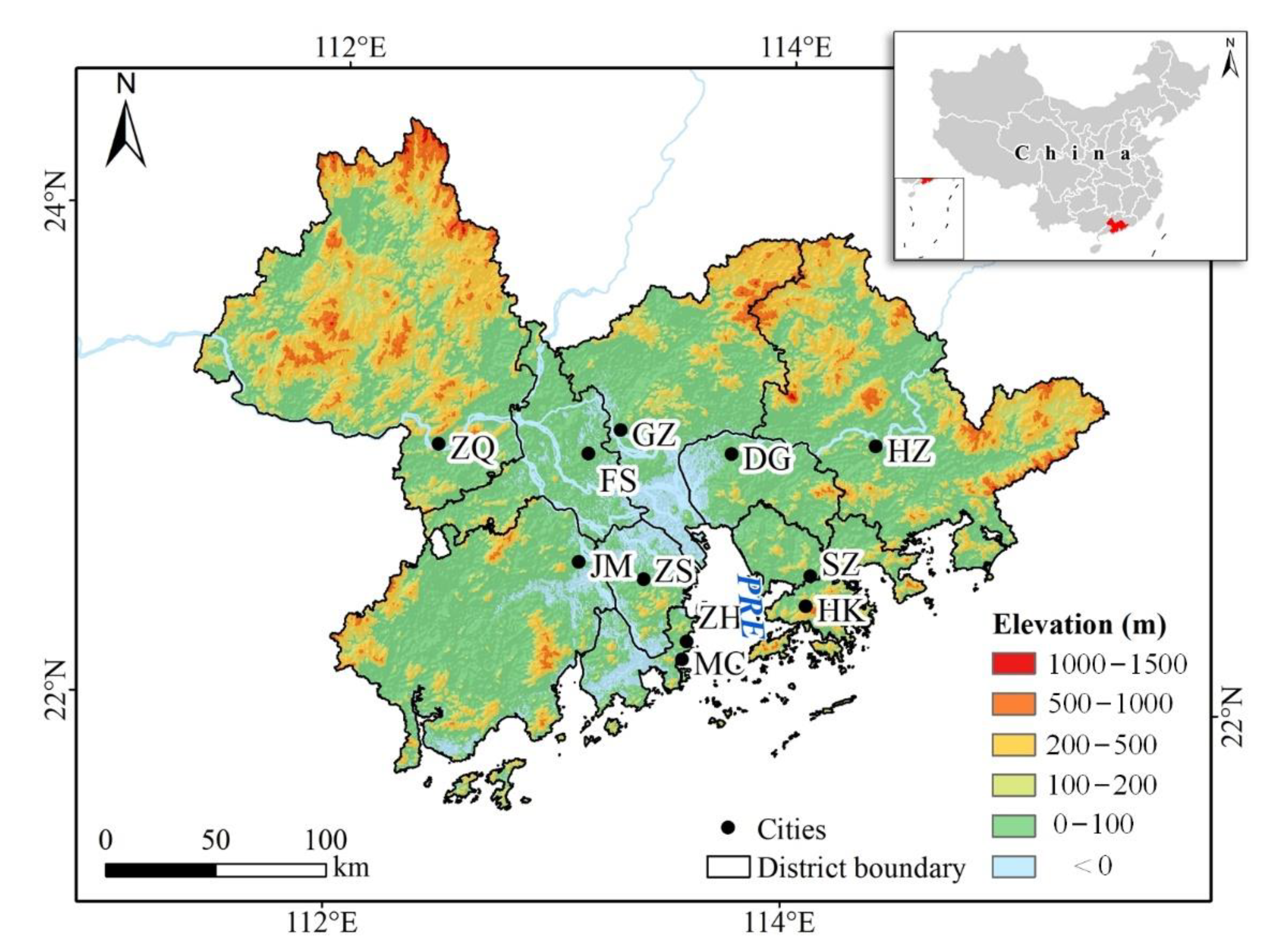
2.1. Study Area

The GBA, known as the Pearl River Delta urban agglomeration, is located in southern China and has an area of 55,000 km² (Figure 1). The GBA includes three separate customs territories, namely Guangdong, Hong Kong, and Macao, which include nine cities in Guangdong (Guangzhou, Dongguan, Huizhou, Shenzhen, Foshan, Zhongshan, Zhuhai, Jiangmen, and Zhaoqing), Hong Kong, and Macao, for a total of 11 cities. The GBA has a subtropical climate with a temperature of 22.3 °C/yr and rainfall of 1832 mm/yr. The central part of the study area is the alluvial plain of the Pearl River Delta, surrounded by hills in the west, north, and east. Diverse forest types distribute along with complex topography, including the broad-leaf forest, the mixed coniferous forest, and the mixed coniferous and broad-leaf forest [29]. As the constant freshwater resources and sediment are brought by the Pearl River system, the agriculture and aquaculture are well developed. The main crops in the study area are rice, sugar cane, sweet potatoes, soybean, peanut, banana, oranges, and lychee [30]. Since the implementation of China’s reform and opening-up policy, the GBA has been experiencing unprecedented urbanization and industrialization, transformed from a predominantly agricultural region into one of the developed areas in the world [26], and now plays an important strategic role in the development of the whole nation. However, extensive changes in land-use caused by human activities have severely impacted the structure, process, and functioning of local ecosystems, which has further led to the degradation of the ecosystem services and biodiversity.

2.2. Data Source

The land-use datasets of the study area were extracted from the Land-Use and Land Cover of China (CNLUCC) database in 1980, 1990, 2000, 2010, and 2018 [31]. The CNLUCC database was mainly produced by the object-oriented classification method and visual interpretation with the spatial resolution of 30 m, on the basis of a series of multi-source Landsat images, including Thematic Mapper (TM), Enhanced Thematic Mapper (ETM), and Operational Land Imager (OLI) images, as well as China-Brazil Earth Resources Satellite 1 (CBERS-1) data. Before interpretation, remote sensing images were geo-referenced based on 1:50,000 topographic maps and ortho-rectified. Ground control points (GCP) were applied for geometric rectification of remote sensing images. The root mean squared (RMS) error of geometric rectification was within 1.5 pixels (45 m). The Beijing 1954 Krasovsky Albers projection was used as the uniform coordinates and projection to integrate multiple temporal satellite images. In order to reduce the error caused by post-classification comparison, the outlines of land-use and land cover types were delimited by comparing remote sensing images between two years. The accuracy of the datasets was verified by using a great many of photographs obtained from historical data (aerial photos and interviews with local people), field survey, and unmanned aerial vehicle [32,33,34,35]. The CNLUCC is a multitemporal land-use database covering China and plays an important role in the investigation and research of national land resources, ecology, and hydrology.

The classification systems of the CNLUCC consist of 7 primary classes, namely, farmland, forest, grassland, water bodies, construction land, unused land, and seawater, and 22 subclasses. Based on this, a table of classification systems of ecosystems was built in this study (

Table 1. Classification systems of ecosystems based on the CNLUCC in the GBA.

Ecosystems		CNLUCC
Primary Classes	Subclasses	Subclasses	Codes
Farmland	Paddy field	Paddy field	11
	Dry farmland	Dry farmland	12
Forest	Forest	Forest	21
	Shrubs	Shrubs	22
	Shrubs	Sparse woods	23
	Shrubs	Other forestland	24
Grassland	Grassland	High-covered grassland	31
	Brush grass	Medium-covered grassland	32
	Meadow	Low-covered grassland	33
Water body	River system	Rivers and canals	41
	River system	Lakes	42
	River system	Reservoir pond	43
	River system	Seawater	99
Wetlands	Wetlands	Tidal flat	45
	Wetlands	Beach	46
	Wetlands	Marshland	64
Unused land	Desert	Sand	61
	Bare land	Bare land	65
	Bare land	Bare rock	66
Construction land		Urban residential area	51
		Rural residential area	52
		Other construction land	53

), including 7 primary classes: farmland, forest, grassland, water body, wetlands, unused land, and construction land. In addition, the statistical data of the study area are obtained from the Guangdong Provincial Statistical Yearbook and Census, Statistics Department of Hong Kong, and Statistics and Census Service of Macao.

2.3. Methods

2.3.1. Land-Use Dynamic Degree

The land-use dynamic degree was used to quantitatively examine the change rates of land-use types, and forecast the change trend of future land-use [36]. The degree of single land-use dynamics (K) was used to quantify changes in one specific ecosystem in this study. It can be expressed as the following formulas:

$$K=\frac{A_2-A_1}{A_1}\times \frac{1}{t}\times 100\%$$

(1)

where K refers to a specific ecosystem dynamicity in a study period; A₁ and A₂ represent the area of the specific ecosystem at the end time and the start time, respectively; and t is the study duration.

The comprehensive land-use dynamic degree (LC) was used to depict the overall dynamics of land-use of the study area in the study period, and it could be calculated as follows:

$$\mathrm{LC}=\frac{{{\displaystyle \sum }}_{i=1}^n\Delta A_{i-j}}{2\times {{\displaystyle \sum }}_{i=1}^n{A}_i}\times \frac{1}{t}\times 100\%$$

(2)

where LC refers to the comprehensive ecosystem dynamic degree; ΔA_i-j and A_i represent the conversion area from ecosystem i to ecosystem j from the start time to the end time, A_i is the area of ecosystem i at the start time; and t is the study time.

2.3.2. Intensity Analysis

Intensity analysis is a quantitative framework to analyze changes in terms of size and intensity at three levels based on transition matrix, namely, interval level, category level, and transition level [37,38,39]. The mathematical notation for intensity analysis is shown in

Table 2. The mathematical notation for Intensity Analysis.

Symbols	Meaning
J	Number of categories of ecosystems
i	A category at the initial time for a particular time interval
j	A category at the final time for a particular time interval
n	The gaining category in the transition of interest
T	Total time
t	The initial time of interval [Yt, Yt+1]
Yt	Year at time point t
Ctij	Size that transitions from category i at time Yt to category j at time Yt+1
St	Annual change intensity for time interval [Yt, Yt+1]
U	Value of uniform line for time intensity analysis
Gtj	Annual intensity of gross gain of category j for time interval [Yt, Yt+1]
Lti	Annual intensity of gross loss of category i for time interval [Yt, Yt+1]
Rtin	Annual intensity of transition from category i to category n during time interval [Yt, Yt+1] where i ≠ n
Wtn	Value of uniform intensity of transition to category n from all other categories at time Yt during time interval [Yt, Yt+1]

.

At the interval level, the total change in each time interval is analyzed to examine how the size and annual rate of change vary across time intervals.

$$\begin{array}{c}{S}_t=\frac{\mathrm{area} \mathrm{of} \mathrm{change} \mathrm{during} \mathrm{interval} [Y_t,Y_{t+1}]/\mathrm{area} \mathrm{of} \mathrm{study} \mathrm{region}}{\mathrm{duration} \mathrm{of} \mathrm{interval} [Y_t,Y_{t+1}]}\times 100\%\\ =\frac{\left\{{{\displaystyle \sum }}_{j=1}^J\left[\left({{\displaystyle \sum }}_{i=1}^J{C}_{tij}\right)-C_{tjj}\right]\right\}/\left[{{\displaystyle \sum }}_{j=1}^J\left({{\displaystyle \sum }}_{i=1}^J{C}_{tij}\right)\right]}{Y_{t+1}-Y_t}\times 100\%\end{array}$$

(3)

$$\begin{array}{c}U=\frac{\mathrm{area} \mathrm{of} \mathrm{change} \mathrm{during} \mathrm{all} \mathrm{intervals} /\mathrm{area} \mathrm{of} \mathrm{study} \mathrm{region}}{\mathrm{duration} \mathrm{of} \mathrm{all} \mathrm{intervals} }\times 100\%\\ =\frac{{{\displaystyle \sum }}_{t=1}^{T-1}\left\{{{\displaystyle \sum }}_{j=1}^J\left[\left({{\displaystyle \sum }}_{i=1}^J{C}_{tij}\right)-C_{tjj}\right]\right\}/\left[{{\displaystyle \sum }}_{j=1}^J\left({{\displaystyle \sum }}_{i=1}^J{C}_{tij}\right)\right]}{Y_T-Y_1}\times 100\%\end{array}$$

(4)

At the category level, each category is examined to measure how the size and intensity of both gross losses and gross gains varies across space.

$$\begin{array}{c}{G}_{tj}=\frac{\mathrm{area} \mathrm{of} \mathrm{gross} \mathrm{gain} \mathrm{of} \mathrm{category} j \mathrm{during} [Y_t,Y_{t+1}\left]/\mathrm{duration} \mathrm{of} [Y_t,Y_{t+1}\right]}{\mathrm{area} \mathrm{of} \mathrm{category} j \mathrm{at} \mathrm{time} Y_{t+1}}\times 100\%\\ =\frac{\left[\left({{\displaystyle \sum }}_{i=1}^J{C}_{tij}\right)-C_{tjj}\right]/\left(Y_{t+1}-Y_t\right)}{{{\displaystyle \sum }}_{i=1}^J{C}_{tij}}\times 100\%\end{array}$$

(5)

$$\begin{array}{c}{L}_{ti}=\frac{\mathrm{area} \mathrm{of} \mathrm{gross} \mathrm{loss} \mathrm{of} \mathrm{category} i \mathrm{during} [Y_t,Y_{t+1}\left]/\mathrm{duration} \mathrm{of} [Y_t,Y_{t+1}\right]}{\mathrm{area} \mathrm{of} \mathrm{category} i \mathrm{at} \mathrm{time} Y_t}\times 100\%\\ =\frac{\left[\left({{\displaystyle \sum }}_{i=1}^J{C}_{tij}\right)-C_{tii}\right]/\left(Y_{t+1}-Y_t\right)}{{{\displaystyle \sum }}_{i=1}^J{C}_{tij}}\times 100\%\end{array}$$

(6)

At the transition level, a particular transition is analyzed to examine how the size and intensity of the transition varies among other categories for that transition.

$$\begin{array}{c}{R}_{tin}=\frac{{\mathrm{area} \mathrm{of} \mathrm{transition} \mathrm{from} i \mathrm{to} n \mathrm{during} [\mathrm{Y}}_{\mathrm{t}}{,\mathrm{Y}}_{\mathrm{t}+1}{]/\mathrm{duration} \mathrm{of} [\mathrm{Y}}_{\mathrm{t}}{,\mathrm{Y}}_{\mathrm{t}+1}]}{{\mathrm{area} \mathrm{of} \mathrm{category} i \mathrm{at} \mathrm{time} \mathrm{Y}}_{\mathrm{t}}}\times 100\%\\ =\frac{C_{tin}/\left(Y_{t+1}-Y_t\right)}{{{\displaystyle \sum }}_{i=1}^J{C}_{tij}}\times 100\%\end{array}$$

(7)

$$\begin{array}{c}{W}_{tn}=\frac{{\mathrm{area} \mathrm{of} \mathrm{gross} \mathrm{gain} \mathrm{of} \mathrm{category} n \mathrm{during} [\mathrm{Y}}_{\mathrm{t}}{,\mathrm{Y}}_{\mathrm{t}+1}{]/\mathrm{duration} \mathrm{of} [\mathrm{Y}}_{\mathrm{t}}{,\mathrm{Y}}_{\mathrm{t}+1}]}{{\mathrm{area} \mathrm{that} \mathrm{is} \mathrm{not} \mathrm{category} n \mathrm{at} \mathrm{time} \mathrm{Y}}_{\mathrm{t}}}\times 100\%\\ =\frac{\left[\left({{\displaystyle \sum }}_{i=1}^J{C}_{tin}\right)-C_{tnn}\right]/\left(Y_{t+1}-Y_t\right)}{{{\displaystyle \sum }}_{j=1}^J\left[\left({{\displaystyle \sum }}_{i=1}^J{C}_{tij}\right)-C_{tnj}\right]}\times 100\%\end{array}$$

(8)

2.3.3. Assessment of the Ecosystem Service Value

According to previous studies [1,3,18], the ESV of the GBA was calculated as follows:

$$\mathrm{ESV}={\displaystyle \sum }\left(A_k\times V_{ck}\right)$$

(9)

where ESV denotes the total annual value of the ecosystem services, and A_k and V_ck are the area and value coefficient for ecosystem type k, respectively.

To obtain more accurate ESV, the main grain yield was used to revise the ecosystem services equivalent value in this study, and more details have been provided in our previous study [6]. In this study, the ESV of each ecosystem was calculated as the sum of the ESVs of its own sub-ecosystems. For example, the total ESV of farmland is the sum of the ESVs of both paddy fields and dry farmland. In this study, ecosystem services included 11 categories [1,18], namely, food production, nutrient cycling, water supply, gas regulation, climate regulation, environmental purification, hydrological regulation, soil conservation, nutrient cycling, biodiversity conservation, and recreational and aesthetic values. The ESV of these 11 categories was also calculated. In addition, the ESV of construction land was regarded as 0 in this study.

3. Results

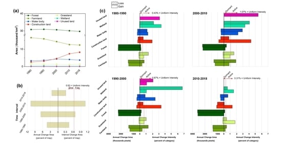
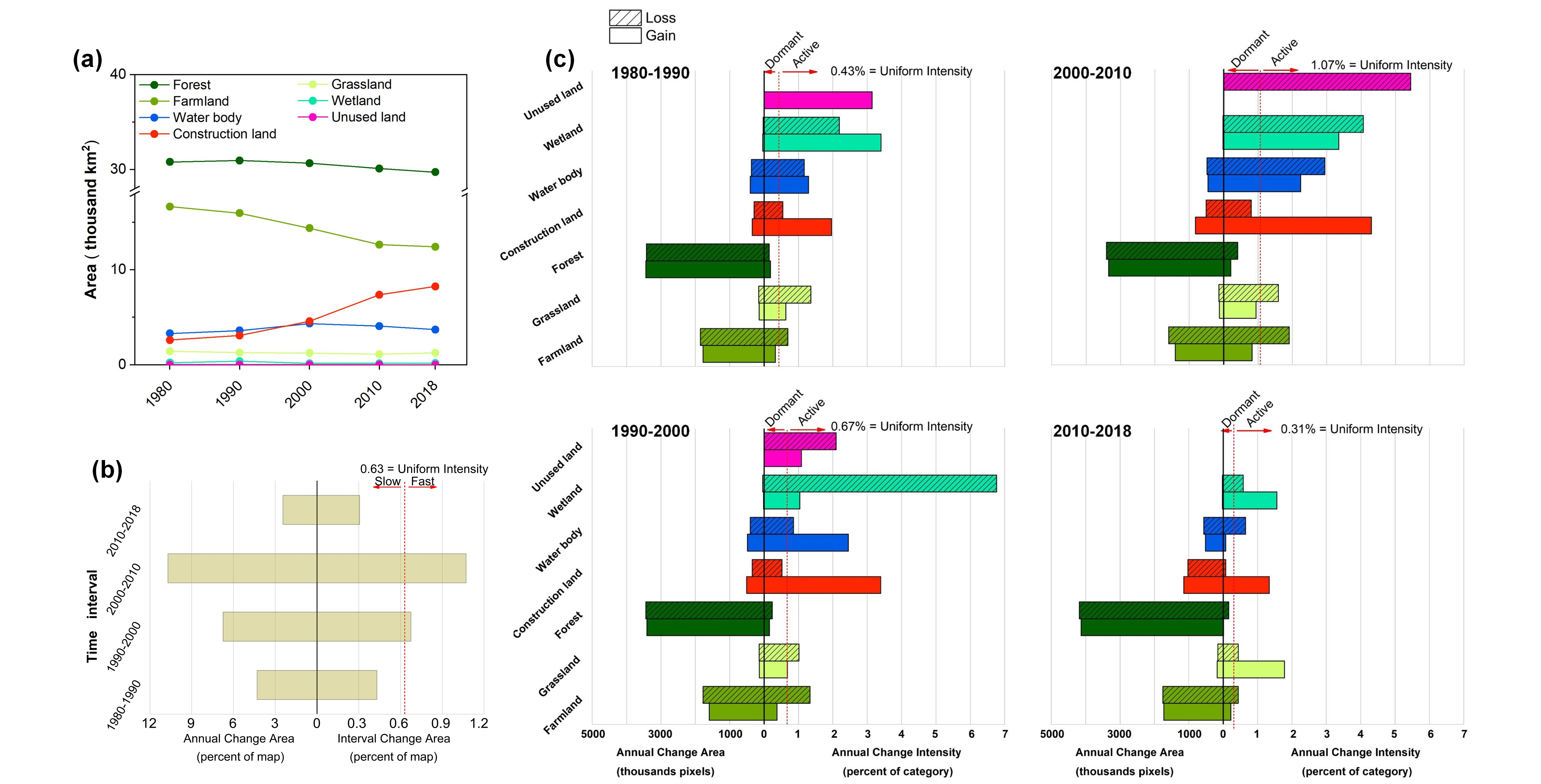
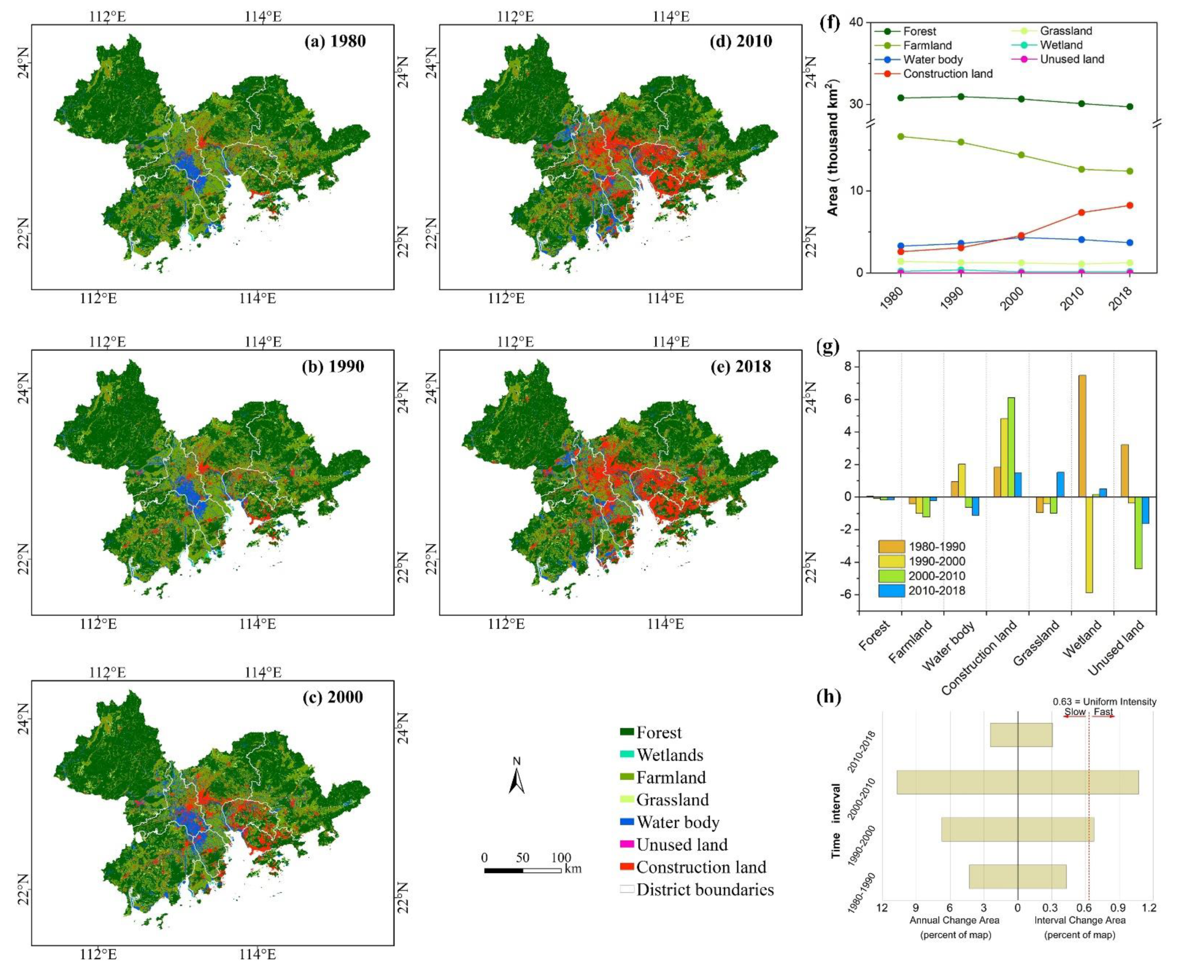
3.1. Spatial and Temporal Changes in Different Ecosystems

The spatial distributions of 7 different ecosystems in the GBA from 1980 to 2018 are displayed in Figure 2a–e. Forest ecosystems are mainly distributed in the northern, eastern, and western parts of the GBA with higher elevations, such as Zhaoqing, Huizhou, and Jiangmen, while farmland and construction land are mostly located in flat areas, such as the Pearl River Delta Plain. Over the whole study period, it was notable that an extensive expansion of construction land occurred in the study area. Plaque-like patches with large areas of construction land were observed in Guangzhou, Dongguan, Shenzhen, and Foshan by 2018, while they were only sporadically scattered in 1980. In addition, a large water body located at the junction of Foshan, Zhongshan, and Jiangmen suddenly disappeared in 2010; instead, farmland and construction land appeared here (Figure 2d).

The area changes for different ecosystems show distinctive patterns (Figure 2f). Forest ecosystems are the most dominant type of ecosystem in the GBA, and their area displayed an almost indistinguishable trend over the past 40 years, with initial percentages from 56% to 54%. In contrast, the area of farmland showed a clear decrease from 16,640 km² in 1980 to 12,417 km² in 2018. Such a decrease was mostly at the expense of an increase in the area of construction land, which had almost twice the growth throughout the study period. For water bodies and wetlands, a unimodal pattern was observed, with peaks appearing in 2000 and 1990, respectively. The changes in the area of grassland exhibited an overall decrease with a slight increase in the last study period. Distinctive patterns were also observed for K, which was used to reflect the degree of changes in a single ecosystem (Figure 2g). The K of construction land was monotonically positive in different study periods, which contrasted with the monotonic negativity exhibited by farmland. Nevertheless, the highest K of both construction land and farmland occurred from 2000 to 2010, followed by the period from 1990 to 2000. The K of forest and unused land was positive in the first study period and negative in the other three study periods; nonetheless, such a trend was more notable for unused land. For water bodies, the value of K was positive and negative in the first two decades and the last two decades, respectively. A negative K was observed for grassland in the former three study periods, and then a positive K appeared in the last period. The K of wetlands differed significantly throughout the study periods, surpassing 7% from 1980 to 1990 and almost −6% from 1990 to 2000, followed by two positive values of less than 0.6%.

With regard to time interval level intensity analysis, bars extending to the left from 0 show gross area of overall changes within each time interval, while bars extending to the right from 0 show intensity of annual area of change in each interval (Figure 2h). The same was observed for the annual change area and interval change area, namely, the size of the change and land change rate during the third time interval was the biggest and fastest, followed by the second time interval.

The category level intensity analysis in the study area was displayed in Figure 3. The left side of Figure 3 shows that forest and farmland have relatively larger size in terms of both annual losses and gains during the four time intervals, and losses are a little bit larger than gains. However, the right side of Figure 3 shows that the intensities of forest’s losses and gains are dormant, which is mainly because they account for a large area percentage of the study area. The intensity of losses and gains of the wetland are active, due to the small size. Besides, the activity intensity within the categories also plays important roles. The bar for the gains of the construction land extends to the right of the uniform line in the four time intervals, which illustrates that construction land experiences gains much more intensively than the landscape in general. Similarly, the bar for loss of farmland extends to the right of the uniform line in the four time intervals, which illustrates that farmland experiences losses more intensively than the landscape in general.

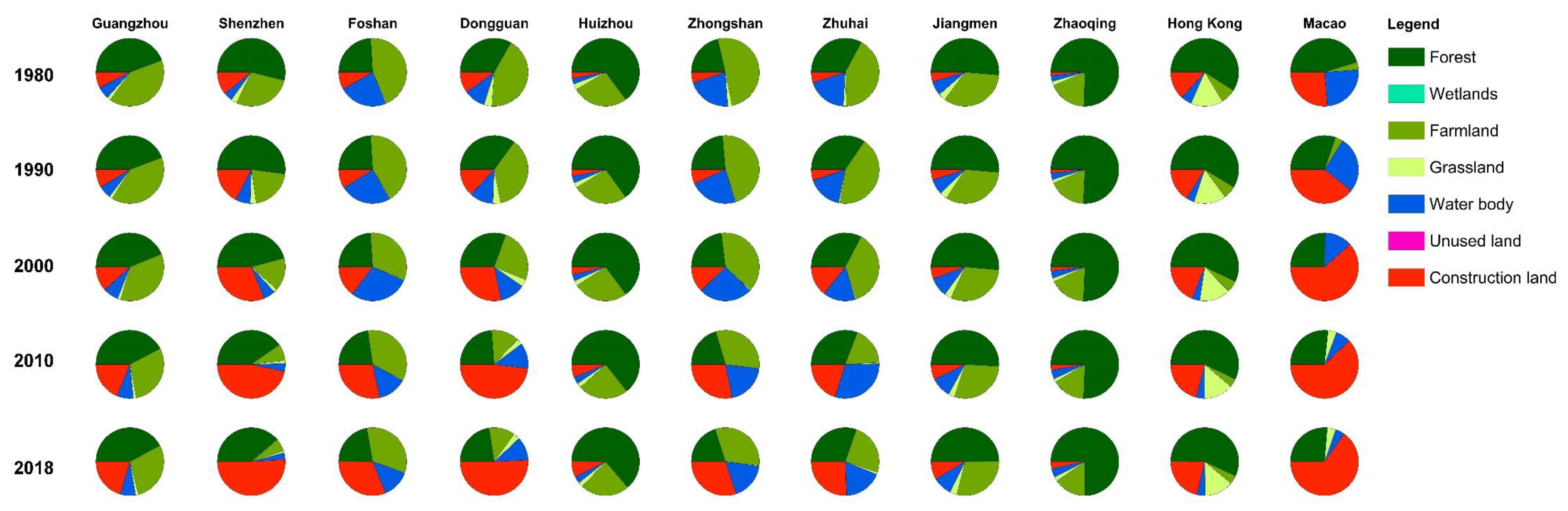
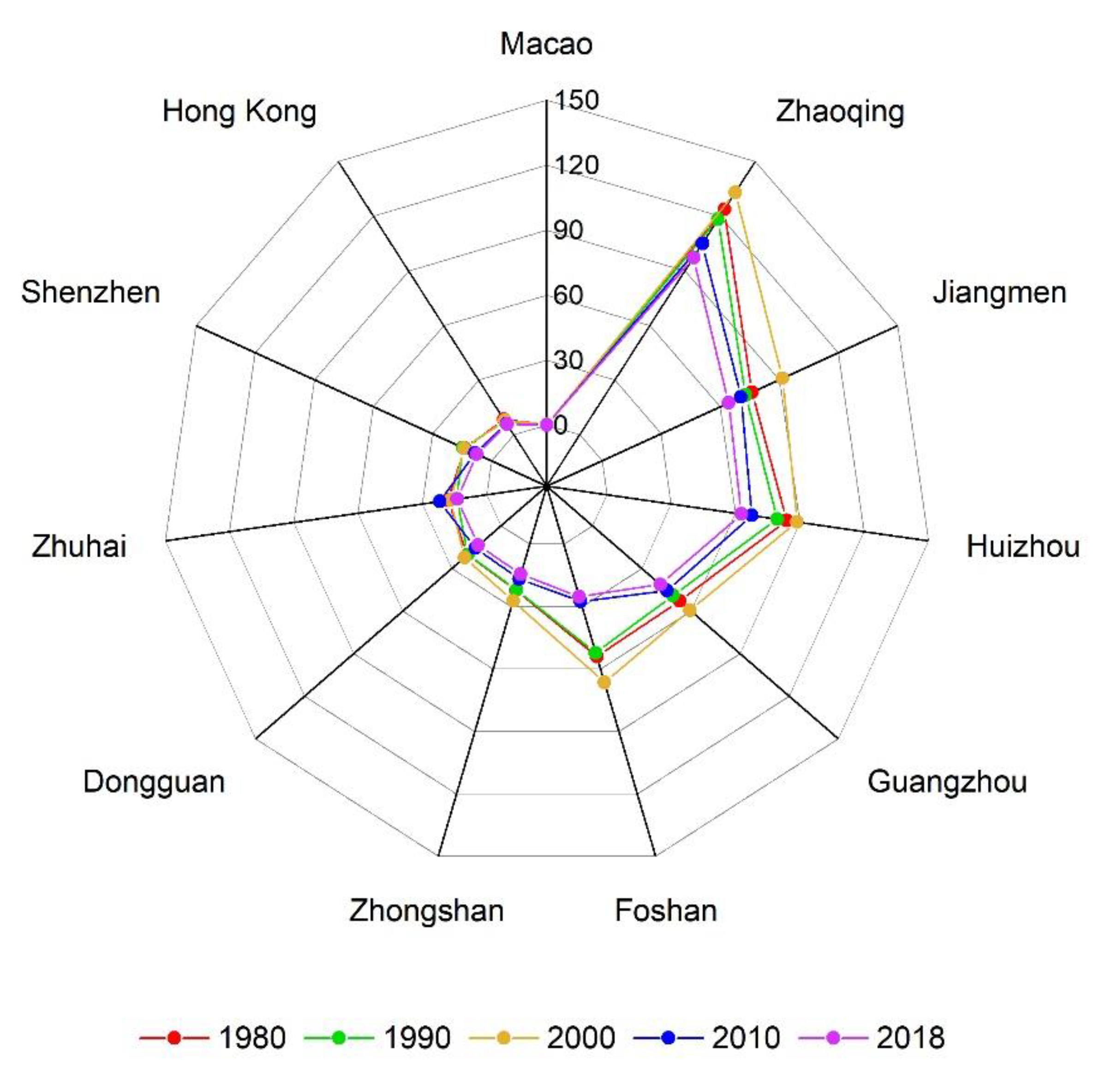
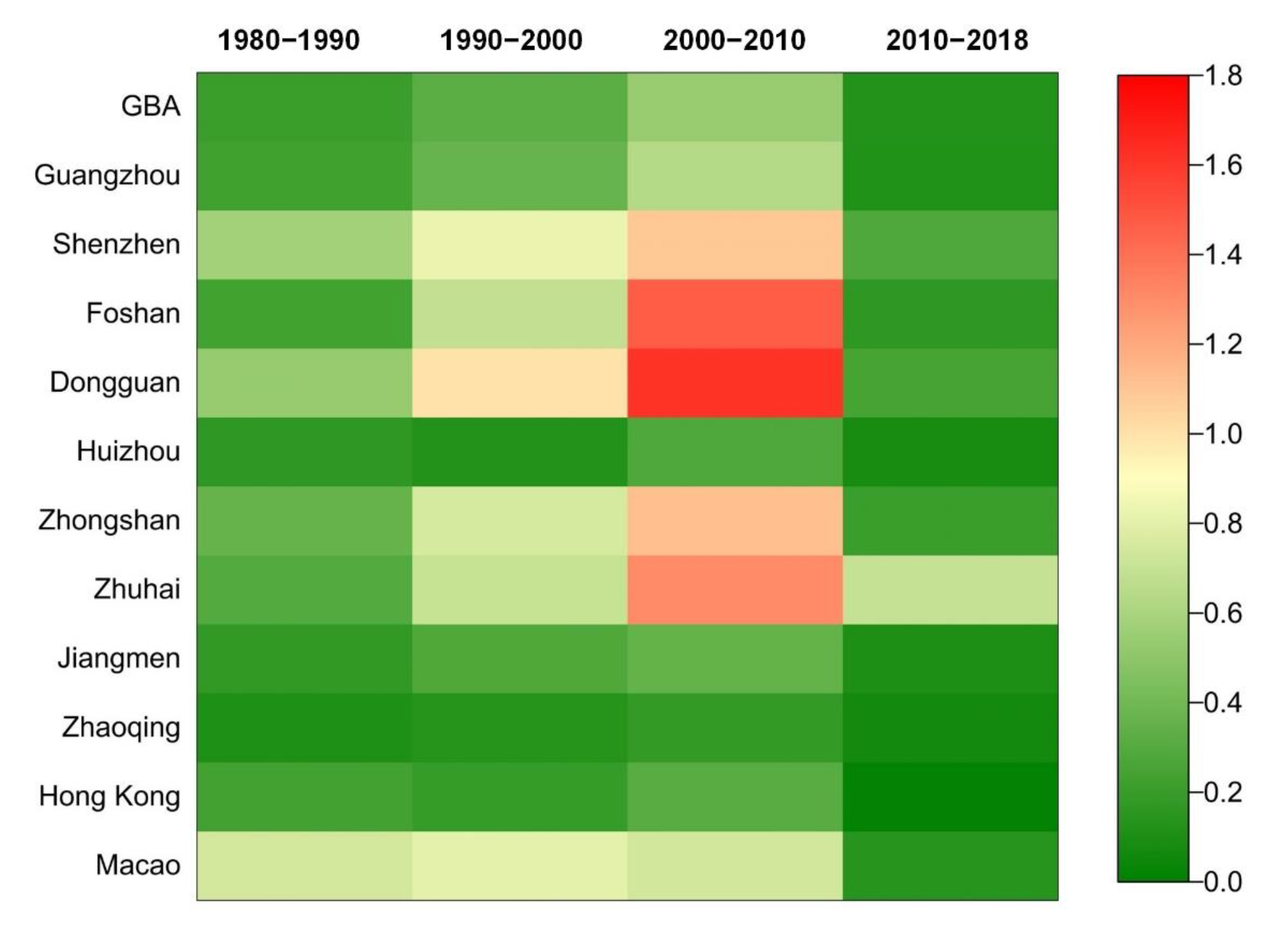
3.2. Changess in Regional Ecosystems

The combination of ecosystems varied significantly to a regional extent, although the main ecosystem categories were forest, farmland, construction land, and water bodies (Figure 4). Over the past 38 years, the area percentage of different ecosystems did not exhibit any discernible trend in Jiangmen, Zhaoqing, and Hong Kong; nonetheless, in other areas, construction land expanded dramatically, and farmland showed a significant decrease. In addition, the forest cover degree was over 45% in Zhaoqing, Huizhou, Hong Kong, Jiangmen, Guangzhou, and Shenzhen, throughout the study period.

The LC of the GBA and 11 cities is displayed as a heat map in Figure 5, which showed distinctive patterns during the study periods. The LC of the GBA was relatively low, with the highest value (0.5%) occurring from 2000 to 2010. Similar trends were also observed in Guangzhou, Huizhou, Jiangmen, Zhaoqing, and Hong Kong. The LC in Shenzhen, Foshan, Dongguan, Zhongshan, and Zhuhai was relatively high, especially in Dongguan from 2000 to 2010, with the highest value of 1.6%. In addition, the LC in the whole GBA was dark green or green from 2010 to 2018, which indicated that the comprehensive ecosystem changes slowed down.

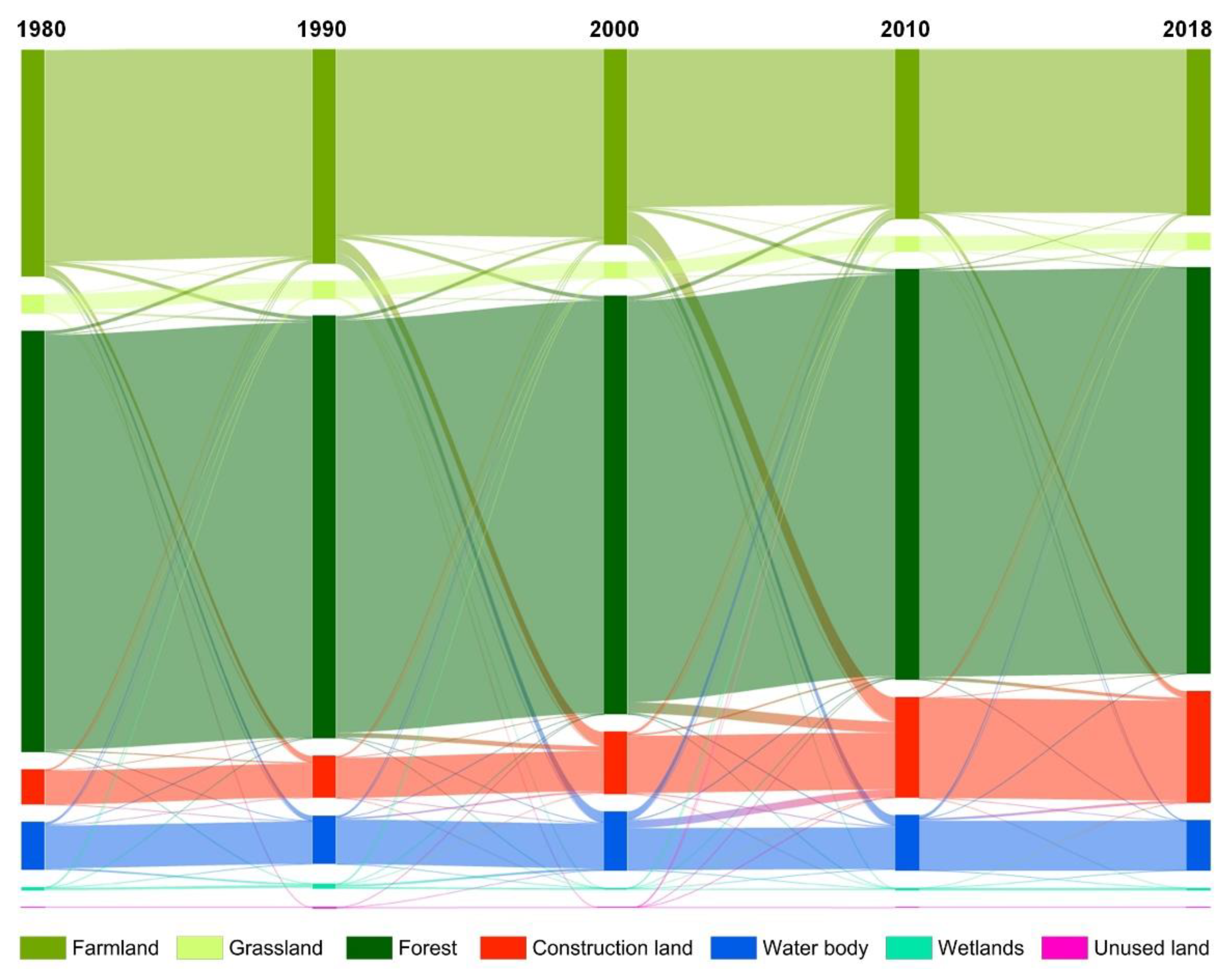
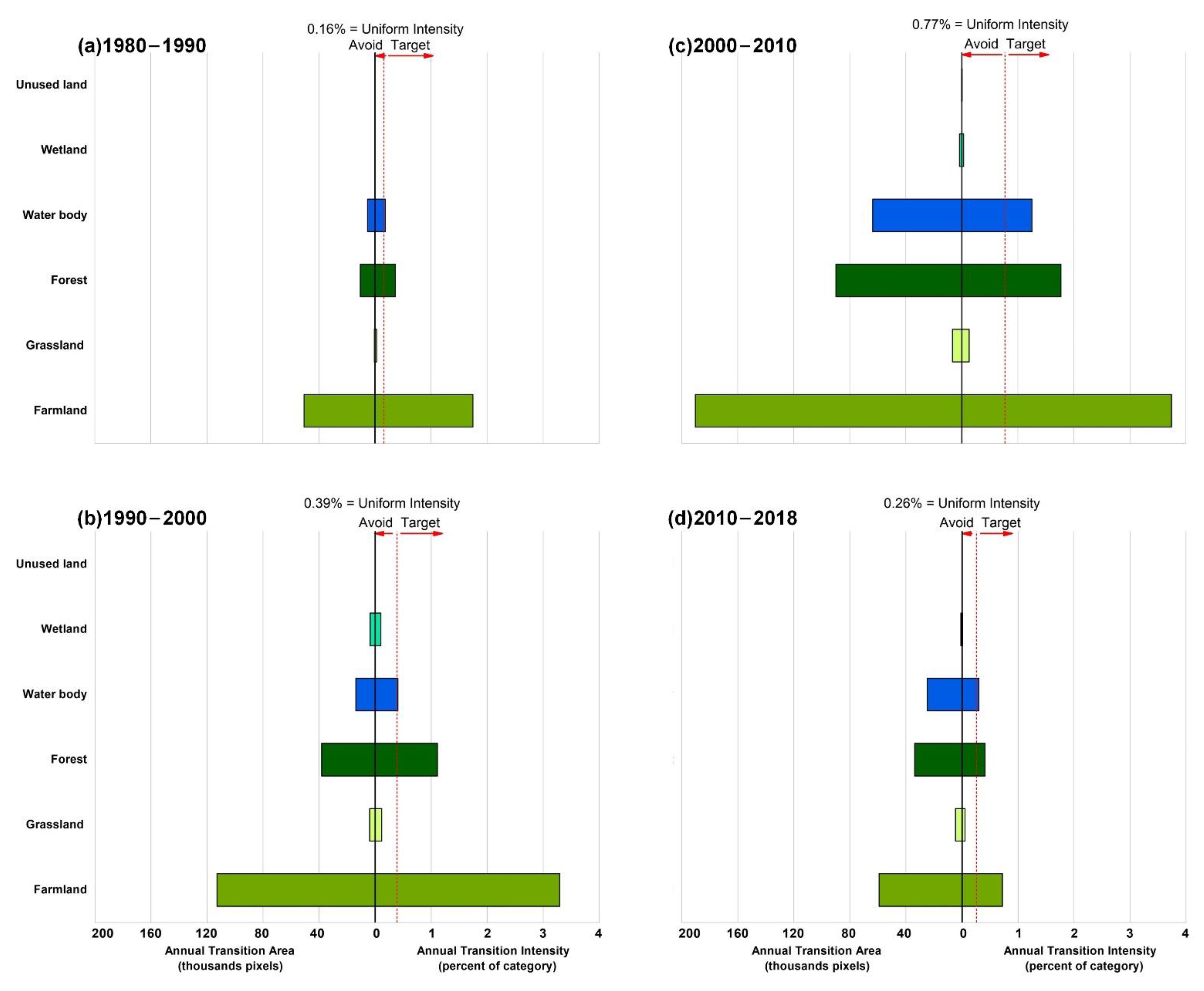
3.3. Conversions among Different Ecosystems

The conversions among these seven ecosystems were conducted to quantitatively study the number and direction of different ecosystem categories, and the results were displayed by a Sankey diagram (Figure 6). In the four study periods, the total converted areas were 2377 km², 3731 km², 5925 km², and 1360 km², respectively. From 1980 to 1990, the farmland ecosystem suffered the most loss, with an area decrease of 1148 km², and most of this land was converted to construction land (39.7%), water bodies (32.8%), and forest (25.7%). Furthermore, construction land, forest, farmland, and water bodies gained more areas from other ecosystem types, with areas of 606 km², 565 km², 523 km², and 468 km², respectively. A similar change trend of farmland ecosystems was observed from 1990 to 2000, in which the area decreased by 2136 km², mostly encroached by construction land (47.6%) and water bodies (37.7%). Correspondingly, the areas of new construction land and water bodies were relatively higher, with increases of 1552 km² and 1064 km², respectively. From 2000 to 2010, conversion from farmland ecosystems to other ecosystems was still the most significant, with a conversion area of 2742 km², followed by that of forest with an area of 1265 km², and that of water bodies with an area of 1280 km². Meanwhile, the area of construction land gained from other ecosystems was the highest (3172 km²), followed by farmland (1049 km²). A similar change was observed from 2010 to 2018, but it exhibited almost indistinguishable changes.

The intensity analysis at transition level for gains of construction land is shown in Figure 7. The gain of construction land originated mainly from farmland, followed by forest, and water body in four time intervals. The transition intensity is strongest in 2000–2010, followed by that in 1990–2010.

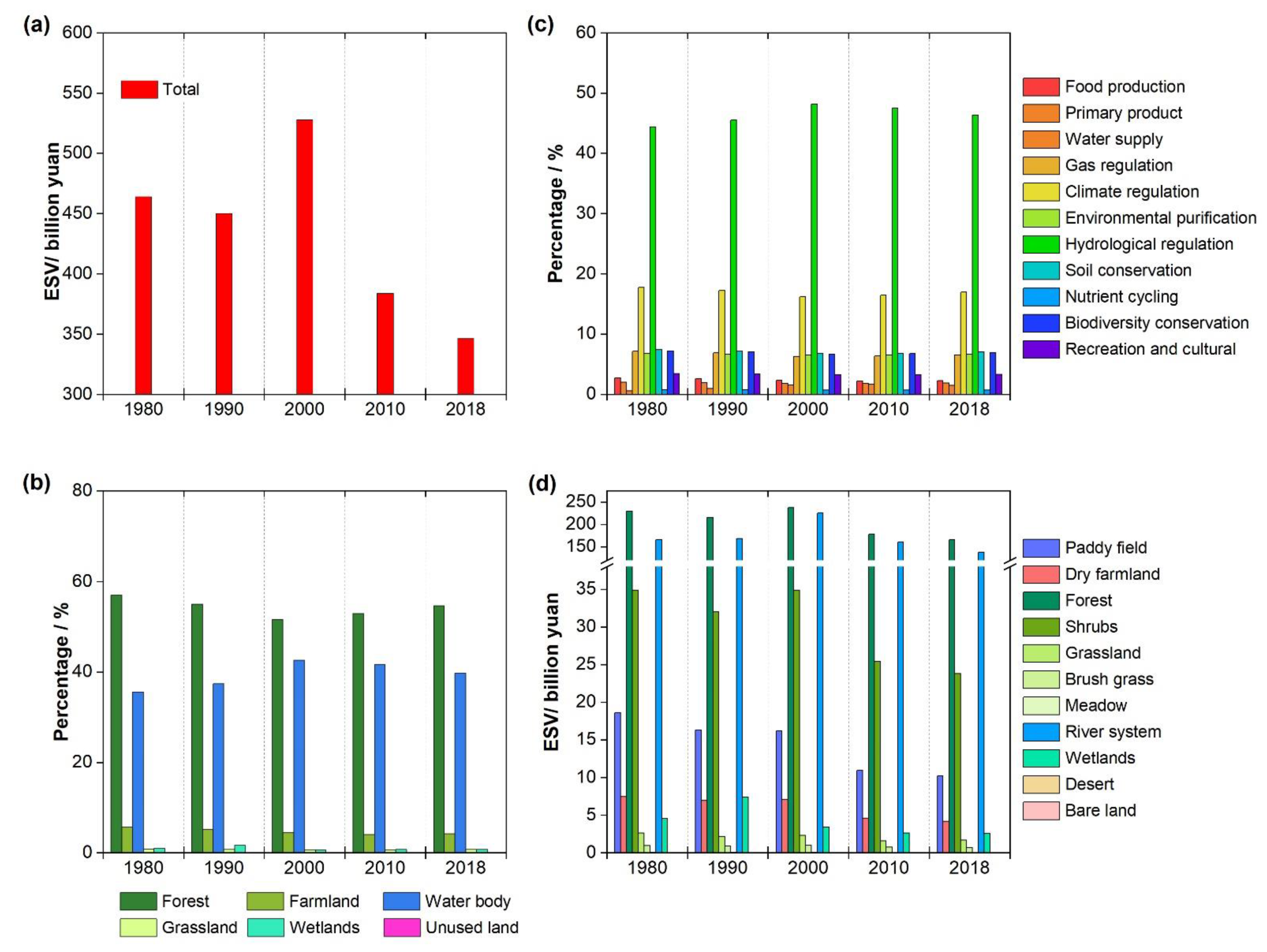
3.4. Changes in Ecosystem Services

The changes in the total ESV of the GBA in different study periods are displayed in Figure 8. The total ESV showed an overall declining trend throughout the study periods except in 2000, declining from 464 billion yuan to 346 billion yuan (Figure 8a). The highest ESV was 528 billion yuan in 2000, which was mainly because of the largest area of water bodies at that time. Regarding the different ecosystems, the ESV provided by the forest ecosystem made the greatest contribution to the total ESV in the GBA, followed by that provided by water body ecosystem throughout the study period (Figure 8b). The ESV of forest ecosystems and water body ecosystems contributed more than 92% to the overall ESV in each study period. The influence of the ESV provided by forest ecosystems decreased from 57% in 1980 to 52% in 2000, and then increased to 55% by 2018. In contrast, the proportion of the ESV of the water body ecosystem showed a growth trend, from an initial value of 36% in 1980 to 43% in 2000, and then it declined to 40% by 2018. Although the area of farmland ecosystems was far more than that of water body ecosystems, the ESV provided by the former was far less than that of the latter. The total contribution of grassland, wetlands, and unused land was less than 2.3% during the study period. Among all ecosystem service functions, the influence of hydrological regulation was the largest, ranging from 44% to 48% (Figure 8c) in the past four decades, followed by that of climate regulation (ranging from 16% to 18%). The contributions of gas regulation, environmental purification, soil conservation, and biodiversity conservation were comparable and showed little change from 1980 to 2018. In addition, the highest ESV of most ecosystem services was observed in 2000. In terms of the subclass ecosystems, the ESV of forests and rivers has dominant positions with an overall decline trend throughout the study periods (Figure 8d). The ESV of paddy fields made more contributions to the total ESV of farmland than that of the dry farmland, even though both of them decreased in the past forty years. The ESV of wetlands is largest from 1990 to 2000, then it declined.

The ESV changes of the 11 cities over the various study periods are displayed in Figure 9. Similar trends with the total ESV changes in the GBA were observed in the changes in regional ESV. The largest ESV in most cities was observed in 2000, and the minimum value was observed in 2018. Among the 11 cities, the ESV in Zhaoqing was always the largest in the different study periods, ranging from 97 billion yuan to 133 billion yuan. In a clockwise direction starting from Zhaoqing to Macao, an overall decreasing trend of regional ESV was observed. From Zhongshan to Macao, the ESVs in all 6 cities were less than 30 billion yuan from 1980 to 2018. The ESV in Foshan was also below 30 billion yuan after 2010.

4. Discussion

4.1. Changes in Ecosystems

The present study reveals that the ecosystem structure in the GBA experienced dramatic changes from 1980 to 2018, and the most pronounced changes were construction land expansion and farmland loss, with areas varying from 2607 km² to 8244 km² and from 16,640 km² to 12,417 km², respectively. Meanwhile, the area of forest, water bodies and wetlands showed unimodal patterns. During the four adjacent periods, construction land was the main ecosystem category converted from other types, with increasing influences of 26%, 42%, 54%, and 65%, respectively. In contrast, farmland was always the main ecosystem that was converted into other ecosystem types, with contributions of 48%, 57%, 46%, and 33%, respectively, followed by forest and water bodies with increasing contributions. Our results are highly consistent with previous research, indicating that rapid urbanization has become the main reason for the loss of farmland, forest, water bodies, and wetlands [8,9,11,40,41]. Due to the close geographical location, new increased construction land mainly originates from the conversion of farmland, resulting in farmland suffering the most loss [6,8,28]. Substantial farmland loss is increasingly threatening food security and farmland preservation under the effects of construction land expansion. First, the requisition–compensation balance of farmland has been heavily impacted. Substantial high-quality farmland has been lost because of construction land sprawl, but the compensatory farmland is mainly characterized by low quality and low productivity [7,42,43,44]. Second, construction land expansion has caused patches of farmland to become more isolated and fragmented [42,45]. Multiple effects of urbanization on farmland have resulted in an increase in agricultural activity intensity and pesticide use to meet the demand for food supply, which has threatened food security and farmland preservation and has caused serious widespread water and soil pollution, and biodiversity loss [9,46,47,48,49]. In addition, Jiang et al. implied that continued urbanization might stimulate farmland expansion, which will impose high pressure on natural landscapes and ecosystems in the future [9]. Our results supported this finding, and the new increase in farmland coupled with construction land expansion mainly resulted in the degradation of forest and water body ecosystems throughout the study period. The loss and degradation of forests, water bodies, and wetlands have severe impacts on global environmental change, ecosystem services, natural habitat, and biodiversity loss [10,11,41].

4.2. Changes in Ecosystem Services

The ESV in the GBA exhibited an overall decrease from 464 billion yuan in 1980 to 346 billion yuan in 2018 (Figure 8a). This result was essentially driven by the ESV changes in forest and water bodies with contributions of 52%–57% and 36%–43%, respectively (Figure 8b). Our results proved that forests and water bodies play vital roles in regulating ecosystem services and ecosystem functions in the study area, because forest has the largest area (ranging from 54% to 56%) and water bodies have the highest ESV per unit area (ranging from 37.1 million yuan/km² to 50.2 million yuan/km²). This is also the reason for the significant spatial heterogeneity of the ESV in the GBA, namely, the total ESV of Zhaoqing is always the highest, followed by that of Jiangmen and Huizou (Figure 9), which is mainly because they have higher forest or water cover areas and rates. With respect to ecosystem services provided by ecosystems, forest not only provides raw materials, including wood, fiber, and fuelwood, but also can store atmospheric carbon dioxide and moderate regional climate, which is essential for human well-being [50]. In addition, forest ecosystems can purify water, degrade plant litter and animal wastes, and create or regenerate fertile soils, which is vital for subsistence slash-and-burn farming systems [51]. This may explain why the new increased farmland in the GBA was mainly converted from forest throughout the study period (Figure 6). The main ecosystem service provided by farmland is its provisioning services dominant by food, and fiber, depending on critical ecosystem services, such as soil fertility, pollination, and pest control. Pollinators, seed dispersers, and pest control agents, make significant contributions to 35% of the world’s crop production, taking natural or semi-natural ecosystems as important nesting locations and additional food sources [50,52]. However, extensive urbanization has encroached substantial natural or semi-natural ecosystems, which further affects biodiversity [10,11]. Wild bees (e.g., Hymenoptera, Apidae, Bombus spp.) are important pollinators within the agricultural and forest ecosystems, whose population are declining [53,54]. Additionally, as substantial farmland was lost because of urbanization, the service of food production provided by farmland ecosystem suffered negative effects with the total output of major grain crops in the GBA showing a declining trend throughout the study period (Figure 10). Hence, urbanization has directly and indirectly resulted in the dramatic reduction and degradation of ecosystem services with unpredictable and even unrecoverable damages and influences.

4.3. Drivers of the Changes

Our results in this study indicated that construction land expansion was the direct factor driving the dramatic changes in ecosystems and their services. which was highly consistent with previous studies [4,8,55,56,57,58,59]. In terms of indirect factors, previous research has demonstrated that urbanization is the essential result of population explosion, economic growth, and policy guidance [30,60,61,62]. We consider that the geographic location is also an important factor, namely, for urbanization, the basic factor is geographic location, the guidance is policy, and the driving forces are economic growth and population explosion. The GBA is located in the Pearl River Delta with abundant water resources and fertile soils, and the area used to be a predominantly agricultural region [26,63]. Since it is adjacent to Hong Kong and Macao along the South China Sea, it plays an important role in the development of the local economy and in the construction of the Belt and Road. The basic geographic location determines its strategic situation; thus, it was chosen as one of the pilot areas of the reform and opening-up policy implemented in 1978. Subsequently, Deng Xiaoping conducted his tour in the south (Nanxun) in 1992 and visited Shenzhen and Zhuhai, stimulating local development. The government of Guangdong Province established the Pearl River Delta Economic Zone in 1994 to further promote regional development. Later, the Hong Kong and Macao Special Administrative Regions were built in 1997 and 1999, respectively. In 2001, China joined the World Trade Organization, and an increasing number of enterprises at home and abroad settled in the study area. By 2017, the GBA was established to comprehensively promote mutually beneficial cooperation among the mainland, Hong Kong, and Macao. A series of policies above guided and accelerated the conversion from a predominantly agricultural region into one of the most developed areas [26]. Furthermore, increasing economic strength can provide sufficient financial support for the expansion of construction land; however, as the population of secondary and tertiary industry increasingly grow (Figure 11a), more construction land is needed to support the development of secondary and tertiary industries, such as building more factories for manufacturing and services [60,62]. Economic development needs and absorbs a large labour force, resulting in rapid urban population growth, as well as its proportion (Figure 11b), which places significant demands on societies’ ability to provide public services such as adequate housing, which directly stimulates the expansion of construction land [64]. Overall, multiple factors, including geographic location, policy, economic growth, and population growth, contributed to the development of urbanization and industrialization, which induced dramatic changes in local ecosystems and degradation of ecosystem services and ecosystem functions.

4.4. Suggestions for Sustainable Development

This study showed that the GBA has undergone dramatic changes in ecosystem structure in the past four decades, resulting in significant changes in various ecosystem services, which were mainly caused by the expansion of construction land. Nevertheless, continued urbanization will also impact natural ecosystems and ecosystem services in the future. Ecosystems diversity, including habitats diversity and species richness, show higher levels of multiple ecosystem functions, which has the greatest impact on human health and well-being benefits [65,66]. Sustaining and enhancing human well-being requires a balance of all of our assets, including the built economy, society, individual people, and ecosystems [3]. To respond to the SDGs of the United Nations to protect and promote the sustainable use of terrestrial ecosystems, we propose several suggestions for the sustainable development of the GBA based on the results of this study:

(1) Protect natural ecosystems to realize sustainable development. Narrowly speaking, sustainable development refers to efficiently protecting the environment and natural resources during economic development [67]. Here, we advise that governments draft and implement strict and efficient policies to control the encroachment of construction land on natural ecosystems and protect, restore, and promote the sustainable use of high-quality farmland, forest, water bodies, and wetlands.

(2) Strictly control the area of new construction land, especially the area of impermeable surfaces, during the process of urbanization in the near future. Construction land sprawl not only encroached substantial natural ecosystems but also caused further dramatic degradation of ecosystem services and functions. We suggest that governments scientifically plan the distribution, strictly control the area of new construction land, and encourage the use of permeable materials rather than impermeable materials to build artificially hardened surfaces, such as roads.

(3) Scientifically plan the distribution of different ecosystems throughout the GBA to weaken the uneven spatial distribution of ESV. Since the total ESVs of Zhaoqing, Huizhou, and Jiangmen were much higher than those of Zhuahai, Shenzhen, and Dongguan, we recommend that governments relocate some factories for manufacturing and services from the latter to the former and protect and restore the forests, wetlands, and water bodies—such ecosystems with higher ESVs in more developed areas.

5. Conclusions

The GBA has been experiencing unprecedented urbanization and industrialization since the implementation of China’s reform and opening-up policy in 1978, significantly influencing local ecosystems. To raise awareness of the importance of ecosystems and their services, the historical changes in ecosystem structure in the GBA from 1980 to 2018 were investigated based on a series of land-use datasets, and the ESV was quantified using monetary units in different study periods in this study. The results showed that drastic changes were observed in the ecosystem structure, especially for farmland, with the largest decrease of 4223 km², and construction land, with the highest increase of 5636 km². Forest and farmland have relatively larger size with respect to both annual losses and gains during four time intervals. The largest LC (1.6%) was observed in Dongguan from 2000 to 2010, and it was low in the whole GBA and 11 cities from 2010 to 2018, which indicated that the local ecosystems suffered less disturbance from human activities at that time. An overall decrease in the total ESV of the study area was observed, declining from 464 billion yuan in 1980 to 346 billion yuan in 2018. The ESV supported by forest ecosystems contributed the most to the total ESV, ranging from 52% to 57%, followed by water body ecosystems with 36%–43%. With respect to ecosystem service functions, hydrological regulation and climate regulation suffered the most effects due to ecosystem structure changes. In addition, the ESV displayed significant spatial heterogeneity in the 11 cities, with lower values in the central region and higher values in the surrounding region. To realize the sustainable development of the GBA, we suggest that local governments strictly control the impacts of human activities on natural ecosystems and scientifically use and protect forests, farmlands, water bodies, and wetlands as important ecosystems. Our future work will quantitatively study the relationship between ecosystem services and sustainable development by building a sustainable land-use comprehensive evaluation model.

References

1. Costanza, R.; d’Arge, R.; de Groot, R.; Farber, S.; Grasso, M.; Hannon, B.; Limburg, K.; Naeem, S.; O’Neill, R.V.; Paruelo, J.; et al. The value of the world’s ecosystem services and natural capital. Nature 1997, 387, 253–260. [Google Scholar] [CrossRef]
2. Millennium Ecosystem Assessment. Ecosystems and Human Well-Being: Synthesis; Island Press: Washington, DC, USA, 2005. [Google Scholar]
3. Costanza, R.; de Groot, R.; Sutton, P.; van der Ploeg, S.; Anderson, S.J.; Kubiszewski, I.; Farber, S.; Turner, R.K. Changes in the global value of ecosystem services. Glob. Environ. Chang. 2014, 26, 152–158. [Google Scholar] [CrossRef]
4. Estoque, R.C.; Murayama, Y. Landscape pattern and ecosystem service value changes: Implications for environmental sustainability planning for the rapidly urbanizing summer capital of the Philippines. Landsc. Urban Plan. 2013, 116, 60–72. [Google Scholar] [CrossRef]
5. Xiao, R.; Lin, M.; Fei, X.; Li, Y.; Zhang, Z.; Meng, Q. Exploring the interactive coercing relationship between urbanization and ecosystem service value in the Shanghai-Hangzhou Bay metropolitan region. J. Cleaner Prod. 2020, 253, 119803. [Google Scholar] [CrossRef]
6. Wang, X.; Yan, F.; Su, F. Impacts of urbanization on the ecosystem services in the Guangdong-Hong Kong-Macao greater bay area, China. Remote Sens. 2020, 12, 3269. [Google Scholar] [CrossRef]
7. Song, W.; Liu, M. Farmland conversion decreases regional and national land quality in China. Land Degrad. Dev. 2016, 28, 459–471. [Google Scholar] [CrossRef]
8. Huang, Z.; Du, X.; Castillo, C.S.Z. How does urbanization affect farmland protection? Evidence from China. Resour. Conserv. Recycl. 2019, 145, 139–147. [Google Scholar] [CrossRef] [Green Version]
9. Jiang, L.; Deng, X.; Seto, K.C. The impact of urban expansion on agricultural land use intensity in China. Land Use Policy 2013, 35, 33–39. [Google Scholar] [CrossRef]
10. Ma, Z.; Melville, D.S.; Liu, J.; Chen, Y.; Yang, H.; Ren, W.; Zhang, Z.; Piersma, T.; Li, B. Rethinking China’s new great wall. Science 2014, 346, 912. [Google Scholar] [CrossRef] [Green Version]
11. Mao, D.; Wang, Z.; Wu, J.; Wu, B.; Zeng, Y.; Song, K.; Yi, K.; Luo, L. China’s wetlands loss to urban expansion. Land Degrad. Dev. 2018, 29, 2644–2657. [Google Scholar] [CrossRef]
12. Yan, F.; Zhang, S. Ecosystem service decline in response to wetland loss in the Sanjiang Plain, Northeast China. Ecol. Eng. 2019, 130, 117–121. [Google Scholar] [CrossRef]
13. Ehrlich, P.; Ehrlich, A. Extinction: The Causes and Consequences of the Disappearance of Species; Ballantine Books: New York, NY, USA, 1985. [Google Scholar]
14. Ehrlich, P.R.; Mooney, H.A. Extinction, substitution, and ecosystem services. BioScience 1983, 33, 248–254. [Google Scholar] [CrossRef] [Green Version]
15. De Groot, R.S. Environmental functions as a unifying concept for ecology and economics. Environmentalist 1987, 7, 105–109. [Google Scholar] [CrossRef]
16. Bateman, I.J.; Harwood, A.R.; Mace, G.M.; Watson, R.T.; Abson, D.J.; Andrews, B.; Binner, A.; Crowe, A.; Day, B.H.; Dugdale, S.; et al. Bringing ecosystem services into economic decision-making: Land use in the United Kingdom. Science 2013, 341, 45. [Google Scholar] [CrossRef] [PubMed]
17. Braat, L.C.; de Groot, R. The ecosystem services agenda: Bridging the worlds of natural science and economics, conservation and development, and public and private policy. Ecosyst. Serv. 2012, 1, 4–15. [Google Scholar] [CrossRef] [Green Version]
18. Xie, G.; Zhang, C.; Zhang, L.; Chen, W.; Li, S. Improvement of the evaluation method for ecosystem service value based on per unit area. J. Nat. Resour. 2015, 30, 1243–1254. [Google Scholar] [CrossRef]
19. Xie, G.; Zhen, L.; Lu, C.; Xiao, Y.; Chen, C. Expert knowledge based valuation method of ecosystem services in China. J. Nat. Resour. 2008, 23, 911–919. [Google Scholar] [CrossRef]
20. Pickard, B.R.; van Berkel, D.; Petrasova, A.; Meentemeyer, R.K. Forecasts of urbanization scenarios reveal trade-offs between landscape change and ecosystem services. Landsc. Ecol. 2016, 32, 617–634. [Google Scholar] [CrossRef]
21. Delphin, S.; Escobedo, F.J.; Abd-Elrahman, A.; Cropper, W.P. Urbanization as a land use change driver of forest ecosystem services. Land Use Policy 2016, 54, 188–199. [Google Scholar] [CrossRef] [Green Version]
22. Haase, D.; Larondelle, N.; Andersson, E.; Artmann, M.; Borgström, S.; Breuste, J.; Gomez-Baggethun, E.; Gren, Å.; Hamstead, Z.; Hansen, R.; et al. A quantitative review of urban ecosystem service assessments: Concepts, models, and implementation. AMBIO 2014, 43, 413–433. [Google Scholar] [CrossRef] [Green Version]
23. Yan, F.; Zhang, S.; Su, F. Variations in ecosystem services in response to paddy expansion in the Sanjiang plain, Northeast China. Int. J. Agric. Sustain. 2019, 17, 158–171. [Google Scholar] [CrossRef]
24. Li, F.; Zhang, S.; Yang, J.; Bu, K.; Wang, Q.; Tang, J.; Chang, L. The effects of population density changes on ecosystem services value: A case study in Western Jilin, China. Ecol. Indic. 2016, 61, 328–337. [Google Scholar] [CrossRef]
25. Xu, L.; Xu, X.; Luo, T.; Zhu, G.; Ma, Z. Services based on land use: A case study of Bohai Rim. Geogr. Res. 2012, 31, 1775–1784. [Google Scholar]
26. Deuskar, C.; Baker, J.L.; Mason, D. East Asia’s Changing Urban Landscape: Measuring a Decade of Spatial Growth; World Bank Publications: Washington, DC, USA, 2015. [Google Scholar]
27. Liu, W.; Zhan, J.; Zhao, F.; Yan, H.; Zhang, F.; Wei, X. Impacts of urbanization-induced land-use changes on ecosystem services: A case study of the Pearl river delta metropolitan region, China. Ecol. Indic. 2019, 98, 228–238. [Google Scholar] [CrossRef]
28. Xu, Q.; Yang, R.; Zhuang, D.; Lu, Z. Spatial gradient differences of ecosystem services supply and demand in the Pearl river delta region. J. Cleaner Prod. 2021, 279, 123849. [Google Scholar] [CrossRef]
29. Wang, G.; Guan, D.; Xiao, L.; Peart, M.R. Forest biomass-carbon variation affected by the climatic and topographic factors in Pearl river delta, South China. J. Environ. Manag. 2019, 232, 781–788. [Google Scholar] [CrossRef]
30. Seto, K.C.; Kaufmann, R.K. Modeling the drivers of urban land use change in the Pearl river delta, China: Integrating remote sensing with socioeconomic data. Land Econ. 2003, 79, 106–121. [Google Scholar] [CrossRef] [Green Version]
31. Xu, X.; Liu, J.; Zhang, S.; Li, R.; Yan, C.; Wu, S. China’s Multi-Period Land Use Land Cover Remote Sensing Monitoring Data Set (CNLUCC); Resource and Environment Data Cloud Platform: Beijing, China, 2018. [Google Scholar] [CrossRef]
32. Liu, J.; Liu, M.; Zhuang, D.; Zhang, Z.; Deng, X. Study on spatial pattern of land-use change in China during 1995–2000. Sci. China Ser. D Earth Sci. 2003, 46, 373–384. [Google Scholar]
33. Liu, J.; Liu, M.; Tian, H.; Zhuang, D.; Zhang, Z.; Zhang, W.; Tang, X.; Deng, X. Spatial and temporal patterns of China’s cropland during 1990–2000: An analysis based on Landsat TM data. Remote Sens. Environ. 2005, 98, 442–456. [Google Scholar] [CrossRef]
34. Liu, J.; Zhang, Z.; Xu, X.; Kuang, W.; Zhou, W.; Zhang, S.; Li, R.; Yan, C.; Yu, D.; Wu, S. Spatial patterns and driving forces of land use change in China during the early 21st century. J. Geogr. Sci. 2010, 20, 483–494. [Google Scholar] [CrossRef]
35. Yan, F.; Yu, L.; Yang, C.; Zhang, S. Paddy field expansion and aggregation since the mid-1950s in a cold region and its possible causes. Remote Sens. 2018, 10, 384. [Google Scholar] [CrossRef] [Green Version]
36. Wang, X.; Bao, Y. Study on the method of land use dynamic change research. Prog. Geogr. 1999, 18, 81–87. [Google Scholar]
37. Aldwaik, S.Z.; Pontius, R.G. Intensity analysis to unify measurements of size and stationarity of land changes by interval, category, and transition. Landsc. Urban Plan. 2012, 106, 103–114. [Google Scholar] [CrossRef]
38. Pontius, R.; Gao, Y.; Giner, N.; Kohyama, T.; Osaki, M.; Hirose, K. Design and interpretation of intensity analysis illustrated by land change in central Kalimantan, Indonesia. Land 2013, 2, 351–369. [Google Scholar] [CrossRef]
39. Pontius, R.G.; Huang, J.; Jiang, W.; Khallaghi, S.; Lin, Y.; Liu, J.; Quan, B.; Ye, S. Rules to write mathematics to clarify metrics such as the land use dynamic degrees. Landsc. Ecol. 2017, 32, 2249–2260. [Google Scholar] [CrossRef]
40. Ren, C.; Wang, Z.; Zhang, Y.; Zhang, B.; Chen, L.; Xi, Y.; Xiao, X.; Doughty, R.B.; Liu, M.; Jia, M.; et al. Rapid expansion of coastal aquaculture ponds in China from Landsat observations during 1984–2016. Int. J. Appl. Earth Obs. Geoinf. 2019, 82, 101902. [Google Scholar] [CrossRef]
41. Lin, Y.; Qiu, R.; Yao, J.; Hu, X.; Lin, J. The effects of urbanization on China’s forest loss from 2000 to 2012: Evidence from a panel analysis. J. Clean. Prod. 2019, 214, 270–278. [Google Scholar] [CrossRef]
42. Song, W.; Pijanowski, B.C.; Tayyebi, A. Urban expansion and its consumption of high-quality farmland in Beijing, China. Ecol. Indic. 2015, 54, 60–70. [Google Scholar] [CrossRef]
43. Kong, X. China must protect high-quality arable land. Nature 2014, 506, 7. [Google Scholar] [CrossRef] [PubMed]
44. Cheng, L.; Jiang, P.; Chen, W.; Li, M.; Wang, L.; Gong, Y.; Pian, Y.; Xia, N.; Duan, Y.; Huang, Q. Farmland protection policies and rapid urbanization in China: A case study for Changzhou City. Land Use Policy 2015, 48, 552–566. [Google Scholar] [CrossRef]
45. Su, S.; Jiang, Z.; Zhang, Q.; Zhang, Y. Transformation of agricultural landscapes under rapid urbanization: A threat to sustainability in Hang-Jia-Hu region, China. Appl. Geogr. 2011, 31, 439–449. [Google Scholar] [CrossRef]
46. Zhang, W.; Wang, W.; Li, X.; Ye, F. Economic development and farmland protection: An assessment of rewarded land conversion quotas trading in Zhejiang, China. Land Use Policy 2014, 38, 467–476. [Google Scholar] [CrossRef]
47. Pandey, B.; Seto, K.C. Urbanization and agricultural land loss in India: Comparing satellite estimates with census data. J. Environ. Manag. 2015, 148, 53–66. [Google Scholar] [CrossRef] [PubMed]
48. Sutton, M.A.; Oenema, O.; Erisman, J.W.; Leip, A.; van Grinsven, H.; Winiwarter, W. Too much of a good thing. Nature 2011, 472, 159–161. [Google Scholar] [CrossRef] [Green Version]
49. Hu, Y.; Liu, X.; Bai, J.; Shih, K.; Zeng, E.Y.; Cheng, H. Assessing heavy metal pollution in the surface soils of a region that had undergone three decades of intense industrialization and urbanization. Environ. Sci. Pollut. Res. 2013, 20, 6150–6159. [Google Scholar] [CrossRef]
50. Tilman, D.; Cassman, K.G.; Matson, P.A.; Naylor, R.; Polasky, S. Agricultural sustainability and intensive production practices. Nature 2002, 418, 671–677. [Google Scholar] [CrossRef]
51. Nye, P.H.; Greenland, D.J. The soil under shifting cultivation. Soil Sci. 1961, 92, 354. [Google Scholar] [CrossRef]
52. FAO. FAO’s Global Action on Pollination Services for Sustainable Agriculture. Available online: http://www.fao.org/pollination/en/ (accessed on 1 April 2021).
53. Pettersson, M.W.; Cederberg, B.; Nilsson, L.A. Grödor och Vildbin i Sverige-Kunskapssammanställning för Hållbar Utveckling av Insektspollinerad Matproduktion och Biologisk Mångfald i Odlingslandskapet; Svenska Vildbiprojektet vid ArtDatabanken, SLU, & Avdelningen för Växtekologi, Uppsala Universitet: Uppsala, Sweden, 2004. [Google Scholar]
54. Linkowski, W.; Cederberg, B.; Nilsson, L.A. Vildbin och Fragmentering: Kunskapssammanställning om situatIonen för de Viktigaste Pollinatörerna i det Svenska Jordbrukslandskapet; Department of Entomology, Sveriges lantbruksuniversitet: Uppsala, Sweden, 2004. [Google Scholar]
55. Tu, Y.; Chen, B.; Yu, L.; Xin, Q.; Gong, P.; Xu, B. How does urban expansion interact with cropland loss? A comparison of 14 Chinese cities from 1980 to 2015. Landsc. Ecol. 2020. [Google Scholar] [CrossRef]
56. Tan, Y.; Xu, H.; Zhang, X. Sustainable urbanization in China: A comprehensive literature review. Cities 2016, 55, 82–93. [Google Scholar] [CrossRef]
57. Li, W.; Wang, D.; Li, H.; Liu, S. Urbanization-induced site condition changes of peri-urban cultivated land in the black soil region of northeast China. Ecol. Indic. 2017, 80, 215–223. [Google Scholar] [CrossRef]
58. Seto, K.C.; Güneralp, B.; Hutyra, L.R. Global forecasts of urban expansion to 2030 and direct impacts on biodiversity and carbon pools. Proc. Natl. Acad. Sci. USA 2012, 109, 16083. [Google Scholar] [CrossRef] [Green Version]
59. Yang, X.J. China’s rapid urbanization. Science 2013, 342, 310. [Google Scholar] [CrossRef]
60. Ding, C.; Lichtenberg, E. Land and urban economic growth in China. J. Reg. Sci. 2011, 51, 299–317. [Google Scholar] [CrossRef]
61. Bai, X.; Shi, P.; Liu, Y. Society: Realizing China’s urban dream. Nature News 2014, 509, 158. [Google Scholar] [CrossRef] [Green Version]
62. Bai, X.; Chen, J.; Shi, P. Landscape urbanization and economic growth in China: Positive feedbacks and sustainability dilemmas. Environ. Sci. Technol. 2012, 46, 132–139. [Google Scholar] [CrossRef] [PubMed]
63. Kang, L.; Ma, L.; Liu, Y. Evaluation of farmland losses from sea level rise and storm surges in the Pearl river delta region under global climate change. J. Geogr. Sci. 2016, 26, 439–456. [Google Scholar] [CrossRef] [Green Version]
64. Buhaug, H.; Urdal, H. An urbanization bomb? Population growth and social disorder in cities. Glob. Environ. Chang. 2013, 23, 1–10. [Google Scholar] [CrossRef]
65. Reining, C.E.; Lemieux, C.J.; Doherty, S.T. Linking restorative human health outcomes to protected area ecosystem diversity and integrity. J. Environ. Plann. Manag. 2021, 1–29. [Google Scholar] [CrossRef]
66. Alsterberg, C.; Roger, F.; Sundbäck, K.; Juhanson, J.; Hulth, S.; Hallin, S.; Gamfeldt, L. Habitat diversity and ecosystem multifunctionality—The importance of direct and indirect effects. Sci. Adv. 2017, 3, e1601475. [Google Scholar] [CrossRef] [PubMed] [Green Version]
67. Meadows, D.H. A report for the club of Rome’s project on the predicament of mankind. In The Limits to Growth; Signet Book: West Bengal, India, 1974. [Google Scholar]
Figure 1. Location of the GBA. ZQ: Zhaoqing; GZ: Guangzhou; FS: Foshan; JM: Jiangmen; ZS: Zhongshan; ZH: Zhuhai; MC: Macao; DG: Dongguan; SZ: Shenzhen; HK: Hong Kong; HZ: Huizhou.
Remotesensing 13 01611 g001
Figure 2. Spatial distribution of multiple ecosystems from 1980 to 2018 (ae), changes in area of different ecosystems from 1980 to 2018 (f), single land-use dynamic degree of different ecosystems during 1980–2018 (g), and the time intensity analysis for four time intervals (h).
Remotesensing 13 01611 g002
Figure 3. Category intensity analysis for the four time intervals: (a) Category intensity analysis from 1980–1990; (b) Category intensity analysis from 1990–2000; (c) Category intensity analysis from 2000–2010; (d) Category intensity analysis from 2010–2018. Bars extending to the left from 0 show gross annual area of losses and gains in the GBA, while bars extending to the right from 0 show intensity of annual losses and gains in each ecosystem.
Remotesensing 13 01611 g003
Figure 4. Area percentage of different ecosystems in the 11 cities from 1980 to 2018.
Remotesensing 13 01611 g004
Figure 5. Variations in the comprehensive land-use dynamic degree of 11 cities and the GBA during the four study periods.
Remotesensing 13 01611 g005
Figure 6. Sankey diagram for conversions among different ecosystems in the GBA from 1980 to 2018.
Remotesensing 13 01611 g006
Figure 7. Transition intensity analysis to construction land for four time intervals: (a) Transition intensity analysis to construction land from 1980–1990; (b) Transition intensity analysis to construction land from 1990–2000; (c) Transition intensity analysis to construction land from 2000–2010; (d) Transition intensity analysis to construction land from 2010–2018. Bars extending to the left of 0 show gross annual area of transitions to construction land in other categories. Bars extending to the right of 0 show intensity of annual transitions to construction land within other categories.
Remotesensing 13 01611 g007
Figure 8. ESV changes in the GBA over the different periods: (a) total ESV changes, (b) contribution of different ecosystem categories to total ESV, (c) contribution of different ecosystem services to total ESV and (d) changes in different subclasses of ecosystems.
Remotesensing 13 01611 g008
Figure 9. ESV changes in the 11 cities from 1980 to 2018.
Remotesensing 13 01611 g009
Figure 10. The total output of major grain crops in the GBA from 1984 to 2018. The statistical data originate from the nine cities of Guangdong, not include Hong Kong and Macao, where the statistical data do not include grain output. Since the statistical data were lost in some cities from 1980 to 1983, here only shows the trend of changes from 1984 to 2018.
Remotesensing 13 01611 g010
Figure 11. The population changes of the three main industries (a) and the urban population changes and its proportion changes (b) in the GBA from 2005 to 2018. The statistical data originate from the nine cities of Guangdong, not including Hong Kong and Macao, where the statistical data do not include such classification of population. Since the statistical data before 2005 were lost in some cities, here only shows the trend of changes after 2005.
Remotesensing 13 01611 g011