
QuikSCAT Climatological Data Record: Land Contamination Flagging and Correction


1
Jet Propulsion Laboratory, California Institute of Technology, 4800 Oak Grove Dr., Pasadena, CA 91109, USA
2
College of Earth, Ocean and Atmospheric Sciences, Oregon State University, Corvallis, OR 97331, USA
*
Author to whom correspondence should be addressed.
†
These authors contributed equally to this work.
Remote Sens. 2022, 14(10), 2487; https://0-doi-org.brum.beds.ac.uk/10.3390/rs14102487
Submission received: 22 March 2022
/
Revised: 10 May 2022
/
Accepted: 13 May 2022
/
Published: 23 May 2022
(This article belongs to the Special Issue Remote Sensing of Ocean Surface Winds)
Abstract
:We develop, utilize, and validate techniques to produce a global data set of accurate coastal ocean surface vector winds. The dataset extends as near to the coast as 5 km and includes 10 years of SeaWinds on QuikSCAT ocean scatterometer data obtained from 1999 to 2009. We demonstrate improved retrievals over other large land-locked bodies of water as well, such as the Caspian Sea and the Great lakes. To determine the coastal winds we quantify the extent of land contamination in each scatterometer backscatter measurement and to the extent possible remove that contamination. After the measurements are thus corrected we retrieve winds with the corrected measurements using a previously published algorithm which has been extensively used for JPL scatterometer wind products. The coastal processing vastly increases the number of wind vector cells near coasts. We have ten times the number of wind vectors within 10 km of coast as without coastal processing, and over twice as many at 20 km from coast. These new wind vectors are high-quality, and have zero effect on non-coastal wind vectors. The effect of residual land contamination is quantified by comparing to buoys at varying distance from the coast and comparing coastal wind vector cells to oceanward neighbors. We show that the non-coastal QuikSCAT processing has very few good wind vectors nearer to the coast than about 22.5 km. In comparison to buoys, and oceanward neighbors, we find a small increase in speed errors of these new coastal wind vectors versus the performance of non-coastal QuikSCAT at 22.5 km, indicating the high-quality of these new coastal wind vectors. A quality control scheme is employed that flags regions where the coastal wind retrieval is poor due to the assumptions inherent in the technique being locally invalid. The coastal winds retrieved in this manner have been publicly distributed to the oceanography community and utilized in other published works.
1. Introduction
QuikSCAT is a Ku-Band (13.4 GHz/2.24 cm) microwave scatterometer which measures the normalized radar cross-section (). SeaWinds on QuikSCAT was operational for over a decade, from 1999 to November 2009, providing a high-quality climatological data record of Ocean Surface Vector Winds (OVW). In this paper we introduce a new coastal data processing method, Land Contribution Ratio Expected Sigma0 (LCRES), which vastly increases the number of OVW in coastal areas (within 40 km of coast). Previous work [1] has introduced the climate data record for the previous version of QuikSCAT without LCRES processing.
Improvements in resolution of wind fields near the coasts are necessary to increase our understanding of various parts of coastal meteorology and oceanography. In the atmospheric marine boundary layer (MBL), winds are modified by air-sea temperature differences [2,3,4], land-sea temperature differences [5], and interactions of the wind field with coastal geometry created by capes and bays [6,7]. Although scatterometer data have improved our understanding of wind patterns during upwelling (equatorward winds along the basins’ eastern boundaries) in the regions between 50–200 km of the coast, the more complex patterns of winds and wind stress curl in the 50 km next to the coast have only been sampled during infrequent field campaigns [8,9,10]. Even less is known about coastal wind patterns in the same regions during winter downwelling (poleward winds), especially cases of extreme winds during landfalling storms. The amplification of winds between island systems such as the Hawaiian Islands and Channel Islands off southern California is another poorly understood process, with direct impacts on maritime safety [11,12,13]. In these regions, convergences and divergences of coastal winds lead to vertical motion in the MBL that increase and decrease clouds and precipitation. The need to better resolve ’derivative’ fields of wind stress curl and wind convergences in the 50 km next to land imposes the strongest requirements for improved spatial resolution of scatterometer winds in coastal regions [7]. Within the coastal ocean, changes in the horizontal patterns of surface wind stress affect the structure of coastal currents and (especially) vertical motions within the water column. Vertical motions, in turn, move nutrients into or out of the surface euphotic zone and have a direct effect on primary productivity [14,15,16]. Phytoplankton blooms may be beneficial to coastal marine ecosystems or may result in harmful algal blooms (HABS). Even benign blooms can lead to excess biomass that sinks, decays, and accentuates hypoxia and ocean acidity [17]. The same wind forcing that causes upwelling leads to horizontal currents that both create and bound the coastal regions of greater productivity. When alongshore upwelling-favorable winds bring denser water to the surface next to the coast, there is a corresponding drop in sea level that creates a cross-shelf height difference and an alongshore geostrophic jet at the frontal boundary between the offshore and upwelled water [18,19]. Additional upwelling at a distance from the coast is created by Ekman pumping, which is caused by the curl of the wind stress [20]. Modeling studies by [21] off central Chile demonstrate that a coastal jet created by an equator-ward wind field without offshore wind stress curl stays next to the coast, whereas a similar jet driven by winds with a realistic offshore wind stress curl leaves the coast and continental shelf and becomes a free jet over the deep ocean. Off the U.S. West Coast, offshore movement of the upwelling front jet greatly expands the region of higher productivity inshore of the jet [22]. In time, the free jet develops nonlinear meanders that shed eddies, which propagate westward into the deep ocean, carrying rich coastal water even farther into the open ocean [23]. This process of eddy generation and westward propagation is ubiquitous in the world ocean, as demonstrated by [24], with biological consequences described by [25,26]. However, quantitative, high-resolution observations of gradients of wind stress responsible for the generation of the non-linear jets and eddies in the 50 km next to the coast are only available from scattered meteorological moorings and brief aircraft campaigns [8,9,10].
The 10 years of QuikSCAT data produced using the LCRES method can be used to systematically examine the atmospheric and oceanic processes described above in coastal regions of the global ocean. These processes gain societal importance due to their effects on commercial and recreational uses of the coastal ocean, in addition to their effect on weather patterns that impact communities located in coastal regions. One example is the rich fisheries created by upwelling, which account for a large percentage of global fish production, although they correspond to only a small fraction of the global ocean surface area. For example, the California and the Humboldt (Western South America) Current Systems account for approximately one-fifth of the global commercial marine harvest [14,27]. Sport fishing adds to this, with an estimate that marine sport anglers in the U.S. spent 14.6 B during 2004, with even greater economic impacts through tourism, transportation, and other aspects of commerce [28,29]. Finally, offshore wind in coastal regions are very important for wind power generation [30], and this 10 years global dataset can enable novel studies for wind power resource assessment.
2. Data
The input dataset for the coastal reprocessing is the version 2 QuikSCAT Level 1B data using the slice normalized radar cross-section () (https://0-doi-org.brum.beds.ac.uk/10.5067/QSXXX-L1B02, accessed on 9 July 2020), and we obtain this data from the Physical Oceanography Active Archive Center (PODAAC) at JPL. is the calibrated radar cross section, which is proportional to the received power, and normalized by gain, area, and range factors. The distance to nearest coastline map is obtained from Goddard Space Flight Center and is posted every 0.01° in latitude and longitude (https://oceancolor.gsfc.nasa.gov/docs/distfromcoast/, accessed on 9 July 2020). We then improve the distance from coast map by including major inland seas (Caspian sea), as well as many of the largest lakes in the world. For the land mask, we use the 24-category Land Cover and Land Use maps from the United States Geological Survey (USGS) which is posted at 30 arcsecond resolution (https://www.usgs.gov/centers/eros/science/usgs-eros-archive-land-cover-products-global-land-cover-characterization-glcc, accessed on 10 March 2022). To compute the spatial response of the radar on the ground we use the antenna pattern for QuikSCAT as well as knowledge of the slice bandwidth and chirp rate of the radar.
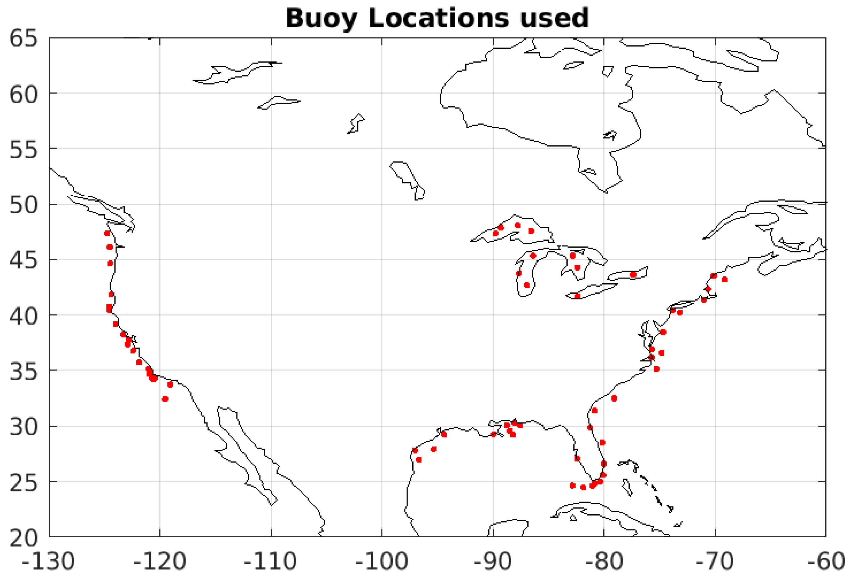
For validation we use National Data Buoy Center (NDBC) data—we use only buoys that are within 100 km of coastline. In Figure 1 we plot all the buoy locations used in the analysis presented in this paper. We use 178 NDBC buoys, and we have about 1.7 million matchups with version 4.1 of QuikSCAT, 1.46 million matchups for V3.1, and 1.4 million matchups for V3. Finally, we use the Liu and Tang model [31] to convert the buoy measurements to 10 meter equivalent neutral winds.
Table 1 lists all the versions of the QuikSCAT retrieved winds described in this paper. The newest version (4.1/LCRES) is the one in which coastal winds are retrieved using the method described in this paper (https://podaac.jpl.nasa.gov/dataset/QSCAT_LEVEL_2B_OWV_COMP_12_KUSST_LCRES_4.1, accessed on 9 March 2020).
3. Method
3.1. Previous Work in Field
Two approaches have been used by other authors to retrieve QuikSCAT winds closer to the coast. The first method is the Land Contribution Ratio (LCR) thresholding technique [32] by Owen and Long. The second is the empirical land mask technique (ELM) [33] by Vanhoff et al. The LCR technique makes use of a more accurate and computationally intensive estimate of the spatial response, of each measurement. Here b is the antenna polarization and is the antenna azimuth angle. The spatial extent of each measurement is roughly a 25 km by 8 km rectangular intersection with an ellipse as shown in the leftmost panel of Figure 2 above. The spatial response differs from the spatial extent in that it quantifies how much a particular point on the ground contributes to the measurements. Since values over land are typically more than an order of magnitude higher than those over ocean, even land outside the nominal spatial extent can adversely impact wind retrieval.
The LCR is the ratio between the integration of R over land and R over the entire surface of the Earth. In practice, everything outside a 100-km radius circle centered at the measurement centroid can be ignored, to speed things up. In [32], measurements with LCR exceeding a threshold were left out of wind retrieval. The threshold used was allowed to vary based upon local conditions. Land contamination is worst when the ocean is radar-dark (low wind speed) and the land is radar bright. Owen and Long used the largest nearby measurement over land and the lowest retrieved wind speed over nearby open ocean to set the LCR threshold to determine which measurements are omitted from each wind retrieval grid cell.
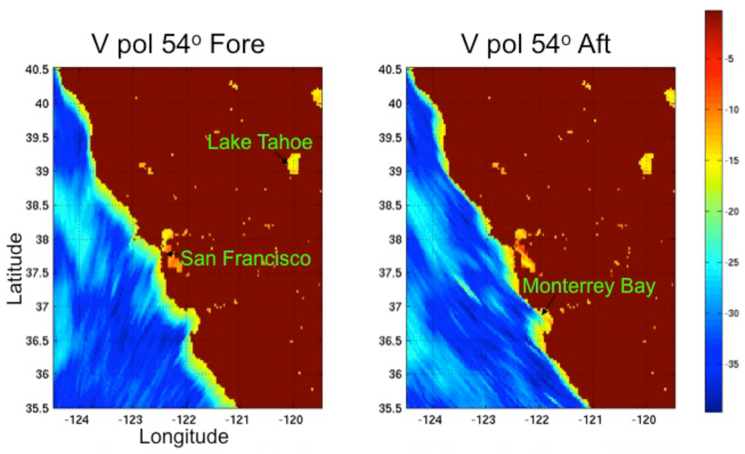
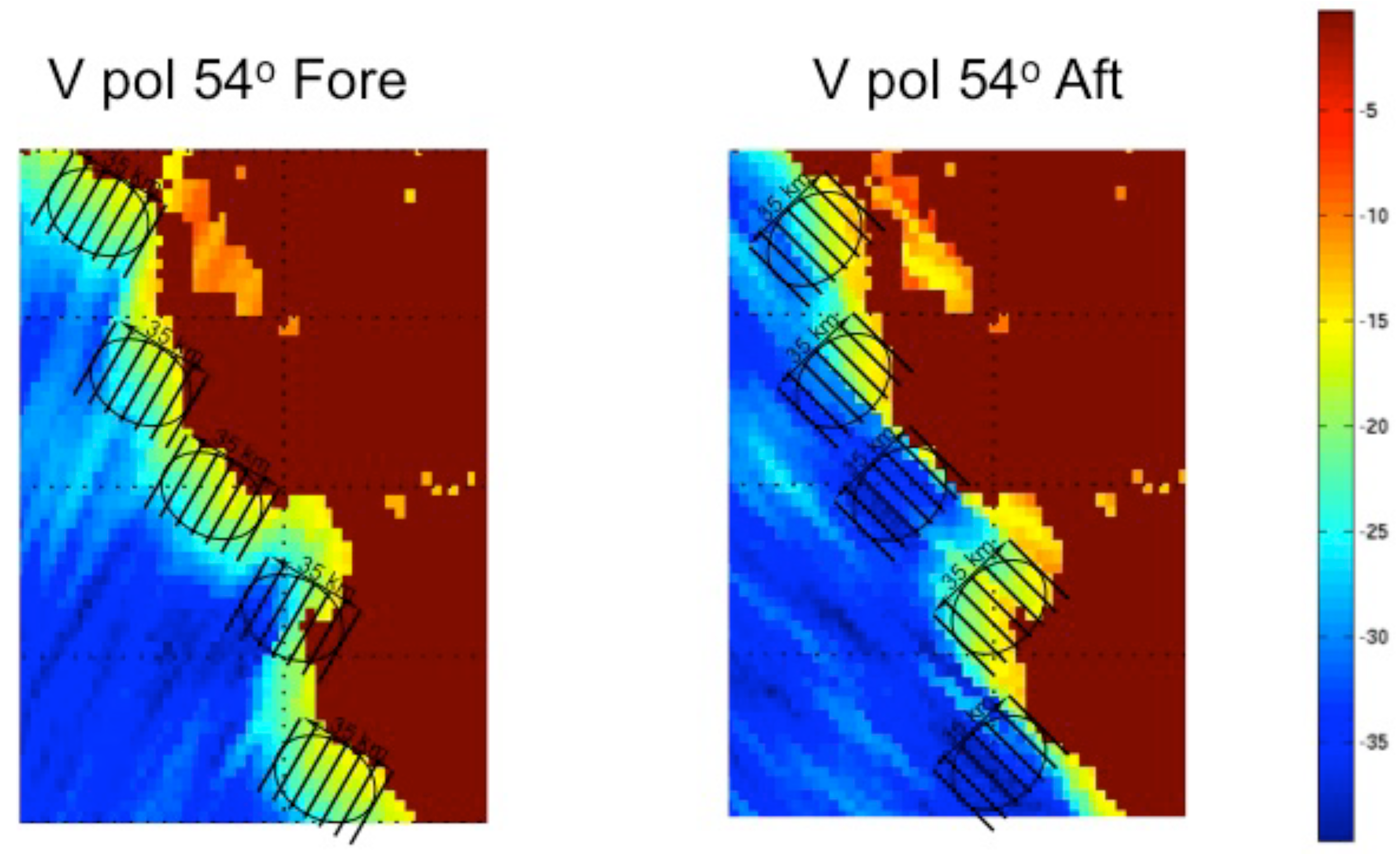
This is typically a conservative approach unless off-shore winds are higher than winds nearer the coast. The LCR approach allows measurements that are fortuitously oriented to get closer to the coast. Figure 3 demonstrates how land contamination varies for measurements from two different azimuth looks along the California coast. The radar-bright halo around the coast varies in thickness depending upon precisely how the measurements align with the coast. Figure 4 expands a portion of the coast and shows the approximate measurement shapes to illustrate the affect. When the slices are parallel to the coast the region of land contamination is thin. When they are perpendicular, the contaminated region is thick. Bays and peninsulas can complicate the situation. The ELM approach estimates a different land mask for each antenna beam and azimuth angle [33]. The land mask is determined based on the normalized standard deviation (standard deviation divided by the mean) of the measurement data. measurements over ocean have large variability because of the effect of wind speed on . measurements due to typical high winds (15 m/s) can be 20 or more times higher than those for typical low winds (3 m/s) and more extreme winds can vary even more. Over land however, values usually have much smaller variance when a single azimuth angle is considered (i.e., a factor or 1.5 or less between low and high extremes). Vanhoff et. al. created a set of land masks for each azimuth angle and antenna beam M(azimuth, beam, lat, lon) such that M was set to 1 if measurements with that centroid location (lat, lon), beam, and azimuth angle had variability less than a threshold value. M was set to 0 otherwise. The variabilities (and thus M) were computed using a long time sequence of measurements for each location, azimuth, and beam. During wind retrieval, these land masks were applied so that measurements in location and instrument geometry regimes with M = 1 were excluded from wind retrieval. The LCR and ELM techniques have complementary sources of error. ELM has the disadvantage that it is only as good as its assumption about variability. In rare instances where land is highly variable, ELM will mistake that land for ocean. In similar instances where wind does not vary much, ELM may mistake ocean for land. One must choose a cutoff for the variability level that is associated with land interference. The variance does not drop off as a step function as land is approached. Also, different locations and seasons have somewhat different shapes for the plot of variance as one approaches land. While LCR has fewer empirical assumptions, it relies on accurate measurement shape, location, and land maps. The strength of the ELM technique is that long term statistical errors in measurement location, are folded back into the land masks appropriately. Measurement location errors will automatically widen the regions in the land masks where M = 1. Unlike LCR, the ELM technique makes no use of the spatial response of each measurement or any a priori land map. ELM empirically generates a synthesis of measurement spatial response and land location from the data. So errors in our knowledge of the location of land or the spatial response of the measurement do not impact ELM.
3.2. Proposed Land Correction Technique—Land Contribution Ratio Expected
The proposed technique is a combination of the ELM and LCR methods, which we call LCRES. The first step in our method is to perform an LCR computation for every slice of QuikSCAT that is near a coastline, or the shore of a lake. We compute the LCR as
where the l superscript indicates land, is the spatial response function, which is a function of the spatial location (x,y), the antenna polarization b, and the antenna azimuth angle , and is the land map which is 1 over land and 0 otherwise. The land fraction, or LCR, value itself is quite useful for flagging and is the coastal data processing used for QuikSCAT version 3.1 data (https://podaac.jpl.nasa.gov/dataset/QSCAT_LEVEL_2B_OWV_COMP_12_LCR_3.1, accessed on 9 March 2022). The version 3.1 data is used for comparison in a later section. However, we can do better by combining the LCR value with the value over land to adaptively weight the land contamination values by the radar brightness of the land that is included in the spatial response of the radar slice . We compute , the expected contribution to from land, for a QuikSCAT slice as
where is the expected at location (x,y). We then use the value (henceforth referred to as ES) to flag slice as being contaminated by land, which allows for more strict flagging in locations where land is radar-dark, and less strict flagging in radar-bright areas. Finally, we remove the expected land contribution from to obtain an estimate of the water-only .
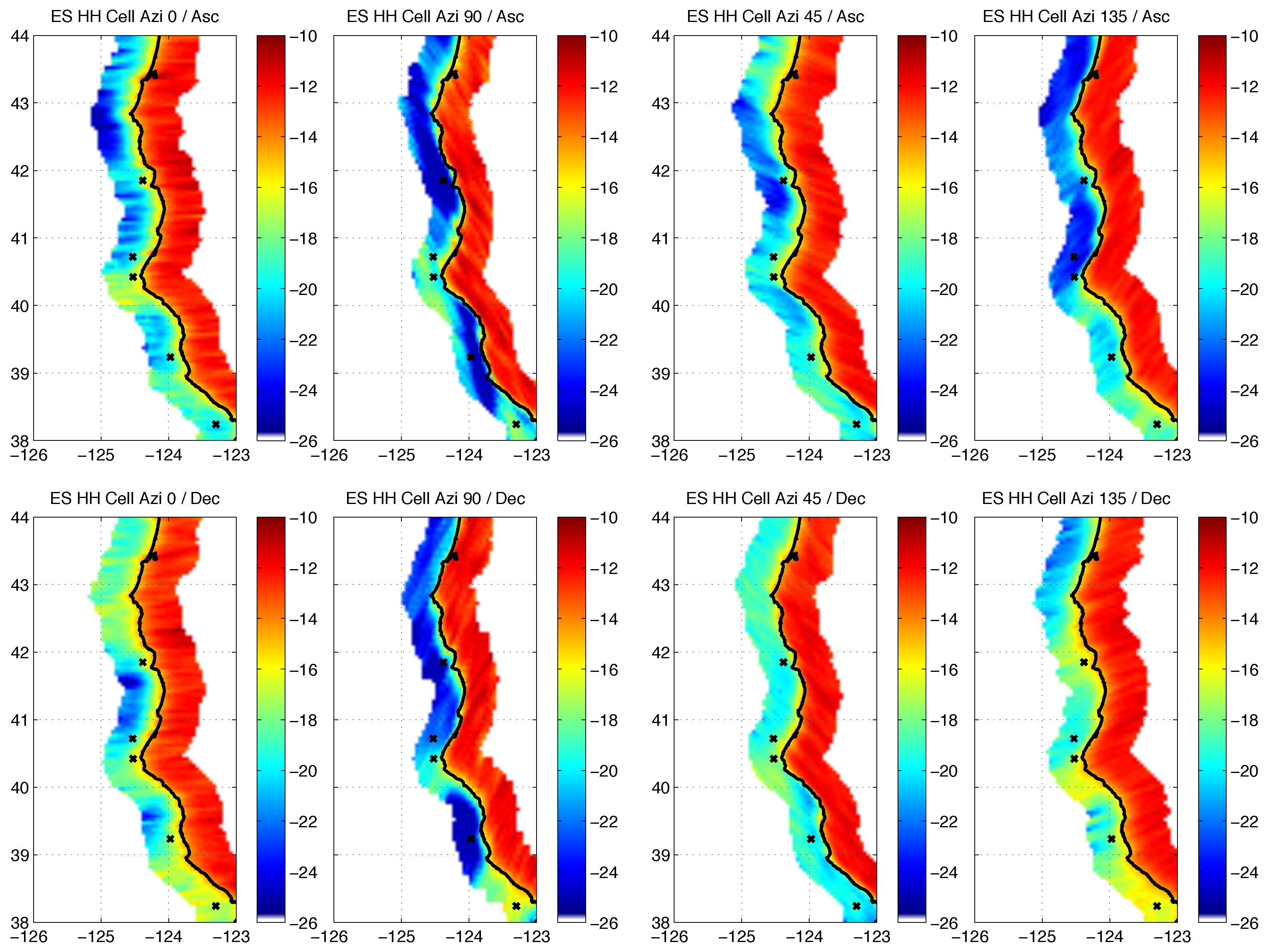
We have computed ES, as a lookup table , where are the latitude and longitude from the 10 years of QuikSCAT data itself. To do this we loop over all of the orbits of QuikSCAT, and for each slice we compute the total spatial response, as well as that only over land, and accumulate the the sum response over land times the slice , and the total response for all 10 years of QuikSCAT. We accumulate monthly maps of ES into a climatology that allows for seasonal variations that repeat each year. In Figure 5 we show ES for four different antenna azimuth angles off the western coast of the United States. The top row contains ES for HH polarization at 0°, 45°, 90°, and 135° antenna azimuth angle for ascending, and the bottom shows the same for descending. We can clearly see how much ES varies in the coastal region versus antenna azimuth angle and location, it is very important to account for the different viewing geometry as well as location.
Once we have computed the LCR value and have the climatology of ES we may compute the land-corrected as
where the super-script lc denotes land corrected, is the LCR, and is the ES from the look up tables. This equation may be derived by considering the total to be a linear combination of that from land, weighted by the land fraction, and that from water, weighted by one minus the land fraction.
4. Coastal Processing of QuikSCAT Slice to Coastal Wind Vectors
We have reprocessed the entire QuikSCAT data record, from 19 July 1999 to 21 November 2009—nearly 54,000 orbits of QuikSCAT data. The reprocessing begins with the version 2 L1B slice dataset and produces new version 4.1 netCDF data products. For every slice , first we check how close that slice is to the coast using an ancillary distance from nearest coast map (see Section 2); if it is within 50 km of nearest coast we continue with coastal processing, if not we use non-coastal processing. Next, for the coastal slices only, we integrate over the slice and compute the LCR value using the method discussed in Section 3. Once we have the LCR value we use the climatology of ES look-up tables to compute the LCRES value as the product of the LCR times the ES value. If that LCRES value for this slice is larger than we remove this slice from further wind processing; otherwise we apply Equation (3) to compute the corrected for that slice before wind retrieval. Finally, during wind retrieval we modify the maximum likelihood estimator (MLE) to use measured variance weighting instead of predicted variance. Using measured variance allows residual land contamination or land correction errors to be de-weighted in the MLE retrieval of ocean surface wind vectors from .
Data-Driven Quality Control and Flagging
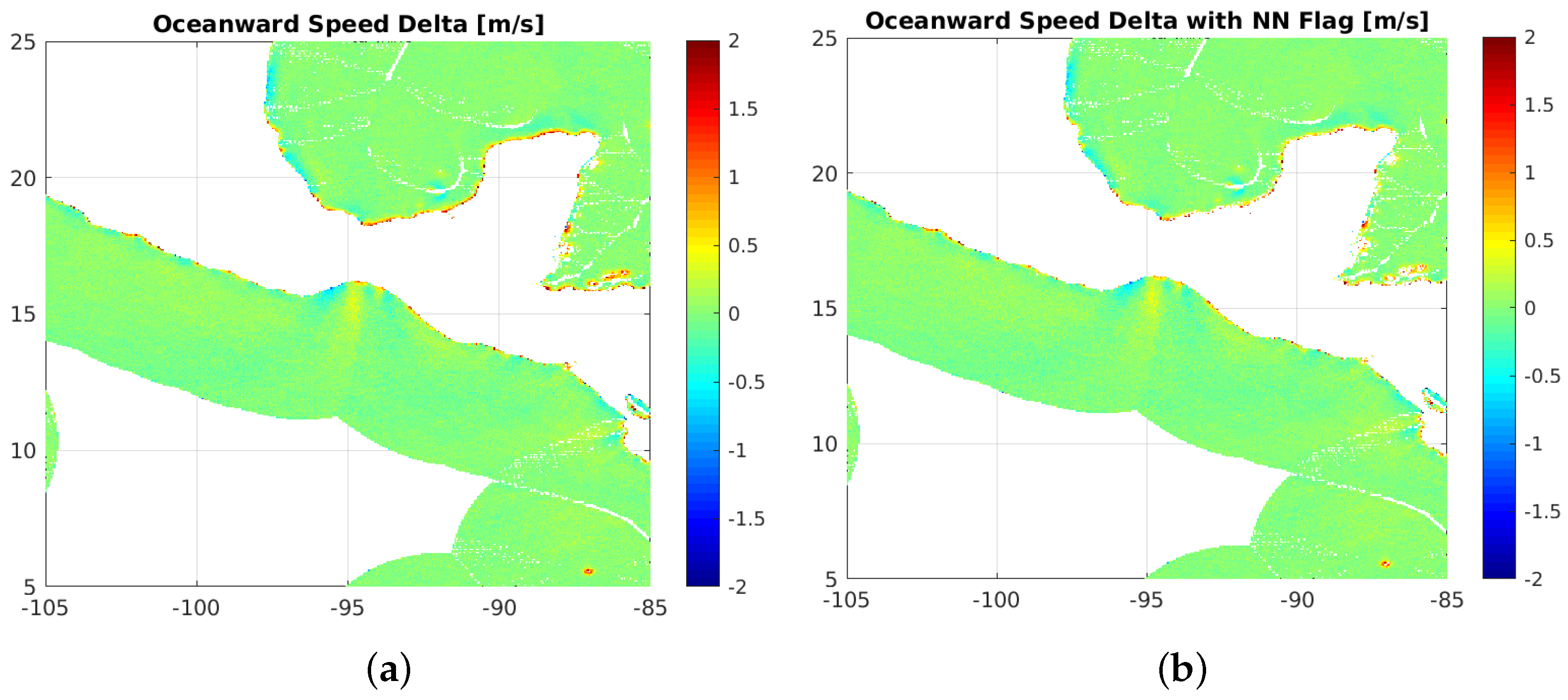
Having generated a coastal data set for the entire 10 years of QuikSCAT using the LCRES correction we have found some regions that have persistent residual land contamination, such as the region shown in Figure 6a. Here we show the mean oceanward wind speed difference, which is computed by comparing each WVC to its oceanward nearest neighbors, then averaging that difference into a map. We see that the northern shore has persistent land contamination that is not fully removed by the LCRES processing; however, the southern shoreline does not have the same issues. To address the residual land contamination left after LCRES processing of slice data, we have generated a neural network estimate of the oceanward wind speed bias as a function of the geographic means and standard deviations of QuikSCAT wind speeds retrieved with and without the LCRES correction. The neural network estimate is used as a flag instead of the oceanward speed bias itself in order to avoid erroneously flagging wind jets as poor retrievals. While wind jets do induce a bias with respect to oceanward neighbors, they do not exhibit a difference in the high spatial resolution inputs that the neural network uses to estimate those biases. In short, the neural network does not have access to the misleading information in the structure of the larger area wind field that compromises a flag using the oceanward bias itself. We flag the coastal data by applying a threshold of 0.4 m/s to the neural network generated map. Retrievals in locations on the map with values higher than the threshold are flagged as poor regions of coastal data processing. Additionally we flag all data within 5 km of land as having poor coastal processing. In Figure 6b.
5. Results
5.1. Buoy Comparisons
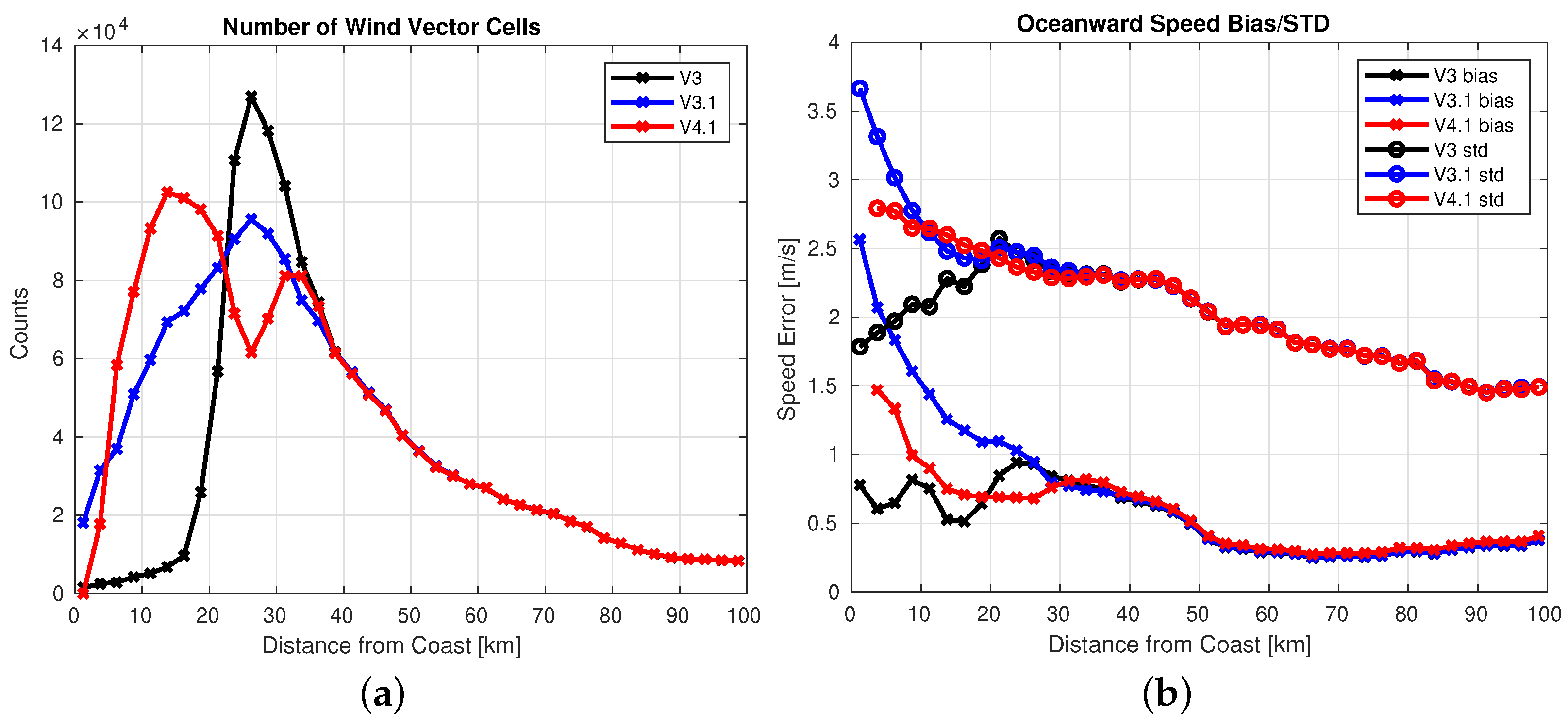
We have collocated the new QuikSCAT coastal product with NDBC buoys that are within 100-km of the coast; those buoy locations are shown in Figure 1. In Figure 7a we plot the number of buoy matchups as a function of distance to nearest coastline for versions 3 (no coastal processing), 3.1 (LCR processing), and 4.1 (LCRES processing) of QuikSCAT. In Figure 7b we show the speed bias and standard deviation (std) as compared to buoy wind speed as a function of distance from coastline. We see that with the LCRES method we have many more observations near the coast, as much as 10 times more within 20 km of coast. The V3 processing has very few WVCs closer to the coast than 22.5 km, while the V4.1 coastal processing gets as close to the coast as 10 km, and the V3.1 processing is somewhat closer to the coast than the V3 processing. The performance of these new WVCs in V4.1 closer to the coast than 22.5 km is nearly as good as the V3 product at 22.5 km; in particular we note that V4.1 lower wind speed bias between 10 km and 25 km and similar wind speed std except below 12 km or so from coast where it is slightly worse. All of the data show an increase in errors as compared to buoys as we approach the coast, however, that is not all due to land contamination as the V3 QuikSCAT product has a very conservative land control applied. Furthermore, spatial inhomogeneity in the coastal region complicates comparisons of the spatially-averaged wind estimate from scatterometers with the point source observations from buoys so this increase in errors is expected to some degree.
Note that the binning algorithm used in V3 and onwards over-samples the slice into the WVC grid which tends to cause noticeable ‘bunching’ effects near coastlines [1]. The inclusion of more coastal slices in version 4 and 3.1 explains the relative decrease of less-coastal WVCs (between 20–40 km from coast) and increase in more coastal WVCs (less than 20 km from coast) in the right plot of Figure 7.
5.2. Comparisons to Oceanward WVCs
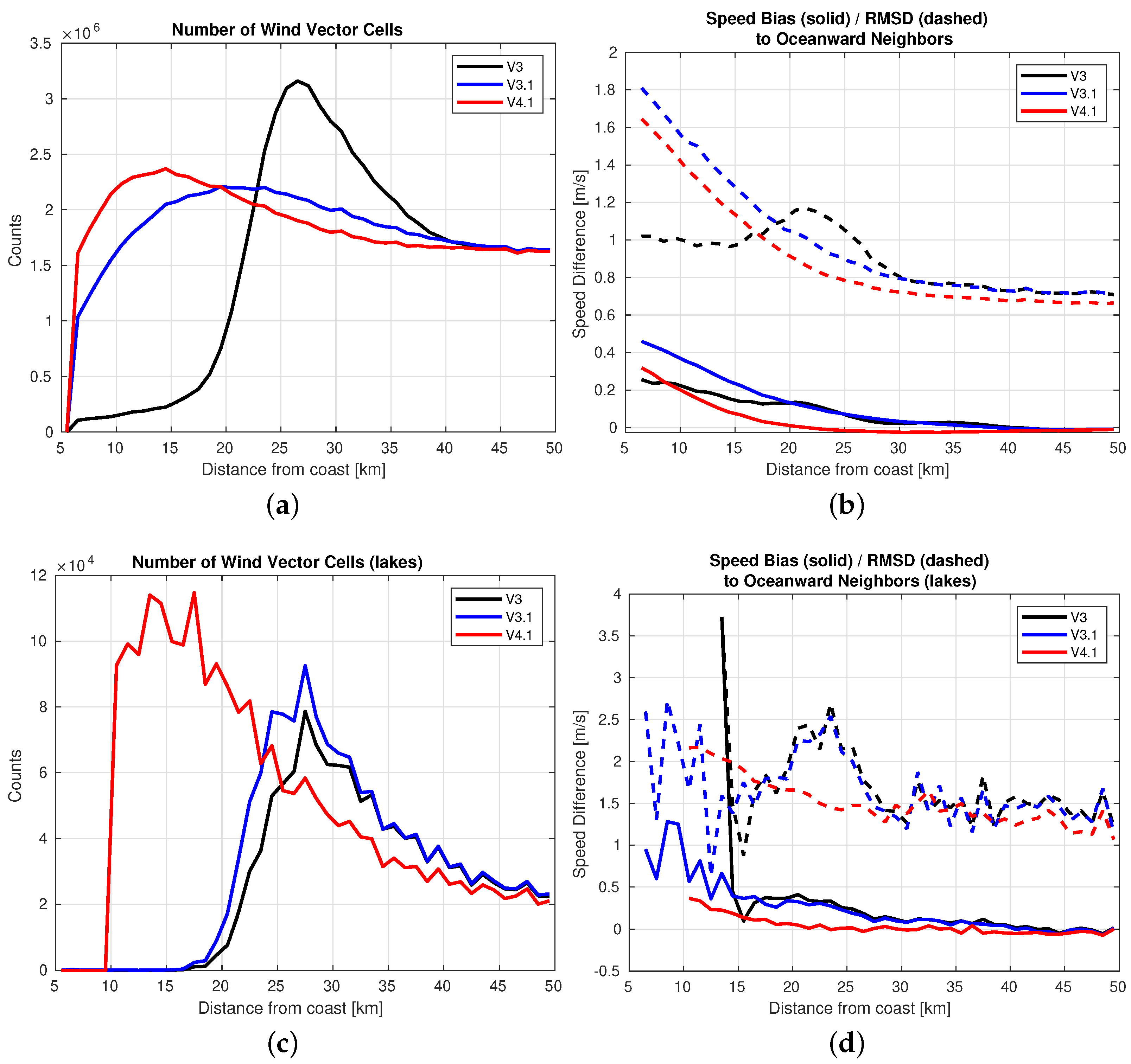
We also considered an alternative method of quantifying the coastal land contamination in a WVC: by comparison to the average of the adjacent WVCs (the adjacent WVCs are the eight nearest neighbors) which are further from the coast. This allows us to see incremental increases in land contamination as we get closer to the coast. In Figure 8 we compare each coastal WVC to the average of its nearest-neighbors which are further away from the coast, then we create statistics as a function of distance from coast. In Figure 8a we show the number of WVCs as a function of distance from coast over ocean, in Figure 8b we plot the speed bias and root-mean-square (RMS) difference as compared to oceanward neighbors, as a function of distance to coast. In Figure 8c,d we plot the same metrics, but over large inland lakes. Again, we first note that the V3 QuikSCAT has very little WVCs closer to the coast than 22.5 km, which has a conservative land rejection threshold. Over ocean, we note that the V3 product sharply drops off in counts around 22.5 km from coast, while V3.1 and V4.1 get much closer to the coast. Over lakes, we find V4.1 gets much closer to the coast than either V3 or V3.1, both of which get no closer than about 22.5 km, while V4.1 gets as close as 10 km to coast. The bias of the V4.1 products is better than that of the V3 and V3.1 products until under 10 km, while the RMS differences are better than V3 at 22.5 km until about 13 km from coast, then about m/s worse at 10 km, and m/s worse as it approaches the lower limit of 5 km from coast. Similarly, over lakes we see that V4.1 has less bias than V3 at 22.5 km while having smaller RMS differences. Note that the same effect is happening in these comparisons as in the buoy comparisons; that is, that the gridding algorithm used causes a bunching effect of the WVC centroids near coastlines, which explains the decrease in WVCs from about 20–40 km and increase below 20 km for the upper-left and lower-left plots in Figure 8.
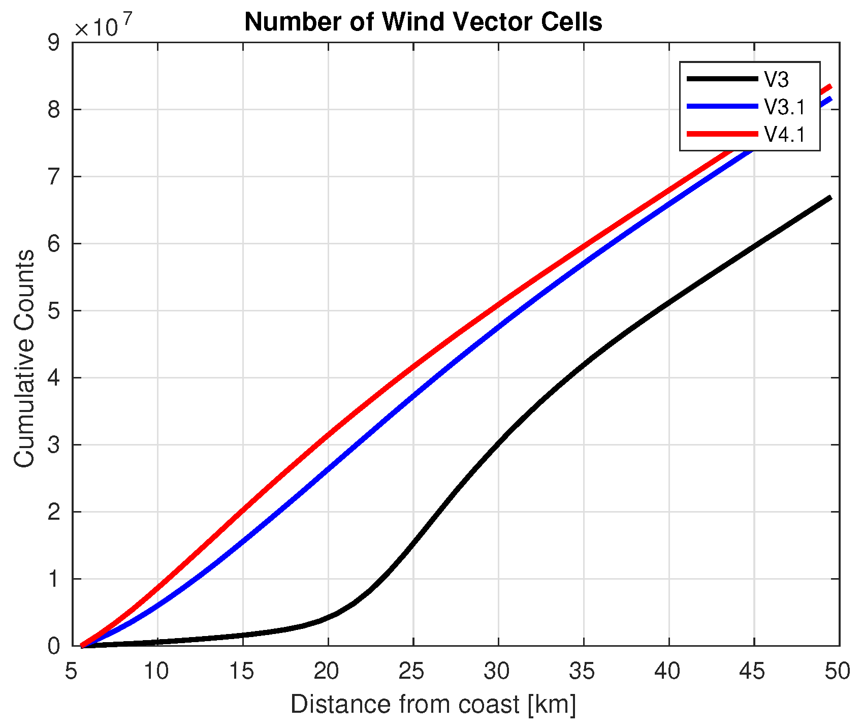
We can quantify the increase in coastal wind vector cells by looking at the cumulative counts ( total number of samples at a distance less than x from the coast) we show in Figure 9. We can see that there are nearly 10× as many wind vector cells within 20 km of coast in V4.1 as compared to version 3, and we are increasing the number of WVCs as compared to V3.1 even as we reduce the speed bias and STD as compared to oceanward neighbors.
6. Discussion and Conclusions
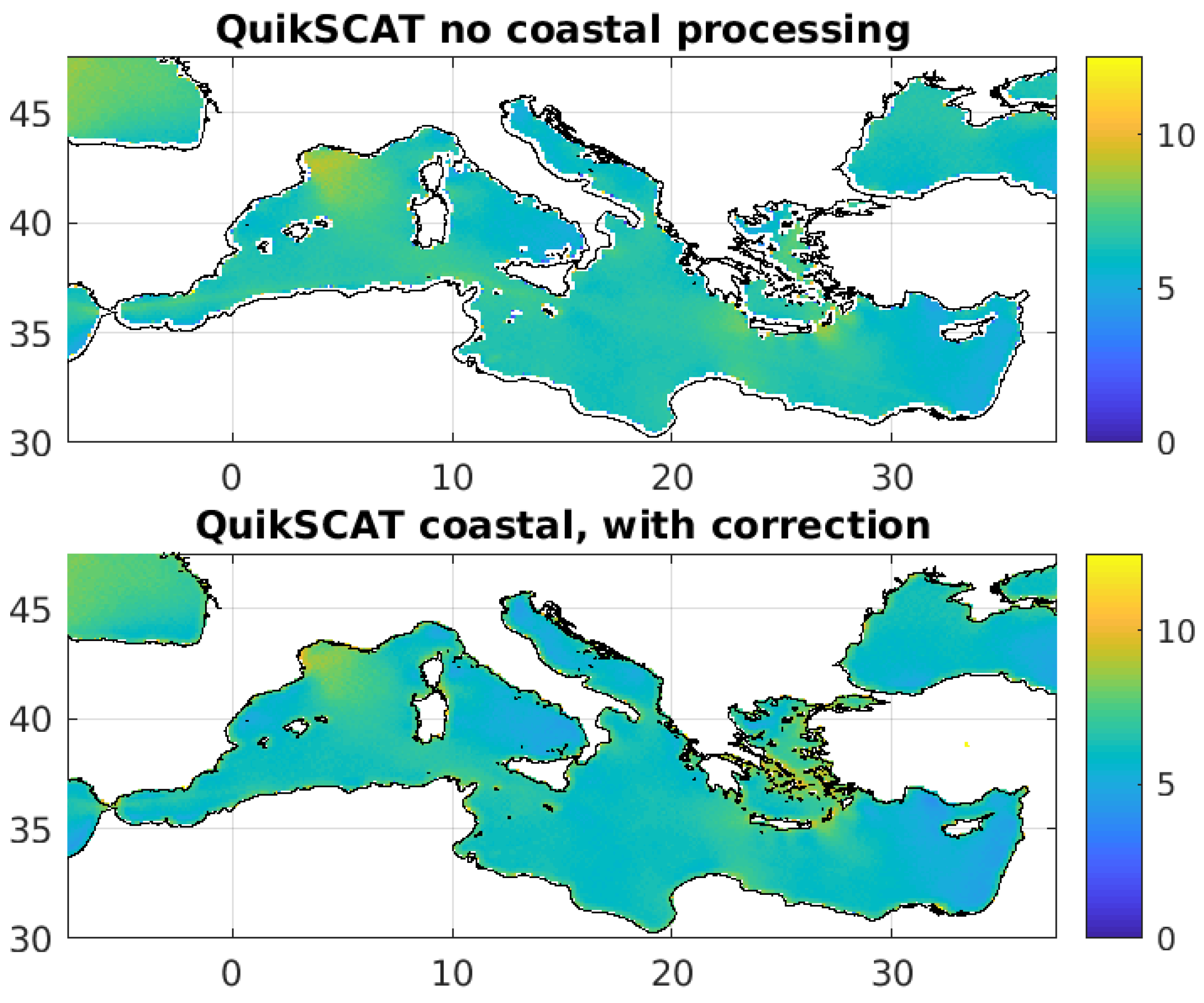
The QuikSCAT V4.1 with LCRES processing retrieves winds closer to the coast than ever before. We show that combining the LCR method with an expected significantly improves coastal ocean vector winds with QuikSCAT. We find nearly ten times more retrievals within 20 km of the coast, which are nearly the same quality as those of the V3 product at 22.5 km from coast as determined with comparisons to buoys and oceanward neighbors. There is a slight degradation between 5 to 10 km, which we mitigate using a data-driven neural-network based quality flag. The LCRES approach improved the version 4.1 data set as compared to the previous release (V3.1) by both removing residual land contamination and retrieving wind closer to the coast. Distance from the coast is also provided in the V4.1 product. In Figure 10 we show an example of QuikSCAT V4.1 compared to V3 over a region with significant land contamination, the Mediterranean Sea. We note a very significant increase in retrievals near to the coast where previously QuikSCAT had no data available.
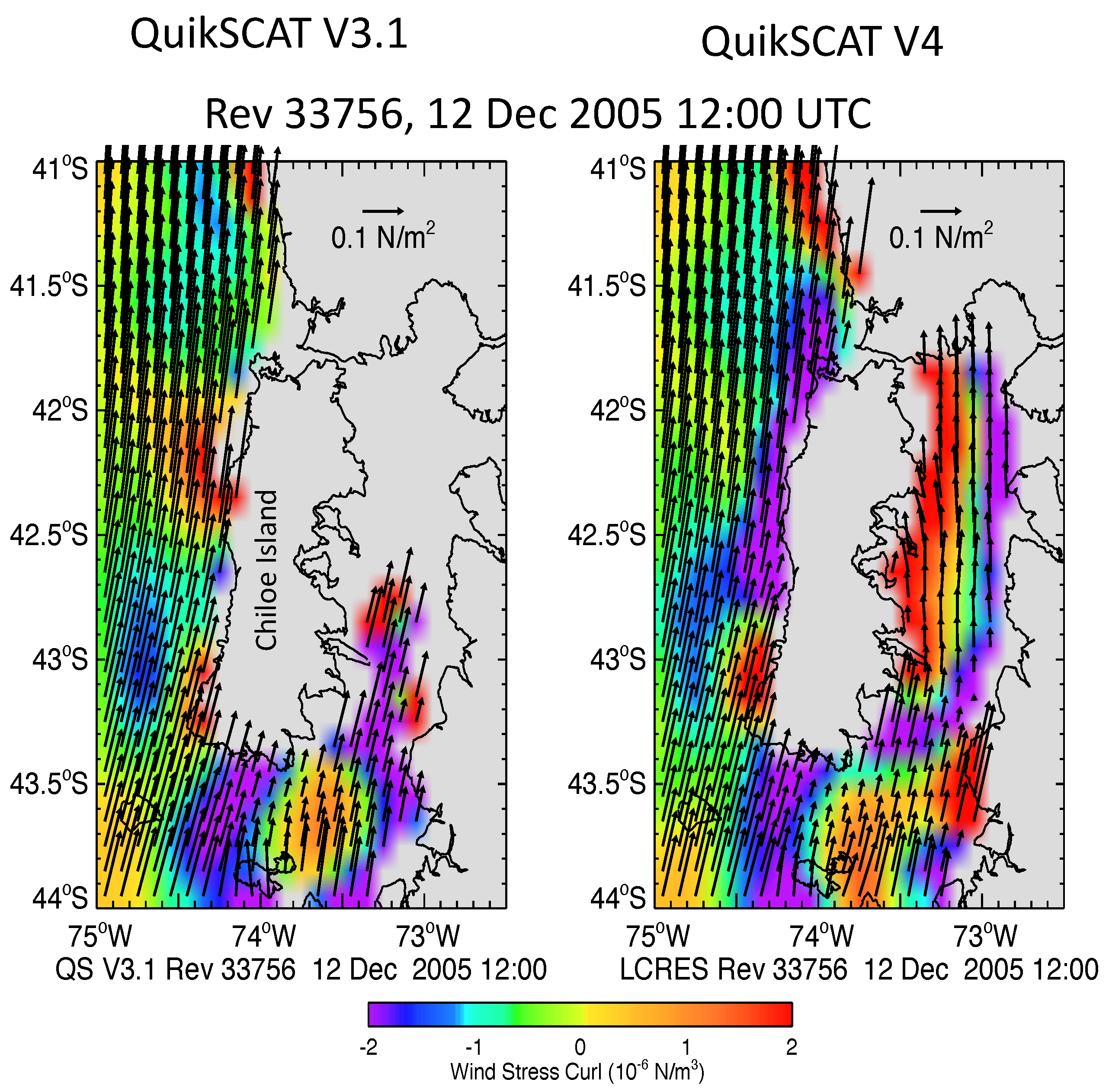
In the analysis of wind forcing of the ocean along southern Chile, Strub et al. [34] were only able to analyze coherent patterns of wind stress and wind stress curl along its west coast and within the inland sea inshore of Chile Island by using version 4.0 of the QuikSCAT processing, with LCRES correction for land contamination. In Figure 11 we show a image of the wind stress curl in this inland sea inshore of Chile island; on the left is the wind stress curl derived using QuikSCAT V3.1 data (with LCR based flag), and on the right is the same using QuikSCAT V4. Even the use of LCR data flagging in the earlier version 3.1 did not reveal realistic patterns of wind stress curl, which are necessary to understand the upwelling that drives high productivity of the marine ecosystem of this region. Globally, V4.1 has about 4% more WVCs with retrievals than V3 had. Finally, the version 4.1 winds are publicly available at https://podaac.jpl.nasa.gov/dataset/QSCAT_LEVEL_2B_OWV_COMP_12_KUSST_LCRES_4.1 (accessed on 16 May 2022).
Author Contributions
Conceptualization, B.W.S. and P.T.S.; Funding acquisition, B.W.S.; Investigation, A.G.F.; Methodology, A.G.F., B.W.S. and R.D.W.; Software, A.G.F.; Validation, P.T.S. and R.D.W.; Writing—original draft, A.G.F. and P.T.S.; Writing—review & editing, B.W.S. All authors have read and agreed to the published version of the manuscript.
Funding
The work reported here was performed at the Jet Propulsion Laboratory, California Institute of Technology, under contract with the National Aeronautics and Space Administration.
Data Availability Statement
Not applicable.
Conflicts of Interest
The authors declare no conflict of interest.
References
- Fore, A.; Stiles, B.; Chau, A.; Williams, B.; Dunbar, R.; Rodríguez, E. Point-Wise Wind Retrieval and Ambiguity Removal Improvements for the QuikSCAT Climatological Data Set. Geosci. Remote. Sens. IEEE Trans. 2014, 52, 51–59. [Google Scholar] [CrossRef]
- Perlin, N.; Skyllingstad, E.D.; Samelson, R.M.; Barbour, P.L. Numerical Simulation of Air–Sea Coupling during Coastal Upwelling. J. Phys. Oceanogr. 2007, 37, 2081–2093. [Google Scholar] [CrossRef] [Green Version]
- Haack, T.; Chelton, D.; Pullen, J.; Doyle, J.D.; Schlax, M. Summertime Influence of SST on Surface Wind Stress off the U.S. West Coast from the U.S. Navy COAMPS Model. J. Phys. Oceanogr. 2008, 38, 2414–2437. [Google Scholar] [CrossRef] [Green Version]
- Jin, X.; Dong, C.; Kurian, J.; McWilliams, J.C.; Chelton, D.B.; Li, Z. SST–Wind Interaction in Coastal Upwelling: Oceanic Simulation with Empirical Coupling. J. Phys. Oceanogr. 2009, 39, 2957–2970. [Google Scholar] [CrossRef] [Green Version]
- Gille, S.T.; Llewellyn Smith, S.G.; Statom, N.M. Global observations of the land breeze. Geophys. Res. Lett. 2005, 32. [Google Scholar] [CrossRef] [Green Version]
- Edwards, K.A.; Rogerson, A.M.; Winant, C.D.; Rogers, D.P. Adjustment of the Marine Atmospheric Boundary Layer to a Coastal Cape. J. Atmos. Sci. 2001, 58, 1511–1528. [Google Scholar] [CrossRef]
- Dorman, C.E.; Mejia, J.F.; Koračin, D. Impact of U.S. west coastline inhomogeneity and synoptic forcing on winds, wind stress, and wind stress curl during upwelling season. J. Geophys. Res. Ocean. 2013, 118, 4036–4051. [Google Scholar] [CrossRef]
- Winant, C.D.; Dorman, C.E.; Friehe, C.A.; Beardsley, R.C. The Marine Layer off Northern California: An Example of Supercritical Channel Flow. J. Atmos. Sci. 1988, 45, 3588–3605. [Google Scholar] [CrossRef] [Green Version]
- Enriquez, A.G.; Friehe, C.A. Effects of Wind Stress and Wind Stress Curl Variability on Coastal Upwelling. J. Phys. Oceanogr. 1995, 25, 1651–1671. [Google Scholar] [CrossRef] [Green Version]
- Bane, J.M.; Levine, M.D.; Samelson, R.M.; Haines, S.M.; Meaux, M.F.; Perlin, N.; Kosro, P.M.; Boyd, T. Atmospheric forcing of the Oregon coastal ocean during the 2001 upwelling season. J. Geophys. Res. Ocean. 2005, 110. [Google Scholar] [CrossRef] [Green Version]
- Chavanne, C.; Flament, P.; Lumpkin, R.; Dousset, B.; Bentamy, A. Scatterometer observations of wind variations induced by oceanic islands: Implications for wind-driven ocean circulation. Can. J. Remote Sens. 2002, 28, 466–474. [Google Scholar] [CrossRef]
- Dong, C.; McWilliams, J.C. A numerical study of island wakes in the Southern California Bight. Cont. Shelf Res. 2007, 27, 1233–1248. [Google Scholar] [CrossRef]
- Smith, R.B.; Grubišić, V. Aerial Observations of Hawaii’s Wake. J. Atmos. Sci. 1993, 50, 3728–3750. [Google Scholar] [CrossRef] [Green Version]
- Botsford, L.W.; Lawrence, C.A.; Dever, E.P.; Hastings, A.; Largier, J. Wind strength and biological productivity in upwelling systems: An idealized study. Fish. Oceanogr. 2003, 12, 245–259. [Google Scholar] [CrossRef]
- Wilkerson, F.P.; Lassiter, A.M.; Dugdale, R.C.; Marchi, A.; Hogue, V.E. The phytoplankton bloom response to wind events and upwelled nutrients during the CoOP WEST study. Deep Sea Res. Part II Top. Stud. Oceanogr. 2006, 53, 3023–3048. [Google Scholar] [CrossRef]
- Chavez, F.; Messié, M. A comparison of Eastern Boundary Upwelling Ecosystems. Prog. Oceanogr. 2009, 83, 80–96. [Google Scholar] [CrossRef]
- Barth, J.A.; Menge, B.A.; Lubchenco, J.; Chan, F.; Bane, J.M.; Kirincich, A.R.; McManus, M.A.; Nielsen, K.J.; Pierce, S.D.; Washburn, L. Delayed upwelling alters nearshore coastal ocean ecosystems in the northern California current. Proc. Natl. Acad. Sci. USA 2007, 104, 3719–3724. [Google Scholar] [CrossRef] [Green Version]
- LeMehaute, B.; Hanes, D.M. The Sea, Ocean Engineering Science; Wiley: Hoboken, NJ, USA, 1990; Volume 9, pp. 423–466. [Google Scholar]
- Brink, K.H.; Cowles, T.J. The Coastal Transition Zone program. J. Geophys. Res. Ocean. 1991, 96, 14637–14647. [Google Scholar] [CrossRef]
- Strub, P.T.; Combes, V.; Shillington, F.A.; Pizarro, O. Chapter 14—Currents and Processes along the Eastern Boundaries. In Ocean Circulation and Climate; Siedler, G., Griffies, S.M., Gould, J., Church, J.A., Eds.; Academic Press: Cambridge, MA, USA, 2013; Volume 103, pp. 339–384. [Google Scholar] [CrossRef]
- Aguirre, C.; Pizarro, Ó.; Strub, P.T.; Garreaud, R.; Barth, J.A. Seasonal dynamics of the near-surface alongshore flow off central Chile. J. Geophys. Res. Ocean. 2012, 117. [Google Scholar] [CrossRef] [Green Version]
- Strub, P.T.; Kosro, P.M.; Huyer, A. The nature of the cold filaments in the California Current system. J. Geophys. Res. Ocean. 1991, 96, 14743–14768. [Google Scholar] [CrossRef]
- Crawford, W.; Brickley, P.; Thomas, A. Mesoscale eddies dominate surface phytoplankton in northern Gulf of Alaska. Prog. Oceanogr. 2007, 75, 287–303. [Google Scholar] [CrossRef]
- Chelton, D.B.; Schlax, M.G.; Samelson, R.M. Global observations of nonlinear mesoscale eddies. Prog. Oceanogr. 2011, 91, 167–216. [Google Scholar] [CrossRef]
- Chelton, D.B.; Gaube, P.; Schlax, M.G.; Early, J.J.; Samelson, R.M. The Influence of Nonlinear Mesoscale Eddies on Near-Surface Oceanic Chlorophyll. Science 2011, 334, 328–332. [Google Scholar] [CrossRef] [PubMed]
- Gaube, P.; Chelton, D.B.; Strutton, P.G.; Behrenfeld, M.J. Satellite observations of chlorophyll, phytoplankton biomass, and Ekman pumping in nonlinear mesoscale eddies. J. Geophys. Res. Ocean. 2013, 118, 6349–6370. [Google Scholar] [CrossRef] [Green Version]
- Mann, K.H. Ecology of Coastal Waters: With Implications for Management; John Wiley & Sons: Hoboken, NJ, USA, 2000. [Google Scholar]
- Weiher, R.; Sen, A. Economic statistics for NOAA, 5th ed.; U.S. Department of Commerce: Washington, DC, USA, 2006. [Google Scholar]
- PICKETT, M.H.; SCHWING, F.B. Evaluating upwelling estimates off the west coasts of North and South America. Fish. Oceanogr. 2006, 15, 256–269. [Google Scholar] [CrossRef]
- Hasager, C.B.; Mouche, A.; Badger, M.; Bingöl, F.; Karagali, I.; Driesenaar, T.; Stoffelen, A.; Peña, A.; Longépé, N. Offshore wind climatology based on synergetic use of Envisat ASAR, ASCAT and QuikSCAT. Remote Sens. Environ. 2015, 156, 247–263. [Google Scholar] [CrossRef]
- Liu, T.; Tang, W. Equivalent Neutral Wind; Technical Report; JPL: Pasadena, CA, USA, 1996. [Google Scholar]
- Owen, M.; Long, D. Land-Contamination Compensation for QuikSCAT Near-Coastal Wind Retrieval. Geosci. Remote Sens. IEEE Trans. 2009, 47, 839–850. [Google Scholar] [CrossRef]
- Vanhoff, B.A.; Freilich, M.H.; Strub, T. QuikSCAT Level 3 Near-Coast Wind and Stress Fields with Enhanced Coastal Coverage (OSU): US West Coast Region; National Aeronautics and Space Administration: Washington, DC, USA, 2013. [Google Scholar]
- Strub, P.T.; James, C.; Montecino, V.; Rutllant, J.A.; Blanco, J.L. Ocean circulation along the southern Chile transition region (38°–46°S): Mean, seasonal and interannual variability, with a focus on 2014–2016. Prog. Oceanogr. 2019, 172, 159–198. [Google Scholar] [CrossRef]
Figure 1.
Locations of NDBC buoys used in this data analysis, we use all NDBC buoys that were within 100 km of coastline, including some in the Great Lakes.
Figure 1.
Locations of NDBC buoys used in this data analysis, we use all NDBC buoys that were within 100 km of coastline, including some in the Great Lakes.

Figure 2.
QuikSCAT Measurement Geometry. The geometry is shown on three scales. On the left, the smallest scale illustrates the spatial extent for the measurements (about 8 km by 25 km range slices) obtained during a single radar observation. Range slices are produced by breaking up the energy received by the radar into range-to-target bins. The middle panel shows multiple observations (footprints) obtained by the spinning antenna. The rightmost panel shows a portion of the pattern inscribed on the ground by the two rotating antenna beams. The blue circles are two rotations of the outer 54-degree incidence angle beam, and the red circles are rotations of the inner 46-degree incidence angle beam. The dots at the center of each circle are the location of the spacecraft in its orbit when that circle was inscribed. The black rectangle illustrates where measurements from four different azimuths (arrows) overlap. Measurements from different azimuths are required to retrieve wind direction and speed.

Figure 3.
Land contamination in raw data for low wind (≈5 m/s) conditions. Land contaminates and thus wind up to 30 km from the coast. How far from the coast it is contaminated depends upon the precise orientation of the measurements (range slices).
Figure 3.
Land contamination in raw data for low wind (≈5 m/s) conditions. Land contaminates and thus wind up to 30 km from the coast. How far from the coast it is contaminated depends upon the precise orientation of the measurements (range slices).

Figure 4.
As in Figure 3 with the region near Monterrey Bay expanded and the orientation of the range slices illustrated.
Figure 4.
As in Figure 3 with the region near Monterrey Bay expanded and the orientation of the range slices illustrated.

Figure 5.
Images of ES for the west coast of United States for December, January, and February 2008. We plot the ES for cell azimuths 0, 90, 45, and 135 (left to right) for ascending (top) and descending (bottom). The slices orientations depend on not only the cell azimuth angle but also ascending/descending since the slices are limited by frequency not range. This plot illustrates the highly variable slice ES as a function of cell azimuth, relative coastline orientation, and ascending/descending. The black x markers show the locations of buoys used in some of our coastal data analysis.

Figure 6.
(a) Map of average coastal wind speed bias as compared to that WVC’s oceanward neighbors. (b) Same with data flagged as poor coastal processing by this neural network removed. For each WVC we compute the speed bias versus its less coastal nearest neighbors, then accumulate that difference into this map. The less coastal nearest neighbors are the WVCs which are immediately adjacent to the WVC in question, which are also further from the coastline. We see that some regions have persistent errors, such as the northern shoreline in this sample image. We use a neural-network based flagging algorithm that removes these regions with persistent errors.

Figure 7.
(a) Number of buoy matchups as a function of distance to nearest coast in km for versions 3 (no coastal processing), 3.1 (LCR processing), and 4.1 (LCRES processing). (b) Mean buoy wind speed difference as a function of distance to nearest coast in km for the same data versions. Note that the new processing has many more observations near to coast than the V3 processing—at least 10 times as many buoy hits within 20 km of the coast. We also notice that agreement from 10 km is only marginally worse than at 40 km from shore, while performance at 5 km from coast is significantly degraded.

Figure 8.
(a) Number of WVCs as a function of distance to nearest coastline, for QuikSCAT V3, V3.1 with LCR, and V4.1 with LCRES. (b) Speed bias versus oceanward neighbors, as a function of distance from nearest coastline, for the same datasets. (c) Same as upper-left but statistics only computed over large inland lakes with respect to lakeward neighbors. (d) Same as upper-right but statistics only computed over large inland lakes. We see many more WVCs near to coast in the LCRES method of processing than in V3 QuikSCAT without any coastal processing, and an improvement as compared to using just the LCR method. On the lower-right plot we note that the performance degradation close to coast is minimal as we get close to the coast.

Figure 9.
Cumulative number of wind vector cells as a function of distance from coast.

Figure 10.
(top) One year of QuikSCAT V3 data over the Mediterranean Sea, which does not include any coastal processing or correction. (bottom) Same for QuikSCAT V4.1. Note the data gap around land is nearly closed, as we retrieve useable winds up to 10 km from land. Overall QuikSCAT V4.1 retrieves about 4 percent more WVCs than version 3 did.

Figure 11.
(left) Wind stress curl for QuikSCAT V3.1 over an inland sea inshore of Chile island. (right) same for QuikSCAT V4 data. V4 retrieves enough data to predict gridded fields of wind stress and wind stress curl over most of the inland sea. The coherent bands of wind stress curl next to the coasts are consistent with a decrease of the northward winds next to land. This effect increases upwelling in regions of negative curl.


Table 1.
QuikSCAT Data Versions.
| Version | Coastal Processing Method | Description |
|---|---|---|
| 3.0 | Conservative Flagging | 20 km distance threshold from low-res landmap. |
| 3.1 | Land Contamination Ratio | Reject slices with LCR value . |
| 4.0 | LCRES No QC | Same as 4.1 except no flag for poor coastal retrievals, not publicly available |
| 4.1 | LCRES | Reject slices with LCRES and use land correction. |
Publisher’s Note: MDPI stays neutral with regard to jurisdictional claims in published maps and institutional affiliations. |
© 2022 by the authors. Licensee MDPI, Basel, Switzerland. This article is an open access article distributed under the terms and conditions of the Creative Commons Attribution (CC BY) license (https://creativecommons.org/licenses/by/4.0/).
Share and Cite
MDPI and ACS Style
Fore, A.G.; Stiles, B.W.; Strub, P.T.; West, R.D. QuikSCAT Climatological Data Record: Land Contamination Flagging and Correction. Remote Sens. 2022, 14, 2487. https://0-doi-org.brum.beds.ac.uk/10.3390/rs14102487
AMA Style
Fore AG, Stiles BW, Strub PT, West RD. QuikSCAT Climatological Data Record: Land Contamination Flagging and Correction. Remote Sensing. 2022; 14(10):2487. https://0-doi-org.brum.beds.ac.uk/10.3390/rs14102487
Chicago/Turabian StyleFore, Alexander G., Bryan W. Stiles, Paul Ted Strub, and Richard D. West. 2022. "QuikSCAT Climatological Data Record: Land Contamination Flagging and Correction" Remote Sensing 14, no. 10: 2487. https://0-doi-org.brum.beds.ac.uk/10.3390/rs14102487
Note that from the first issue of 2016, this journal uses article numbers instead of page numbers. See further details here.