Prediction of Fine Particulate Matter Concentration near the Ground in North China from Multivariable Remote Sensing Data Based on MIV-BP Neural Network

Abstract

Rapid urbanization and industrialization lead to severe air pollution in China, threatening public health. However, it is challenging to understand the pollutants’ spatial distributions by relying on a network of ground-based monitoring instruments, considering the incomplete dataset. To predict the spatial distribution of fine-mode particulate matter (PM_2.5) pollution near the surface, we established models based on the back propagation (BP) neural network for PM_2.5 mass concentration in North China using remote sensing products. According to our predictions, PM_2.5 mass concentrations are affected by changes in surface reflectance and the dominant particle size for different seasons. The PM_2.5 mass concentration predicted by the seasonal model shows a similar spatial pattern (high in the east but low in the west) influenced by the terrain, but shows high value in winter and low in summer. Compared to the ground-based data, our predictions agree with the spatial distribution of PM_2.5 mass concentrations, with a mean bias of +17% in the North China Plain in 2017. Furthermore, the correlation coefficients (R) of the four seasons’ instantaneous measurements are always above 0.7, indicating that the seasonal models primarily improve the PM_2.5 mass concentration prediction.

1. Introduction

With the rapid development of the social economy in China, atmospheric particulate matter pollution is increasing each day. The fine particulate matter (PM_2.5) can directly reach and adhere to the human bronchus and lungs, even carrying a variety of germs, leading to cardiovascular and respiratory diseases, seriously affecting human health [1]. The Air Purification Act issued by the United Kingdom shows that PM_2.5 ranks fourth in major fatal factors in China [2]. Due to the long-term lack of ground monitoring network in China and the difficulty in obtaining PM_2.5 mass concentrations in a large range, domestic research on the long-term chronic health impact of PM_2.5 is very limited [3]. China also has serious PM_2.5 pollution, especially the North China Plain, which is far higher than the pollution level of Europe and the United States [4]. In recent years, the rapid industrialization, urbanization, and continuous consumption of fossil fuel in North China have led to the frequent occurrence of haze events [5].

Ground monitoring is the most direct way to obtain PM_2.5 concentrations. However, although data can be obtained through PM_2.5 ground monitoring stations after 2013, the incomplete coverage and uneven spatial distributions cannot reflect the PM_2.5 distribution of large regions [6]. The uneven distribution and the limited number of sites greatly reduce the accuracy of the data and cannot obtain comprehensive data in space. In the past 20 years, the aerosol optical depth (AOD) [7] product from satellite remote sensing used to estimate the temporal and spatial distribution of ground PM_2.5 concentration has become a promising technical means. Satellite remote sensing data have good spatial coverage and can provide large-scale, high-spatial resolution pollution distribution information, which has great advantages compared with that from ground PM_2.5 monitoring sites. A high correlation between AOD and PM_2.5 mass concentration was shown in the study by Zhi [8].

There are mainly four methods for estimating PM_2.5 mass concentration based on satellite remote sensing [9]. The first method is the univariate regression, which simply establishes the relationship between AOD and PM_2.5 [10,11]_. However, this relationship varies greatly in time and space, and is difficult to apply in practice. The second method is the empirical physical method. This method defines the volume extinction ratio to construct an estimation formula for PM_2.5 based on the physical mechanism [12]. This method has simple and flexible physical processes, and is more suitable for the processing of near real-time satellite observation. Zhang et al. [13] and Wei et al. [14] further updated the hygroscopic growth and mass conversion processes for this method, bringing a wider range of spatial applicability to this method. The third method is satellite remote sensing combined with a chemical transport model, usually referred to as CTM-Sat established by van Donkelaar et al. [15,16,17,18,19,20], who has made a great contribution in this field and improved it by assimilating various satellite observations, and then published a global dataset that provides basic data for health research. However, the CTM-Sat method also faces the problem of low accuracy in local heavily polluted areas. The fourth method involves statistical methods, such as the multiple regression method, this kind of model has relatively higher accuracy. These methods use a large amount of ground monitoring data to find out the relationship between different variables and PM_2.5 mass concentration through statistical methods, and then the PM_2.5 mass concentration can be predicted by the training models. However, due to the various compositions of PM_2.5 and various meteorological elements, the traditional statistical model method has certain limitations. In recent years, machine learning methods have shown strong nonlinear adaptability and have been widely used in the big data processing. Many scholars have tried to use machine learning algorithms to predict PM_2.5 mass concentrations. Hu et al. [21] established a PM_2.5 estimation model based on geographically weighted regression (GWR) using the AOD product from Moderate-resolution Imaging Spectroradiometer(MODIS), meteorological data from North American Land Data Assimilation System (NLDAS), and land cover data from as the predictor variables. This model can only fit a linear relationship for a certain location or time between surface PM_2.5 and the influencing variables, significantly inferior to geographically and temporally weighted neural network [22]. Li et al. [23] developed a PM_2.5 retrieval model using the random forest method, based on MODIS AOD data, near-ground meteorological data from the NASA Goddard Earth Observing System (GEOS). However, the development of structural changes of the random forest method is not as rich as artificial neural network (ANN). Since ANN have broader and more far-reaching applications than random forest and GWR, evaluating the performance of the most basic neural network, BP neural network, can provide a basis and benchmark for the improvement of complex neural networks. Therefore, this study uses the BP neural network to construct the PM estimation model.

In the above research, AOD at 550 nm is prevalent to predict the PM_2.5 mass concentrations, while other variables from remote sensing are ignored, such as AOD at other bands, fine-mode AOD, cloud reflection, and land reflectance. In order to better predict PM_2.5, we not only selected AOD variables, but also included the other 32 remote sensing variables in MOD04. Meanwhile, we evaluated the importance of these variables to the prediction of PM_2.5 using the mean impact value (MIV) method to filter the valid variables. Based on these analyses, a PM_2.5 predicting model is established by the back propagation (BP) neural network method. Combined with the ERA5 meteorological subdivision data of the European Centre for Medium-Range Weather Forecasts (ECMWF) and the PM_2.5 data of air quality monitoring stations, the annual near-surface PM_2.5 concentration was retrieved seasonally and a spatiotemporal analysis was conducted.

2. Study Area and Data

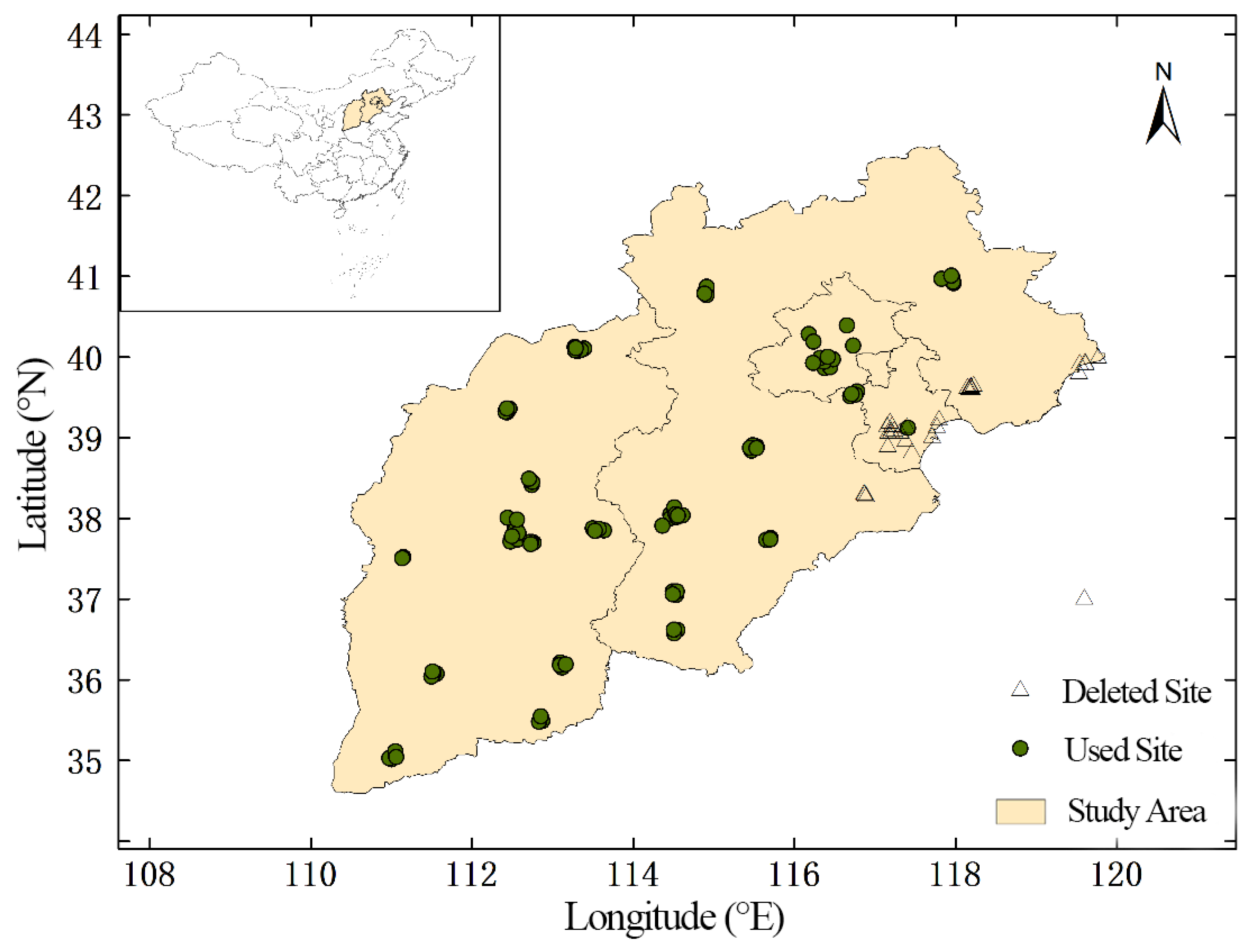
2.1. Study Area

In this study, four provinces (or cities) were selected as the study area in the North China region (109° E~120° E, 34° N~43° N, Figure 1), including Beijing, Tianjin, Hebei, and Shanxi. The topography of this area presents high in the northwest and low in the southeast due to the influence of two high mountains, the Taihang and the Yanshan. These areas have rapid economic development and relatively concentrated industries. Moreover, due to the rich mineral resources, the North China Plain is an important industrial base in China, and the industrial structure is also one of the important reasons for air pollution [24].

2.2. Data

The data used in this study include satellite remote sensing products, meteorological data, and ground-observed PM_2.5 mass concentration data. The remote sensing data from the MODIS C61 MOD04 AOD products from Terra satellite (https://ladsweb.modaps.eosdis.nasa.gov/search/ accessed on 20 September 2019). The spatial resolution of the products is 3 km, and the time range is from 1 January to 31 December 2017. Because the variables in MOD04 are directly or indirectly related to the AOD variables in MOD04, in order to analyze the influence of other variables on predicting PM_2.5, we did not only select a single AOD variable as other studies did, but included the remaining 32 remote sensing variables from MOD04. A comprehensive view of aerosol properties (multiwavelength retrieved AOD, aerosol types, fine mode AOD, corrected AOD), combined with the landcover features (multiwavelength surface reflectance data). These 32 remote sensing variables contained AOD inversed by other bands, AOD inversed by other algorithms, fine mode AOD, cloud reflection, and land reflectance. The meteorological data used in this study come from the ECMWF ERA5 hourly reanalysis dataset (https://cds.climate.copemicus.eu/cdsapp#!/dataset/reanalysis-era5-single-levels accessed on 10 March 2020), with a spatial resolution 0.25° × 0.25°. The main meteorological elements selected for the study include ground 2-m temperature, 2-m dew point temperature, total precipitation, surface pressure, boundary layer height, boundary layer dissipation, and 10-m wind field, in which the wind field data were divided into u-direction components and v-direction component. The hourly pollutant monitoring data were from 140 environmental ground stations in the Beijing–Tianjin–Hebei and Shanxi provinces from 1 January to 31 December 2017. These data were downloaded from the national urban air quality real-time release platform (http://106.37.208.233:20035/ accessed on 20 September 2019). The spatial distribution of monitoring sites is shown in Figure 1, using circle and triangle symbols. In the subsequent modeling process, low accuracy presents at some coastal sites, which may be relatively seriously affected by the oceanic boundary layer, thus not used in the model training.

3. Methods and Experiment Design

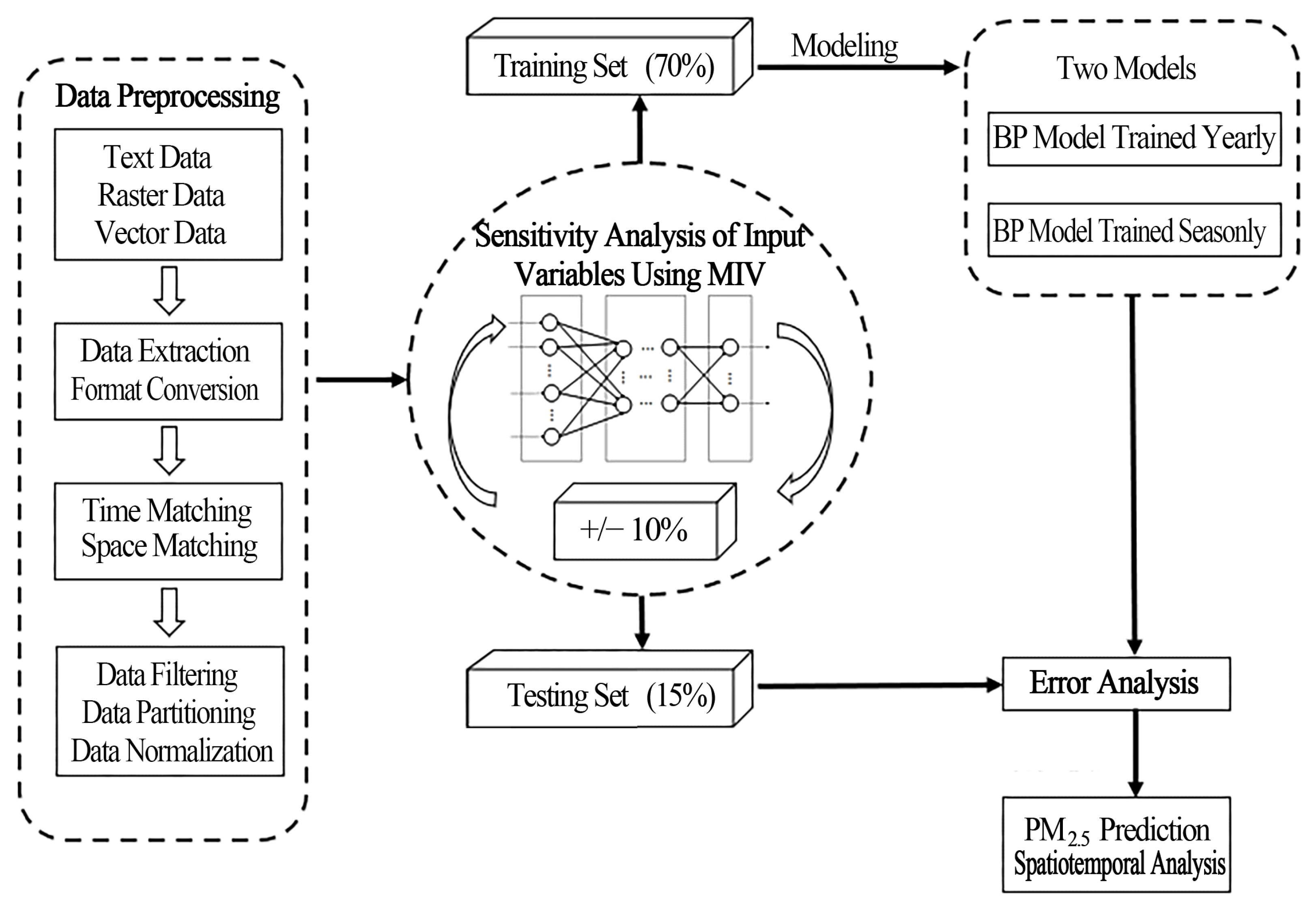
3.1. Data Preprocessing

Because there is a slight variation in the satellite transit time, and the spatial resolution of the satellite data are inconsistent with the ERA5 data, it is necessary to do space-time matching of the data. We take the mean value of surface PM_2.5 data at the observation sites within 2 h before and after the satellite transit times as the true PM_2.5 concentration. The ERA5 data were dealt with by bilinear interpolation to obtain the meteorological data at the site location. The satellite data at the monitoring sites were extracted to obtain the remote sensing parameters at the site location. The missing values of remote sensing data, meteorological data, and PM_2.5 observation data in the dataset were eliminated, and finally 15,056 samples were obtained.

3.2. MIV Algorithm to Analyze Remote Sensing Variables

This study uses the mean impact value (MIV) as an indicator to evaluate the importance of each input variable on the output variable. MIV is an indicator used to identify the influence of input neurons on output neurons. Its value represents the relative importance of the influence. The specific implementation process is as follows:

(1)

After completing the BP neural network training, respectively add or subtract 10% of each variable in the training sample to form two new training samples;

(2)

Take them as simulation samples, respectively, and use the established network to carry out simulations and obtain two simulation results;

(3)

Calculate the difference between these two simulation results, and the obtained value is the impact value (IV) of the impact of the input variable change on the output;

(4)

Calculate the average value of the impact value (IV) of all samples, and then the mean impact value (MIV) corresponding to this input variable can be obtained;

(5)

Repeat the above steps, and calculate the MIV value of each variable in turn;

(6)

Sort the calculated MIV values of each variable to obtain the influence weight of each input parameter on the prediction result.

According to the above method, the MIV value is calculated for each variable of the network input parameters, and the results are shown in

Table A1. Remote sensing variable information and MIV evaluation result table.

Variable Number	Variable	Description	Relative Contribution Rate (Full Year)/%
1	time	Day of the year	0.73
2	longitude	Longitude	15.86
3	latitude	Latitude	8.19
4	Land_Ocean_Quality_Flag	Quality flag for land and ocean Aerosol retrievals	4.48
5	Land_sea_Flag	Land_sea_Flag	4.37
6	Optical_Depth_Land_And_Ocean	AOT at 0.55 μm for both ocean and land	17.85
7	Image_Optical_Depth_Land_And_Ocean	AOT at 0.55 μm for both ocean and land with all quality data	15.23
8	Aerosol_Type_Land	Aerosol type	8.25
9	Fitting_Error_Land	Spectral fitting error for inversion over land	9.28
10–12	Corrected_Optical_Depth_Land 0.47, 0.55, 0.66 μm	Retrieved AOT at 0.47, 0.55, 0.66 μm	13.36, 15.69, 16.37
13	Corrected_Optical_Depth_Land_wav2p1 2.13 μm	Retrieved AOT at 2.13 μm	16.75
14	Optical_Depth_Ratio_Small_Land	Fraction of AOT contributed by fine dominated model	15.38
15–16	Number_Pixels_Used_Land 0.47 and 0.66μm	Number of pixels used for land retrieval at 0.47 and 0.66 μm	2.25, 3.91
17–23	Mean_Reflectance_Land 0.47, 0.55, 0.65, 0.86, 1.24, 1.63, 2.11μm	Mean reflectance of pixels used for land retrieval at 0.47, 0.55, 0.65, 0.86, 1.24, 1.63, 2.11 μm	4.23, 3.61, 2.64, 6.12, 6.46, 4.84, 4.51
24–30	STD_Reflectance_Land 0.47, 0.55, 0.65, 0.86, 1.24, 1.63, 2.11μm	Standard deviation of reflectance of pixels used for land retrieval at 0.47, 0.55, 0.65, 0.86, 1.24, 1.63, 2.11 μm	8.48, 6.20, 4.67, 4.65, 6.61, 7.29, 5.08
31	Mass_Concentration_Land	Estimated column mass (per area) using assumed mass extinction efficiency	4.26
32	Aerosol_Cloud_Fraction_Land	Cloud fraction from land aerosol cloud mask from retrieved and overcast pixels not including cirrus mask	19.64
33–35	Quality_Assurance_Land	Runtime QA flags	4.70, 9.99, 15.04
36	10 m wind field (u)	10 m wind field (u)	6.54
37	10 m wind field (v)	10 m wind field (v)	6.93
38	2 m dew point temperature	2 m dew point temperature	5.97
39	2 m temperature	2 m temperature	3.85
40	boundary layer dissipation	Boundary layer dissipation	0.02
41	Boundary layer height	Boundary layer height	1.10
42	surface pressure	Surface pressure	0.07
43	total precipitation	Total precipitation	6.56

.

3.3. Network Construction

The BP neural network is a feedforward network where information flows from input to output. It is based on error back-propagation. When the prediction error exceeds a certain value, according to the prediction error, back-propagation continuously adjusts the parameters of the network to be closer to the expected output [25]. Each iteration of BP neural network algorithm includes two processes, forward and reverse calculation process [26]. In forward calculation, the data are weighted and summed, and through the activation function, the data are transmitted forward, layer-by-layer, to obtain the output. The reverse calculation is used to update the parameters. When the error performance function cannot reach the expected value, the gradient descent method will be used to gradually correct the weight bias of the output layer and the hidden layer in reverse to reduce the error.

Assuming that the input layer, the hidden layer and the output layer have n, m, and s neurons, respectively, the input–output relationship of each layer is shown in Formulas (1)–(3):

$$\mathrm{Input}\mathrm{layer}:X_i=x_i\begin{array}{ccc}& & i=1,2,\dots ,n\end{array}$$

(1)

$$\mathrm{Hidden}\mathrm{layer}:A_j=f\left({\displaystyle \sum }_{i=1}^n{w}_{ij}{X}_i+b_j\right)\begin{array}{ccc}& & j=1,2,\dots ,m\end{array}$$

(2)

$$\mathrm{Output}\mathrm{layer}:O_k=g\left({\displaystyle \sum }_{j=1}^m{w}_{kj}{A}_j+b_k\right)\begin{array}{ccc}& & k=1,2,\dots ,s\end{array}$$

(3)

where x is the input variable, w is the connection weight, b is the bias, and f is the activation function, such as Sigmoid, TanH, and ReLU; g is the linear transfer function.

In the weight update stage, in order to minimize the value of the error performance function E_k, the gradient descent algorithm can be used to gradually correct the value of the connection weight and bias between the output layer and the hidden layer. The update of the error performance function and the weight of each layer is shown in Formula (4)–(6):

$$\mathrm{Error}\mathrm{performance}\mathrm{function}:E_k=\frac{1}{2}{\left(O_k-Y_k\right)}^2$$

(4)

$$\mathrm{output}\mathrm{layer}:d=\left(Y_k-O_k\right)g^{’}\left(w_{kj}\right),w_{k{j}_{new}}=w_{kj}+{\eta }_{1}d{A}_j$$

(5)

$$\mathrm{Hidden}\mathrm{layer}:h={\displaystyle \sum }_{k=0}^{s}d{w}_{kj}{f}^{’}\left(w_{ji}\right),w_{j{i}_{new}}=w_{ji}+{\eta }_{2}h{x}_i$$

(6)

Y is the true value, d and h represent the gradient term of the neuron, respectively, and η₁ and η₂ are the learning rates. The update step for biases is similar to that for weights.

After many experiments, the settings of the fully connected BP neural network used in this study are as follows: the activation function of the hidden layer adopts the hyperbolic tangent s-shaped activation function tanh; the transfer function of the output layer adopts the linear activation function; the optimization method adopts the Levenberg–Marquardt algorithm; the hidden layer is set to 18 layers; the learning rate is 0.01; the validity check is set to 10 times; the maximum number of iterations is 1000 times; the initial weight is random.

3.4. Experiment Design

The processed data are randomly divided into training set, validation set, and testing set according to the ratio of 7:1.5:1.5. We normalized each input variable to eliminate the dimensional difference, add/subtracted 10% of itself, and obtained the absolute value of MIV for 43 variables to analyze it. Depending on whether or not seasonal factors were considered, different forecasting models were trained. Then we determined the quality of the model by calculating the mean absolute error (MAE) and root mean square error (RMSE) of the real and predicted values. The optimal model was selected to predict the PM_2.5 concentration in Beijing–Tianjin–Hebei–Shanxi, and the spatiotemporal analysis was carried out. The technical route is shown in Figure 2.

The changes in PM_2.5 mass concentration tend to have strong seasonality as the weather conditions, underlying surfaces, and pollution sources change. So, three groups of models were designed for comparison when constructing the AOD-PM_2.5 model. The input of Group 1 were pure data of the whole year without the seasonal flag. The input of Group 2 was based on Group 1, adding a seasonal flag variable to enhance the sensitivity to the season, specifically: spring (March, April, May) marked with 1, summer (June, July, August) marked with 2, autumn (September, October, November) marked with 3, and winter (December, January, February) marked with 4. Group 3 trained the model for the four seasons, respectively. All settings were held fixed but the dataset was randomly assigned and trained again. One must repeat the above operations 30 times to eliminate the difference caused by the randomness of model training

4. Results

4.1. MIV of Input Variables

In this study, the MIV of AOD and 42 other remote sensing variables, such as the fine-mode AOD and cloud fractions from satellite products, were all analyzed.

Table 1. The most influential variable per season.

No.	Spring	Summer	Autumn	Winter
1	Corrected_Optical_Depth_Land_wav2p1 2.13 μm (6.79%)	Optical_Depth_Land_And_Ocean 0.55 μm (4.62%)	Corrected_Optical_Depth_Land_wav2p1 2.13 μm (4.65%)	Optical_Depth_Ratio_Small_Land (5.15%)
2	Aerosol_Cloud_Fraction_Land (6.70%)	Corrected_Optical_Depth_Land 0.47 μm (4.38%)	Aerosol_Cloud_Fraction_Land (4.62%)	Longitude (5.13%)
3	Optical_Depth_Land_And_Ocean 0.55 μm (6.51%)	Longitude (4.36%)	Corrected_Optical_Depth_Land 0.66 μm (4.53%)	Quality_Assurance_Land (4.89%)
4	Quality_Assurance_Land (4.83%)	Aerosol_Type_Land (4.28%)	Quality_Assurance_Land (4.42%)	Corrected_Optical_Depth_Land 0.47 μm (4.74%)
5	Corrected_Optical_Depth_Land 0.66 μm (4.38%)	Image_Optical_Depth_Land_And_Ocean 0.55 μm (4.17%)	Corrected_Optical_Depth_Land 0.55 μm (4.25%)	Image_Optical_Depth_Land_And_Ocean 0.55 μm (4.37%)

lists the MIVs of the most influential variables for the four seasonal models. Among the remote sensing variables, the PM_2.5 mass concentration in spring and autumn was most affected by the variable called Corrected_Optical_Depth_Land_wav2p1, more correlated with the AOD at 2.13 μm. The fine mode fraction in spring was lower than other seasons as shown in Figure A1. This is also related to the dust storm events [27] because the scattering and absorption for large aerosol particles can also affect the satellite observation at 2.13 μm, which means large AOD at 2.13 μm, unlike fine particles. Moreover, it can be explained by the surface reflectance changes due to vegetation growth cycles. The summer PM_2.5 mass concentration is most affected by the variable called Optical_Depth_Land_And_Ocean, which is more correlated with the AOD at 0.55 μm. In summer, the surface characteristics are stable and fine-mode particles dominate, so the total AOD can better represent PM_2.5 mass concentration, which is consistent with previous studies [28]. The PM_2.5 mass concentration in winter is most affected by the variable called Optical_Depth_Ratio_Small_Land, which is the fine mode optical thickness. This is because the total AOD can be affected by the coarse particles, such as dust events in the winter in northern China, fine-mode AOD can better characterize the pollution events related to fine particles. Moreover, the influence of longitude is greater than latitude in spring, autumn, and winter, indicating that the gap between the longitudes of PM_2.5 is larger, which is due to the blocking effect of the Taihang Mountains, which run north and south. However, there is no significant difference in the influence of latitude and longitude in the summer, indicating that the distribution of PM_2.5 in the summer is even. The sums of each variable MIV for the four seasonal models are shown in Table A1, listed from strong to weak.

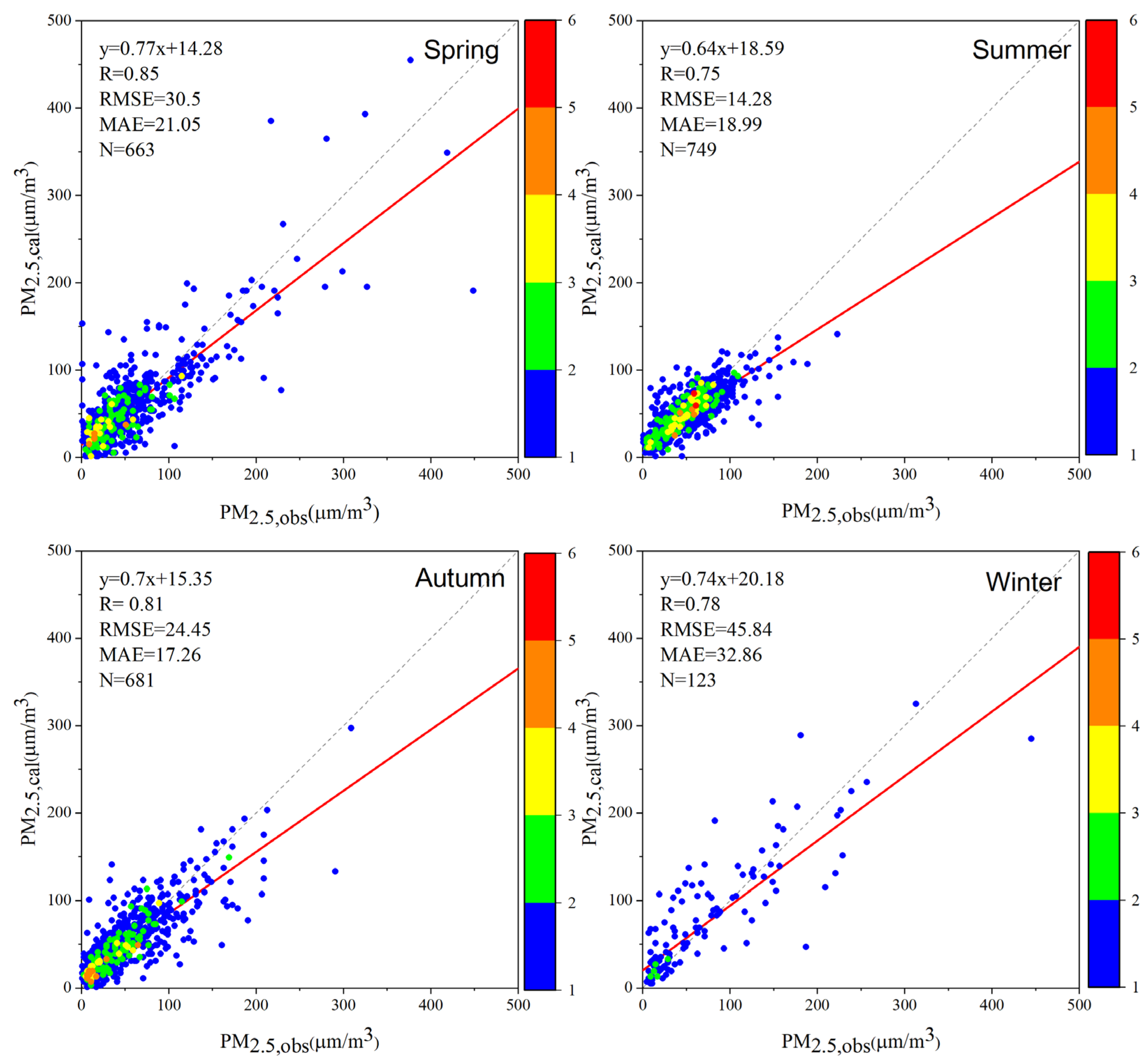
4.2. Evaluation of PM_2.5 Models

The fitting performance of each group of models on the testing set is shown in

Table 2. Comparison of the prediction performance of the three groups of models on the test set.

Which Group	MAE	RMSE	R
Group 1	21.5	32.19	0.70
Group 2	20.55	29.46	0.72
Group 3_Spring	21.05	30.50	0.85
Group 3_Summer	18.99	14.28	0.75
Group 3_Autumn	17.26	24.45	0.81
Group 3_Winter	32.86	45.84	0.78

. Comparing Groups 1 and 2, it can be seen that the indicators of Group 2 with the seasonal flag are better than that of Group 1, but the improvement is not significant. The improved fitting performance after adding the seasonal flag reflects the importance of PM_2.5 seasonality.

From the comparison of the seasonal models in Group 3, the indicators of MAE and RMSE show a trend, i.e., summer < autumn < spring < winter, and correlation coefficient R has a different trend, i.e., spring > autumn > winter > summer. It is indicated that although the fitting bias in summer is small and the data are more concentrated, the fitting correlation is low. There is a big difference between summer and winter in MAE and RMSE. The indicators besides R in winter are more than twice as high as those in summer, the fitted value and expected output value in winter are relatively scattered. The difference in R between spring and summer shows that the model performance is good in the spring and slightly less in the summer. From the comparison of the fitting performance of the three groups, the changes of PM_2.5 mass concentration has a strong seasonality, which needs seasonal modeling. For the seasonal models, the winter model has the worst evaluation indicators because of the lack of available data in this season. Compared with Groups 1, 2, and 3, the difference in R is not obvious.

In order to further compare the fitting and prediction ability of the four seasonal models, the scatter points with the predicted and observed values in the testing set for four seasons are displayed in Figure 3. It can be seen that the predictions of the models are quite different. Overall, the correlation coefficient R of the four seasons is above 0.7. The R between the observed and estimated values in spring reaches 0.85, which is the best in the four seasons. However, the RMSE reaches 30.5 μg/m³ in the spring, which is related to the high PM_2.5 mass concentration in the spring. In the summer and autumn, predictions for low values are better, while predictions for high values usually underestimate and have some errors. In the winter, the distribution of the scatter points of predicted and observed value has relatively large discreteness, but the correlation coefficient remains at 0.78. The RMSE in the winter reaches 45.84 μg/m³, because there is ice and snow on the surface in the winter, and MODIS has great uncertainty for the highlighted surface, so the prediction error is larger than other seasons.

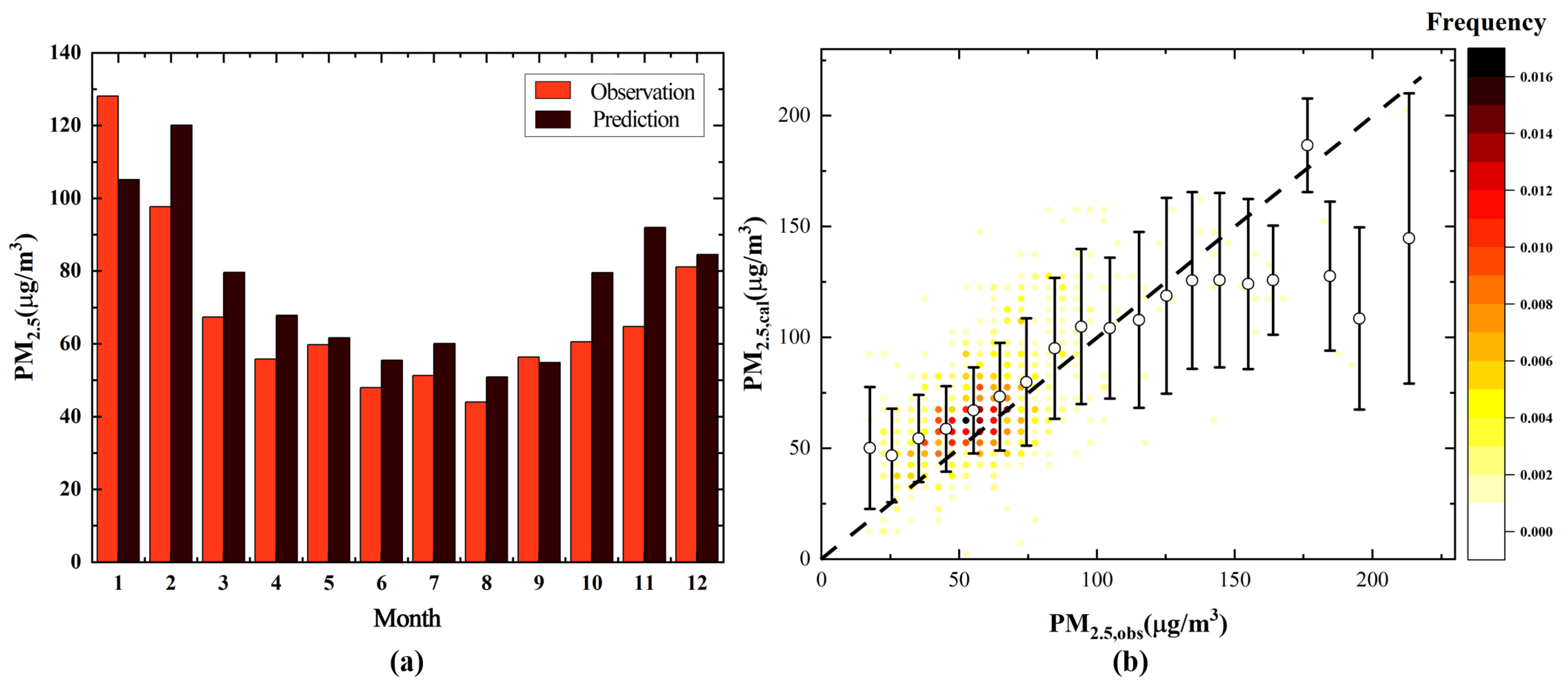
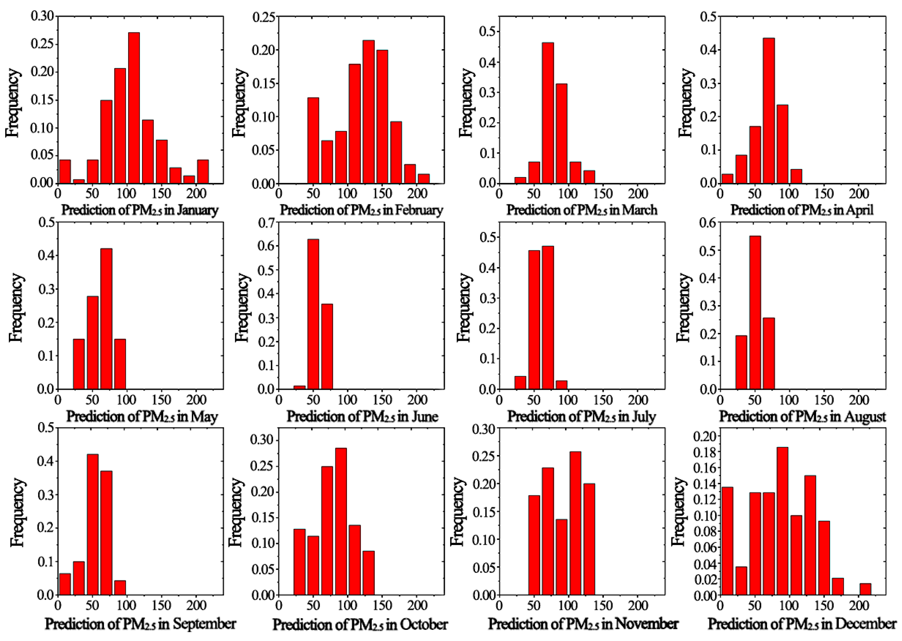
4.3. Intermonth Variation of PM_2.5 Mass Concentration

Based on the BP neural network model constructed above, using the MODIS products and ERA5 meteorological data of Beijing–Tianjin–Hebei–Shanxi in 2017, we obtained the regional monthly PM_2.5 mass concentrations. Figure 4a shows the intermonth changes of satellite-derived PM_2.5 mass concentrations using seasonal models and that compared with ground-based values in Beijing, Tianjin, Hebei, and Shanxi in 2017. The monthly PM_2.5 mass concentration shows obvious inter-monthly changes. The monthly PM_2.5 mass concentrations are less than 60 μg/m³ from June to August; they increased significantly from December to February (more than 80 μg/m³), which is consistent with the observed intermonth variation, with an average relative deviation of 17.7%. Figure 4b shows the validation of the satellite-derived monthly PM_2.5 mass concentration in 2017. The binning error (dots and error bars) is close to the 1:1 line, and there is a characteristic of overestimation at low values and underestimation at high values. The mass concentration of near ground PM_2.5 is concentrated in the range of 20 to 125 μg/m³, which accounts for about 92.2% of the total samples. The mean value of satellite-derived monthly PM_2.5 mass concentration is 78.98 μg/m³, which is 17.04% overestimated compared with the ground-based value (67.48 μg/m³). The result by Yan et al. [29] is 69.38 μg/m³, which is roughly consistent with the results of this study. The underestimation of the satellite-derived monthly PM_2.5 mass concentration occurs when concentration is above 150 μg/m³, which can be explained by the underestimation of AOD in the case of heavy pollution [14,30]. The slight overestimation occurs at the concentration below 75 μg/m³, which may be related to the bias of cloud identification in the satellite inversion algorithm.

Figure 5 shows the frequency density distribution of near-surface PM_2.5 mass concentration, month-by-month, in 2017. The PM_2.5 frequency density basically obeys a unimodal distribution, which is consistent with Lu’s [31] study. The peak of frequency density distribution from June to September is at the bin of 50 μg/m³, while the peak in the winter (December–February) appears in bins greater than 100 μg/m³. Other monthly peaks fall in between. It indicates that PM_2.5 mass concentration in north China in the winter is significantly higher, and the air quality in the summer is obviously better than that in other seasons in 2017.

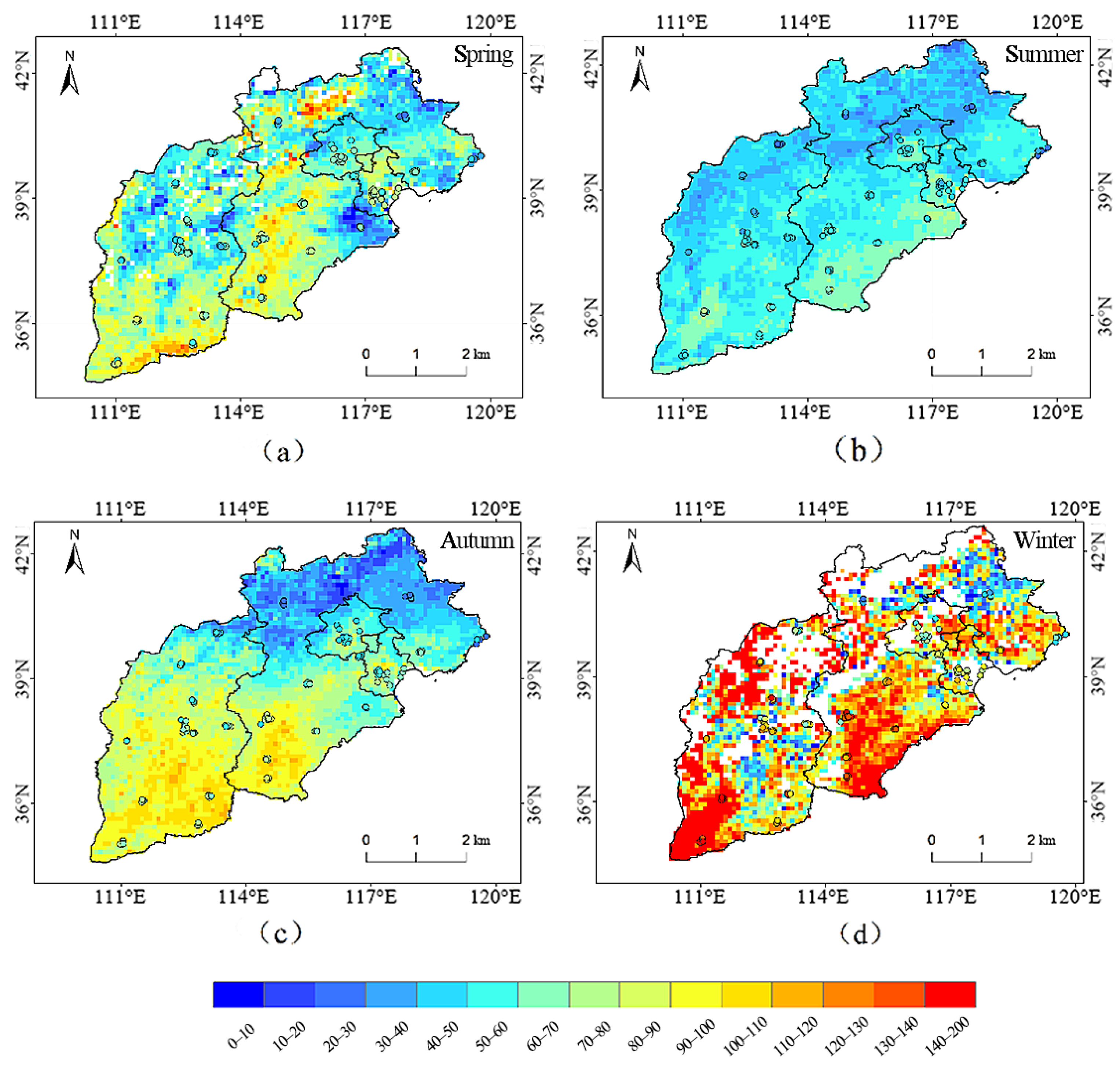
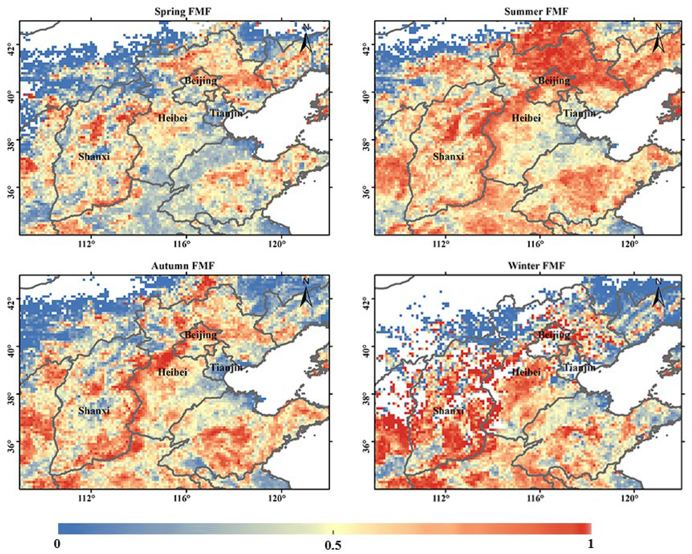
4.4. Spatial Distribution of PM_2.5 Mass Concentration

Figure 6 shows the spatial distribution of the quarterly average of the near-surface PM_2.5 mass concentration in the Beijing–Tianjin–Hebei–Shanxi region in 2017. The blank regions in Figure 6 is due to satellite-retrieved AOD missed in high surface reflectivity. More blank regions show up in the winter because there are more snowy/cloudy/rainy days in winter [3,32]. In terms of spatial distribution, the PM_2.5 mass concentration obtained by this study and ground station observation has a high similarity, with the characteristics of being high in the winter and low in the summer. The PM_2.5 concentration shows similar spatial patterns in different seasons. The area north of 40° N was less polluted. The Taihang Mountains were the clear boundaries of the pollution intensity. The pollution in the southeast of the mountain range was significantly higher than that in the northwest, and there are obvious sudden changes where the terrain changes. Southern Hebei and Southern Shanxi are the most polluted areas, the surrounding areas are second only to this area, and the pollution in the north–south direction is slightly higher than that in the east–west direction. This spatial distribution is consistent with the prediction results in the study of Li et al. [28] using random forests.

The PM_2.5 concentration in Beijing–Tianjin–Hebei–Shanxi is highest in the winter (Figure 6d), lowest in the summer (Figure 6b), and similar in the spring (Figure 6a) and autumn (Figure 6c). In the winter, the average monthly PM_2.5 concentration in Beijing, Tianjin, Hebei, and Shanxi exceeded 120 μg/m³. The pollutants less likely to diffuse were mainly caused by the high atmospheric humidity, the low temperature, and the small surface wind speed. The temperature inversion and heating in the Beijing–Tianjin–Hebei–Shanxi region also can have a significant impact on PM_2.5 pollution. In the spring, sunshine duration increases compared to that in the winter; the vertical exchange is strengthened, so that the PM_2.5 concentration decreases. In the summer, the precipitation and sunshine duration are the largest and the top of the boundary layer is the highest, the pollutant diffusion conditions are the best in the four seasons, and the PM_2.5 concentration in China is the lowest, but the Beijing–Tianjin–Hebei–Shanxi region is still generally greater than 35 μg/m³. In the autumn, the atmospheric stratification is relatively stable, the wind speed is low, so that the PM_2.5 pollution begins to accumulate.

5. Conclusions and Discussion

Based on satellite remote sensing products and meteorological data, we used the BP neural network to establish a prediction model for the PM_2.5 mass concentration. The mean impact value (MIV) was used to analyze the impacts of remote sensing variables on the prediction of the PM_2.5 mass concentration. There were three groups of models trained to detect the seasonal influences, and then the seasonal models were applied to predict the spatial distribution of the PM_2.5 mass concentrations. We found that the BP network model was effective at revealing the spatial and temporal distributions of the regional PM_2.5 mass concentrations. The predicted PM_2.5 mass concentrations in different seasons are affected by changes of surface reflectance and dominant particle size, which provides experimental support for seasonal training and the use of multivariate remote sensing data. The model, considering seasonal factors, is better than the annual model in all aspects. The PM_2.5 mass concentration predicted by the seasonal models shows strongly seasonal changes, while the spatial pattern is similar, which can be related to the distribution of anthropogenic emissions and topographic features in the region. Compared with the ground-based observations, the correlation coefficients (R) in the four seasons are all above 0.7, indicating that the seasonal models can predict PM_2.5 mass concentration well.

This work contributes to the evolution of inputting spectral AOD from multiple algorithms and fine AOD products for PM_2.5 prediction. In addition to some land properties, quality control valuables and accuracy valuables are simultaneously inputted in the model to improve the prediction. However, there are some limitations of this model. The sufficient data volume is a necessary guarantee for establishing an available model based on machine learning methods, although many studies [21,23,32,33,34,35] have built PM_2.5 estimation models using one-year data. Considering that only one-year data were used in the training in this study, the model has limited accuracy and is relatively weak in predicting PM_2.5 mass concentration beyond 2017. Based on the development of satellite technologies and the inversion algorithm, the estimation accuracy of PM_2.5 can be improved in steps in the future.

Although we obtained a good seasonal model to predict PM_2.5 mass concentrations, there is still room for improvement. In this study, the model inputs only considered satellite products and meteorological parameters, whereas other parameters, such as geographic elevation data, can be added to test the impacts on the network performance to optimize the PM_2.5 predicting model. Moreover, because the PM_2.5 concentration of a site has a spatial relationship with surrounding sites, a convolutional neural network can be adopted to take the data of surrounding areas into account on the input. Moreover, PM_2.5 has obvious periodicity in time, and a time series neural network or other recurrent networks can be used for modeling in the future.

References

1. Sicard, P.; Khaniabadi, Y.O.; Perez, S.; Gualtieri, M.; De Marco, A. Effect of O3, PM10 and PM2.5 on Cardiovascular and Respiratory Diseases in Cities of France, Iran and Italy. Environ. Sci. Pollut. Res. 2019, 26, 32645–32665. [Google Scholar] [CrossRef] [PubMed]
2. Huang, C.; Moran, A.E.; Coxson, P.G.; Yang, X.; Liu, F.; Cao, J.; Chen, K.; Wang, M.; He, J.; Goldman, L.; et al. Potential Cardiovascular and Total Mortality Benefits of Air Pollution Control in Urban China. Circulation 2017, 136, 1575–1584. [Google Scholar] [CrossRef] [PubMed]
3. Geng, G.; Zhang, Q.; Martin, R.; van Donkelaar, A.; Huo, H.; Che, H.; Lin, J.; He, K. Estimating Long-Term PM2.5 Concentrations in China Using Satellite-Based Aerosol Optical Depth and a Chemical Transport Model. Remote Sens. Environ. 2015, 166, 262–270. [Google Scholar] [CrossRef]
4. Huang, K.; Xiao, Q.; Meng, X.; Geng, G.; Wang, Y.; Lyapustin, A.; Gu, D.; Liu, Y. Predicting Monthly High-Resolution PM2.5 Concentrations with Random Forest Model in the North China Plain. Environ. Pollut. 2018, 242, 675–683. [Google Scholar] [CrossRef]
5. Li, H.; Zhang, Q.; Zhang, Q.; Chen, C.; Wang, L.; Wei, Z.; Zhou, S.; Parworth, C.; Zheng, B.; Canonaco, F.; et al. Wintertime Aerosol Chemistry and Haze Evolution in an Extremely Polluted City of the North China Plain: Significant Contribution from Coal and Biomass Combustion. Atmos. Chem. Phys. 2017, 17, 4751–4768. [Google Scholar] [CrossRef] [Green Version]
6. Tian, J.; Chen, D. A Semi-Empirical Model for Predicting Hourly Ground-Level Fine Particulate Matter (PM2.5) Concentration in Southern Ontario from Satellite Remote Sensing and Ground-Based Meteorological Measurements. Remote Sens. Environ. 2010, 114, 221–229. [Google Scholar] [CrossRef]
7. Hoff, R.M.; Christopher, S.A. Remote Sensing of Particulate Pollution from Space: Have We Reached the Promised Land? J. Air Waste Manag. Assoc. 2009, 59, 645–675. [Google Scholar] [CrossRef]
8. Xie, Z.Y.; Liu, H.; Tang, X.M. Correlation Analysis between Modis Aerosol Optical Depth and PM10 Concentration over Beijing. Acta Sci. Circumstantiae 2015, 35, 3292–3299. [Google Scholar]
9. Zhang, Y.; Li, Z.; Bai, K.; Wei, Y.; Xie, Y.; Zhang, Y.; Ou, Y.; Cohen, J.; Zhang, Y.; Peng, Z.; et al. Satellite Remote Sensing of Atmospheric Particulate Matter Mass Concentration: Advances, Challenges, and Perspectives. Fundam. Res. 2021, 1, 240–258. [Google Scholar] [CrossRef]
10. Lin, H.-F.; Xin, J.-Y.; Zhang, W.-Y.; Wang, Y.-S.; Liu, Z.-R.; Chen, C.-L. Comparison of Atmospheric Particulate Matter and Aerosol Optical Depth in Beijing City. Huan Jing Ke Xue Huanjing Kexue 2013, 34, 826–834. [Google Scholar]
11. Xin, J.; Zhang, Q.; Wang, L.; Gong, C.; Wang, Y.; Liu, Z.; Gao, W. The Empirical Relationship between the PM2.5 Concentration and Aerosol Optical Depth over the Background of North China from 2009 to 2011. Atmos. Res. 2014, 138, 179–188. [Google Scholar] [CrossRef]
12. Zhang, Y.; Li, Z. Remote Sensing of Atmospheric Fine Particulate Matter (PM2.5) Mass Concentration near the Ground from Satellite Observation. Remote Sens. Environ. 2015, 160, 252–262. [Google Scholar] [CrossRef]
13. Zhang, Y.; Li, Z.; Chang, W.; Zhang, Y.; de Leeuw, G.; Schauer, J.J. Satellite Observations of PM2.5 Changes and Driving Factors Based Forecasting over China 2000–2025. Remote Sens. 2020, 12, 2518. [Google Scholar] [CrossRef]
14. Wei, Y.; Li, Z.; Zhang, Y.; Chen, C.; Xie, Y.; Lv, Y.; Dubovik, O. Derivation of PM10 Mass Concentration from Advanced Satellite Retrieval Products Based on a Semi-Empirical Physical Approach. Remote Sens. Environ. 2021, 256, 112319. [Google Scholar] [CrossRef]
15. Van Donkelaar, A.; Martin, R.V.; Brauer, M.; Kahn, R.; Levy, R.; Verduzco, C.; Villeneuve, P.J. Global Estimates of Ambient Fine Particulate Matter Concentrations from Satellite-Based Aerosol Optical Depth: Development and Application. Environ. Health Perspect. 2010, 118, 847–855. [Google Scholar] [CrossRef] [PubMed] [Green Version]
16. Van Donkelaar, A.; Martin, R.V.; Li, C.; Burnett, R.T. Regional Estimates of Chemical Composition of Fine Particulate Matter Using a Combined Geoscience-Statistical Method with Information from Satellites, Models, and Monitors. Environ. Sci. Technol. 2019, 53, 2595–2611. [Google Scholar] [CrossRef] [Green Version]
17. Van Donkelaar, A.; Martin, R.V.; Park, R.J. Estimating Ground-Level PM2.5 Using Aerosol Optical Depth Determined from Satellite Remote Sensing. J. Geophys. Res. Atmos. 2006, 111, 7436–7444. [Google Scholar] [CrossRef]
18. Van Donkelaar, A.; Martin, R.V.; Pasch, A.N.; Szykman, J.J.; Zhang, L.; Wang, Y.X.; Chen, D. Improving the Accuracy of Daily Satellite-Derived Ground-Level Fine Aerosol Concentration Estimates for North America. Environ. Sci. Technol. 2012, 46, 11971–11978. [Google Scholar] [CrossRef]
19. van Donkelaar, A.; Martin, R.V.; Spurr, R.J.D.; Drury, E.; Remer, L.A.; Levy, R.C.; Wang, J. Optimal Estimation for Global Ground-Level Fine Particulate Matter Concentrations. J. Geophys. Res. Atmos. 2013, 118, 5621–5636. [Google Scholar] [CrossRef] [Green Version]
20. Van Donkelaar, A.; Martin, R.V.; Brauer, M.; Boys, B.L. Use of Satellite Observations for Long-Term Exposure Assessment of Global Concentrations of Fine Particulate Matter. Environ. Health Perspect. 2015, 123, 135–143. [Google Scholar] [CrossRef] [Green Version]
21. Hu, X.; Waller, L.A.; Al-Hamdan, M.Z.; Crosson, W.L.; Estes, M.G., Jr.; Estes, S.M.; Quattrochi, D.A.; Sarnat, J.A.; Liu, Y. Estimating Ground-Level PM2.5 Concentrations in the Southeastern Us Using Geographically Weighted Regression. Environ. Res. 2013, 121, 1–10. [Google Scholar] [CrossRef] [PubMed]
22. Li, T.; Shen, H.; Yuan, Q.; Zhang, L. A Locally Weighted Neural Network Constrained by Global Training for Remote Sensing Estimation of PM2.5. IEEE Trans. Geosci. Remote Sens. 2021, 60, 1–13. [Google Scholar] [CrossRef]
23. Li, L.; Chen, B.; Zhang, Y.; Zhao, Y.; Xian, Y.; Xu, G.; Zhang, H.; Guo, L. Retrieval of Daily PM2.5 Concentrations Using Nonlinear Methods: A Case Study of the Beijing–Tianjin–Hebei Region, China. Remote Sens. 2018, 10, 2006. [Google Scholar] [CrossRef] [Green Version]
24. Xu, X.; Tian, Y.; Xiao, Y.; Jiang, W.; Tian, L.; Liu, J. Study on the Spatial Distribution Characteristics and the Drivers of Aqi in North China. Acta Sci. Circumstantiae 2017, 8, 3085–3096. [Google Scholar]
25. Deng, W.-Y.; Zheng, Q.-H.; Chen, L.; Xu, X.-B. Research on Extreme Learning of Neural Networks. Chin. J. Comput. 2010, 33, 279–287. [Google Scholar] [CrossRef]
26. Sun, B.L.; Sun, H.; Zhang, C.N.; Shi, J.W.; Zhong, D.Q. Forecast of Air Pollutant Concentrations by Bp Neural Network. Acta Sci. Circumstantiae 2017, 37, 1864–1871. [Google Scholar]
27. Guo, L.; Fan, B.; Zhang, F.; Jin, Z.; Lin, H. The Clustering of Severe Dust Storm Occurrence in China from 1958 to 2007. J. Geophys. Res. Atmos. 2018, 123, 8035–8046. [Google Scholar] [CrossRef]
28. Li, Y.; Xue, Y.; Guang, J.; She, L.; Fan, C.; Chen, G. Ground-Level PM2.5 Concentration Estimation from Satellite Data in the Beijing Area Using a Specific Particle Swarm Extinction Mass Conversion Algorithm. Remote Sens. 2018, 10, 1906. [Google Scholar] [CrossRef] [Green Version]
29. Yan, D.; Lei, Y.; Shi, Y.; Zhu, Q.; Li, L.; Zhang, Z. Evolution of the Spatiotemporal Pattern of Pm2. 5 Concentrations in China–a Case Study from the Beijing-Tianjin-Hebei Region. Atmos. Environ. 2018, 183, 225–233. [Google Scholar] [CrossRef] [Green Version]
30. Wei, Y.; Li, Z.; Zhang, Y.; Chen, C.; Dubovik, O.; Xu, H.; Li, K.; Chen, J.; Wang, H.; Ge, B.; et al. Validation of Polder Grasp Aerosol Optical Retrieval over China Using Sonet Observations. J. Quant. Spectrosc. Radiat. Transf. 2020, 246, 106931. [Google Scholar] [CrossRef]
31. Lu, J.; Zhang, Y.; Chen, M.; Wang, L.; Zhao, S.; Pu, X.; Chen, X. Estimation of Monthly 1 Km Resolution PM2.5 Concentrations Using a Random Forest Model over “2 + 26” Cities, China. Urban Clim. 2021, 35, 100734. [Google Scholar] [CrossRef]
32. Zhan, Y.; Luo, Y.; Deng, X.; Chen, H.; Grieneisen, M.L.; Shen, X.; Zhu, L.; Zhang, M. Spatiotemporal Prediction of Continuous Daily PM2.5 Concentrations across China Using a Spatially Explicit Machine Learning Algorithm. Atmos. Environ. 2017, 155, 129–139. [Google Scholar] [CrossRef]
33. Chen, J.; Yin, J.; Zang, L.; Zhang, T.; Zhao, M. Stacking Machine Learning Model for Estimating Hourly PM2.5 in China Based on Himawari 8 Aerosol Optical Depth Data. Sci. Total Environ. 2019, 697, 134021. [Google Scholar] [CrossRef] [PubMed]
34. Li, T.; Shen, H.; Yuan, Q.; Zhang, X.; Zhang, L. Estimating Ground-Level PM2.5 by Fusing Satellite and Station Observations: A Geo-Intelligent Deep Learning Approach. Geophys. Res. Lett. 2017, 44, 11–985. [Google Scholar] [CrossRef] [Green Version]
35. Liu, J.; Weng, F.; Li, Z. Satellite-Based PM2.5 Estimation Directly from Reflectance at the Top of the Atmosphere Using a Machine Learning Algorithm. Atmos. Environ. 2019, 208, 113–122. [Google Scholar] [CrossRef]
Figure 1. The study area including Beijing, Tianjin, Hebei, and Shanxi, and the PM2.5 monitoring sites. The circle and triangle symbols are the PM2.5 monitoring sites, but the triangle symbols have lower accuracy of the model prediction.
Atmosphere 13 00825 g001
Figure 2. Modeling flow.
Atmosphere 13 00825 g002
Figure 3. Fitting performance of training set in each season.
Atmosphere 13 00825 g003
Figure 4. (a) The inter-monthly changes of satellite-derived PM2.5 mass concentration with ground-based values in Beijing, Tianjin, Hebei, and Shanxi in 2017. (b) Validation of satellite-derived monthly PM2.5 mass concentration in 2017. The total number of samples is 1680, and the color scale indicates the frequency of the samples at each gear (5 μg/m3). The black dashed line represents the 1:1 line. Circles and error bars represent the statistical mean and standard deviation of the samples over each statistical interval (10 μg/m3).
Atmosphere 13 00825 g004
Figure 5. Frequency density map of monthly mean station PM2.5 mass concentration estimated by remote sensing in 2017.
Atmosphere 13 00825 g005
Figure 6. Comparison of the seasonally averaged PM2.5 mass concentration values of Beijing–Tianjin–Hebei–Shanxi in 2017 and ground observation points. (a) Spring, (b) Summer, (c) Autumn, (d) Winter.
Atmosphere 13 00825 g006