Article

Assessment of Integrated Aerosol Sampling Techniques in Indoor, Confined and Outdoor Environments Characterized by Specific Emission Sources

1
INSTM and Department of Mechanical and Industrial Engineering, University of Brescia, via Branze, 38, 25123 Brescia, Italy
2
Department of Mathematics and Physics, Università Cattolica del Sacro Cuore, via Musei 41, 25121 Brescia, Italy
3
Sensor Laboratory, Department of Information Engineering (DII), University of Brescia, via Branze, 38, 25123 Brescia, Italy
4
Department of Medical and Surgical Specialties, Radiological Sciences, and Public Health, University of Brescia, Viale Europa, 11, 25123 Brescia, Italy
5
Department of Environmental Health, Robert Stempel College of Public Health and Social Work, Florida International University, 11200 SW 8th Street AHC5, Miami, FL 33199, USA
*
Authors to whom correspondence should be addressed.
Submission received: 24 March 2021 / Revised: 3 May 2021 / Accepted: 7 May 2021 / Published: 11 May 2021

Abstract

:
This paper highlights advantages and drawbacks due to the use of portable and low-cost devices for aerosol sampling, showing their performances during an aerosol monitoring campaign with the parallel use of the gravimetric sampling reference method and a cascade impactor. A specific monitoring campaign was held running all instruments in parallel in indoor, confined, and outdoor environments characterized by local emission sources or particulate matter background concentrations. PM2.5 concentrations were used to compare data emerging from the different instruments adopted. Significant underestimation of PM2.5 emerged when comparing data coming from optical sensors with those estimated by the cascade impactor, whose data resulted in being coherent with gravimetric determination, integrated over the same sampling time. A cause–effect relationship between PM2.5 concentrations and specific emission sources was found when observing the daily patterns of all the real-time sampling devices. It emerged that optical devices are useful for detecting concentration trends, the presence of peak values, or changes in the background value, even if with limited accuracy and precision. The comparison with particle size distributions obtained by the cascade impactor data allowed us to define which particle sizes are not detected by different optical devices, evidencing a low representativeness of optical low-cost sensors for health exposure measurements. The correlations among the specific particle size fractions detected by the cascade impactor and their specific emission sources were particularly high for car emissions in a semi-confined garage area.

1. Introduction

Aerosol monitoring is extremely important since the respirable suspended particles (hereafter denoted as RSP, commonly referred to as PM10) are presently considered one of the most critical atmospheric pollutants, mainly in urban areas. Actually, PM10 concentrations often exceed the daily limit value according to the Directive 2008/50/EC [1], especially in winter when adverse meteorological conditions (i.e., thermal inversions) confine pollutants near ground level [2]. Furthermore, the health impact of aerosol is scientifically recognized [3,4,5]. PM10, for example, can penetrate the upper respiratory tract, and PM2.5 can reach the secondary lungs and bronchi [6]. In particular, the effects of exposure to PM2.5 on stroke, dementia, Alzheimer’s disease, autism spectrum disorder (ASD), Parkinson’s disease, and mild cognitive impairment (MCI) had been scientifically demonstrated [7]. For almost 20 years aerosol monitoring has started to focus not only on particle mass (PM) but also on particle number (PN) in order to better assess the health impact due mainly to ultrafine (1–100 nm) and fine (100–1000 nm) particles [8,9]. Actually, in urban areas the size distributions of particles present PN peaks (between 2000 and 4000 cm−3) in the ultrafine region [10,11,12] even if their contribution as particle mass (PM) is negligible. The parallel sampling of PN and PM is thus becoming more and more important in the aerosol monitoring field. Even indoor aerosol monitoring is capturing the attention of researchers in the field, since people spend more than 80% of their time in closed environments [13,14], and instantaneous PN values could increase by more orders of magnitude with respect to background levels after the activation of aerosol indoor sources [11,15].
The harmfulness of atmospheric particulate on human health depends not only on particles size but also on chemical composition. Indeed, during recent years, substantial improvements were achieved in the chemical characterization and identification of the main atmospheric aerosol components [16]. Inorganic species represent more than 1% of total RSP mass and their sources are identified as crustal elements (silicon, aluminum, iron, calcium, carbonate), sea-salt aerosol (sodium chloride), inorganic secondary species (ammonium nitrate and sulphate), and primary anthropogenic species (elemental carbon). Organic compounds instead represent from 20 up to 60% of RSP mass and include a wide variety of individual species such as harmful compounds or tracers of specific emission sources [17] and biologic material [18]. These measurements are performed on PM10 or PM2.5 filters coming from the reference system (gravimetric samplers) so that the chemical speciation is averaged over all particles collected on them. Nevertheless, particles contained in the atmospheric aerosol cover five orders of magnitude, from a few nm up to 100 µm [16], so complete monitoring coverage of them needs more devices characterized by different physical principles. A wide variety of instruments for aerosol monitoring is present on the market and their technical features could be very different. For example, there are real-time instruments based on laser scattering (optical particle counters, OPC) able to detect particles with optical diameters above 300 nm [19]; gravimetric devices able to detect PM1, PM2.5, and PM10 depending on their inlet impactors; real-time cascade impactors able to detect different particle fractions on different stages from 10 nm up to 10 µm; and condensing particle counters (CPC) able to detect nanometric particles through their enlargement due to butanol or water condensation followed by optical detection. Real-time instruments such as cascade impactors, and OPC and CPC instruments for aerosol monitoring could be characterized by high precision and sensitivity but they can reach costs up to tens of thousands of euros and require significant resources for their constant maintenance and calibration [20,21], so a capillary monitoring of aerosol concentrations could only be performed by less precise and sensitive but low-cost (from EUR 10 up to EUR 1000 indicatively), small, easy-to-manage, and portable (their dimension is up to one tenth of the size of the instruments used in air-quality monitoring networks) sensors [19]. Low-cost sensors are based on the optical detection of particles through laser scattering, counting particles with an optical diameter under 1, 2.5, or 10 µm and indirectly evaluating PM1, PM2.5, and PM10, assuming for all particles a unit density and a spherical shape [22,23]. The indirect calculation of particle mass from the particle concentration number is often discouraged if not accompanied by reference measurements [19,24,25]. The real density and shape of particles as well as their color and refractive index can affect the evaluation of their size distribution [26,27,28]. Nevertheless, the availability of diffuse differential concentrations in terms of PM2.5 or PM10 over a territorial domain could help a local or regional administrator in understanding eventual critical sites to implement the right policies to abate RSP [21].
Along with the estimation of RSP concentrations, other integrated low-cost sensors in the same monitoring device can evaluate parameters such as temperature, humidity, and carbon dioxide concentrations to additionally estimate the air quality index (EEA, n.d.). Some examples taken from the literature [19,23] are given by the following devices: OPC-N1 (Alphasense, Essex, UK), the DC1100 Pro (Dylos, Riverside, CA, USA, GP2Y1010 (Sharp, Sakay City, Japan), Kobe, Japan, and AirVisual Pro (IQAir AG, Goldach, Switzerland). New solutions in the field of low-cost RSP sensors are continuously under study, including devices able to detect nanoparticles using different technical principles [29].
Low-cost sensors can be deployed in great quantities and connected in devoted air-quality networks. The resulting measurements are sent to dedicated platforms (e.g., AirCasting, AirVisual) for global collection and data sharing [23]. These widespread devices may provide high temporal and spatial resolution if we really understand and critically evaluate the capabilities and characteristics of the data they provide, allowing the development of PM1, PM2.5, and PM10 concentration maps at a global level to drive local policies for PM abatement. To assure their effective usefulness as aerosol monitoring devices, they must be tested in parallel to reference instruments. Measurements should be performed indoors and outdoors to characterize different aerosol sources and meteorological conditions that can greatly impact low-cost sensor performance [25,30]. Optical devices can be affected by high relative humidity conditions that could lead to an underestimation of PM. Furthermore, the instability of the flow of a low-cost sensor can alter the quantity of particles being sampled. An intercomparison of parallel aerosol measurements allows a critical evaluation of the potentialities of a large-scale implementation of low-cost sensors since data of poor or unknown quality are less useful than no data at all [31]. To the best of our knowledge, the literature reports mainly intercomparison studies of outdoor aerosol monitoring among optical devices (standard analyzers and/or low-cost sensors) and gravimetric samplers used as reference. A more comprehensive study including devices with different working principles and analysis methods for PM determination is needed.
In this paper, measurements taken with optical low-cost sensors, gravimetric samplers, and a cascade impactor are directly compared for quantitative determination of PM2.5 concentration and to estimate detection limits. Our research aims to assess the performance of low-cost sensors in comparison with other technical devices to better understand potentialities and drawbacks, and their usefulness for health impact assessment.

2. Materials and Methods

The present research foresaw the integration of more atmospheric aerosol monitoring devices to detect particle number and mass due to the activation of specific particle sources.
The tests were conducted in the northeast of Italy (the city of Brescia), inside the Po Valley, characterized by high pollution levels [32]. The places selected for sampling differed based on environmental conditions and/or location. Three locations were considered: an indoor warehouse (laboratory of civil and construction engineering), a garage, and an outdoor area adjacent to the warehouse (Figure 1).
With reference to the environmental conditions in the warehouse, the monitoring period comprised both the presence of building and construction activities (referred to as “indoor busy”) and the absence of building work (referred to as “indoor quiet”). The outdoor area was characterized by the occasional presence of smokers in the surroundings. Finally, the garage events were only related to cars passing by. The sampling period covered 12 workdays in March 2018. The calendar of measurements is reported in the Supplementary Materials (Figure S1). Labels assigned to each day identify the specific monitoring site and environmental conditions.
Aerosol concentrations were monitored by running different instruments in parallel. In particular, the integrated monitoring system comprised two low-cost instruments characterized by the optical detection of particles, a gravimetric sampler, and a cascade impactor. In the following paragraphs we provide details about the technical features of all instruments.
The Electrical Low-Pressure Impactor (ELPI+, Dekati, Tampere, Finland) provides the real-time particle number size distribution in a wide dimensional range (6 nm to 10 µm) with a sampling frequency up to 10 Hz. For the measurements foreseen by this research the sampling frequency was set to 1 Hz. It also indirectly estimates PM10–PM2.5–PM1 with the usual approximations of particle unit density and sphericity. The measurement principle is based on the unipolar charging of particles through a discharge achieved by a positive high voltage of approximately 3.5 kV. To achieve stable charging conditions, the discharge current is kept at a constant value of 1 µA. The following size classification according to the particles’ aerodynamic diameter is given by the impact of particles on 14 different impactor stages [29] characterized by different cut-off efficiencies reported in Table 1.
Particles with aerodynamic diameters lower than the D50% value are ideally collected in the following stages in the air flow direction: from stage 14 to filter stage F, whereas particles with aerodynamic diameters between the D50% values of two consecutive stages are collected in the stage with the lower D50%. The 14 impactor stages of the instrument are electrically insulated and connected to sensitive electrometers. Currents measured by each electrometer are directly proportional to the particle number concentrations with calibration factors provided by the manufacturer [33]. The downstream pressure is measured and can be set to the manufacturer-specified value of 40 mbar by adjusting a control valve, located between the filter stage and the connection to the external vacuum pump, with a flow rate of 10 L/min. The ELPI+ can be used for gravimetric measurements by calculating the weight difference of the filters placed on each impactor stage. However, for this work greased Al foils were used to avoid particles bouncing and to improve the accuracy of particle determination. Thus, no gravimetric data were extracted.
The customized kit for outdoor air quality measurements (hereafter called KORA, Acronet, Savona, Italy) is a remote meteorological station that measures PM2.5 by extractive sensing using a high-flow pump operating at 10 L/min along with air temperature, relative humidity, and atmospheric pressure. Data are registered with a time resolution of 5 s and sent to the remote platform, where they are privately stored and can be downloaded.
The personal modular impactor (PMI, SKC, Blandford Forum Dorset, UK) is a portable gravimetric sampler characterized by a single inertial impactor that collects PM2.5 by an extractive method using a Leland Legacy SKC pump operating at 10 L/min and collecting particles onto a Teflon filter membrane with a pore size of 2 µm, weighed before and after the sampling to evaluate particulate mass. Sampling was performed on the same filter over all weekdays during the first two weeks and on one filter per day during the last two days, to collect one filter per environment. Filters were weighed with a microbalance (model XS3DU, Mettler Toledo, Milano, Italy) characterized by a sensibility of 0.5 µg (1 μg readability between 0–0.8 g and 10 μg readability up to 3.1 g).
The AirVisual Pro is a real time aerosol sampler with time resolution: 10 s based on laser light scattering by particles for the indirect monitoring of PM2.5 concentrations, integrated with low-cost sensors to monitor CO2 concentrations and meteorological parameters (air temperature and relative humidity). Within the measuring chamber, a laser beam hits the particles and light is scattered in different directions. A photodetector can count particles according to the light scattering angle through the measurements of single pulses. The device can detect particles with optical diameters ranging from about 0.3 µm to 2.5 µm. The device also provides the concentration of PM10 calculated by an algorithm using the concentration of PM2.5 [34,35].
Statistical analysis of the data was performed with the JMP Software (SAS Institute srl, Milano, Italy). Multivariate statistical analysis was performed with the PARAFAC method. Experimental data were arranged in a three-dimensional array, collecting the instruments in the first mode, the PM concentrations in the second mode, and the days in the third mode. The final array was represented by a 9 × 401 × 10 matrix. The most useful chemometric method to analyze this kind of data is parallel factor analysis (PARAFAC), which is a generalization of PCA to a higher-order array [36]. The calculation was performed using MATLAB 2019a (MATLAB R2019a, The MathWorks, Inc.: Natick, MA, USA) with an N-Way Toolbox [37] and PLS_Toolbox version 8.9 (Eigenvector Research Inc., Manson, WA, USA).
Images of particulate matter were collected by field emission scanning electron microscope (FE-SEM, model Leo 1525, Zeiss, Germany), operated in the 1–10 KV range.

3. Results and Discussion

3.1. Comparison of Sampling Locations

Sampling locations and environments were selected to be representative of classes where series of known events are present, in addition to the availability of tools to perform the sampling (i.e., electrical connection and protection from the atmospheric events) for eight (8) consecutive hours, approximately from 9 a.m. to 5 p.m. Normally in the warehouse, emission sources are absent and air recirculation is low: This condition is indicated as “indoor quiet.” Occasionally, building work in the presence of extraordinary emission sources is performed: This condition is indicated as “indoor busy.” Direct car exhaust emissions and resuspension of fine particles are present in the garage. Uncontrollable diffuse emissions are present outdoors. All the daily patterns collected with KORA and AirVisual Pro along with the specific events that occurred during the monitoring period are reported in the Supplementary Materials (Figures S2 and S3 and Table S1). Both patterns allowed a simple and immediate evaluation of PM2.5 concentration trends, showing peaks corresponding to the presence of identified emission sources. For a detailed comparison, a one-day representative of each sampling location and environmental conditions was selected. The corresponding PM2.5 daily patterns collected with KORA are reported in Figure 2, with the identification of the most relevant emission sources (see Supplementary Materials Table S1 for the code descriptions).
The locations have different ranges of average concentration values. The average PM2.5 baseline concentrations indoors fell in the range of 4–15 µg/m3 and were clearly influenced by the presence of peaks, up to 40–45 µg/m3 under busy conditions due to emissions from internal combustion engines in the warehouse. During the indoor busy condition, the occurrence of events such as a truck entering the warehouse at 9 a.m. and the following wall demolition at 11 a.m. were reflected over different duration periods, lasting the time needed for full air recirculation in the area investigated. The presence of a forced aspiration near the emission source rapidly abated PM2.5 concentrations. The average PM2.5 concentration outdoors was significantly higher (about 40–50 µg/m3) and quite constant during the day apart from sporadic events due to smokers in the proximity of the sampling device (three sharp peaks were registered between 11:16 and 12:28 a.m.). They were not persistent and did not influence the background value, as it was to be expected in a not-confined area. The PM2.5 concentration range was significantly higher with respect to the previous one, mostly due to the urban contribution, which was higher during these days, as confirmed by the official data of the Regional Agency for Environmental Protection [38] A different situation was recorded in the garage, assumed to be a semi-confined outdoor area and presenting concentrations of up to 60 µg/m3 with peaks corresponding to emissions from car exhausts, mostly concentrated in the early morning. These emissions increased background concentrations over a large duration of time, depending on the natural ventilation conditions.

3.2. Comparison with Reference Gravimetric Measurements

Sampling devices are compared based on two quantitative parameters: the total mass collected during a defined monitoring period and the average daily and/or hourly concentrations. Extractive sampling devices allow both mass and concentration to be calculated if the flow rate is known. Only average concentration values can be used for an external sensing device with no defined flow rate. Given the significance of gravimetric measurement as a reference, the total mass calculated for ELPI+ was compared with the mass collected on the SKC filters and the results are presented in Table 2.
The total mass on the filters was measured gravimetrically by weight difference with the blank filter. The relative percent error (RE%) was determined experimentally by performing three different measurements of the weight of each filter. One filter per environment was prepared (warehouse, outdoors, and garage). Unfortunately, some issues occurred with the SKC pump during the two-week sampling in the warehouse, so the filter was not used for the gravimetric analysis. Therefore, only samples collected in the last two days were considered. The total mass collected by a real-time sampling device can be calculated using Equation (1), where C is the average mass concentration of PM2.5 for each interval ∆t, Q is the pump flow rate (10 L/min for the ELPI+), and Δt is the sampling time interval. The ELPI+ manufacturer provides an RE% value of 1% for PM2.5 concentrations, which was considered as the estimated uncertainty, taking the other factors exactly.
C t   mg / m 3   × Q   m 3 / s × Δ t s = M   mg
The comparison between PMI and ELPI+ data highlighted a very good agreement, with the two values not significantly different. Although the comparison among average concentration values was rough, the one based on the total mass was more precise and allowed us to drive some hypotheses related to the particle size. Indeed, the cascade impactor values of PM2.5 used for the previous calculations were obtained, summing up the data collected in the first 11 stages of the device and able to trap particles with aerodynamic diameters from a few nm up to 2.5 µm. Since it is known that the smallest particles contribute less to the total mass, it is worth noting that this may be partly compensated by their very high number. In addition, it shall be considered that the conversion from number to mass concentration, used to extract ELPI+ data, assumes the unit density of all particles. On this basis, the agreement between PMI and ELPI+ data is even more satisfactory, and it also demonstrates the comparability between these two devices both based on the impaction of particles on filter stages according to their aerodynamic diameter, including the ultrafine range. This was confirmed by SEM images reported in Figure 3, where micrometric-size spongy aggregates of nanoparticles attached to the smooth Teflon filter surface are clearly visible.

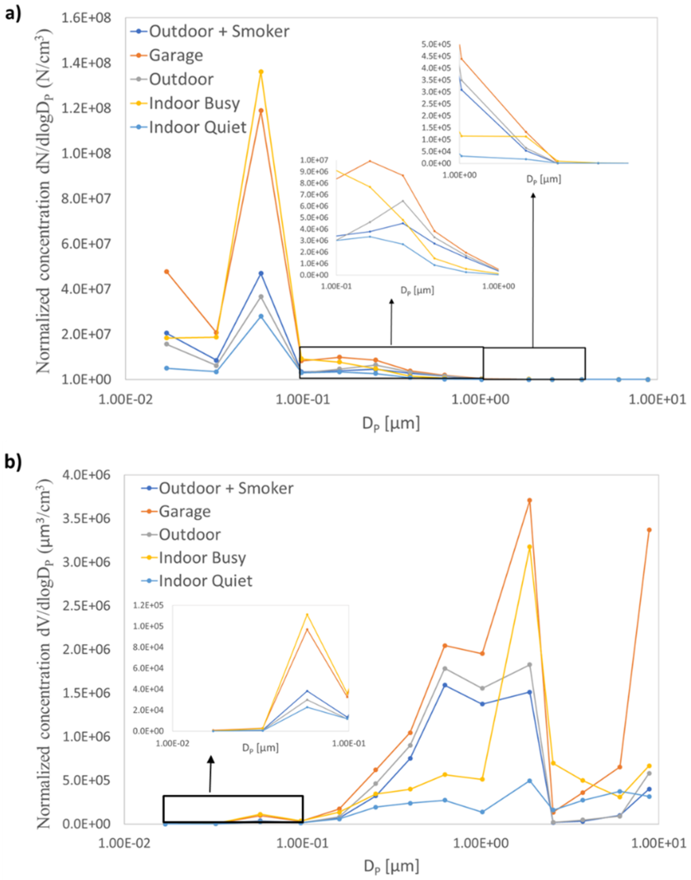
3.3. Granulometric Distribution of the Emitted PM

The comparison of daily PM2.5 patterns of ELPI+ stages showed wide differences. In the same day, the pattern of particles accumulated in near stages were very similar (see Supplementary Materials Figure S4), suggesting their relation, depending obviously on the emission source. To ascertain the possible correlation of fractions, linear correlation plots were used. An example of statistical analysis by linear correlation of data corresponding to Stage 4, highlighting the event of a truck entering the warehouse on the indoor busy day, is reported in the Supplementary Materials (see Figure S5). The linear correlation of data corresponding to the event was clear among the first lower size fractions, which were more representative of the specific emission source, and was progressively lost as the fraction size increased. Linear correlation matrices were built with all the daily patterns (see Table S3), and the PM correlation plots for the most representative environmental condition (garage) are reported in Figure 4.
A unit slope correlation is mostly present, whereas different slopes characterize car exhaust emissions. Indeed, it is known that vehicle emissions depend on the categories, age, and fuel type, but most of them belong to the inhalable fractions of PM2.5–PM10 [39]. When only ultrafine emissions were present the correlation was progressively lost from the lowest to the highest size fractions. Similar considerations could be done for the indoor busy environment (see Table S3 22 March 2018). The correlation here was always present among different fraction size ranges. In particular, the coarse fractions were well correlated, which corresponded to the typical emissions of a construction site where regulations indicate to test coarse PM [40]. This information is fundamental for source apportionment studies.
To determine people exposure to PM for health impact assessments it is important to know the size distribution of particles collected over time. ELPI+ daily patterns in the different stages may be used for that evaluation in the monitoring area. However, daily patterns are not very representative of the contribution of the different emission sources, being mediated over the whole day. For this reason, the portion of patterns corresponding to the exact time of the day when recorded emissions occurred were selected and concentrations over the corresponding hour were summed up. These data were used to build size distribution curves related to five identified emission sources: outdoors with and without the presence of smokers, indoor quiet, during construction work (busy), and garage in the early morning when cars passed by. Normalized particle and volume size distributions are reported in Figure 5, clearly showing a polydisperse curve.
The comparison of normalized data shows that the potential exposure was higher in the outdoor environment, mostly due to the background values and even increased by the presence of smokers, and particularly high in the confined area of the garage where car exhaust emissions occur [41,42,43]. A meaningful increase of inhalable particles was evident in the indoor quiet environment and the contribution of coarse particles was higher when construction work was ongoing.

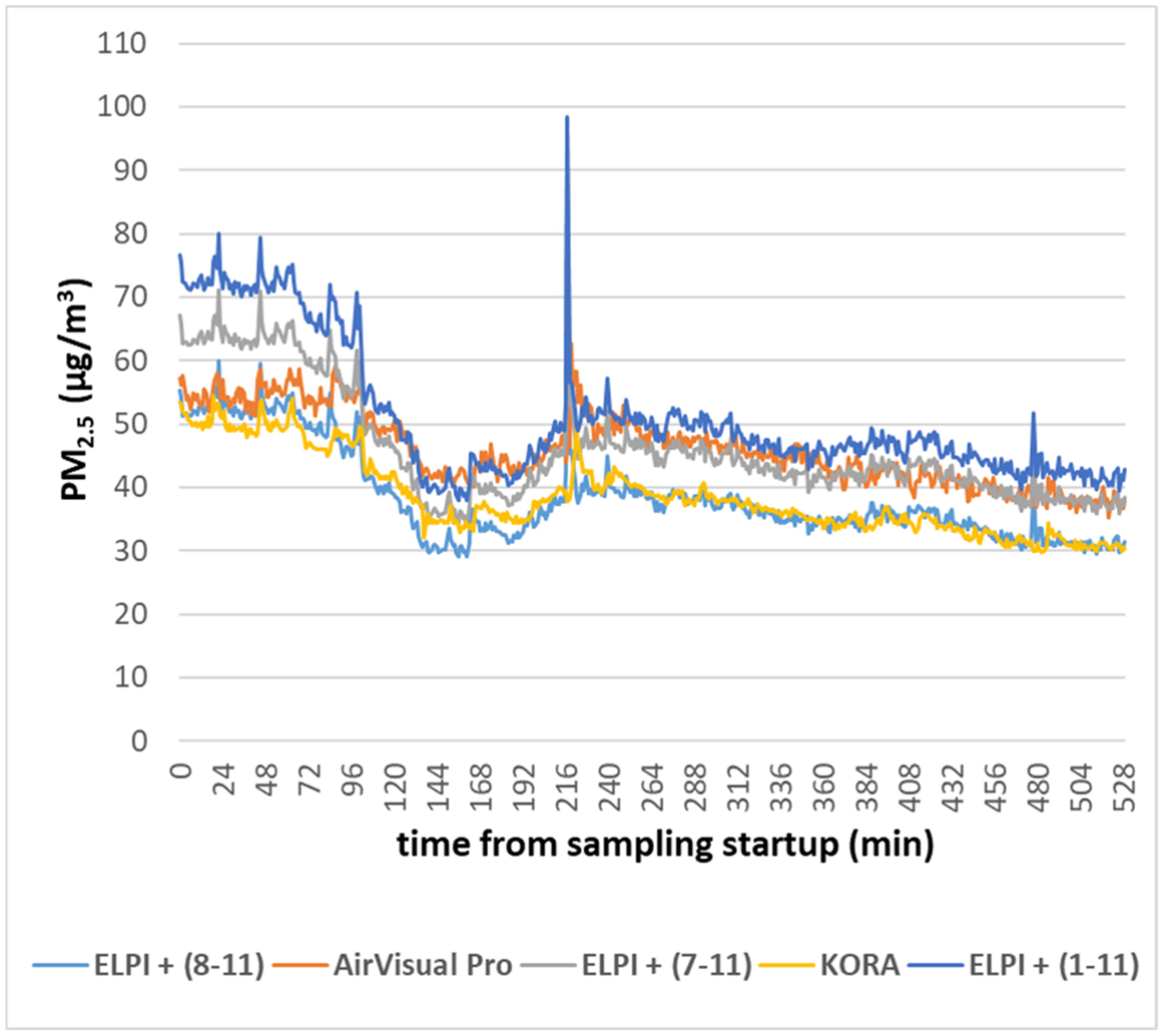
3.4. Comparison of Real-Time Sampling Devices

Given the different sampling frequency of the three devices (ELPI+ 1 Hz, KORA 0.2 Hz, and AirVisual Pro 0.1 Hz), it was necessary to compare average values over the same time interval. Daily average PM2.5 concentrations, including descriptive statistics and uncertainty estimation, are reported in Table 3. The uncertainty estimation in this case was complicated because it was not possible to adopt the error propagation law and there was no data available from the manufacturer. We thus decided to assume the standard deviation based on instrumental sensitivities, equal to 0.5 µg/m3 and 0.05 µg/m3 for AirVisual Pro and KORA, respectively, and calculate the corresponding relative percent error (RE%) of the average values. The comparison among real-time sampling devices confirmed the underestimation of PM2.5 concentrations of both optical systems with respect to the cascade impactor. Given the alignment observed between ELPI+ and SKC data, the above-mentioned underestimation was expected [24,44]. The data reported in Table 3 show the same trend among average concentrations. KORA PM2.5 concentrations lay in the range 65–88%, and those of AirVisual Pro in the range 73–98% with respect to data monitored by the ELPI+.
The comparison based on daily mean concentrations was not representative of the observed PM2.5 concentration trend. Thus, a more in-depth discussion was based on hourly average concentrations. Figure 6 shows the scatter plot and regression lines of the KORA and AirVisual Pro datasets for the whole sampling campaign compared to ELPI+. Data correlation is evident, with linear regression slopes deviating from the unit and decreasing from AirVisual Pro to KORA. The differences among the datasets increases with PM2.5 concentrations. Since the ELPI+ was our reference real-time monitoring device, the AirVisual Pro, despite its small dimensions and easy use, seemed to be more accurate, even less precise, than KORA, but no information about reliability is known. The related Bland–Altman plots [45] are also reported in Figure S6, where the difference between PM2.5 concentration values estimated by specific couples of instruments (ELPI+ and KORA (a), ELPI+ and AirVisual Pro (b), and AirVisual Pro and KORA (c)) are plotted with respect to the average hourly concentrations of measurements collected by the two technical devices. For average PM2.5 concentrations lower than 45 µg/m3, the difference between ELPI+ and KORA/AirVisual Pro concentrations suggested a good agreement between the two monitoring systems and a good representativeness of optical sensors to indirectly evaluate PM2.5 concentrations well beyond the yearly limit value for the protection of human health of 20 µg/m3 [1]. The Bland–Altman plot that compared KORA and AirVisual Pro data showed a good alignment for all the concentrations range, evidencing that they are based on the same physical principle (optical particle detection).

3.5. Estimation of the Detection Limits of the Adopted Optical Devices

A deeper understanding of the results obtained with the three real-time sampling devices needs to consider the differences based on the detection methods. The measurement range may be different mainly in terms of detection limits (LOD), which is the minimum dimension of the determinable particles.
The daily PM2.5 concentration patterns of KORA and AirVisual Pro were compared with concentration patterns obtained by summing the PM concentration values associated with all the cascade impactor particle fractions covering the stages from 1 to 11. The efficiency curve of an ideal impactor stage is a step function that only allow particles larger than the cut-off diameter (D50%) to be collected by inertial impaction, whereas all particles smaller than D50% follow the flow and impact in lower stages. In practice, an un-ideal flow through the impactor nozzles determines a true collection efficiency to be S-shaped [46]. Additionally, due to particles bouncing and blowing off, some large particles will go to the lower stages than they should, and due to diffusion, ultrafine particles will stay in the upper stages. For this reason, the erroneous current signal derived by these factors can be significant, so we decided to consider only stages 1–11 for PM2.5 determination by the cascade impactor when comparing data with the ones produced by AirVisual Pro and KORA.
To understand which fractions were excluded from KORA and AirVisual Pro measurements and how this cut may have affected the sampling results, we first selected the garage location due to the uniformity of emission sources. The whole day concentration patterns are compared in Figure 7, based on average concentration per minute to have greater representativeness. Underestimation of KORA along the whole curve is clear, with an asymmetrical shift higher in the first part of the day.
Similar behavior was observed for the AirVisual Pro, whose pattern was nearer to ELPI+ and moved away markedly in that part of the day. The emissions present in the sampled area during the morning included car exhaust, which is known to produce very fine particles [16]. On this basis, we guessed that both the optical devices were not able to detect the lower range of fine particles and thus the smallest fraction of the cascade impactor should not be included in the PM concentration sum for the comparison. Indeed, the dimensional range represented by the 11 stages was very wide, with lower granulometries up to 6 nm (collected on the filter stage F), well below the optically visible range.
The hypothesis was that optical devices cut the particles with average diameters below 250–300 nm, so the ELPI+ stages from 8 to 11 (for simplicity called 8–11) were considered first. A preliminary graphical comparison showed a very good superposition of the KORA and 8–11 patterns throughout the whole day, whereas the agreement with AirVisual Pro was present only in the first two hours of sampling, and the 8–11 pattern was lower in the rest of the day (see Figure 7). For this reason, a new pattern also including fraction 7, called 7–11, was considered. In this case, the agreement was better for the rest of the day, but not for the first hours, and this may have been due to the type of emission present during this sampling time. Indeed, it is known that typical car exhaust, mainly occurring during the first morning hours, is mostly in the ultrafine range [16] and probably cannot be detected by the AirVisual Pro.
To support the comparison with statistics data, the KORA, AirVisual Pro, and ELPI+ stages 7–11 and 8–11 datasets were reduced to the same data dimension by averaging the concentrations measured in the corresponding day time over one minute. Statistical evaluation of the reduced pattern superposition was performed by applying the ordinary least square method to the whole sampling campaign dataset (see Supplementary Materials Table S3). The results confirmed that the best superposition with KORA was achieved with ELPI+ stages 8–11, whereas AirVisual Pro better superposed with fractions 7–11, with the former sum about one-third of the latter, probably due to what was previously observed for the garage environment. The hypothesis was verified for the days with higher concentrations (all the indoor busy, outdoor, and garage) with one exception on 20 March for the AirVisual Pro. The principal component analysis (PCA) confirmed and did not give additional information to the least square method (see Supplementary Materials Figure S7). The statistical significance of the applied methods was not sufficient to drive a general conclusion for the LODs and a more complex model, called PARAFAC, was applied to the whole dataset.
Different pre-processing methods were considered before applying PARAFAC (data not shown), and the best result was obtained by scaling across the mode of the PM concentrations and mean centering across the instruments mode. An unconstrained PARAFAC model with one to four components was fitted to explore the data structure. The choice of the number of components was considered a crucial step of the data analysis. Different criteria were evaluated, such as core consistency [46], percent error of explained variance, and sum of squared errors, to determine the right number of components. The sum of squares was evaluated in terms of the loss function given relative to the loss function value of the one-component model. The following results are shown for each number of components in Table 4. It can be seen that a two-component PARAFAC model was appropriate, having core consistency of 100%, whereas three- and four-component models showed a core consistency of 7.65% and 17.99%, respectively.
This result indicates that the two-component model is more stable than the other two. The explained variance suggests that two components are optimal because the increase obtained with more than two components is small relative to the increase in explained variance obtained using up to two components. The score plot of component 1 vs. component 2 (F1 vs. F2) is reported for the first mode (instruments mode, see Supplementary Materials Figure S8). They accounted for 81.17% of the total variability, F1 for 66.15%, and F2 for 15.02%. In detail, along F1 a systematic variation seems to exist, based on the inclusion of the finest fraction of the ELPI+ (see Table 1). Indeed, the sum of fractions starting from 8 and 1 were opposite to each other, and in between there were those starting from 7 and 6. The scores started from very negative values and reached high positive values, from stage 8 to stage 1. Along F2 there was discrimination between the coarser fractions (11 and 12) included in the sum. All data including fraction 12 were located at positive F2 score values, on the opposite side of all data up to 11 lying together with both KORA and AirVisual Pro at negative score values. The formation of the couples most correlated to each other is evidenced: KORA with S8–11 and AirVisual Pro with S7–11.

4. Conclusions

This paper presents an experimental comparison of aerosol sampling methods by means of real-time samplers based on low-cost optical sensors, a cascade impactor, and a PMI for collection of PM2.5 on a Teflon filter membrane. Measurements of PM2.5 were performed in four environmental conditions, namely, indoor busy, indoor quiet, outdoors, and confined space (garage), where different registered activities were ongoing.
The results that emerged from the research evidenced:
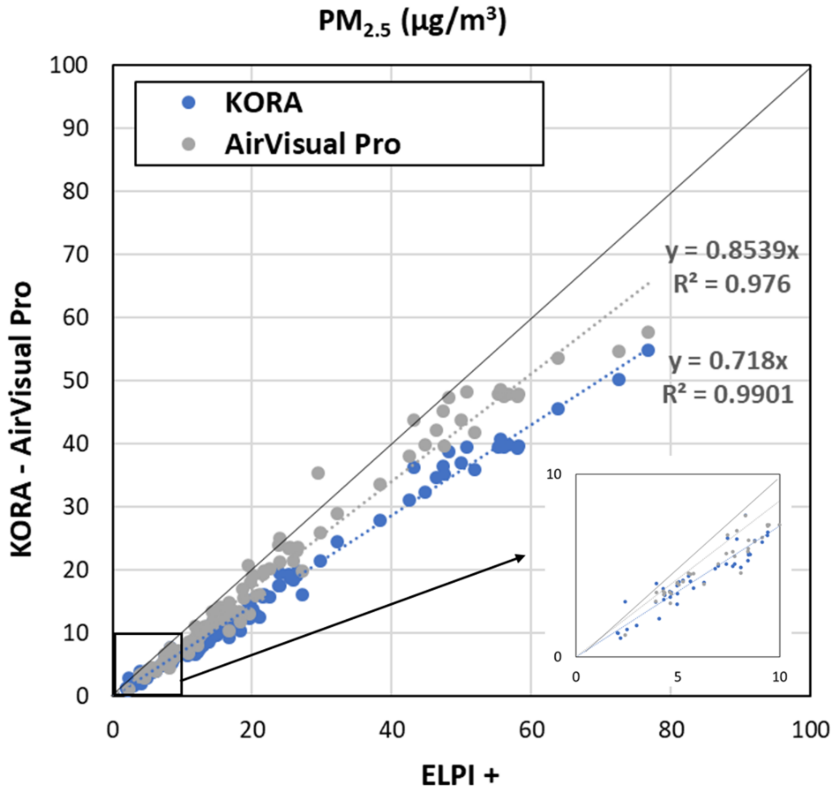
  • The underestimation of PM2.5 concentration indirectly calculated by low-cost optical sensors with respect to concentrations provided by the PMI, and the good alignment between the latter and the cascade impactor;
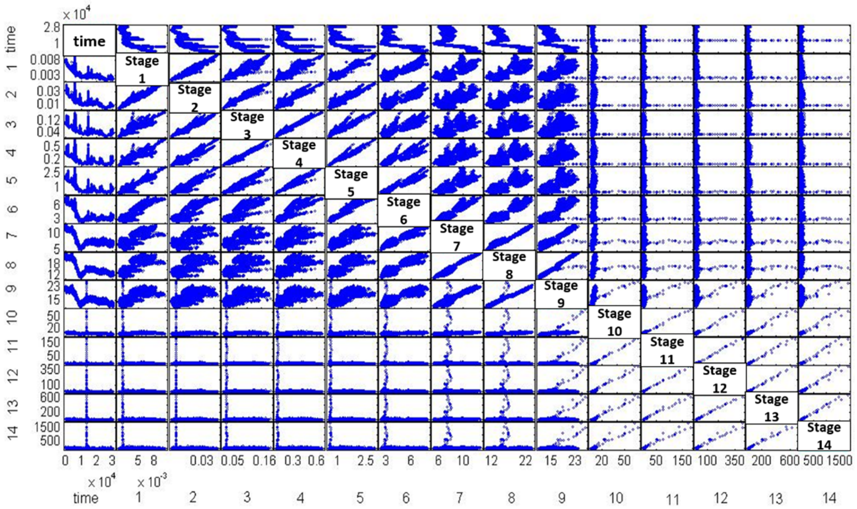
  • Different LODs for the optical sensor of the AirVisual Pro (250 nm) and KORA (380 nm) systems, estimated through the comparison with PM obtained by summing up size-segregated fractions of ELPI+ and supported by statistical analysis (PARAFAC model); and
  • An interesting correlation among size-segregated PM fractions measured by the cascade impactor (ELPI+) to discriminate specific emission sources indoors, in a confined environment, and outdoors.
In conclusion, the performance assessment of optical low-cost sensors showed the representativeness in providing a good evolution of concentrations over time and the cause–effect relationship between aerosol emission sources and their impact on air quality. Therefore, they can successfully be used to detect PM2.5 critical concentrations and eventual hot spots to drive local policies. Data analysis revealed the impossibility of discriminating aerosol emission sources and detecting particles in the ultrafine, and part of the fine, region. In order to use low-cost sensors for health impact assessments, the technology should be oriented toward the detection of particles comprising the nanoscale range.

Supplementary Materials

The following are available online at https://0-www-mdpi-com.brum.beds.ac.uk/article/10.3390/app11104360/s1, Table S1: Classification of the type of events occurred during the monitoring campaign with specific brief descriptions and labels; Table S2: Results of the least square method applied to the comparison of KORA and AirVisual Pro with the sum of various ELPI + fractions: 8–11, 7–11, 6–11, 1–11. The sum of the squares of deviations for each comparison is reported from columns 3 to 5, minimum values are in bold; Table S3: Correlation matrices of PN concentrations associated to ELPI + Stages from 1 to 14. High correlation is highlighted for coefficients larger than 0.7, reported in bold; Figure S1: Calendar of sampling days during March 2018; Figure S2: Daily concentrations of PM2.5 (averaged over 1 min sampling time) of KORA and AirVisual Pro collected outdoor (left) and in the garage (right). The starting time of different events is labelled with the corresponding letter as specified in Table S1; Figure S3: Daily concentrations of PM2.5 (averaged over 1 min sampling time) of KORA and AirVisual Pro collected in the warehouse. It should be noted the different y-axis scale up to 20 µg/m3 for “indoor quiet” and up to 45 µg/m3 for “indoor busy”. The starting time of different events is labelled with the corresponding letter as specified in Table S1; Figure S4: Daily PM2.5 concentrations (averaged over 1 min sampling time) of ELPI+ data from Stage 2, Stage 3, Stage 8 and Stage 11; Figure S5: Daily concentrations pattern measured by ELPI + Stage 4 (grey) and the corresponding linear correlation plots with Stages from 1 to 6. Data highlighted in black refer to the event of truck entering the warehouse; Figure S6: Altman Plots representing the difference of PM2.5 hourly concentrations between ELPI + and KORA(a), ELPI + and AirVisual Pro (b) and AirVisual Pro and KORA (c) measurements. On the y-axis the difference for each measure i of PM2.5 (di: ELPI + -KORA; ELPI + -AirVisual Pro; AirVisual Pro-KORA) between the 2 monitoring devices is plotted. On the x-axis the average value Xi,mean between the two monitoring devices considered is represented. The dashed line represents the di,mean while the two solid lines underline the 95% confidence interval (di,mean ± 1.96 SD); Figure S7: Score plots of the first two components (PC1 vs PC2) of the PCA, for each daily dataset; Figure S8: Score plot of the first two factors (F1 vs F2), for the first mode (instruments mode), of the PARAFAC statistical model.

Author Contributions

Conceptualization, L.B. and M.C.; methodology, L.B. and M.C.; software, F.K., A.A., A.W.M., L.B., M.C., S.F. and C.M.; validation, L.B. and M.C.; formal analysis, F.K., L.B. and M.C.; investigation, F.K and L.B.; resources, L.B., E.B., L.E.D., M.C., R.L., D.P., M.V., C.C., E.C., D.Z. and G.G.; data curation, L.B. and M.C.; writing—original draft preparation, L.B.; writing—review and editing, L.B., M.C., D.P., R.L., E.B., L.E.D., M.V., C.C., D.Z., E.C., A.F., G.G., S.F., A.W.M., C.M. and A.A.; visualization, L.B., M.C. and C.M.; supervision, L.B.; project administration, L.B.; funding acquisition, L.E.D., G.G. and R.L. All authors have read and agreed to the published version of the manuscript.

Funding

This work was funded by research from the National Institute of Health: R01ES019222-06A1, R56ES019222, P30ES023515; the European Union Sixth Framework Program: FOODCT-2006-016253; University of Brescia, Italy: UNBSCLE 9015; and B + Labnet University of Brescia (Brave Project). Its contents are under the responsibility of the authors and do not necessarily represent the official views of the funders.

Institutional Review Board Statement

Not applicable.

Informed Consent Statement

Not applicable.

Data Availability Statement

Data available on request due to restrictions. The data presented in this study are available on request from the corresponding author. The data are not publicly available due to privacy.

Conflicts of Interest

The authors declare no conflict of interest.

References

  1. UNION, PEAN. Directive 2008/50/EC of the European Parliament and the Council of 21 May 2008 on ambient air quality and cleaner air for Europe. Off. J. Eur. Union 2008, L 152, 1–44. [Google Scholar]
  2. Nidzgorska-Lencewicz, J.; Czarnecka, M. Thermal inversion and particulate matter concentration in Wrocław in winter season. Atmosphere 2020, 11, 1351. [Google Scholar] [CrossRef]
  3. Pope, C.A., III; Douglas, W. Dockery Health effects of fine particulate air pollution: Lines that connect. J. Air Waste Manag. Assoc. 2006, 56, 707–708. [Google Scholar] [CrossRef]
  4. Raaschou-Nielsen, O.; Beelen, R.; Wang, M.; Hoek, G.; Andersen, Z.J.; Hoffmann, B.; Stafoggia, M.; Samoli, E.; Weinmayr, G.; Dimakopoulou, K.; et al. Particulate matter air pollution components and risk for lung cancer. Environ. Int. 2016, 87, 66–73. [Google Scholar] [CrossRef]
  5. Wu, S.; Ni, Y.; Li, H.; Pan, L.; Yang, D.; Baccarelli, A.A.; Deng, F.; Chen, Y.; Shima, M.; Guo, X. Short-term exposure to high ambient air pollution increases airway inflammation and respiratory symptoms in chronic obstructive pulmonary disease patients in Beijing, China. Environ. Int. 2016, 94, 76–82. [Google Scholar] [CrossRef] [PubMed]
  6. De Berardis, B.; Paoletti, L. La frazione fine del particolato aerodisperso: Un inquinante di crescente rilevanza ambientale e sanitaria. Metodologie di raccolta e caratterizzazione delle singole particelle. Ann. Ist. Super. Sanita 1999, 35, 449–459. [Google Scholar]
  7. Fu, P.; Guo, X.; Cheung, F.M.H.; Yung, K.K.L. The association between PM 2.5 exposure and neurological disorders: A systematic review and meta-analysis. Sci. Total Environ. 2019, 655, 1240–1248. [Google Scholar] [CrossRef] [PubMed]
  8. Kumar, P.; Robins, A.; Vardoulakis, S.; Britter, R. A review of the characteristics of nanoparticles in the urban atmosphere and the prospects for developing regulatory controls. Atmos. Environ. 2010, 44, 5035–5052. [Google Scholar] [CrossRef] [Green Version]
  9. Stölzel, M.; Breitner, S.; Cyrys, J.; Pitz, M.; Wölke, G.; Kreyling, W.; Heinrich, J.; Wichmann, H.E.; Peters, A. Daily mortality and particulate matter in different size classes in Erfurt, Germany. J. Expo. Sci. Environ. Epidemiol. 2007, 17, 458–467. [Google Scholar] [CrossRef] [Green Version]
  10. Franck, U.; Herbarth, O.; Wehner, B.; Wiedensohler, A.; Manjarrez, M. How do the indoor size distributions of airborne submicron and ultrafine particles in the absence of significant indoor sources depend on outdoor distributions? Indoor Air 2003, 13, 174–181. [Google Scholar] [CrossRef]
  11. Zhao, J.; Weinhold, K.; Merkel, M.; Kecorius, S.; Schmidt, A.; Schlecht, S.; Tuch, T.; Wehner, B.; Birmili, W.; Wiedensohler, A. Concept of high quality simultaneous measurements of the indoor and outdoor aerosol to determine the exposure to fine and ultrafine particles in private homes. Gefahrst. Reinhalt. Luft 2018, 78, 73–78. [Google Scholar]
  12. Chiesa, M.; Urgnani, R.; Marzuoli, R.; Finco, A.; Gerosa, G. Site- and house-specific and meteorological factors influencing exchange of particles between outdoor and indoor domestic environments. Build. Environ. 2019, 160. [Google Scholar] [CrossRef]
  13. Klepeis, N.E.; Nelson, W.C.; Ott, W.R.; Robinson, J.P.; Tsang, A.M.; Switzer, P.; Behar, J.V.; Hern, S.C.; Engelmann, W.H. The National Human Activity Pattern Survey (NHAPS): A resource for assessing exposure to environmental pollutants. J. Expo. Anal. Environ. Epidemiol. 2001, 11, 231–252. [Google Scholar] [CrossRef] [Green Version]
  14. Brasche, S.; Bischof, W. Daily time spent indoors in German homes—Baseline data for the assessment of indoor exposure of German occupants. Int. J. Hyg. Environ. Health 2005, 208, 247–253. [Google Scholar] [CrossRef]
  15. Hussein, T.; Alameer, A.; Jaghbeir, O.; Albeitshaweesh, K.; Malkawi, M.; Boor, B.E.; Koivisto, A.J.; Löndahl, J.; Alrifai, O.; Al-Hunaiti, A. Indoor particle concentrations, size distributions, and exposures in middle eastern microenvironments. Atmosphere 2020, 11, 41. [Google Scholar] [CrossRef] [Green Version]
  16. Amato, F.; Viana, M.; Richard, A.; Furger, M.; Prévôt, A.S.H.; Nava, S.; Lucarelli, F.; Bukowiecki, N.; Alastuey, A.; Reche, C.; et al. Size and time-resolved roadside enrichment of atmospheric particulate pollutants. Atmos. Chem. Phys. 2011, 11, 2917–2931. [Google Scholar] [CrossRef] [Green Version]
  17. Perrino, C. Atmospheric Particulate Matter. 2010. Available online: https://www.researchgate.net/publication/228652246_Atmospheric_particulate_matter#fullTextFileContent (accessed on 23 March 2021).
  18. Wei, M.; Xu, C.; Xu, X.; Zhu, C.; Li, J.; Lv, G. Size distribution of bioaerosols from biomass burning emissions: Characteristics of bacterial and fungal communities in submicron (PM1.0) and fine (PM2.5) particles. Ecotoxicol. Environ. Saf. 2019, 171, 37–46. [Google Scholar] [CrossRef]
  19. Jovašević-Stojanović, M.; Bartonova, A.; Topalović, D.; Lazović, I.; Pokrić, B.; Ristovski, Z. On the use of small and cheaper sensors and devices for indicative citizen-based monitoring of respirable particulate matter. Environ. Pollut. 2015, 206, 696–704. [Google Scholar] [CrossRef] [PubMed]
  20. Chong, C.Y.; Kumar, S.P. Sensor networks: Evolution, opportunities, and challenges. Proc. IEEE 2003, 91, 1247–1256. [Google Scholar] [CrossRef] [Green Version]
  21. Kumar, P.; Morawska, L.; Martani, C.; Biskos, G.; Neophytou, M.; Di Sabatino, S.; Bell, M.; Norford, L.; Britter, R. The rise of low-cost sensing for managing air pollution in cities. Environ. Int. 2015, 75, 199–205. [Google Scholar] [CrossRef] [Green Version]
  22. White, R.M.; Paprotny, I.; Doering, F.; Cascio, W.E.; Solomon, P.A.; Gundel, L.A. Sensors and “apps” for community-based: Atmospheric monitoring. Air Waste Manag. Assoc. 2012, 36–40. Available online: https://www.researchgate.net/publication/279606358_Sensors_and_'apps'_for_community-based_Atmospheric_monitoring#fullTextFileContent (accessed on 23 March 2021).
  23. Castell, N.; Dauge, F.R.; Schneider, P.; Vogt, M.; Lerner, U.; Fishbain, B.; Broday, D.; Bartonova, A. Can commercial low-cost sensor platforms contribute to air quality monitoring and exposure estimates? Environ. Int. 2017, 99, 293–302. [Google Scholar] [CrossRef]
  24. Colombi, C.; Angius, S.; Gianelle, V.; Lazzarini, M. Particulate matter concentrations, Physical characteristics and elemental composition in the Milan underground transport system. Atmos. Environ. 2013, 70, 166–178. [Google Scholar] [CrossRef]
  25. Crilley, L.R.; Shaw, M.; Pound, R.; Kramer, L.J.; Price, R.; Young, S.; Lewis, A.C.; Pope, F.D. Evaluation of a low-cost optical particle counter (Alphasense OPC-N2) for ambient air monitoring. Atmos. Meas. Tech. 2018, 11, 709–720. [Google Scholar] [CrossRef] [Green Version]
  26. Han, I.; Symanski, E.; Stock, T.H. Feasibility of using low-cost portable particle monitors for measurement of fine and coarse particulate matter in urban ambient air. J. Air Waste Manag. Assoc. 2017, 67, 330–340. [Google Scholar] [CrossRef] [Green Version]
  27. Wang, Y.; Li, J.; Jing, H.; Zhang, Q.; Jiang, J.; Biswas, P. Laboratory Evaluation and Calibration of Three Low-Cost Particle Sensors for Particulate Matter Measurement. Aerosol Sci. Technol. 2015, 49, 1063–1077. [Google Scholar] [CrossRef]
  28. Sousan, S.; Koehler, K.; Thomas, G.; Park, J.H.; Hillman, M.; Halterman, A.; Peters, T.M. Inter-comparison of low-cost sensors for measuring the mass concentration of occupational aerosols. Aerosol Sci. Technol. 2016, 50, 462–473. [Google Scholar] [CrossRef] [Green Version]
  29. Järvinen, A.; Aitomaa, M.; Rostedt, A.; Keskinen, J.; Yli-Ojanperä, J. Calibration of the new electrical low pressure impactor (ELPI+). J. Aerosol Sci. 2014, 69, 150–159. [Google Scholar] [CrossRef] [Green Version]
  30. Rai, A.C.; Kumar, P.; Pilla, F.; Skouloudis, A.N.; Di Sabatino, S.; Ratti, C.; Yasar, A.; Rickerby, D. End-user perspective of low-cost sensors for outdoor air pollution monitoring. Sci. Total Environ. 2017, 607–608, 691–705. [Google Scholar] [CrossRef] [Green Version]
  31. Snyder, E.G.; Watkins, T.H.; Solomon, P.A.; Thoma, E.D.; Williams, R.W.; Hagler, G.S.W.; Shelow, D.; Hindin, D.A.; Kilaru, V.J.; Preuss, P.W. The changing paradigm of air pollution monitoring. Environ. Sci. Technol. 2013, 47, 11369–11377. [Google Scholar] [CrossRef] [PubMed]
  32. Pernigotti, D.; Georgieva, E.; Thunis, P.; Bessagnet, B. Impact of meteorology on air quality modeling over the Po valley in northern Italy. Atmos. Environ. 2012, 51, 303–310. [Google Scholar] [CrossRef]
  33. AirVisual Pro: Smart Air Quality Monitor|IQAir. Available online: https://www.iqair.com/air-quality-monitors/airvisual-pro (accessed on 17 March 2021).
  34. Cohen, A.J.; Brauer, M.; Burnett, R.; Anderson, H.R.; Frostad, J.; Estep, K.; Balakrishnan, K.; Brunekreef, B.; Dandona, L.; Dandona, R.; et al. Estimates and 25-year trends of the global burden of disease attributable to ambient air pollution: An analysis of data from the Global Burden of Diseases Study 2015. Lancet 2017, 389, 1907–1918. [Google Scholar] [CrossRef] [Green Version]
  35. Bro, R. PARAFAC. Tutorial and applications. Chemom. Intell. Lab. Syst. 1997, 38, 149–171. [Google Scholar] [CrossRef]
  36. Andersson, C.A.; Bro, R. The N-way Toolbox for MATLAB. Chemom. Intell. Lab. Syst. 2000, 52, 1–4. [Google Scholar] [CrossRef]
  37. Aria|ARPA Lombardia. Available online: https://www.arpalombardia.it/Pages/Aria/Qualita-aria.aspx (accessed on 17 March 2021).
  38. Singh, V.; Sahu, S.K.; Kesarkar, A.P.; Biswal, A. Estimation of high resolution emissions from road transport sector in a megacity Delhi. Urban Climate 2018, 26, 109–120. [Google Scholar] [CrossRef]
  39. DECRETO LEGISLATIVO 155, GU Serie Generale n.216 del 15-09-2010—Suppl. Ordinario n. 217. 2010. Available online: https://www.gazzettaufficiale.it/eli/id/2010/09/15/010G0177/sg (accessed on 23 March 2021).
  40. Abdel-Shafy, H.I.; Mansour, M.S.M. A review on polycyclic aromatic hydrocarbons: Source, environmental impact, effect on human health and remediation. Egypt. J. Pet. 2016, 25, 107–123. [Google Scholar] [CrossRef] [Green Version]
  41. Dorado, M.P.; Ballesteros, E.; Arnal, J.M.; Gómez, J.; López, F.J. Exhaust emissions from a Diesel engine fueled with transesterified waste olive oil. Fuel 2003, 82, 1311–1315. [Google Scholar] [CrossRef]
  42. Salo, L.; Mylläri, F.; Maasikmets, M.; Niemelä, V.; Konist, A.; Vainumäe, K.; Kupri, H.L.; Titova, R.; Simonen, P.; Aurela, M.; et al. Emission measurements with gravimetric impactors and electrical devices: An aerosol instrument comparison. Aerosol Sci. Technol. 2019, 53, 526–539. [Google Scholar] [CrossRef]
  43. Burkart, J.; Steiner, G.; Reischl, G.; Moshammer, H.; Neuberger, M.; Hitzenberger, R. Characterizing the performance of two optical particle counters (Grimm OPC1.108 and OPC1.109) under urban aerosol conditions. J. Aerosol Sci. 2010, 41, 953–962. [Google Scholar] [CrossRef] [Green Version]
  44. Giavarina, D. Understanding Bland Altman analysis. Biochem. Med. 2015, 25, 141–151. [Google Scholar] [CrossRef] [Green Version]
  45. Laucks, M.L. Aerosol Technology Properties, Behavior, and Measurement of Airborne Particles. J. Aerosol Sci. 2000, 31, 1121–1122. [Google Scholar] [CrossRef]
  46. Bro, R.; Kiers, H.A.L. A new efficient method for determining the number of components in PARAFAC models. J. Chemom. 2003, 17, 274–286. [Google Scholar] [CrossRef]
Figure 1. Pictures representing the sampling environments: (a) indoor, (b) outdoor, and (c) garage.
Applsci 11 04360 g001
Figure 2. Daily patterns of PM2.5 concentrations measured by KORA in different environments: (a) indoor busy, (b) indoor quiet, (c) outdoors, (d) garage, respectively. The labels (E: car exhausts, S: cigarette smoke, H: hammering works, C: crane movements, T: crane truck circulation, B: building and construction works, V: local forced ventilation, D: drilling work) describe the local ongoing activities (a complete list is given in Table S1).
Applsci 11 04360 g002
Figure 3. SEM images of the Teflon membrane filter where PM2.5 was collected at different magnifications.
Applsci 11 04360 g003
Figure 4. Linear correlation plots of PM concentrations (expressed in µg/m3) among all the ELPI+ fraction daily patterns derived from data monitored in the garage on 27 March 2018. Time as well as PM values associated with the ELPI+ stages (1–14) are reported on the x and y axis.
Applsci 11 04360 g004
Figure 5. Size distribution curves of normalized particle concentrations in different environmental conditions reported in terms of (a) number and (b) volume of particles (ELPI+ data). Specific expansions of the curves are shown in the insets.
Applsci 11 04360 g005
Figure 6. Hourly average concentrations of PM2.5 measured by KORA (blue circles) and AirVisual Pro (grey circles) with respect to ELPI+. Ideal correlation is shown by the slope 1 line. The inset better evidences the correlation at the lower end of concentration range.
Applsci 11 04360 g006
Figure 7. PM2.5 daily concentration patterns measured by AirVisual Pro, KORA, and ELPI+, the latter identified by the range of fractions (min–max) considered.
Applsci 11 04360 g007
Table 1. Cut-off particle size (D50%) of each impactor stage.
StageD50% (µm)
F0.006
20.016
30.0309
40.0547
50.0951
60.155
70.256
80.382
90.603
100.948
111.63
122.47
133.66
145.37
Table 2. PM2.5 total mass (expressed in µg) calculated for the ELPI+ andPMI. Relative percent errors (%) are reported in round brackets.
Monitoring Site, Date, and Environmental ConditionSampling Device(PM2.5) Total Mass (μg)
Outdoor 26 March 2018ELPI267 (1)
PMI250 (2)
Garage 27 March 2018ELPI277 (1)
PMI270 (2)
Table 3. PM2.5 daily minimum, maximum, and average concentrations measured by real-time sampling devices. Minimum and maximum concentrations, and the relative percent error (RE%) are also reported.
Monitoring Site, Date, and Environmental ConditionSampling DeviceRE%PM2.5 Daily Concentrations (μg/m3)
AVERAGEMINMAX
Indoor quiet 12 March 2018AirVisual Pro13.03.81.06.0
KORA1.43.61.99.7
ELPI+ 1.04.91.715.6
Indoor quiet 13 March 2018AirVisual Pro7.66.63.012.0
KORA0.95.93.79.5
ELPI+1.09.00.0000426.2
Indoor quiet 14 March 2018AirVisual Pro5.59.15.015.0
KORA0.68.04.312.2
ELPI+ 1.011.70.121.7
Indoor busy 15 March 2018AirVisual Pro2.619.47.046.0
KORA0.414.16.526.1
ELPI+ 1.019.80.000343.5
Indoor busy 16 March 2018AirVisual Pro5.88.63.020.0
KORA0.67.93.819.5
ELPI+ 1.0100.343
Indoor quiet 19 March 2018AirVisual Pro11.04.51.011.0
KORA1.14.60.79.9
ELPI+ 1.05.30.000314.6
Indoor busy 20 March 2018AirVisual Pro3.116.34.029.0
KORA0.413.45.821.7
ELPI+ 1.019.80.000351.3
Indoor busy 21 March 2018AirVisual Pro3.315.29.029.0
KORA0.412.58.624.1
ELPI+ 1.018.90.000349.0
Indoor quiet 22 March 2018AirVisualPro2.123.311.043.0
KORA0.319.710.237.3
ELPI+ 1.026.80.000348.0
Indoor busy 23 March 2018AirVisual Pro4.610.82.016.0
KORA0.68.76.315.2
ELPI+1.013.40.00722.8
Outdoors 26 March 2018AirVisual Pro1.145.213.0197.6
KORA0.138.532.881.9
ELPI+ 1.054.438.8454.4
Garage 27 March 2018AirVisual Pro1.147.334.078.3
KORA0.139.029.864.4
ELPI+ 1.051.135.5301.7
Table 4. Loss function values relative to the value for a one-component model, explained variance (expressed as percentage), and core consistency with respect to the number of components calculated by the PARAFAC model.
ComponentsLoss% Explained VarianceCore Consistency
11.0066.15100
20.5681.17100
30.3089.727.65
40.2192.8917.99
Publisher’s Note: MDPI stays neutral with regard to jurisdictional claims in published maps and institutional affiliations.

