Traffic State Prediction Using One-Dimensional Convolution Neural Networks and Long Short-Term Memory

Abstract

Traffic prediction is a vitally important keystone of an intelligent transportation system (ITS). It aims to improve travel route selection, reduce overall carbon emissions, mitigate congestion, and enhance safety. However, efficiently modelling traffic flow is challenging due to its dynamic and non-linear behaviour. With the availability of a vast number of data samples, deep neural network-based models are best suited to solve these challenges. However, conventional network-based models lack robustness and accuracy because of their incapability to capture traffic’s spatial and temporal correlations. Besides, they usually require data from adjacent roads to achieve accurate predictions. Hence, this article presents a one-dimensional (1D) convolution neural network (CNN) and long short-term memory (LSTM)-based traffic state prediction model, which was evaluated using the Zenodo and PeMS datasets. The model used three stacked layers of 1D CNN, and LSTM with a logarithmic hyperbolic cosine loss function. The 1D CNN layers extract the features from the data, and the goodness of the LSTM is used to remember the past events to leverage them for the learnt features for traffic state prediction. A comparative performance analysis of the proposed model against support vector regression, standard LSTM, gated recurrent units (GRUs), and CNN and GRU-based models under the same conditions is also presented. The results demonstrate very encouraging performance of the proposed model, improving the mean absolute error, root mean squared error, mean percentage absolute error, and coefficient of determination scores by a mean of 16.97%, 52.1%, 54.15%, and 7.87%, respectively, relative to the baselines under comparison.

1. Introduction

Traffic state prediction is a crucial component of an intelligent transportation system (ITS), which facilitates vehicle mobility, reduction of traffic congestion, and boosting of the economy. The transportation sector of developed countries accounts for 6 to 25% of their gross domestic products (GDP). On a macroeconomic level for advanced economies, it can account for up to half of their GDP [1]. These figures reflect the importance of efficient ITS implementation, which motivated the current research study.

Here, the traffic state prediction problem is modelled as a time series problem, where the prediction of future traffic states depends on previous traffic state data, such as speed and flow from an observed road section at different periods. Numerous previously suggested approaches have shown potential to solve this problem. Data-driven strategies are the most commonly employed techniques to address it because of their capabilities for dealing with complicated route layouts and the non-linearity of traffic flow [2]. However, corrupted and missing data samples pose difficulties in getting good estimation results using these approaches. A model that quickly and efficiently acquires the hidden features and spatio-temporal correlations in the data can have excellent performance. Additionally, the prediction of future states is always dependent on the previous states. Hence, the long short-term memory (LSTM) and gated recurrent unit (GRU) models, because of their worthiness in handling sequential information flows and internal memory, are remarkably suited to overcome these difficulties [3].

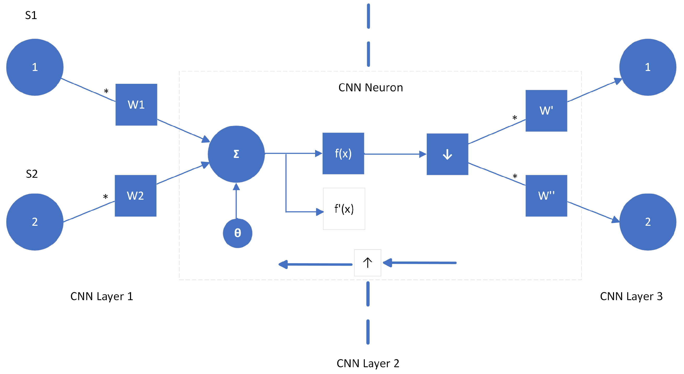
Convolution neural networks (CNNs), which are state-of-the-art, for example, in image processing and very efficient in extracting hidden features from input data, could be further combined with LSTM or GRU models in order to enhance the performance of the traffic state prediction system. However, traffic state data is one dimensional (1D) in nature, instead of an image that is two (or three) dimensional, making it difficult to apply to a CNN. The solution is 1D-CNN, where the kernel moves in one direction and can be used to extract features from the traffic state data, as can be seen in Figure 1.

In [4,5,6], CNN- and LSTM-based models were proposed to solve traffic state prediction problems. In [4], a deep temporal convolution network using residual connections for short-term traffic flow forecasting tasks was presented. The authors introduced a hierarchical temporal convolutional filter structure to capture the long-range dependencies using one-year-long datasets from road side units (RSUs) in the United Kingdom (https://webtris.highwaysengland.co.uk/ (accessed on 13 April 2022)) and achieved a mean absolute error (MAE) of $8.425$. In [5], a combined CNN and LSTM architecture was proposed for multi-lane traffic state prediction for the PeMS datasets (https://pems.dot.ca.gov/, Caltrans Performance Measurement System (PeMS) accessed on 13 April 2022)) by applying multiple features, mainly average speed and flow, for traffic state characterisation and by considering routing information, which led to an average MAE of $6.732$ and $1.475$ for flow and speed prediction, respectively. On the other hand, in [6], a vector auto-regression model was used prior to the CNN-LSTM architecture in order to capture the intrinsic association between different traffic variables. Based on the Yanan urban expressway and Shanghai datasets [7], the results led to an MAE of only $0.396$.

The current study proposes a model that differs from the aforementioned models in terms of architecture: three cells of stacked 1D-CNN and 1D-MaxPooling layers are applied to capture the hidden features, and three LSTM cells are used for predicting future traffic states taking into account the mean squared logarithmic error as the loss function. The three 1D-CNN layers include 32, 16, and 8 filters and pooling layers, with a pool size of two each. Three LSTM layers with the dimensionality of the output space of 256, 128, and 64, respectively, are used to leverage the learnt features from the CNN layers. After that, four fully connected dense layers act as the output layer, and three dropout layers show their worthiness in predicting the future traffic states. The proposed model demonstrated encouraging results relative to support vector regression (SVR), standard LSTM and GRU, and CNN–GRU-based models because of its architecture, optimisation approaches, and loss function. The main contributions of the proposed model are:

• It includes three stacked 1D-CNN and 1D-MaxPooling layers with the leaky rectified linear unit activation function to determine the hidden features of the traffic states and three LSTMs with recurrent kernel networks for prediction purposes.
• Its logarithmic hyperbolic cosine function, instead of conventional loss functions, demonstrated its worthiness in improving estimations to a good extent.
• It also demonstrates the requirement of a significant volume of data samples to more effectively capture the long-term dependencies within traffic states, and it effectively predicted over a longer time horizon than the baselines under comparison.

The remainder of this article is organised as follows: Section 2 presents the summary of state-of-the-art related works along with the identification of their limitations and future scopes; Section 3 depicts the formulations of the 1D-CNN combined with LSTM model; Section 4 covers the experimental setups and obtained results; Section 5 contains the description of the overall model’s performance and its feasibility in traffic state prediction; and, finally, Section 6 draws the conclusions and identifies possible future work.

2. Related Works

In a 2D-CNN, both the kernels and feature maps are 2D matrices. Whereas, in the case of a 1D-CNN, 1D arrays take their places. Another significant difference is that a 1D-CNN combines the feature extraction and classification tasks into one process. These two critical properties make the 1D-CNN model particularly suitable for dealing with 1D data samples. This section summarises relevant state-of-the-art works on LSTM, GRU, and CNN-based traffic state prediction models. It also identifies their limitations, future potential, and relationship with the proposed model.

2.1. Long Short-Term Memory

The LSTM model possesses a unique architecture to control the update process of its memory state using a gating mechanism, which is capable of counteracting the vanishing gradient problems of traditional recurrent neural networks (RNNs) [8,9]. As for LSTM-based models, the prediction always depends on the previous data samples, and so, missing or corrupted data samples significantly affect the performance of the models. Hence, dealing with this problem of missing or corrupted data is crucial for such models. Researchers use different approaches to address this problem. For example, the masking and imputation strategies proposed by [10] exhibited excellent outcomes. The proposed model obtained a mean absolute percentage error (MAPE) of only $2.10$% in hourly traffic volume and average annual daily traffic (AADT) forecasting tasks. Although the results demonstrated a remarkable improvement, the model suffers from a lack of robustness due to the occurrence of non-recurrent events.

Taking into account weather data and information about adjacent road segments is a very well-established solution to overcome the aforementioned problem. In [11], both rainfall and speed data were used to feed an LSTM model for traffic speed forecasting, which led to an enhancement both in terms of robustness and accuracy. The Bi-LSTM architecture proposed in [12], which considers the influence of air pollution, weather conditions, and temporal features of traffic states, also led to a more robust prediction model, which achieved a $1.02$% MAPE improvement relative to a CNN-based baseline.

Capturing both the spatial and temporal correlations of traffic states also plays a vital role in enhancing the robustness of a traffic prediction model. In [13], a capsule neural network (CapsNet) based on a CNN was used to obtain the spatial correlations, and a nested LSTM structure was employed to capture the temporal dependencies of the traffic states in order to effectively increase both the robustness and accuracy of the traffic estimations. The proposed solution achieved a MAPE of only $0.211$ for traffic speed prediction over a 20 min time horizon on a dataset from Gaode Maps (https://ditu.amap.com/ accessed on 13 April 2022). A recent study also suggested that the elimination of non-Gaussian disturbances can effectively boost the robustness of an LSTM model [14].

2.2. Gated Recurrent Unit

The literature also suggests the use of GRUs in traffic state prediction. Traditional RNNs are challenging to train, and for LSTMs, their training is even more challenging because of their complex architecture. However, GRUs exhibit their goodness in facilitating the training process [15]. GRUs require fewer parameters for training, and, hence, demonstrate faster convergence [16,17] than LSTMs.

In [18], a data fusion method was suggested to fuse information from two separate datasets, and a GRU was employed for travel time prediction to increase estimation accuracy. In [19], the authors looked at the computational cost and the optimisation of the network structure and suggested three recurrent neural network models, with the GRU model outperforming the others by achieving a root mean squared error (RMSE) of 9.26%.

A macroscopic fundamental diagram (MFD) demonstrated its usefulness in capturing the macroscopic traffic features, i.e., division of neighbouring regions between expressways and highways for traffic speed prediction [20]. Instead of directly feeding traffic state data to the GRU networks, first, an MFD constructs the road network into a weighted graph based on similarities of traffic operation. Then, a spatio–temporal correlation coefficient helps measure the relationship between the subdivisions of the network and build a matrix of traffic speed data. Finally, the GRU networks are used to predict future traffic speed by processing this matrix. Using truck GPS data [21], the proposed approach enhanced performance compared to the standard GRU model, with a 43.9% improvement in MAPE.

The literature also includes the application of attention mechanisms in combination with GRUs for capturing both the temporal and local aspects of traffic states [22]. This helped effectively acquire long-range dependencies and enabled the GRUs to predict over a longer time horizon (1 h) with excellent results (MAE of 1.26).

2.3. Convolution Neural Network

A combination of CNN and LSTM or GRU models can also solve traffic state prediction problems. Based on taxi big data, in [23], a model using spatio–temporal trajectory topology for traffic congestion prediction was presented. They used CNN to extract the spatial characteristics, and the LSTM memory characteristics were employed to recover the temporal characteristics from the trajectory of traffic flow. The experimental results showed a 1–2% improvement over conventional state-of-the-art techniques. However, the achieved MAPE of 24.339% indicates that the proposed model failed to provide efficient prediction accuracy. Hence, the current study aims to improve the prediction performance by offering a new architecture without using trajectory topological map extraction.

A differential approach proposed to reconstruct unstable time series into stationary ones and then feed them to a CNN–LSTM-based model demonstrated increased traffic flow prediction accuracy. The proposed model exhibited a MAPE of 76.14% for a 60 min prediction horizon [24]. Although prediction over a more extended period is more challenging, the presented accuracy is lower than usual. Thus, the model proposed in this article intends to increase prediction accuracy by applying a different approach that does not require reconstruction of the time-series dataset.

For traffic congestion prediction, a combination of a CNN with a bi-directional LSTM exhibited its worthiness. The CNN and Bi-LSTM models captured the spatial and temporal features, respectively. The initial stage involves folding traffic speed data according to spatio–temporal characteristics and building a three-dimensional matrix for the final model’s input. Compared to traditional and state-of-the-art approaches, the results showed a higher prediction accuracy with a mean absolute error of 0.43 [25]. However, only the data of 30 weekdays was used, which resulted in a lack of robustness. Traffic patterns are entirely different on weekends and weekdays. Hence, a model trained only on weekday data always lacks robustness and efficiency. Therefore, the current study took into account both weekday and weekend data to address this drawback.

In [26], a non-linear and non-periodic traffic speed prediction model was proposed based on a CNN for recognising spatio–temporal patterns of possibly congested urban traffic, which improved the accuracy by up to 23.8% for specific road segments. A cone-shaped binary masking approach selected the relevant input features to achieve good results. However, the prediction was for a 20 min time horizon, and this study aimed to extend the prediction time horizon with excellent accuracy.

The use of an inception–CNN-based traffic speed prediction model, where asymmetric convolution kernels were used to extract spatio–temporal correlations by focusing on different time or space domains, also exhibited improvements in both robustness and accuracy [27]. Such an approach enhanced the model’s non-linear representability and achieved an MAE of 2.45 for 30 min time steps on the Yanan urban expressway, Shanghai datasets. However, it required 8.3 million parameters for training and achieved an MAE of 2.55 in prediction over a 60 min time horizon. This study aimed to achieve better MAE values with fewer parameters.

Hence, all the aforementioned models need performance improvement in terms of robustness and accuracy. Notably, for prediction over a longer time horizon, tremendous efforts are required to meet the expectations. Fortunately, this study shows that efficient prediction performance can be achieved even for a longer time horizon by combining a 1D-CNN with LSTMs without using additional weather or adjacent intersection information.

3. Methodology

This section presents the formulation of the proposed 1D-CNN and LSTM-based model.

3.1. One-Dimensional Convolution Neural Network

A 1D-CNN model is a modified version of the conventional CNN model. A recent study [28] suggests that 1D-CNNs are superior to traditional CNNs in dealing with 1D data. The followings are the main distinctions between a 1D-CNN versus conventional CNNs:

• Both kernels and feature maps are 1D arrays instead of 2D matrices;
• Both feature extraction and classification operations take place in one process;
• For a 2D-CNN, data of dimension $N\times N$ convolving with a $K\times K$ kernel will have a computational complexity of $O\left(N^2{K}^2\right)$, but for a 1D-CNN, it is only $O\left(NK\right)$.

In a 1D-CNN model, a hidden CNN layer first performs a series of convolution operations, then the activation function passes their summation, and finally, subsampling occurs, Figure 2.

3.1.1. Convolution Layer

Let’s suppose that the input to xth layer is a tensor of order 3 with dimension: $H^x\times W^x\times D^x$, where H, W, and D represent rows, columns, and channels of the layer, respectively. A convolution kernel layered on top of an input tensor at any spatial point eases the computation of the products of relevant components, and the summation of their products helps to obtain the convolution result at that particular location. The kernel moves from top to bottom or left to right to finish the one-dimensional convolution operation. Let us now consider the case where the stride is 1 (one) and there is no padding. As a result, output O (or $I^{x+1}$) is found in vector ${\mathbb{R}}^{H^{x+1}\times W^{x+1}\times D^x}$, where $H^{x+1}=H^x-H+1$, $W^{x+1}=W^x-W+1$, and $D^{x+1}=D$. The convolution technique can be mathematically written as:

$$O_{i^{x+1},j^{x+1},d}=\sum _{i=0}^H\sum _{j=0}^W\sum _{d^x=0}^{d^x}{f}_{i,j,d^x,d}\times I_{i^{x+1}+i,j^{x+1}+j,d^x}^x+B_t$$

(1)

where $B_t$ represents the bias term. Applying a bias term to a convolution process helps the output become positive at horizontal edges in one direction and negative in other areas.

3.1.2. Pooling Layer

Now, let’s consider xth layer, which is a pooling layer, and whose inputs form tensor $I^x$ of order 3 with $I^xϵ{\mathbb{R}}^{H^x\times W^x\times D^x}$. There are no parameters required for the pooling process. If H divides $H^x$ and W divides $W^x$, and the stride equals the pooling spatial extent, the pooling output (O or equivalently $I^{x+1}$) will be a tensor of order 3 and of size $H^{x+1}\times W^{x+1}\times D^{x+1}$:

$$H^{x+1}=\frac{H^x}{H},W^{x+1}=\frac{W^x}{W},D^{x+1}=D^x$$

(2)

A pooling layer works independently on each channel of $I^x$. The elements of the matrix of $H^x\times W^x$ get separated into $H^{x+1}\times W^{x+1}$ non-overlapping subregions inside each channel, with each subregion being $H\times W$ in size. The pooling operator then maps a subregion into a single integer. The pooling operator in MaxPooling maps a subregion to its maximum value, whereas the pooling operator in AveragePooling maps a subregion to its average value. In terms of precise math, one has:

$$O_{i^{x+1},j^{x+1},d}=\underset{0\le i<H,0\le j<W}{max}{I}_{i^{x+1}\times H+i,j^{x+1}\times W+j,d}^x$$

(3)

The pooling kernel size and stride were 2 × 2 and 1 (one), respectively. The dropout layers helped to improve the generalisation ability of the proposed model. It sets the weights related to a particular percentage—after several trial-error tests, the best results were obtained for the three dropout layers with a rate of 0.2, 0.1, and 0.1, respectively—of nodes in the network to 0 (zero). It also used three completely linked layers (dense layers) in type $I_1\times I_2$, where $I_1$ is the input tensor’s size, and $I_2$ is the output tensor’s size; $I_2$ was always an integer, even if $I_1$ was a triplet. Three LSTM layers with 256, 128, and 64 units (dimensionality of the output space) eased the use of the learnt features from the CNN.

3.2. Long Short-Term Memory

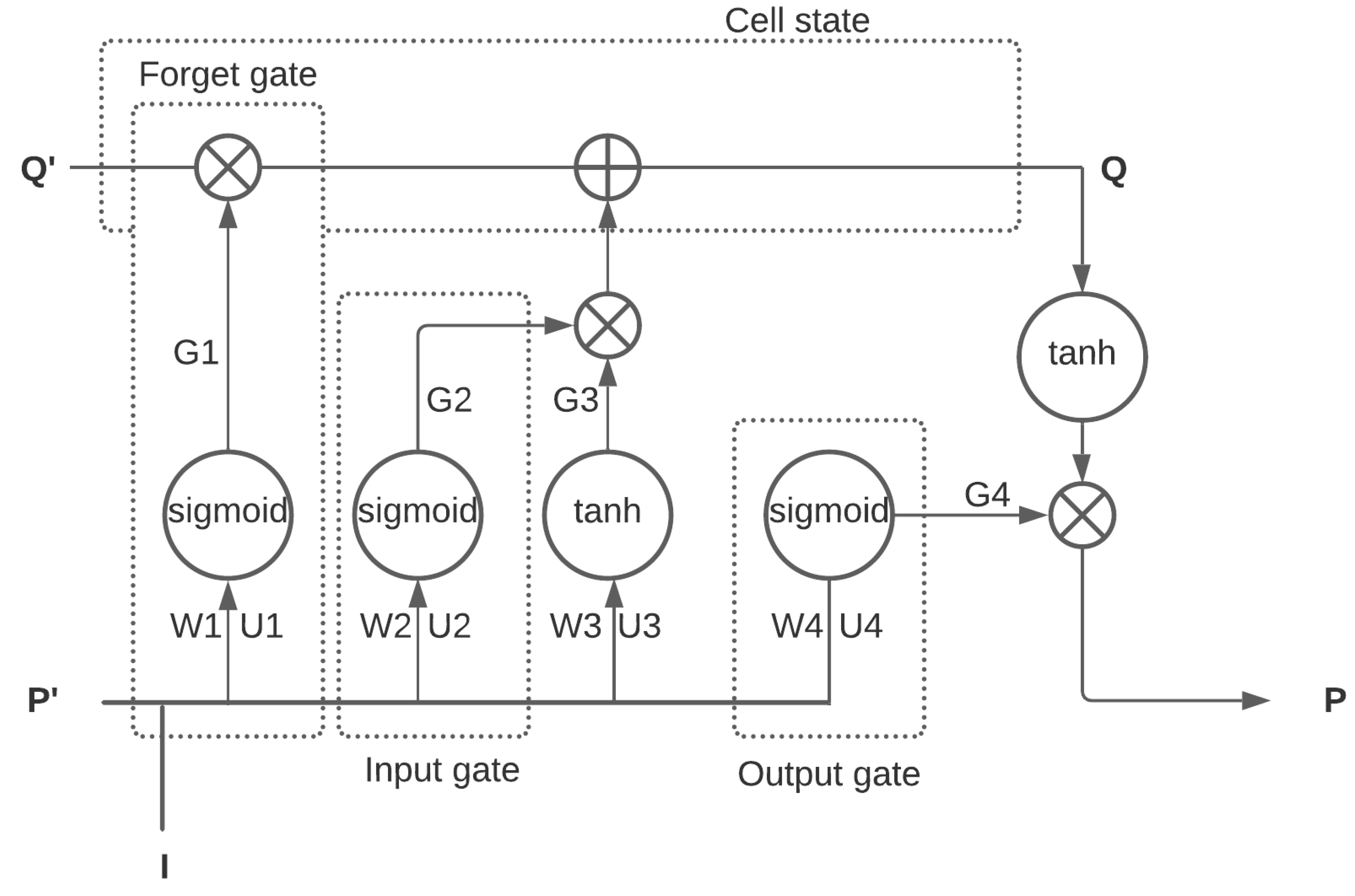
Figure 3 illustrates the internal architecture of the LSTM model. Let us assume that I, $P^{\prime }$, $Q^{\prime }$, Q, and P represent the input of the LSTM cell, output of the previous layer, input of the cell state, output of the cell state, and output of the LSTM cell, respectively. During forward propagation, the forget gate shown in the figure, which differentiates data that needs attention from those that can be overlooked, will calculate its output as:

$$G_1=sigmoid(I\times U_1+P^{\prime }\times W_1)$$

(4)

where $sigmoid$ is the activation function and $W_1$ and $U_1$ represent the corresponding weights of two inputs I and $P^{\prime }$, respectively. The reason behind the multiplication by $sigmoid$ is to set its output between 0 (zero) and 1 (one). Equations (5) and (6) define the working process of the input gate and have the power of setting up the values (setting values tending to 1 (one) in the memory and removing those tending towards −1) in the memory state. Multiplying by both the $sigmoid$ and $tanh$ functions facilitates this process:

$$G_2=sigmoid(I\times U_2+P^{\prime }\times W_2)$$

(5)

$$G_3=tanh(I\times U_3+P^{\prime }\times W_3)$$

(6)

Then, the output of memory state Q has the following form:

$$Q=Q^{\prime }\times G_1+G_2\times G_3$$

(7)

Similarly, Equation (8) governs the functionality of the output gate. The final output of LSTM cell P has the form:

$$G_4=sigmoid(I\times U_4+P^{\prime }\times W_4)$$

(8)

$$P=tanh\left(Q\right)\times G_4$$

(9)

The equations stated above govern the working principle of the LSTM cell during forward propagation. Now, during back propagation, which aims to tune the variables to reduce the errors, the LSTM model operates by calculating $\frac{\delta P}{\delta U_1}$, $\frac{\delta P}{\delta U_2}$, $\frac{\delta P}{\delta U_3}$, $\frac{\delta P}{\delta U_4}$, $\frac{\delta P}{\delta W_1}$, $\frac{\delta P}{\delta W_2}$, $\frac{\delta P}{\delta W_3}$, and $\frac{\delta P}{\delta W_4}$. Their subtraction from the old weights provides the final weights of the LSTM cell as:

$$W_{new}=W_{old}-\frac{\delta P}{\delta W}$$

(10)

$$U_{new}=U_{old}-\frac{\delta P}{\delta U}$$

(11)

3.3. Proposed Model

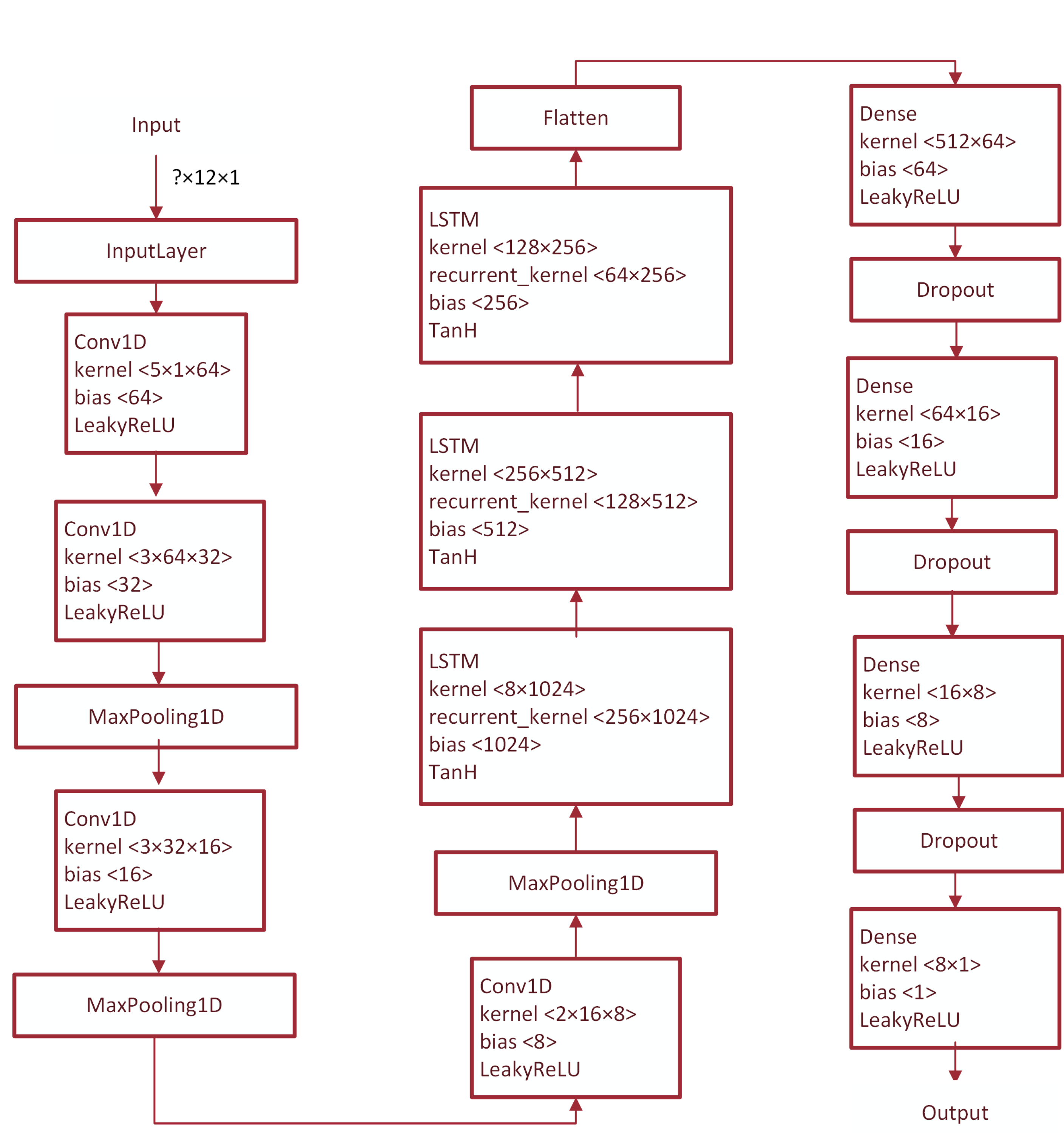
This study applied 1D-CNN and LSTM networks built according to previous formulations to learn the features from the input and predict future traffic speed and flow. The input layer received chunked single-length vectors from the raw data with 12 time steps, i.e., 60 min. A 1D-CNN with 64 filters and a kernel size of 5 acted as the input layer. Then, 3 stacked layers of CNN, each with a 1D-CNN with the leaky rectified linear unit (LeakyReLU) [30] as the activation function and a 1D MaxPooling layer were used to extract the data features. A stacked 3 LSTM layer processed these learnt features sequentially and, with the help of dense layers, predicted future traffic flow and speed. Figure 4 illustrates the architecture of the proposed model.

4. Experiments

The training of a 1D-CNN model requires low computational resources, and hence, a laptop computer (HP ZBook 15 Mobile Workstation) with an Intel^® Core™ i7-10750H processor at 2.6 GHz, 16 GB of RAM, without any graphical processing units (GPU), and Ubuntu as the operating system, was used to train the proposed model. The open-source TensorFlow machine learning library written in Python was used as a coding platform. Implementation consisted of four stages. The first stage chunked the data into training and test sets: 70% for training and the rest for testing, applied normalisation techniques from ‘sklearn.preprocessing’, and converted the training and test data into single-length vectors, each with a time step of 12. Defining the model took place in the second step. The TensorFlow ‘Sequential’ class and ‘keras.layers’ modules were used to build the model function. The third phase included defining the model training function. The TensorFlow ‘Model Training’ application programming interface (API) was employed to achieve this.

The mean squared logarithmic error function from ‘Keras Losses’ API and adaptive moment estimation (Adam) function from ‘Keras Optimizers’ API were used as the loss function and optimiser, respectively. The final phase evaluated the proposed model and plotted the obtained results. Two separate predefined functions helped with this. The ‘sklearn.metrics’ API eased import of the evaluation metrics, and ‘Matplotlib’ with ‘NumPy’ libraries helped to plot the results to allow graphical comparisons. The quantity of trainable parameters of the proposed model was 564,377, and it took 112 min to train it for 100 epochs. In this study, support vector regression, LSTM, gated recurrent unit, and CNN–GRU-based models were also trained in the same environment with identical parameters in order to make comprehensive comparisons. The total training time for the LSTM, GRU, and CNN–GRU models was 85, 78, and 108 min, respectively.

4.1. Evaluation Metrics

The state-of-the-art mean absolute percentage error, root mean squared error, mean absolute error, and coefficient of determination ($R^2$ score) were used to assess the accuracy of the proposed model. If r, p are the actual and predicted values, N is the number of samples, and $r_i$ and $p_i$ are values of the ith samples in r and p, respectively, then, their formulations have the following forms:

The average absolute percent error between the actual and predicted values determines the MAPE for each period [31]:

$$MAPE(r,p)=\frac{100\%}{N}\sum {i=1}^N\left|\frac{r_i-p_i}{r_i}\right|$$

(12)

The mean absolute error is simply an arithmetic average of the absolute errors:

$$MAE(r,p)=\frac{1}{N}\sum _{i=1}^N\left|p_i-r_i\right|$$

(13)

The root mean squared error is the standard deviation of the residuals, i.e., prediction errors; in mathematical form:

$$RMSE(r,p)=\sqrt{\frac{1}{N}\sum _{i=1}^N{(r_i-p_i)}^2}$$

(14)

Equation (15) presents the $R^2$ score that computes the coefficient of determination. The explained variance ratio indicates the model’s goodness of fit and thus, indicates how well the model would predict the unseen, i.e., missing, data samples:

$$R^2(r,p)=1-\frac{{\sum }_{i=1}^N{(r_i-p_i)}^2}{{\sum }_{i=1}^N{(r_i-{\overline{p}}_i)}^2}$$

(15)

where $\overline{p}$ represents the mean of the true values and is equal to $\frac{1}{N}{\sum }_{i=1}^N{r}_i$.

4.2. Datasets

Two publicly available state-of-the-art datasets for predicting traffic flow and speed were used in this study. The reason for selecting two different datasets was to make a natural generalisation, i.e., in order to demonstrate that the proposed model can perform well regardless of data attributes and source.

• The current study used the Caltrans’ Performance Measurement System (PeMS) database [32] that includes real-time traffic data acquired using 39,000 individual sensors. It covers the road networks of all of California’s main urban areas over a 10-year period. The dataset has 6 months of aggregated traffic flow data over a period of 5 min. Here, the data from the southern California region was used from 1 June 2021 to 15 December 2021, which includes 99,359 data samples.
• Additionally to PeMS, an urban traffic speed dataset from Guangzhou, China, which comprises 214 road segments mostly from urban expressways and arterials gathered at 10 min intervals from 1 August 2016 to 30 September 2016 [33] was used.

Data Analysis

Before applying the proposed model, the datasets needed to be analysed in order to carry out efficient predictions. This consisted of finding seasonality, trends, and residual characteristics.

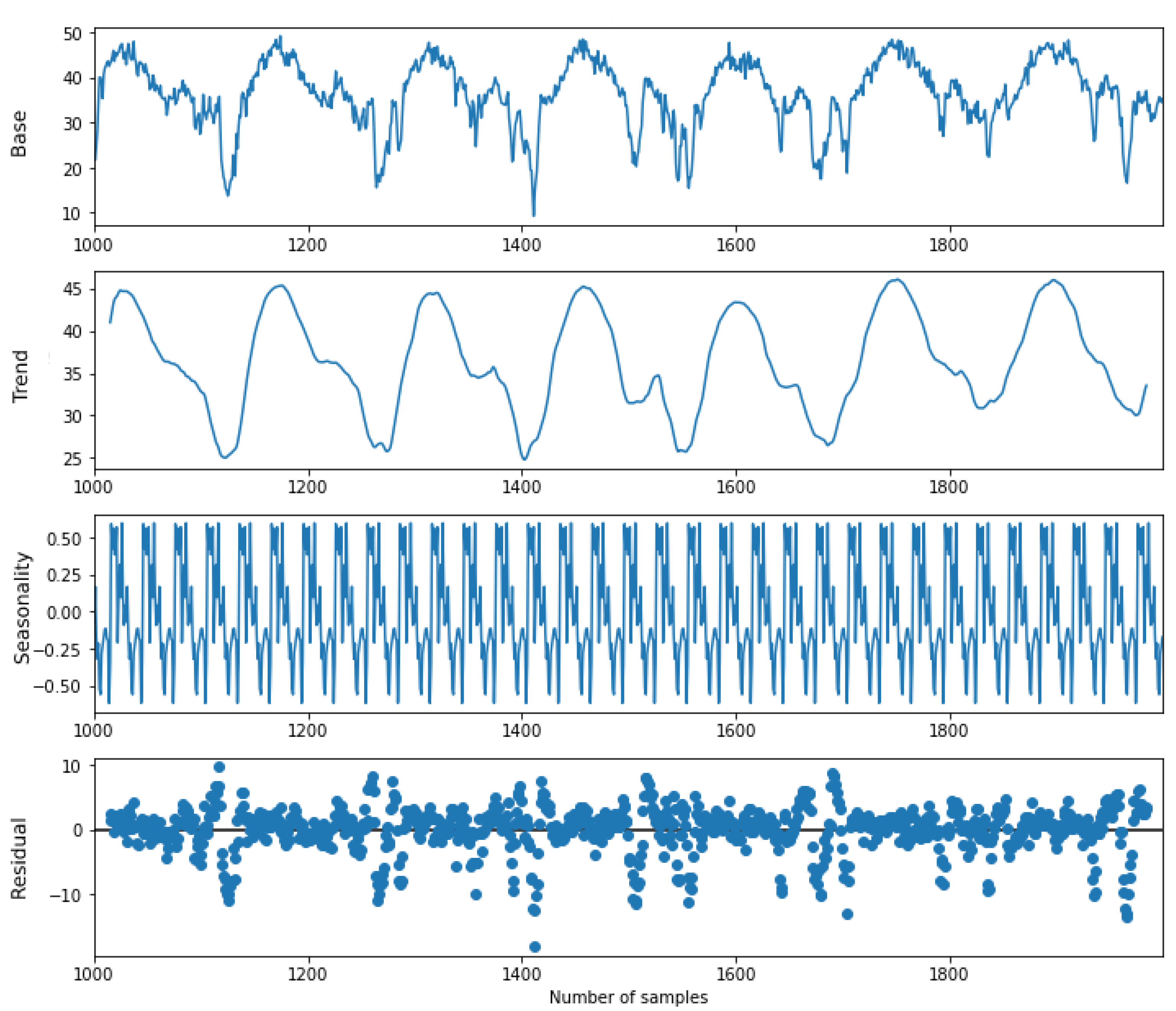
Trends show the general direction of data over an extended period, and the calculation of moving averages helps to define the long-term trend. On the other hand, seasonality illustrates repetitive trends over regular intervals. The third component is the residual, which corresponds to the differences between expected and actual values in terms of long-term trends and seasonal effects. The data amplitude was always proportional to its mean distribution, revealing the addictive nature of the used datasets. The additive decomposition approach was taken into account to depict these characteristics, as shown in Figure 5. In this figure, the first, second, third, and fourth panels from the top illustrate line-plots of the actual data, found trends, seasonality, and residual within the traffic speed dataset. The last plot shows that many data points do not match the expected values in terms of seasonality and trends.

If all of the data points of a residual plot lie near the 0 (zero) axis, it means the dataset is perfectly representable in terms of seasonality and trends. However, the current case shows the opposite scenario. Therefore, modelling these datasets is more challenging than modelling conventional time-series data. Directly feeding these data to the LSTM networks might cause inefficient learning. Hence, first, a CNN should be used to extract those features, and then LSTM networks should be employed to process them.

The determination of stationarity is another crucial aspect of traffic state data analysis. The Kwiatkowski–Phillips–Schmidt–Shin (KPSS) [34] test helped to determine the stationarity of the used datasets. The ‘statsmodels-0.14.0’ package was used as the platform for KPSS analysis, leading to the results indicated in

Table 1. Results of the KPSS test on traffic speed data.

Attributes	Values
Test Statistics	2.722
p-Value	0.01
Critical Values	(‘10%’: 0.119, ‘5%’: 0.146, ‘2.5%’: 0.176, ‘1%’: 0.216)

.

A critical value divides a graph into regions (for example, the rejection region). If the test value falls inside the rejection region, the null hypothesis is rejected. However, the stationarity of the raw data depends on the p-value: a value above 0.05 represents stationarity, otherwise the dataset has non-stationarity. Interestingly, the speed and flow data were non-stationary and stationary, respectively.

4.3. Data Preprocessing

The first 1D-CNN layer of the proposed model acts as the input layer to receive one-dimensional traffic state data. The data features must be on the same scale for efficient convolution operations. The normalisation techniques facilitate the task of converting differently scaled feature points into an identical scale, guaranteeing each feature bears equal importance. Different normalisation algorithms were tested, such as the MinMaxScaler, MaxAbsScaler, StandardScaler and RobustScaler algorithms. After several trial–error tests, it was found that the MaxAbsScaler algorithm led to the best results. Data preprocessing also included the formation of training and test datasets. The traffic speed and flow datasets contain 1,855,589 and 99,359 data samples, respectvely, with 70% of them constituting the training dataset and the rest used for testing. Data preprocessing also included the conversion of training and test data into single-length vectors, each with a time step of 12.

4.4. Training

For training the proposed model, it was found that the following hyper-parameters led to the best performance: $batch\_size=32$, $epochs=100$, $validation\_split$ = 0.05, $learning\_rate$ = $5\times {10}^{-4}$, $decay\_step$ = 100,000, $decay\_rate$ = 0.98, and $ϵ$ = $1\times {10}^{-7}$. The number of trainable parameters was 582,657. The logarithmic hyperbolic cosine error loss function [35] and adaptive moment estimation (Adam), a combination of gradient descent with momentum and root mean square propagation (RMSprop) algorithms [36], showed their worthiness to calculate the loss and optimisation for the gradient descent. Adam demonstrated its efficiency in dealing with several parameters using less memory. The number of output filters for the three 1D-CNN layers were 64, 32, and 16, respectively, whereas, for the three 1D MaxPooling layers, a pool size of two provided the best results.

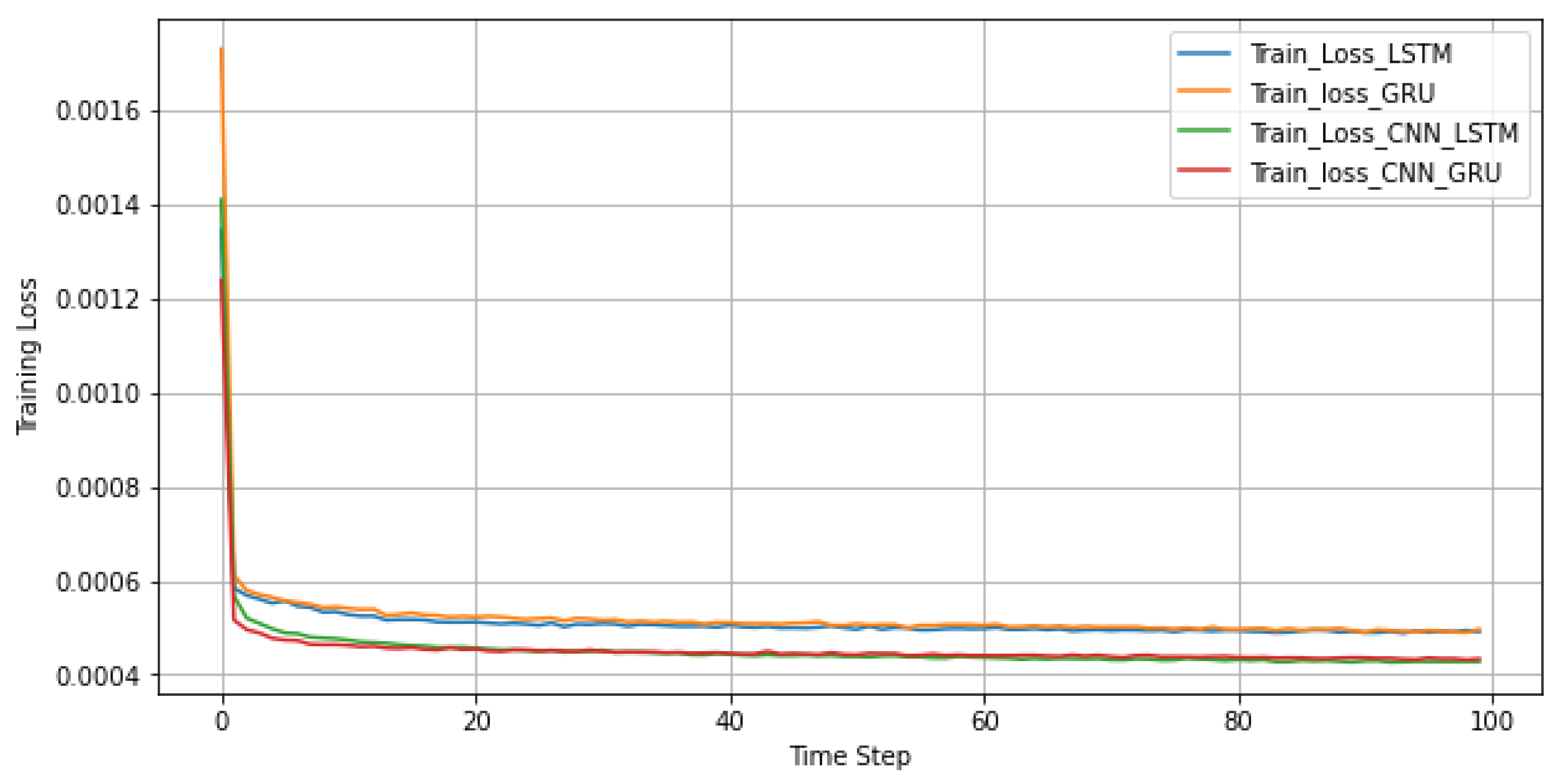
Figure 6 allows visual comparison of training loss among the different models under study. It shows that the proposed 1D-CNN–LSTM model and the other baselines under consideration are free of under-fitting and over-fitting issues and that the models accurately match the data.

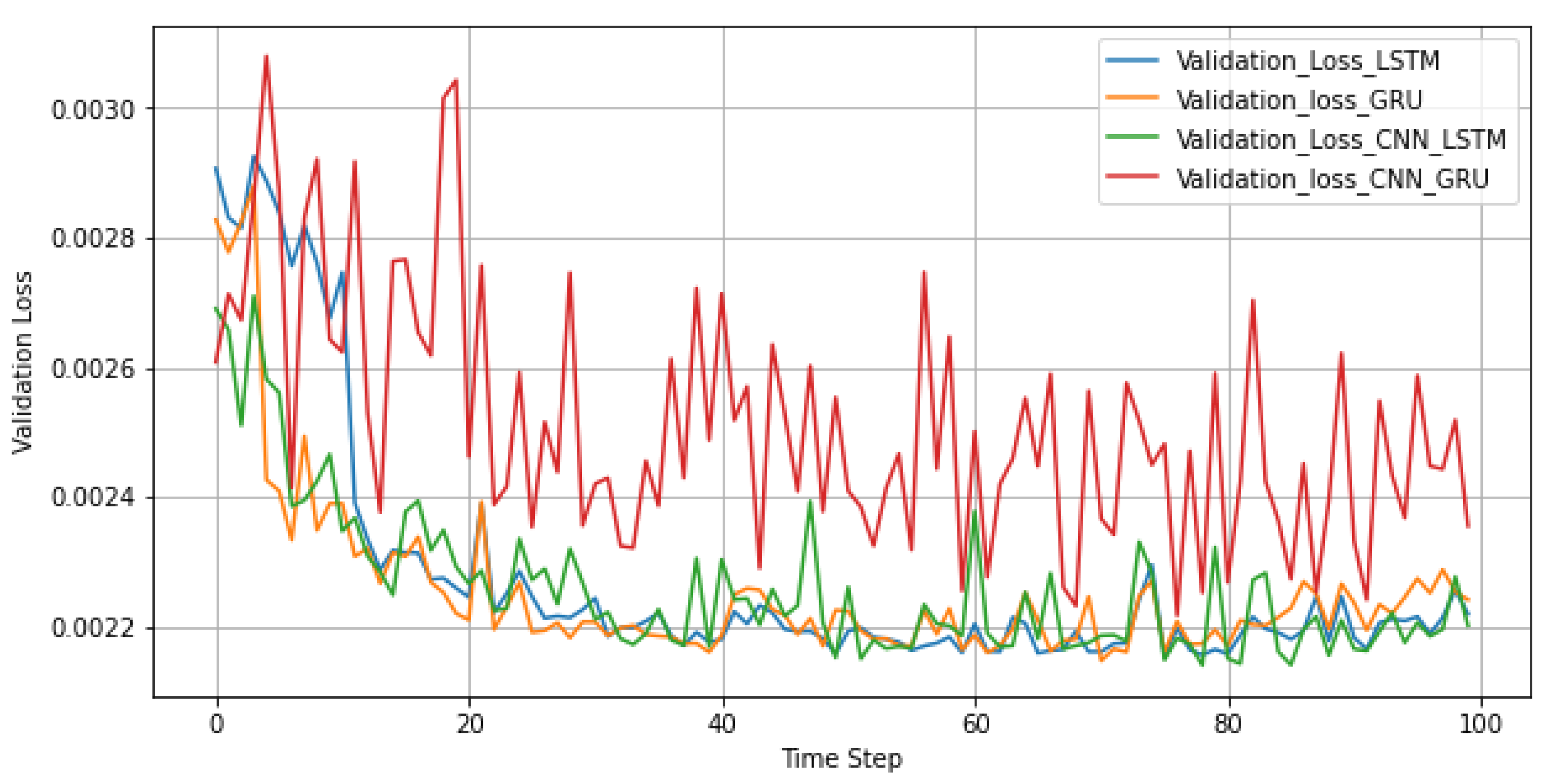
Figure 7 illustrates the validation loss comparison among the different models under study. It reveals that the proposed 1D-CNN–LSTM, GRU and LSTM models fit new data well. However, for the CNN–GRU-based model, the validation function moves noisily. The CNN–GRU model struggled to model these examples since the validation data did not represent the training data. On the other hand, the proposed CNN–LSTM model performed well even though the validation dataset is more challenging to predict than the training dataset.

4.5. Results

The proposed 1D-CNN–LSTM model showed tremendous improvements in terms of the used state-of-the-art metrics relative to the SVR, GRU, LSTM, and CNN–GRU models.

Table 2. Performance comparison of different models under study in terms of the used state-of-the-art metrics on the traffic flow dataset.

Metrics	SVR	LSTM	GRU	CNN–GRU	CNN–LSTM
MAPE	15.46%	12.45%	12.41%	14.45%	12.34% *
RMSE	$15.7$	$7.84$	$7.89$	$7.87$	$7.66$ *
MAE	$14.00$	$5.86$	$5.88$	$6.06$	$5.75$ *
$R^2$	$0.863$	$0.867$	$0.865$	$0.865$	$0.873$ *

Here, * represents the best-found result among the models under comparison.

confirms the awe-inspiring performance of the proposed model based on the MAPE, RMSE, MAE, and $R^2$ score. These values were obtained using the traffic flow dataset and based on the parameters described in Section 4.4 for prediction over a one-week time horizon.

Relative to the other baselines, the MAPE of 12.34% achieved by the proposed model is 0.6–20.1% less. On top of that, the proposed model exhibited 1.91–50.6% and 3.02–58.7% performance improvement in terms of RMSE and MAE, respectively, relative to the baselines under consideration. It also obtained an $R^2$ score of 0.873, which indicates that the model correctly predicted 87.3% of the unseen, i.e., missing, data samples.

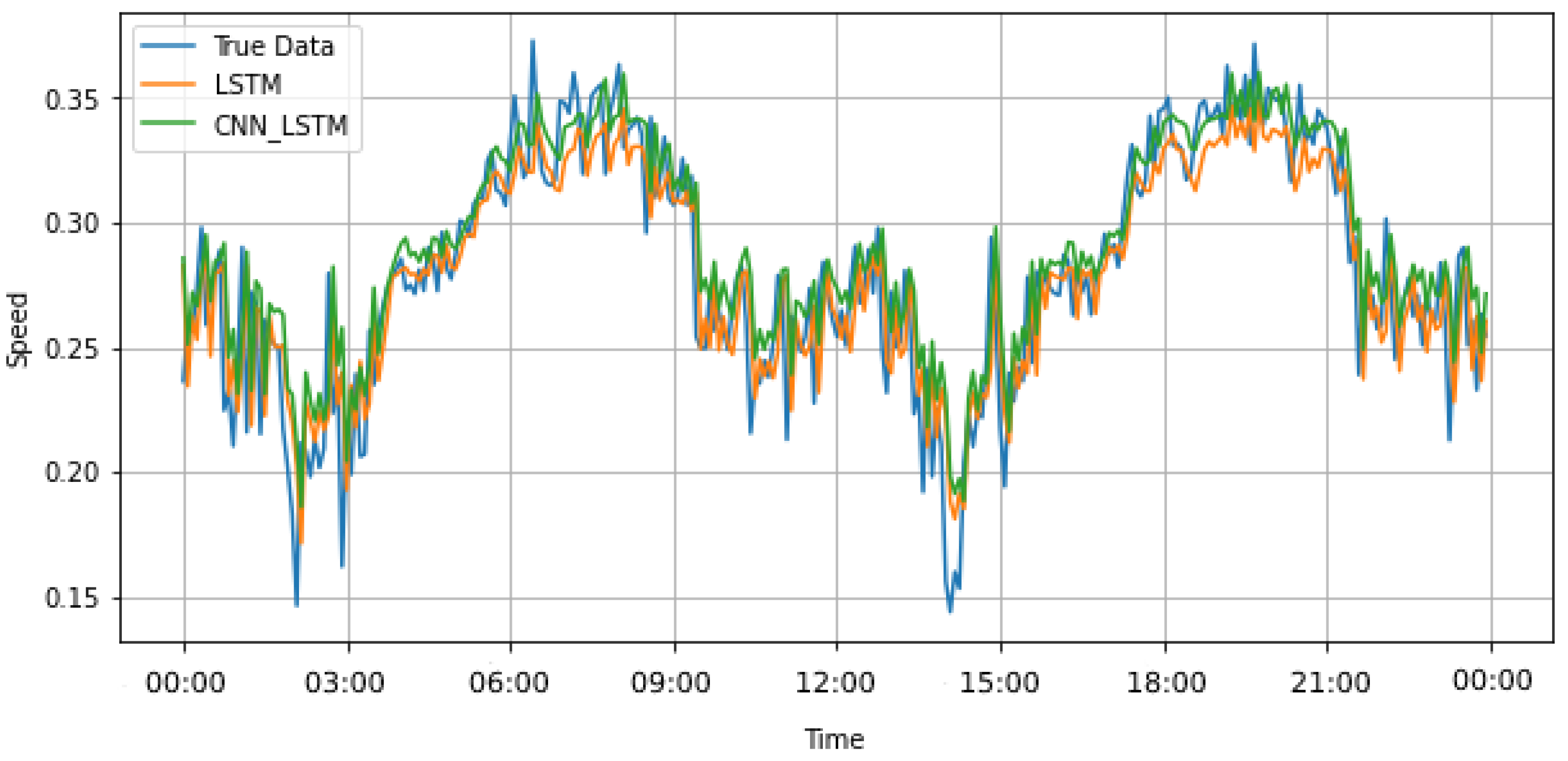
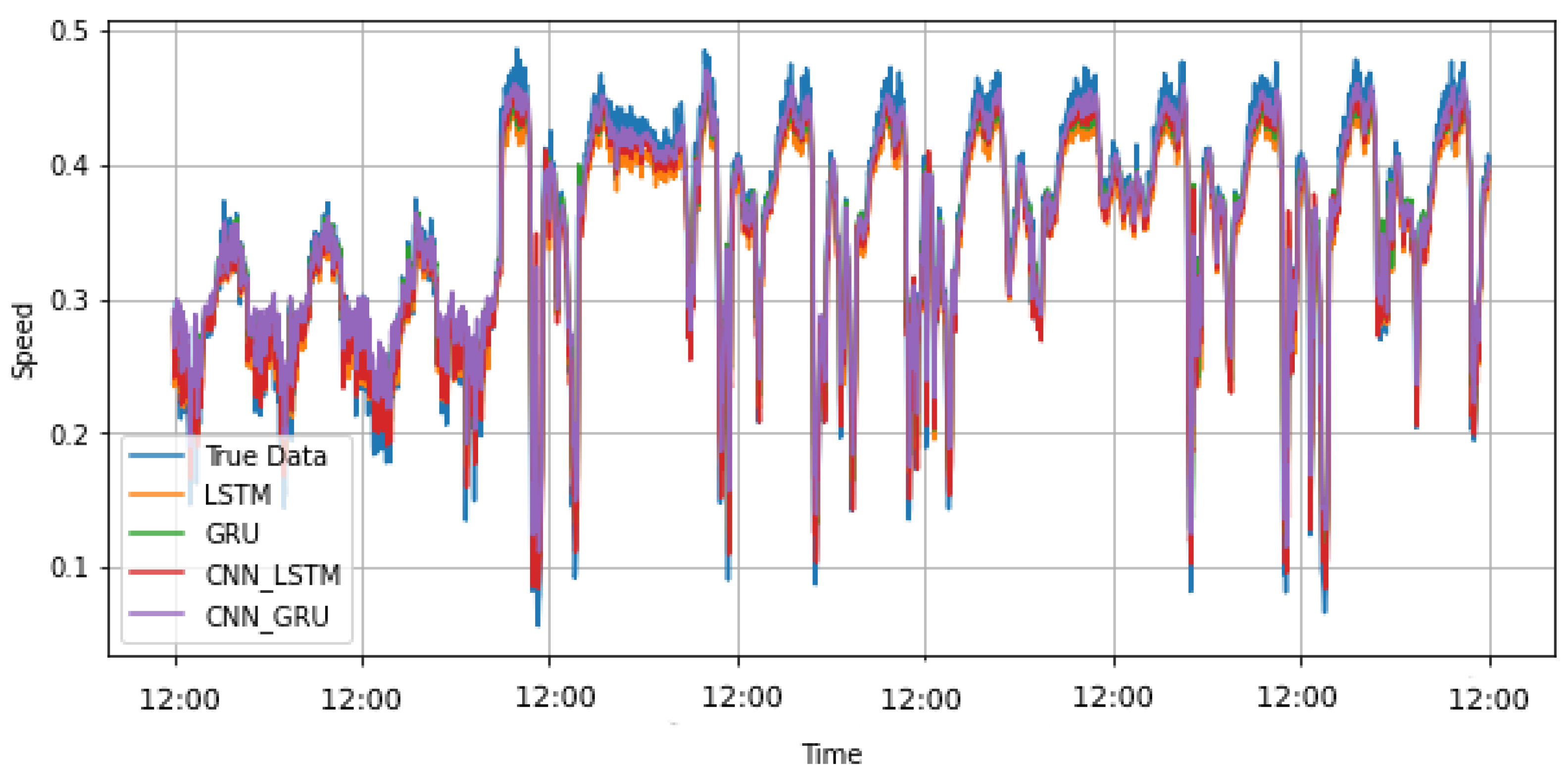
Figure 8 and Figure 9 allow visual comparison of the prediction performance of the models under study over 24 h and weekly horizons, respectively, for the traffic speed dataset. It is clear from the plots that the proposed model predicted traffic speed values more accurately than the other baselines. Another critical finding to notice from the included plots is the ability of the proposed model to effectively learn long-range data dependencies. Even for times periods greater than a week, the model can correctly predict traffic speed values.

Table 3. Performance comparison of the different models under study in terms of the used state-of-the-art metrics on the traffic speed dataset.

Metrics	SVR	LSTM	GRU	CNN–GRU	CNN–LSTM
MAPE	$9.30$%	$8.27$%	$8.31$%	$8.897$%	7.27% *
RMSE	$0.78$	$0.0291$	$0.0288$	$0.0295$	0.0266 *
MAE	$1.09$	$0.02178$	$0.02042$	$0.02061$	0.01896 *
$R^2$	$0.784$	$0.896$	$0.898$	$0.894$	0.913 *

Here, * represents the best found result among the models under comparison.

shows the performance of the proposed model on the traffic speed dataset. The logarithmic hyperbolic cosine (LogCosh) loss function provided these outcomes. Similar to the traffic flow dataset, these values were obtained based on the employed hyper-parameters described in Section 4.4 on a prediction over a one-week time horizon. The proposed model outperformed the other baselines under consideration in terms of all the used evaluation metrics. It exhibited MAPE, RMSE, MAE, and $R^2$ score improvements of 12.1–21.83%, 7.6–96.6%, 25.7–82.6%, and 1.64–14.1%, respectively.

5. Discussion

Traffic is highly dynamic, so building an efficient traffic prediction model is challenging. Further, the robustness of a model is greatly dependent on capturing both spatial and temporal features of traffic. For the SVR model, it was particularly challenging to capture those features because it is less capable of dealing with a vast amount of data and noisy data samples, specifically when overlapping of target classes occurs. The obtained experimental results demonstrate its incapability of dealing with these problems.

On the other hand, the LSTM and GRU models can remember relevant past information because of their memory characteristics. Hence, these models are suitable for time series prediction tasks. However, these models require feeding the data sequences directly to the input, and the path distances will always increase proportionally, which can cause inefficiency in capturing long-range correlation relationships.

On the contrary, convolution layers can learn the hidden features of data more effectively than the other baselines. Hence, instead of feeding data directly to the model, 1D convolution layers were used to extract features first, and then the goodness of the LSTM or GRU models was employed to process those learnt features sequence-by-sequence for prediction purposes. This technique demonstrated very encouraging performance improvements in terms of the used state-of-the-art metrics.

During the current study, different state-of-the-art techniques were assessed for data normalisation; mainly, MaxAbsScaler—scaling each feature by its maximum absolute value; MinMaxScaler—transforming features by scaling each feature to a given range 0, 1; RrobustSCaler—scaling features using statistics that are robust to outliers; and StandardScaler—standardise elements by removing the mean and scaling to unit variance. Interestingly, MaxAbsScaler and StandardScaler exhibited the best and most minor outcomes, respectively.

This study also assessed the Bi-Directional LSTM and GRU architecture instead of normal LSTM or GRU. Interestingly, in terms of the MAPE, the proposed model had a performance degradation of 60.9%. Moreover, batch normalisation layers, which are additional layers used to normalise the outputs of the first hidden layer before passing them on to the next hidden layer and aim to keep the network stable throughout training, were inserted into the proposed model. Further, the insertion of layer normalisation within the hidden layers was considered to predict the normalisation statistics from the aggregated inputs of the neurons and to resist any additional dependencies among the training samples. Both exhibited discouraging results, particularly the insertion of the normalisation layers. Although some previous research, for example [37], had opposite findings. However, in the current type of data, layer normalisation within a hidden layer failed to correctly predict the normalisation statistics from the aggregated inputs of the neurons.

In this study, the proposed model was trained for different combinations of 1D-CNN and LSTM layers using the same environment and identical hyper-parameters.

Table 4. Ablation studies of the proposed model on the traffic speed dataset.

1D-CNN Layers	LSTM Layers	Parameters	RMSE
5	5	599 K	$0.02919$
4	4	569 K	$0.02839$
3	3	562 K	0.0266 *
2	2	174 K	$0.863$

Here, * represents the best found result among the models under comparison.

indicates the performance of the proposed model in terms of different parameters. The number of used 1D-CNN or LSTM layers significantly affected the model’s performance. However, it was fascinating to observe that increasing the number of layers did not effectively enhance the outcome. It was found that the best RMSE of $0.024016$ was obtained for three stacked layers of 1D-CNN and LSTM networks.

The application of the loss function is vitally essential for a competent deep learning model. The influence of different loss functions was assessed on the proposed model’s performance. The Huber [38] and LogCosh loss functions demonstrated better performances relative to the mean squared error.

Table 5. MAE obtained by the models under study in terms of the used loss function on the traffic speed dataset.

Loss Function	LSTM	GRU	CNN–GRU	CNN–LSTM
MSE	$0.0229$ *	$0.0234$	$0.0245$	$0.024$
MAPE	$0.0293$	$0.0287$	$0.067$	$0.025$ *
LogCosh	$0.0218$	$0.0204$	$0.0206$	$0.019$ *

Here, * represents the best found result among the models under comparison.

presents the results of the performance comparison of the models under study in terms of MSE, MAPE, and LogCosh loss functions. In terms of statistics, the utilisation of LogCosh led to a 26.7% improvement relative to the MSE loss function with regard to the MAE.

Similarly, on the traffic flow data from the PeMS dataset, the LogCosh function provided the best output.

Table 6. MAE obtained by the models under study in terms of the used loss function on the traffic flow dataset.

Loss Function	LSTM	GRU	CNN–GRU	CNN–LSTM
MSE	$6.47$	$6.515$	6.44 *	$6.52$
MAPE	$6.39$	$6.9$	$7.1$	6.01 *
LogCosh	$5.86$	$5.88$	$6.06$	5.75 *

Here, * represents the best found result among the models under comparison.

presents the obtained MAE values by the different models under study using different loss functions. It was interesting to observe that CNN–GRU outperformed the proposed model while using the MSE as the loss function.

The number of trainable parameters of each baseline under consideration, i.e., of the LSTM, GRU, and CNN–GRU models, were equal to 516 K, 389 K, and 468 K, respectively. The proposed algorithm needed more parameters for training relative to the baselines and demanded more computational resources. Consequently, this study also addressed the trade-off between computational costs and performance. The demanded computational time increases in proportion to data sample volume. An average of 67 s per epoch was required to train the proposed model on the traffic speed dataset containing 1,855,589 data samples, which was almost twice the time required for the traffic flow dataset: 36 s per epoch over 99,359 data samples.

The findings also suggest that the volume of data samples significantly influences model performance. The traffic speed dataset used contains 1,855,589 data samples, almost twice as many as the flow dataset. The results demonstrated a significant improvement in predicting future speed values over flow values. Hence, this suggests the requirement of many data samples to find the model’s best output.

6. Conclusions

Traffic state prediction is one of the most critical components of intelligent transportation systems (ITS). However, traffic is highly fluctuating and most often unforeseeable. Hence, conventional models, for example, multinomial logit [39] and support vector regression models, fail to deliver effective results. On the contrary, deep neural network-based models can resolve these issues in a controllable manner.

This article proposed a 1D-CNN and LSTM-based traffic state prediction model. Traffic flow and speed datasets were gathered from the Caltrans Performance Measurement System (PeMS) and Zenodo databases of a section of the road network from California’s main urban areas and expressways of Guangzhou, China, respectively. The 1D convolution layers extract the features from the input data, and the LSTM deals with the learnt features for predicting traffic flow and speed. The results demonstrated improvements in terms of MAPE, RMSE, MAE, and $R^2$ scores by 0.6–20.1%, 1.91–50.6%, 3.02–58.7%, and 0.58–1.15%, respectively, on the used traffic flow dataset. On the other hand, for the used traffic speed dataset, it achieved 12.1–21.83%, 7.6–96.6%, 25.7–82.6%, and 1.64–14.1% performance improvements in terms of MAPE, RMSE, MAE, and $R^2$ score, respectively.

One of the main drawbacks of the proposed model is its dependency on the data of a particular road section. Implementing the proposed model for a specific road section requires pre-training on the data of that road network. Unlike traditional models, it does not require weather data or information from adjacent road sections. Besides, the proposed model can predict traffic states over a longer time horizon. Future research aims to apply a multi-head attention-based transformer to overcome the LSTM and GRU’s demerits and further improve the model’s performance.