Article

Economic Analysis and Optimal Control Strategy of Micro Gas-Turbine with Batteries and Water Tank: German Case Study

German Aerospace Center (DLR), Pfaffenwaldring 38-40, 70569 Stuttgart, Germany
*
Author to whom correspondence should be addressed.
Submission received: 12 May 2022 / Revised: 9 June 2022 / Accepted: 13 June 2022 / Published: 15 June 2022

Abstract

:
Currently, Micro Gas Turbines (MGTs) are widely used in small buildings, such as offices, hospitals, or households, in which electricity and thermal energy are needed. Their reliability, flexibility, and compactness allow these devices to operate in different regimes to fulfill the power demand. The opportunity to operate at partial-load is deeply investigated in this paper. To cope with the fast, unpredictable demand of energy, thermal storage and batteries are most commonly installed. The potential of these two components for the operating cost is also investigated in this paper in order to provide guidelines on their sizing. Moreover, the thermal and electrical energy demands depend on different factors such as building size, weather, day of the week, and location, all modeled in this work; the possibility to buy and feed electricity into the grid adds a further variable to the economic analysis. All these factors were considered in this study and led to the creation of an optimization algorithm, which was able to determine the optimal operating profile of the system for every single scenario. The operational optimization of a micro gas turbine, the MTT Enertwin, is presented. Data from experimental measurements were implemented in the algorithm in order to characterize the system performance. Concerning the input power demands, data for Germany according to the norm VDI 4655 were considered; hence, the results are formally limited to this region. However, considerations of batteries and thermal storage were broadly valid; also, the results can be of international interest in countries with a similar climate and habits. With this study, it is shown that the optimal operational strategy is in the vast majority of cases the full-load, with savings up to 20% with respect to partial-load. Furthermore, batteries between 1.5 and 2 kWh constitute the best compromise between installation costs and savings; the investment can be generally paid off in less than 3 years. Finally, a threshold of 400 L for thermal storage was identified.

1. Introduction

Micro Gas Turbines (MGTs) for co-, tri-, or poly-generation are particularly widespread because of their reliability, flexibility, compactness, and very low NOx emissions. The high thermal content of the exhaust gases can be extracted with a recuperator in order to attain total efficiencies above 80% [1]. Moreover, heat can be further recuperated by means of a heat exchanger for the production of hot water for heating purposes and for Sanitary Hot Water (SHW). Great efforts are currently being made by many researchers on the economic performance of local micro-Combined Heat and Power (CHP) systems [2,3]. They point out that the actual economic convenience of a micro-CHP plant strongly depends on: the electrical and thermal demand of the user; fuel price; electricity buy/sell strategies; possible incentives; the size of the MGT system; the size of the thermal storage tank.
However, these studies generally tend to not include the possibility of storing electricity in batteries. Hence, this work does include batteries in the analysis with the aim to provide the most comprehensive study. In fact, due to the long time needed to start (minutes), an MGT cannot cope with the much faster, unpredictable demand of energy (seconds). For this reason, thermal storage tanks and batteries are typically installed near the end-user CHP system, to help reduce the transportation and distribution losses [4]. The energy demand affects the CHP system operation at every moment. The following scenarios are possible:
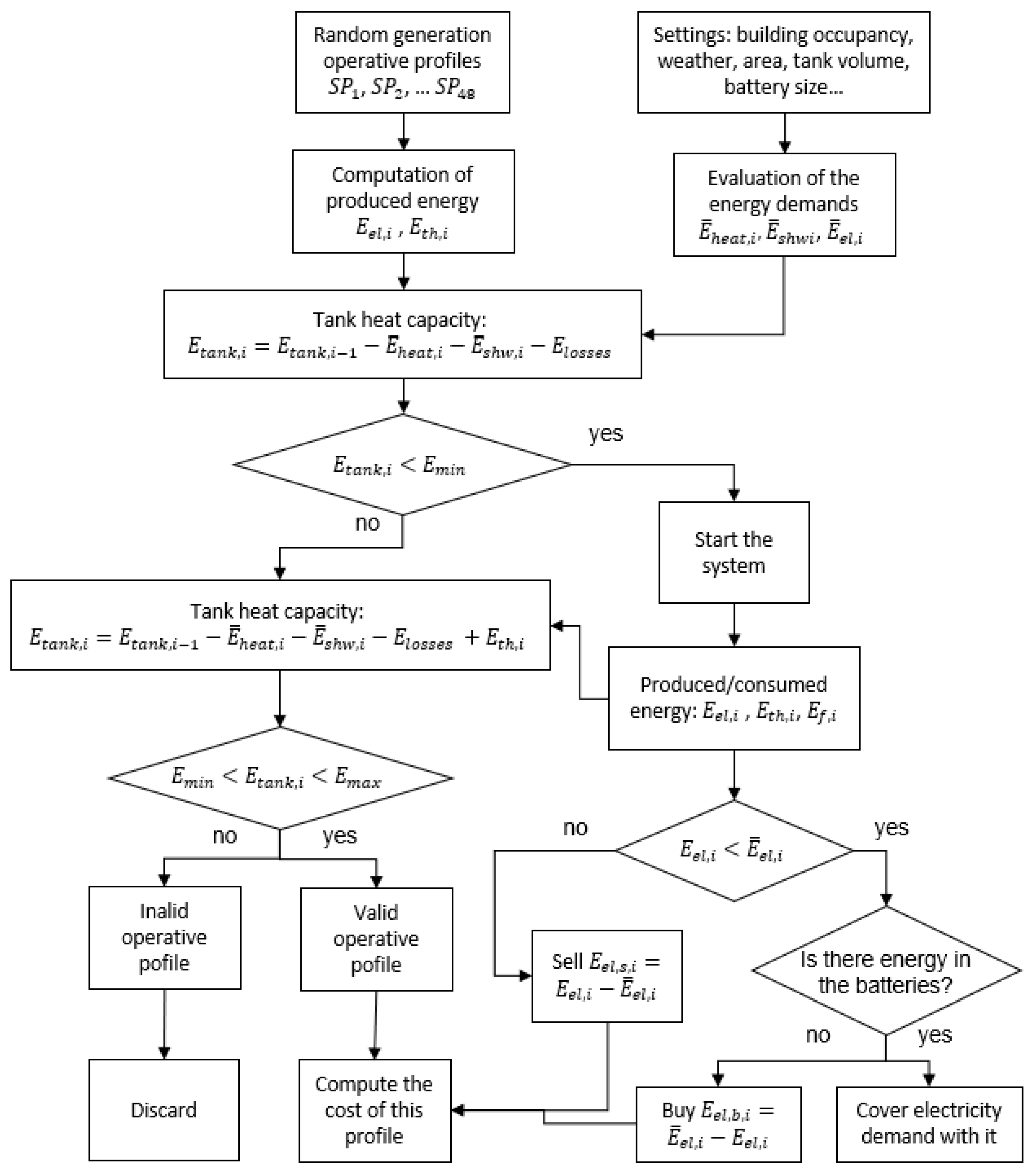
  • The system is running, and the demands are directly fulfilled with the energy produced;
  • The system is running, but there is partial or no demand: the water tank and the batteries are loaded. If the batteries are full, electricity can be fed back into the grid;
  • The system is not running, and the demands are fulfilled with the energy from the water tank and batteries. If the batteries are empty, electricity is provided from the grid;
  • The system is not running, and there is no demand: nothing happens, apart from heat losses removing heat from the water tank.
A compromise among the overall losses and fulfilling the demand and installation costs must be found. One of the novelties of this study is the sizing of thermal storage and batteries depending on the building size and the climate zone where the system is installed.
In order to fulfill the electrical and thermal power demands, MGTs can operate in a wide range of regimes, the so-called full-load and partial-load. The time sequence of the starts, stops, and operation points of the system over 24 h is called the operative profile. The scope of this paper is to determine the most economical operative profile of an MGT-based CHP system. This is done by means of an economic analysis via the optimization of the control strategy and the minimization of the total costs.
Daily and seasonable meteorological conditions significantly affect energy demand profiles [5]. The energy that the end-user needs in a typical day is a highly time-dependent profile, where the amplitude and frequency depend on different factors, such as how many people live/operate in the building, the weather, and the location. Therefore, if an MGT is supposed to work in such conditions, it should operate well in partial-load [6]. An optimal strategy has to be found between reduced electrical efficiency and power at partial-load in comparison to the start/stop and standby losses during intermittent operation. We sum up the major contributions and the novelties of this work as follows:
Major contributions:
  • The present work proves mathematically if operating an MGT-based CHP system at partial-load is economically more profitable than at full-load;
  • An algorithm to determine the most economical operative profile was developed and can be extended easily to other MGTs and countries as well;
  • This work provides clear guidelines for battery and water tank sizing depending on building size, occupancy, and climate zone;
  • This work constitutes the foundation of any lifetime prediction of MGT components, since it clearly defines the order and number or starts, stops, and loads, hence the working cycle.
Novelties:
  • Real-world energy demands (building occupancy, day of the week, season, weather, geographical area) are considered instead of constant values;
  • Batteries and thermal storage are examined together in the analysis (elsewhere often treated separately);
  • The possibility to feed the excess electricity back into the net is considered in the price function;
  • A finite price per day can be given for any operative profile, building size, day of the week, season, weather, or geographical area.

State-of-the-Art

In this paper, an MGT from the dutch company MTT, the Enertwin (3.2 kWel , 15.6 kWth ), is considered. Similar studies have been conducted, but either with the use of other power sources, such as solar, wind, and diesel sources [7], or with different MGTs, such as the Turbec T100 [8,9]. The work of [10] focused on the modeling approach of the MGT, but did not include the important role of thermal storage and batteries. A recent study [11] on hybrid photovoltaic–CHP systems involved the use of a much smaller CHP system (1 kWel, 2.4 kWth) and smaller thermal storage (300 L); instead, in the present analysis, a wide range of thermal storage and battery sizes is investigated. Much larger MGTs (65 kWel, 112 kWth) have been investigated as well in similar studies [12]. The role of the battery has also been analyzed in other works, as in [13,14] in connection with photovoltaic plants, but not with a single MGT.
Although MTT intends to enter markets in many regions of the world such as China, the U.S., and Canada, the commercialization focus from MTT is, as of 2019, mainly targeted at Europe [15]. For this reason, standardized load profiles for different types of households in Germany according to the norm VDI 4655 [16] are applied in this study. As a consequence, the numerical results (costs and operative profiles) are strictly valid for this country. However, considerations made for batteries and thermal storage have a broader validity and are of general interest. Moreover, the considerations made for the MTT Enertwin can be extended to other MGT-based CHP systems with a similar power range and contribute to the international community by providing clear control strategy guidelines. It is recommended that future studies perform similar economy-based analyses by considering energy demands and environmental factors from other countries; the flexibility of the algorithm presented here allows this with relatively small effort.
Data from experimental measurements conducted at the German Aerospace Center (Deutsches Zentrum fuer Luft- und Raumfahrt, DLR) are implemented in the algorithm, in addition to those of Maj and colleagues [17], who collected data on the same MGT and performed a preliminary study in this direction.
The paper is structured as follows: The experimental data and system properties are presented in the next section. The numerical algorithm, used to model the real system, will be presented in detail in the following section. The influence of the battery size, thermal storage tank size, climate zone, and other environmental factors is treated separately. The code is then used to provide general best practices for the control of the CHP system, in terms of starts, stops, and load points. Finally, results are discussed in the final section.

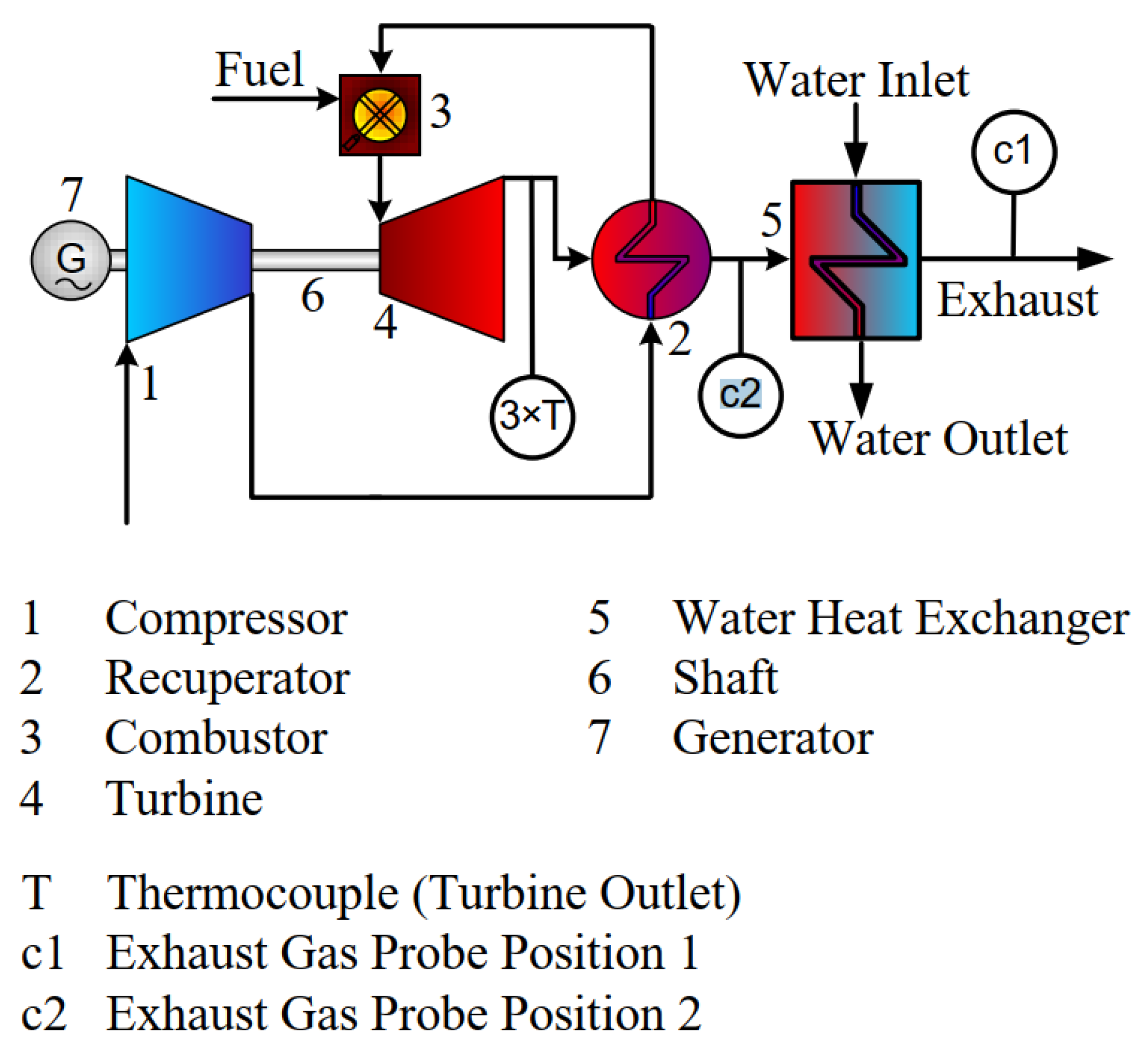
2. Experimental Data and Machine Characterization

An MGT MTT Enertwin was tested under various working conditions during experiments conducted at DLR, Stuttgart [18]. A schematic of the system and the instrumentation relevant for this paper is shown in Figure 1. At first, ambient air is compressed by the compressor (1) up to approximately 3 bars. Before entering the combustor (3), the air is pre-heated with hot exhaust gas in the recuperator (2). In the combustor, fuel (methane) is injected and oxidized and the hot exhaust gas is expanded through the turbine (4) and heats the compressed incoming fresh air in the recuperator (2). In the subsequent water heat exchanger (5), the thermal power (e.g., for use in heating systems) is coupled out. The compressor (1), turbine (4), and generator (7) are mounted on the same shaft (6). The oil pump and fuel pump are not shown in the scheme. The power needed to drive the compressor, P c , and the turbine power P t , can be calculated as:
P c = m ˙ a ( h 2 c h 1 c )
P t = ( m ˙ a + m ˙ f ) ( h 1 t h 2 t ) ,
where m ˙ a is the mass flow rate of inlet air, m ˙ f is the mass flow rate of fuel, and h 1 c , h 2 c , h 1 t , and h 2 t represent the enthalpy before and after the compression and the expansion (t = turbine), respectively. The MGT net shaft power, P M G T , is given by:
P M G T = P t P c P o i l P f , p u m p .
The power consumption of the oil pump and fuel pump is 75 W and 300 W, respectively. In this layout, the turbine shaft is connected to a high-speed electric generator, and a frequency inverter is needed to convert the high-frequency output of the electric generator to the grid frequency. The net electric power output is:
P e l = η g e n P M G T ,
where η g e n takes into account the losses of the electric generator and inverter. The energy balance at the water heat exchanger can be written as:
m ˙ a + m ˙ f m ˙ H 2 O = c p , H 2 O Δ T H 2 O h e x , 2 h e x , 1 ,
where m ˙ H 2 O , c p , H 2 O , and Δ T H 2 O are the water mass flow, specific heat, and temperature increase, respectively. h e x , 1 and h e x , 2 represent the enthalpy of exhaust gases before and after the heat exchanger. Finally, the thermal power produced by the CHP system is:
P t h = m ˙ H 2 O c p , H 2 O Δ T H 2 O .
At full-load, this system produces 3.2 kW electrical and 15.6 kW thermal power [19]. The built-in control software from MTT was modified and switched to manual mode (ProtoComm Manual Mode), so that the operators could test different maneuvers and operating points with more flexibility. The turbine outlet temperature is determined by the arithmetic average of three thermocouples (type K, tolerance class 2) with a measurement uncertainty of ±5.9 K. All other thermocouples were type N with tolerance class 1 and a resulting uncertainty of ±2.9 K. The MGT was controlled manually to a constant turbine outlet temperature of 1060 K by adjusting the fuel mass flow. The combustion chamber inlet temperature was in the range 725–734 C with a gas turbine pressure ratio of about 3. The fuel mass flow was measured with an F-211AV mass flow controller produced by Wagner-Bronkhorst with an accuracy of ± 0.5 % as a percentage of reading, plus ± 0.1 % full-scale. Fuel power is computed as:
P f = m ˙ f L H V ,
where m ˙ f is the fuel mass flow rate and L H V its Lower Heating Value. In this work, the MTT Enertwin works with methane with an L H V of 47.78 MJ/kg.
The operating point of the EnerTwin is expressed by a number called the Setting Point (SP). This value represents a percentage of the system load; full-load is characterized by SP = 100; partial-loads are in the interval 20 ≤ SP < 100; below SP = 20, the system cannot operate, and for SP = 0, the system is off. The system behavior at steady state will be presented in the next section. A maneuver is defined as the process of bringing the system from a steady state SP to another steady state SP; this characterization of the system will be treated in a following section. The maneuver starting from SP = 0 is called start; accordingly, in a stop maneuver, the final state is SP = 0. Operation in partial-load and the transient state is characterized by a smaller efficiency than at full-load, steady state. The electrical efficiency and total efficiency at partial-load are shown in Figure 2.

2.1. Steady State

For every SP, the MGT produces a certain amount of electrical power, requires a fuel mass flow to burn, and provides thermal power in terms of hot water mass flow. Table 1 shows thermal, fuel, and electrical power for different SPs. Please note that the value of P e l in the table is the net value of electrical power after deducting the power required to run the oil pump and fuel compressor.

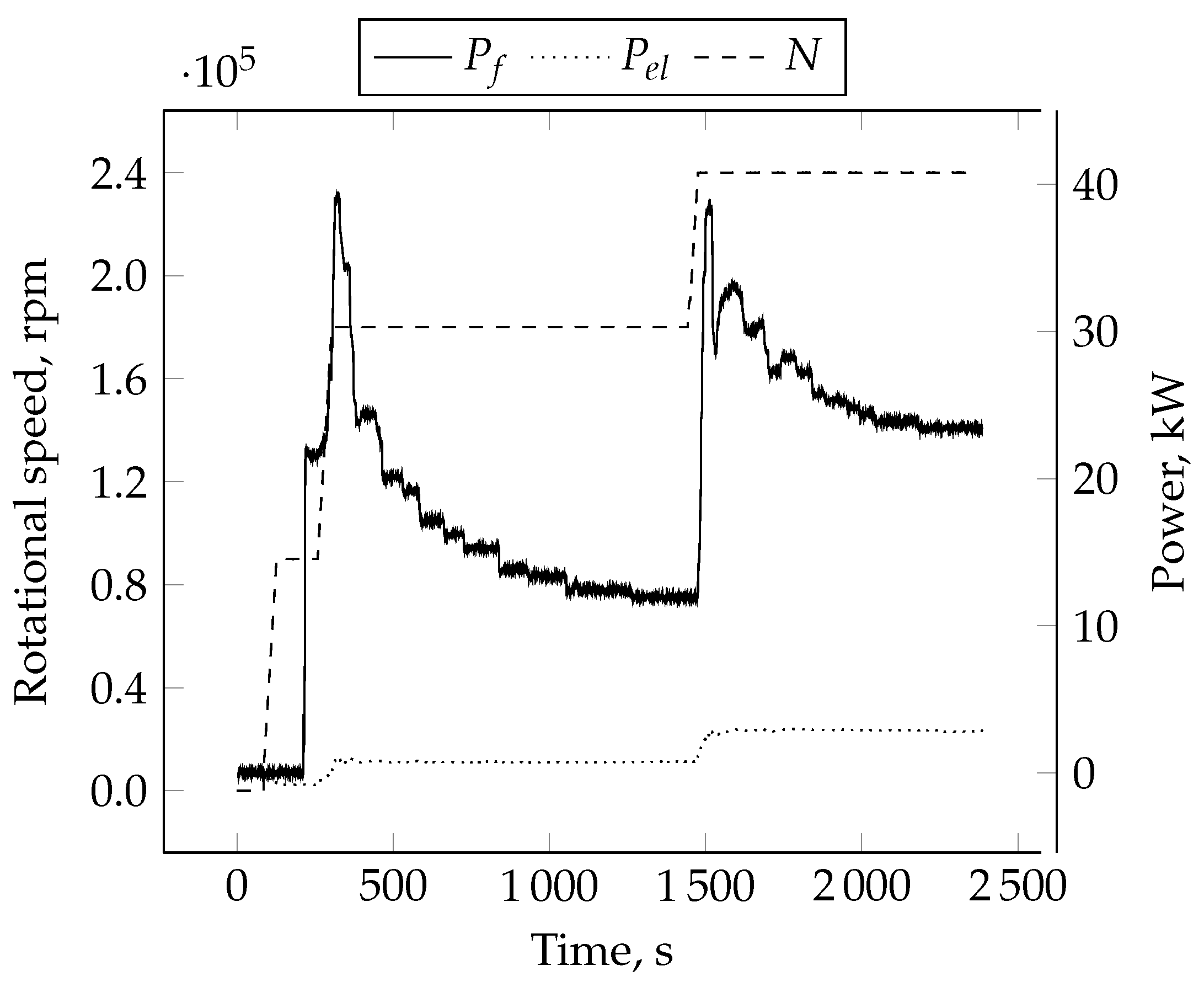
2.2. Transient State, Start, and Cool-Down

The measuring campaigns of MTT Enertwin conducted at DLR included not only steady state operations, but also accelerating and decelerating maneuvers. These are induced by increasing (or decreasing) the fuel mass flow to the combustion chamber; shaft rotational speed is monitored with a 2 Hz frequency. A maneuver is considered complete when both the rotational speed and fuel mass flow remain constant at the new SP. In Figure 3, a cold start maneuver is shown, in which the shaft’s rotational speed goes from 0 up to 240 krpm in a staged fashion.
During the first 4–5 min of the test, the system consumes electric power to drive the turbine up to N = 90 krpm, where ignition takes place. The system is then steadily accelerated up to 180 krpm, the so-called minimum load (SP = 20). After a first peak in the fuel mass flow rate, which is needed to start the cold system, fuel mass flow can be gradually reduced. A second peak allows the rotational speed to ramp-up to full-load, SP = 100, at 240 krpm. Just like in the work of Maj [17], the cold start maneuver is considered complete after about half an hour. However, the time to reach steady state depends on the initial temperature: the warmer the system, the faster it reaches the steady state. In Maj’s tests, 1700 s was the minimum time for the system to reach the steady state after a cold start; in warmer starts, the system reached the steady state earlier. The maneuver time was increased from 1700 s to 2000 s to ensure the steady state under every condition. The authors of the present work also believe that a cold start maneuver can be performed under every condition within 1800 s (exactly half an hour) by reducing the time of the staged fuel mass injection: the second fuel peak in Figure 3 could be anticipated at circa 400 s (the experiments conducted at DLR had multiple goals, and therefore, the maneuvers were performed as compromise between different requirements). Therefore, the present analysis assumes 1800 s as the minimum time to start the system.
Cool-down maneuvers were not investigated in detail during the measuring campaign, and the data from Maj were kept as a reference. Hence, 150 s was considered to be the time needed to reduce the speed of the engine to 0 rpm, for all loads. During cool-down, the heat exchanger is still warm and allows for further energy extraction; in particular, 0.455 kWh thermal and 0.011 kWh electric energy are produced during the 150 s of this maneuver.

3. Numerical Model

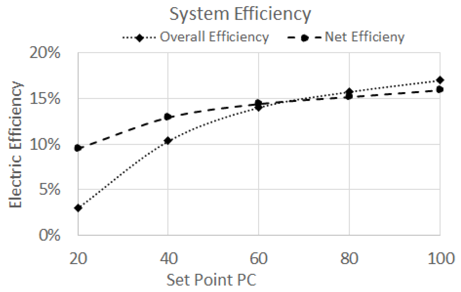
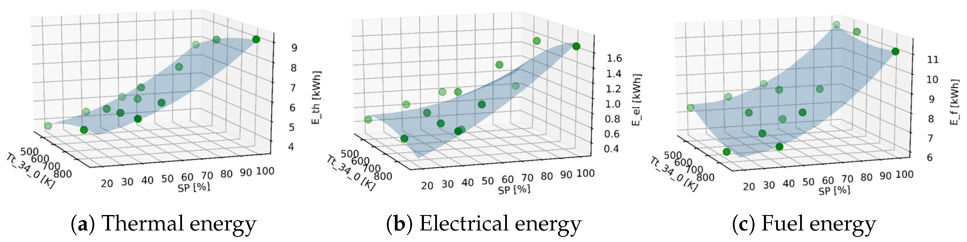
3.1. Performance Analysis

An operative profile is a set of 48 SP values in the range [0, 100] indicating the operating points of the system for each 30 min time step. The numerical model, implemented in the Python programming language for this analysis, generates n random operative profiles and evaluates if they fulfill the heat and electrical demand at every time step. If not, the solution is discarded and the next candidate is evaluated. If yes, the cost associated with this solution is computed by:
c o s t = i 48 E f · p f + E e l , b · p e l , b E e l , s · p e l , s i
where E f is the energy content of the fuel burned and p f the fuel price; E e l , b and E e l , s are the amounts of electrical energy bought and sold, and p e l , b , p e l , s their prices, respectively. The average electricity and methane prices between the years 2018 and 2019 in Germany were considered in this work [20]:
p f = 0.07   / kWh , p e l , b = 0.29   / kWh , p e l , s = 0.04   / kWh .
At the end of the analysis, the solution that minimizes the cost is selected and is considered to be the optimal operating profile of the MTT Enertwin.
Within one time step, the system requires as much fuel energy as E f kWh and produces the two forms of energies E t h and E e l , also in kWh. In the steady state:
E i = f ( SP ) = P i ( SP ) · Δ t i = t h , e l , f
where P i are shown in Table 1. In turn, during a start transient state, the system produces an amount of energy that is the integral during the 30 min ramp-up and is a function of the target SP and initial recuperator temperature:
E i = f ( T 34 , SP ) i = t h , e l , f
These values are modeled via 2D maps extrapolated from experimental data and shown in Figure 4. Finally, the electricity produced will rarely match exactly the electricity consumed by the user, E ¯ e l . Two scenarios are possible:
E e l = E ¯ e l E e l , b if E e l < E ¯ e l E ¯ e l + E e l , s if E e l > E ¯ e l .
meaning that if more energy is required than produced, the difference needs to be bought from the grid; if too much electricity is produced, the excess will be fed back into the grid. The energy demands from the user are real-life measured data according to norms and will be presented in Section 3.2.
The next meaningful question is how to determine weather or not a generated operative profile fulfills the demand. The key observation here is to guarantee that the heat capacity of the water tank must be always higher than the minimum threshold at every time step, otherwise the thermal demand cannot be fulfilled. This is expressed by:
E t a n k , m i n < E t a n k , i < E t a n k , m a x
c p V m i n T m i n < E t a n k , i < c p V m a x T m a x i .
More information concerning the water tank vessel volume and heat capacity are described in Section 3.3. When the system is off (hence, when SP = 0 at a certain time step), thermal capacity is drawn from the tank by the user, plus a small part is lost by convection. At a certain point, a minimum is reached: either a minimum threshold temperature is reached or too little water is present in the tank. At this moment, the system must be on in order to fulfill the demand. Operative profiles that do not guarantee this are not valid, hence discarded.

3.2. Energy Demand Profiles

The norm VDI 4655 [16] provides raw data about the typical electrical and thermal demand of small buildings in Germany. The daily energy consumption, expressed in kWh, is a value that depends on the building size, climate zone, week day, season, and weather. Following the norm, two types of buildings can be identified: Single-Family Houses (SFHs) and Multiple-Family Houses (MFHs). In this analysis, when referring to building size, this depends on the number of occupants in an SFH and on the number of families for an MFH. The other factors and their effects on energy demand will be explained in the following sections.
The daily overall energy demands are a fraction of the yearly energy consumption and are expressed by the following equations:
E ¯ h e a t , d = E ¯ h e a t , y · F h e a t ,
E ¯ e l , d = E ¯ e l , y 1 / 365 + N p p , f a m · F e l ,
E ¯ s h w , d = E ¯ s h w , y 1 / 365 + N p p , f a m · F s h w ,
where the suffixes h e a t , e l , and s h w indicate hot water for heating, electrical, and sanitary hot water, respectively; the letters d and y indicate the daily and yearly consumption, respectively, and the overbar indicates demand quantities, to avoid confusion with the produced quantities of the previous sections. N p p , f a m is an integer that indicates either the number of people per family or the number of families per building, depending on the building considered. The yearly values E ¯ e l , y and E ¯ s h w , y depend on building occupancy, while E ¯ h e a t , y depends on the effective house surface, expressed in square meters, as described in the norm DIN V 18599 [21]. Finally, the energy Factors F are penalty factors that depend on climate zone, week day, season, and weather. These factors are implemented in dictionary structures in the code, such that the right coefficient is used for every scenario.
In the norm, data on energy demand are sampled and made non-dimensional with a 2 s, 1 min, and 15 min frequency. Since the minimum time to start the system is 30 min, as explained in Section 2.2, in this analysis, pairs of data with a 15 min frequency are taken and summed, such that 48 points a day, 30 min each, are obtained (data sampled with a 2 s or 1 min frequency would bring the same result, when summed to form 30-min intervals).
The computation of the energy factors is reported in the next subsections. The energy demand of every 30 min time step i can be obtained by multiplying the non-dimensional demand shape, f i , by the daily energy demand:
E ¯ h e a t , i = f h e a t , i · E ¯ h e a t , d
E ¯ e l , i = f e l , i · E ¯ e l , d
E ¯ s h w , i = f s h w , i · E ¯ s h w , d

3.2.1. Climate Zones

The German Meteorological Service (DWD) monitors weather and meteorological conditions across the country and provides weather information for different purposes. In a study, DWD collected and sampled weather and environmental information for every hour for a year. According to the average external temperature, Germany can be divided into 15 different climate zones. For further information, the reader can refer to the norm DIN 4710 [22].

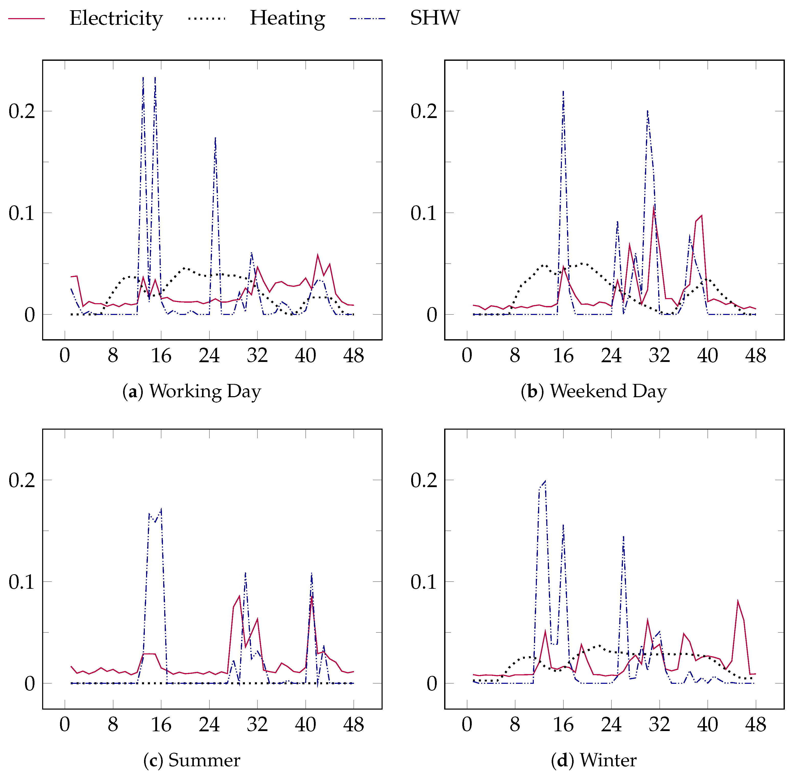
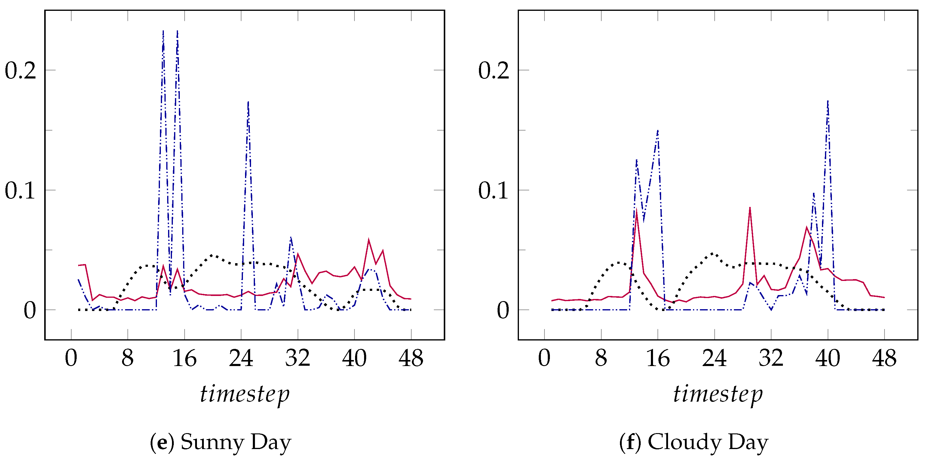
3.2.2. Day of the Week, Season, and Weather

The first external factor is the day of the week. The norm VDI 4655 distinguishes between Working day (W) and weekend day (S, for Sunday). In Figure 5a,b, the energy demand of these two typical days is compared, all the rest being equal. The most distinct difference is the time in which sanitary hot water is mostly needed, and at what intensity: mostly in the morning and at 12:00 during the week, whereas it is more smoothly distributed in the evening during the weekend.
The season can have a major impact on the energy demand of a house. Therefore, three different times of the year are defined: Summer (S), Winter (W) and intermediate seasons (U, from the German Uebergang, intermediate). The difference between summer and winter, all the rest being equal, is shown in Figure 5c,d as an example. It should be noted that in summer, no heating is needed. The demand of electricity in winter is more distributed during the day, whereas predominantly in the first afternoon and evening in summer.
The third environmental factor implemented in this analysis is the weather, distinguishing between sunny (H, from H e i t e r , clear) and cloudy days (B, from B e w o e l k t , cloudy). Since the weather in summer does not influence the average temperature significantly, only “neutral weather” (X) is considered for this season. Although the weather impact on the energy demand distribution is of minor importance, it was included for completeness. A comparison between a sunny day and a cloudy day can be seen in Figure 5e,f. In conclusion, the three above-mentioned external factors constitute ten different representative days in a year: UWH, UWB, USH, USB, SWX, SSX, WWH, WWB, WSH, WSB.

3.3. Convective Losses of the Thermal Storage Tank

The thermal storage tank is assumed to be of cylindrical form, and in particular, of that cylinder, proportions that minimize the external area. This is verified, regardless of the volume, when the cylinder height, H ¯ , equals its diameter, D. The tank is also assumed to be thermally insulated with a layer of polyurethane having a thermal conductivity of k = 0.03 W/mK at 80 C [23] and that the cylinder leans on the floor. Hence, convective thermal losses with the environment are computed accounting for the lateral and top surface only. Since heat losses depend on tank temperature and this, in turn, varies with time, heat loss coefficients must be computed at every time step.
For this simplified analysis, the tank surface temperature is assumed to be equal to the average temperature between the start and end of the time step (30 min); water stratification due to temperature gradients in the tank are not taken into account. For every time step, one Rayleigh number for natural convection is computed for the lateral surface and for the top of the cylinder:
R a 1 , 2 = g β ν α ( T s T ) L 1 , 2 3 L 1 = H ¯ lateral surface L 2 = D top surface
where g is the gravity acceleration, β is the air thermal expansion coefficient, ν is the kinematic viscosity, α is the thermal diffusivity, T and T s are the environment and the surface temperature, respectively, and L is a characteristic length, equal to D. The heat transfer coefficient can be computed as h 1 , 2 = k N u 1 , 2 / L 1 , 2 , where N u is the Nusselt number. Finally, the convective energy losses of the cylindrical water tank over the time step Δ t = 30 min are given by:
E l o s s , i = E l a t + E t o p = h 1 π D H ¯ + h 2 π ( D / 2 ) 2 ( T s T ) Δ t .
The energy stored in the tank at every time step i can be written as:
E t a n k , i = ( m H 2 O c p , H 2 O T H 2 O Δ t + E t h E ¯ h e a t E ¯ s h w E l o s s ) i
where T H 2 O is the water temperature, E t h is the thermal energy produced by the system and is given either by a steady-state operation (see Table 1) or by a maneuver, depending on SP and T 34 (Figure 4), E ¯ h e a t , i and E ¯ s h w , i are the thermal demands described by Equations (16) and (18). A scheme of the numerical solver is reported in Figure 6 for clarity.

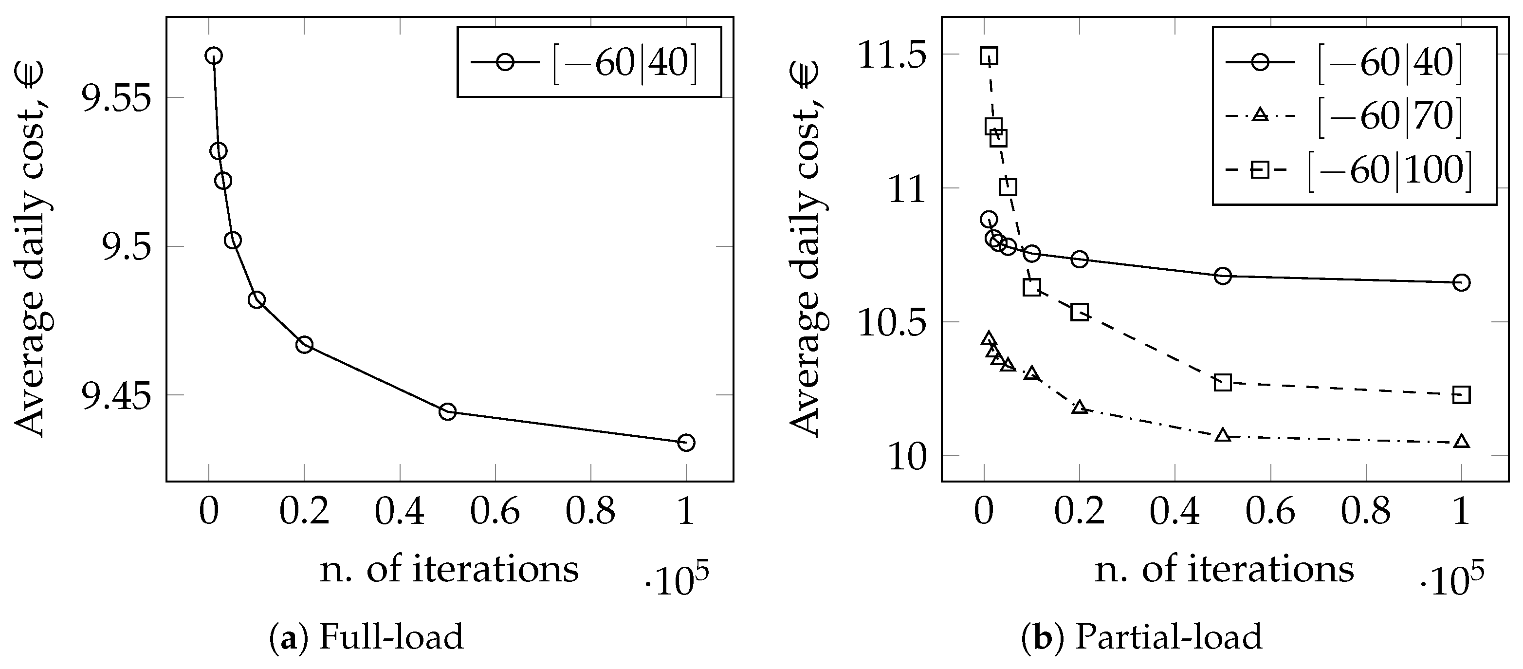
3.4. Optimization Process and Number of Iterations

In full-load mode, at each one of the 48 time steps, the turbine can be either on (SP = 100) or off (SP = 0). Thus, there are 2 48 possible operating profiles. The number is even higher when partial-load is considered, since 7 + 1 different operating points are possible (see Table 1). Exploring the complete space of possible solutions would require a huge amount of computational resources. Nevertheless, a large amount of solutions either do not fulfill the demand (too many SP = 0) or exceeded the amount of hot water that can be either consumed or saved in the tank. For this reason, “sampling” a smaller space of candidate solutions is sufficient to have an idea of the optimal operating profile. This procedure is explained in this section.
First of all, random solutions must be constrained within specific bounds. In order to have an equal probability of having the system operating or not, the SP values are searched within the bounds [−60, 100]. In fact, only SP values higher than or equal to 20 make it operate. Candidate solutions are pre-filtered such that, when SP < 20 are generated, they are automatically set to 0. However, it was noted that, by applying the SP pre-filtering in the interval [−60, 100], very expensive solutions were found. These solutions fulfill the energy demands, but do not minimize the costs. In fact, less expensive solutions could be found if the random search were influenced to look within more “low-power” bounds. A satisfactory interval was found to be [−60, 40] for the full-load mode: if SP < 20, SP is set to zero and the system is off, as usual. If 20 < SP < 40, however, SP is set to 100. In so doing, the solver is conditioned to look in a space where the system has a 80% probability to be off and 20% to be on. This conditioning also produced candidate solutions that fulfilled the demand, but with a final cost definitely lower.
For the partial-load, a similar approach was taken. Three different intervals were tested: [−60, 100], [−60, 70], and [−60, 40]. The first interval considers all the possible operating points; the second and the third consider only SP up to 70 and 40, respectively.
Figure 7 shows how the operative cost is influenced by the number of candidate solutions considered. Simulations were performed with n = 1k, 2k, 3 k, 5k, 10k, 50k, and 100k solutions. Results for full-load and partial-load operations are reported in Figure 7a,b, respectively. Both configurations show an asymptotic decreasing trend, since more candidates allow a higher chance to find a better solution. However, it can be seen that the curves flatten remarkably between 50k and 100k. Between these two points, there is a 0.11% variation (0.010 €) and 0.30% variation (0.031 €) for full-load and part-load mode, respectively. Hence, exploring a subset of n = 100k candidate solutions, instead of 2 48 or 8 48 , provides a satisfactory accuracy with much less computational cost. Future analyses could consider switching to a more efficient solver strategy instead of random search, for example a particle-swarm search, if similar accuracy were obtained with less computational time.
In Figure 7, it can be seen that the solutions generated within the [−60, 40] interval have small room for variation and provide very similar costs. On the other hand, when searching with few candidates within the [−60, 100] interval, expensive solutions (rich of SP = 80, 90, and 100) are found. By increasing n, less expensive solutions can be found. Finally, by allowing the solver to look for solutions within the [−60, 70] interval, more economical solutions are obtained. In any case, it can be seen that the full-load mode provides less expensive operating profiles compared to the partial-load mode. In the Results Section, a deeper comparison between these operative modes will be presented.

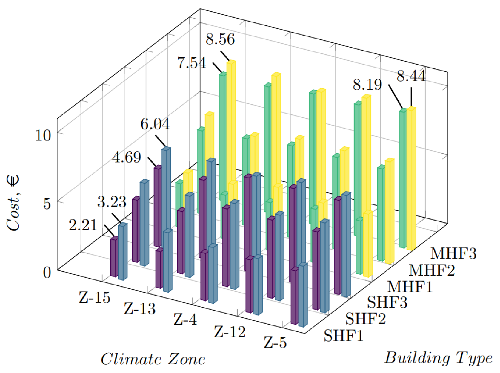
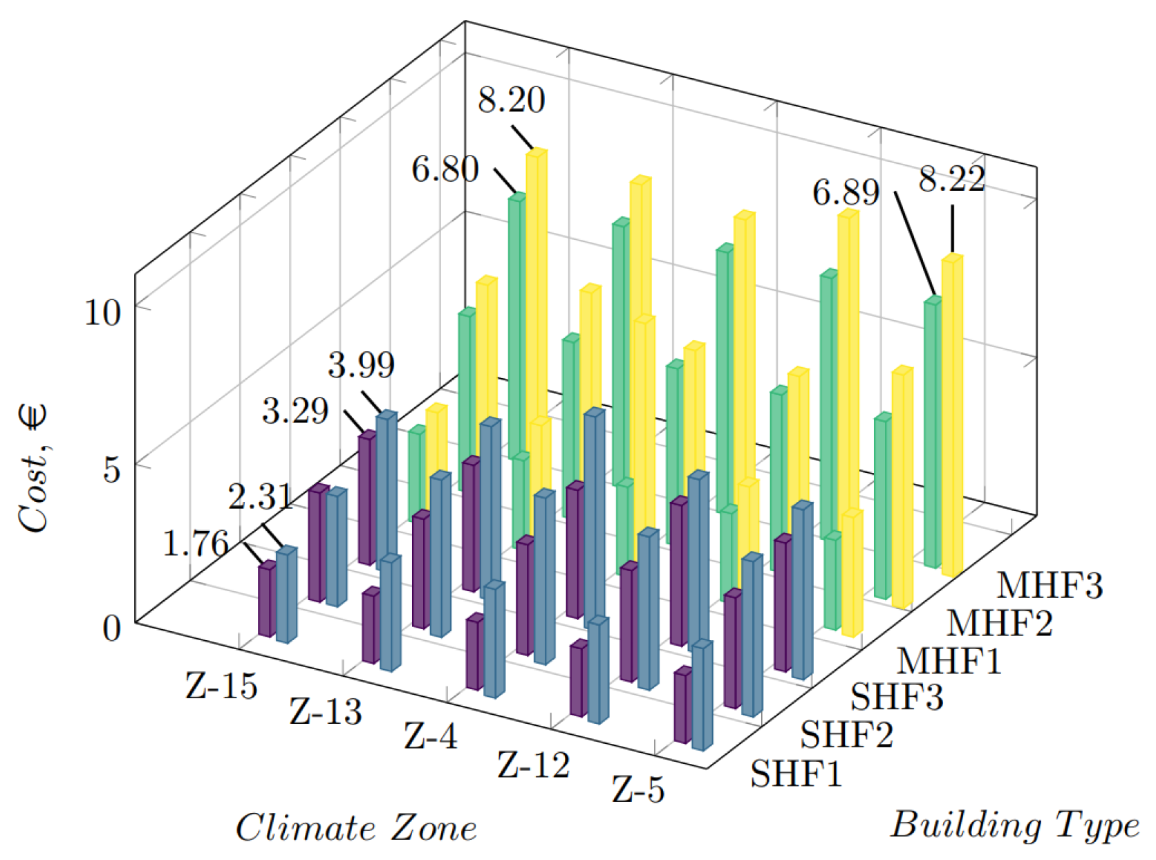
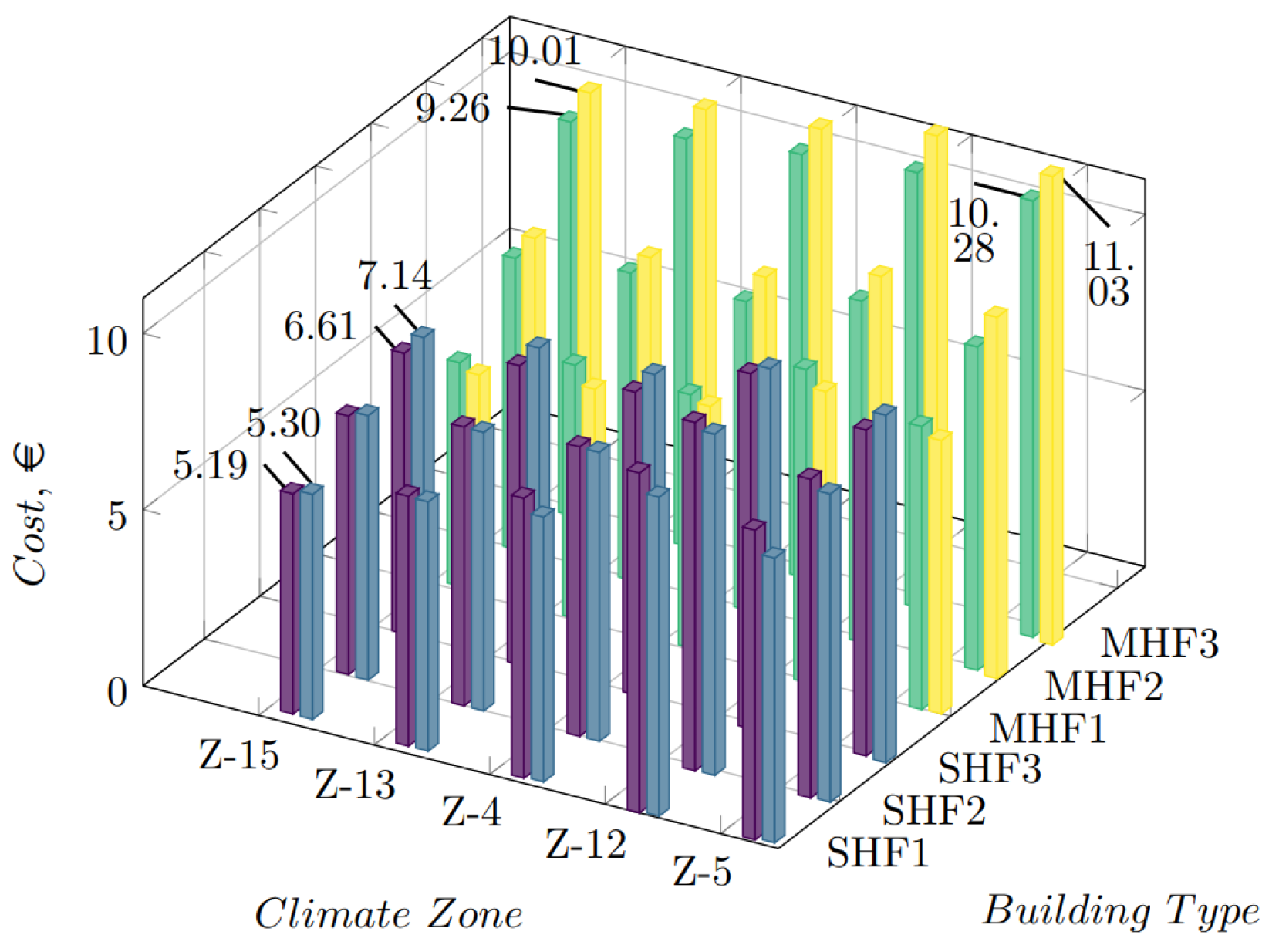
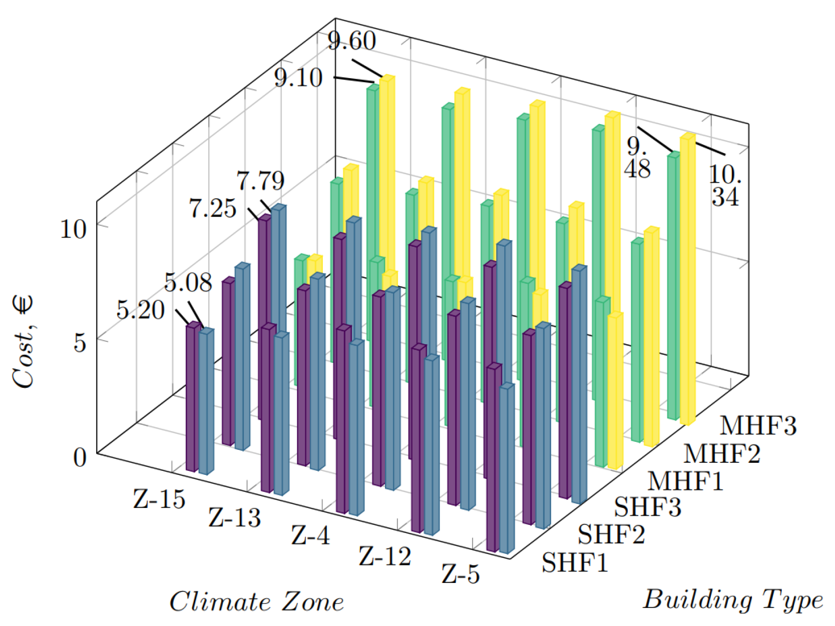
4. Results and Discussion

The mathematical model includes variables that are installation-dependent, such as battery and thermal storage size. A parametric study is conducted in Section 4.1 and Section 4.2 in order to define optimal values.

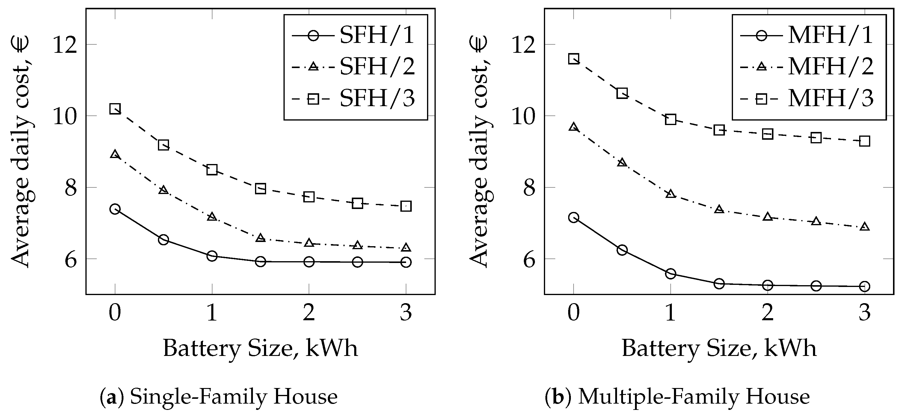
4.1. Influence of Battery Size

While the system is not running, the electricity demand must be fulfilled by relying either on the grid or on the batteries. In this section, the role of electricity storage is investigated, which has the potential to make the CHP-system more flexible and possibly grid-independent. In their analysis, Maj [17] did not account for batteries and assumed that the excess of electrical energy could be only injected into the grid. In the present analysis, the electric generator and the batteries are assumed to be ideal, meaning that no conversion losses are taken into account and that the energy stored in the batteries does not decrease due to the long storage time. These factors could quantitatively reduce the benefits shown in this section; however, they do not change the qualitative trends found here, which are the real focus of this study.
In Figure 8, the influence of battery size on the daily operative cost at full-load is shown. In Figure 8a, the operative cost for an SFH with one, two, and three occupants is plotted for different battery sizes. Similarly, an MFH with up to three families is taken into account in Figure 8b. It can be seen that even a small battery, up to 1 kWh, contributes to rapidly decreasing the costs. In fact, batteries allow a direct reduction of the electricity bought from the grid. The advantage of installing a battery strongly depends on the electricity prices. If buying 1 kWe from the grid costs more than selling it, which is usually the case, a battery could be convenient. In fact, it is more convenient to store the excess energy instead of selling it at a low price and buying eventually at a higher price when needed.
However, this advantage saturates when the battery size exceeds the needs of the building. It can be seen that small advantages are obtained for batteries larger than 1.5 kWh and that no further advantage is obtained over 2 kWh. In fact, beyond this size, the battery is so large that it is never completely charged. The installation cost, however, depends on size. For these reasons, a battery between 1.5 and 2 kWh is recommended for CHP systems that wish to be electrically independent and for reducing the operative costs.
The costs of a battery system vary with storage type and size. The average price of the main battery types in 2018 is reported in Table 2. It can be seen that the total project cost can vary between USD 469/kWh and USD 928/kWh [24]. The prices reported are expected to decrease by about 20–40% in 2025; also, the price per kWh generally decreases if larger systems are installed. Given their commercialization start in the early 1990s, Li-ion batteries are prevalent across a variety of industries, such as the electric automobile industry and the consumer electronics market, mainly in the MW range, due to their high specific energy, power, and performance. There have been successful deployments of Li-ion systems built for grid support up to several MW. Lead-acid and sodium–sulfur batteries are used across a wide variety of applications, but are not typically found in small, portable systems. Sodium metal halide batteries have primarily been introduced into the electrical storage market for EV usage; the battery sizes have a capacity range of between a few kWh and a few MWh and have a high level of scalability and flexibility. Due to their flexibility, sodium metal halide batteries are capable of being used across a large variety of applications, including EVs and public transportation, residential and commercial buildings, renewable generation smoothing, and others [25]. For their suitability and reliability in the small-grid kWh power range, sodium metal halide batteries were selected and implemented in this analysis.
A rough estimation from the data from Figure 8 shows that, by using a battery pack of 2 kWh, an average savings of EUR 2.10/day, hence EUR 760/year, can be obtained when compared to a scenario without batteries. Consequently, assuming installation costs of EUR 1800 for sodium metal halide batteries, the investment could be paid off in less than 3 years.
The status of battery charge during operation is depicted in Figure 9 for every time step. In this example, the most economical operative profile for the MGT operating in partial-load for a two-living-unit building is shown. The 2 kWh battery starts at 40% and the water tank at 75% of their respective maximum capacity. It can be seen that, when the system is not running, the electrical charge and the available hot water reduce due to the energy demand (not depicted here). When the system is activated (each column indicates the SP), the batteries are charged and hot water is produced. In can also be noted that, when the batteries are empty and the system is not running, electricity is taken from the grid (continuous line).

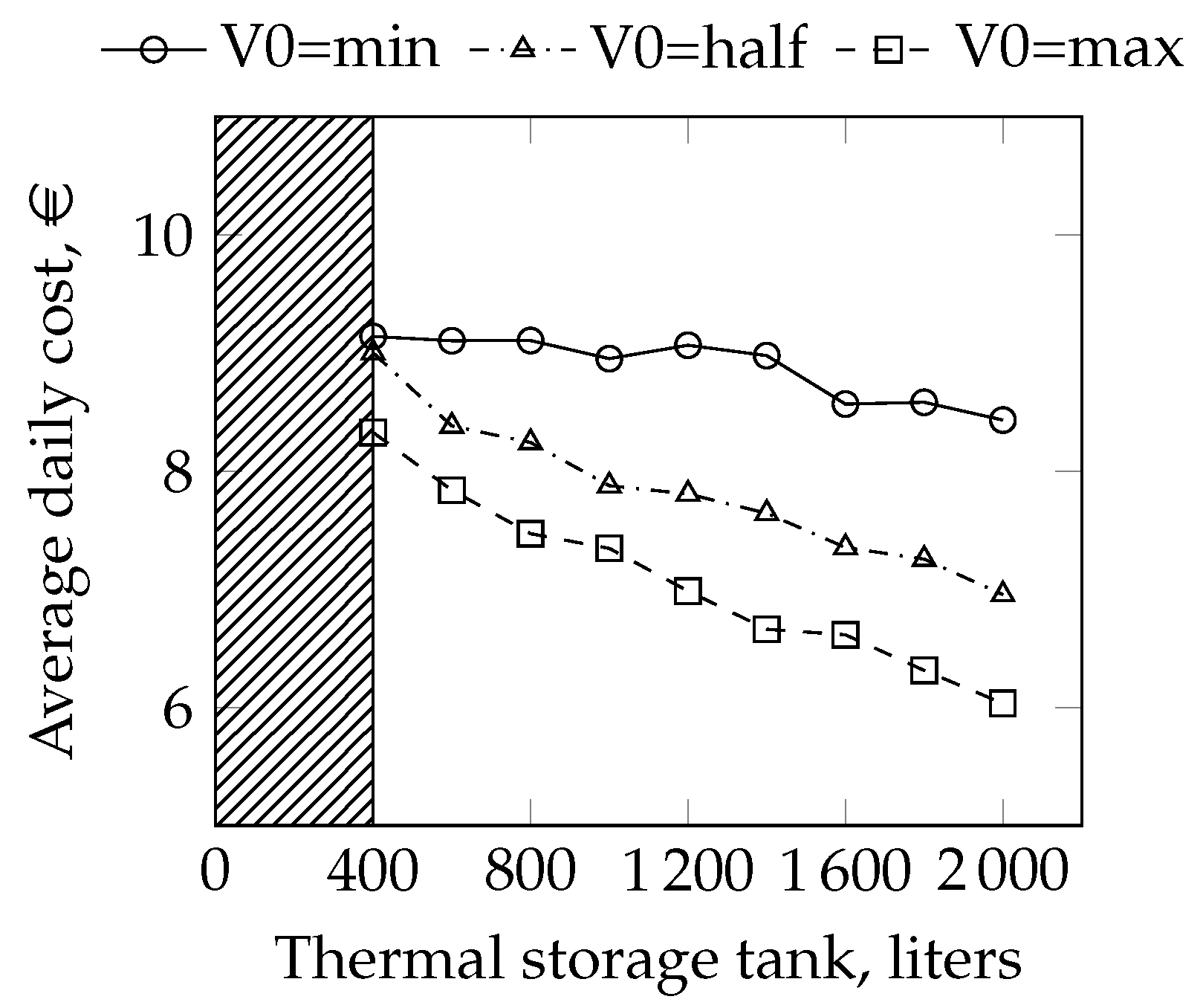
4.2. Influence of Thermal Storage Size

The thermal energy contained in the tank is subjected to convective losses, which are modeled in Section 3.3. Such losses depend, among other factors, on the exchange surface between the environment and the tank (the latter being already minimized by imposing H = D ). Hence, the bigger the tank, the larger the losses, all the rest being equal. However, a larger water tank allows more thermal heat storage, allowing the system, theoretically, to operate less often. The effect of these two counteracting phenomena is investigated in this section.
Figure 10 shows the influence of thermal storage size on operative cost for volumes up to 2000 L. V 0 is the relative amount of water at the beginning of the day, and simulations were conducted for V 0 = full, half, and empty tank. This parameter adds a further variable to the analysis of Maj [17], who only considered the case with a full initial tank. The results show a clear decreasing trend between operative cost and thermal storage size. This fact suggests that heat losses have a marginal role when compared to the gain of a larger tank. The importance of having hot water ready for use is further underlined by the three different configurations: when the day starts with a tank completely empty, more energy will be spent in the first hours to fill the tank and fulfill the demand at the same time. Finally, no valid operative solutions could be found for tanks smaller than 400 L with this setup.
It must be observed that, over long periods of time, the water tank will most probably start every day with different values of V0; moreover, in real applications, maximum and minimum thresholds both of water content and temperature are generally set. Nevertheless, this analysis shows that a minimum of 400 L is highly recommended and that larger water tanks are desirable in order to be progressively more thermally self-sufficient, depending on building size. Moreover, the German Federal Office of Economics and Export Control grants financing for those who desire installing CHP systems up to 20 kWel [26]. The MTT Enertwin, with its 3.2 kWel, fulfills the requirements and can benefit from a financing of up to EUR 3200, provided a thermal storage of minimum 936 L is installed.

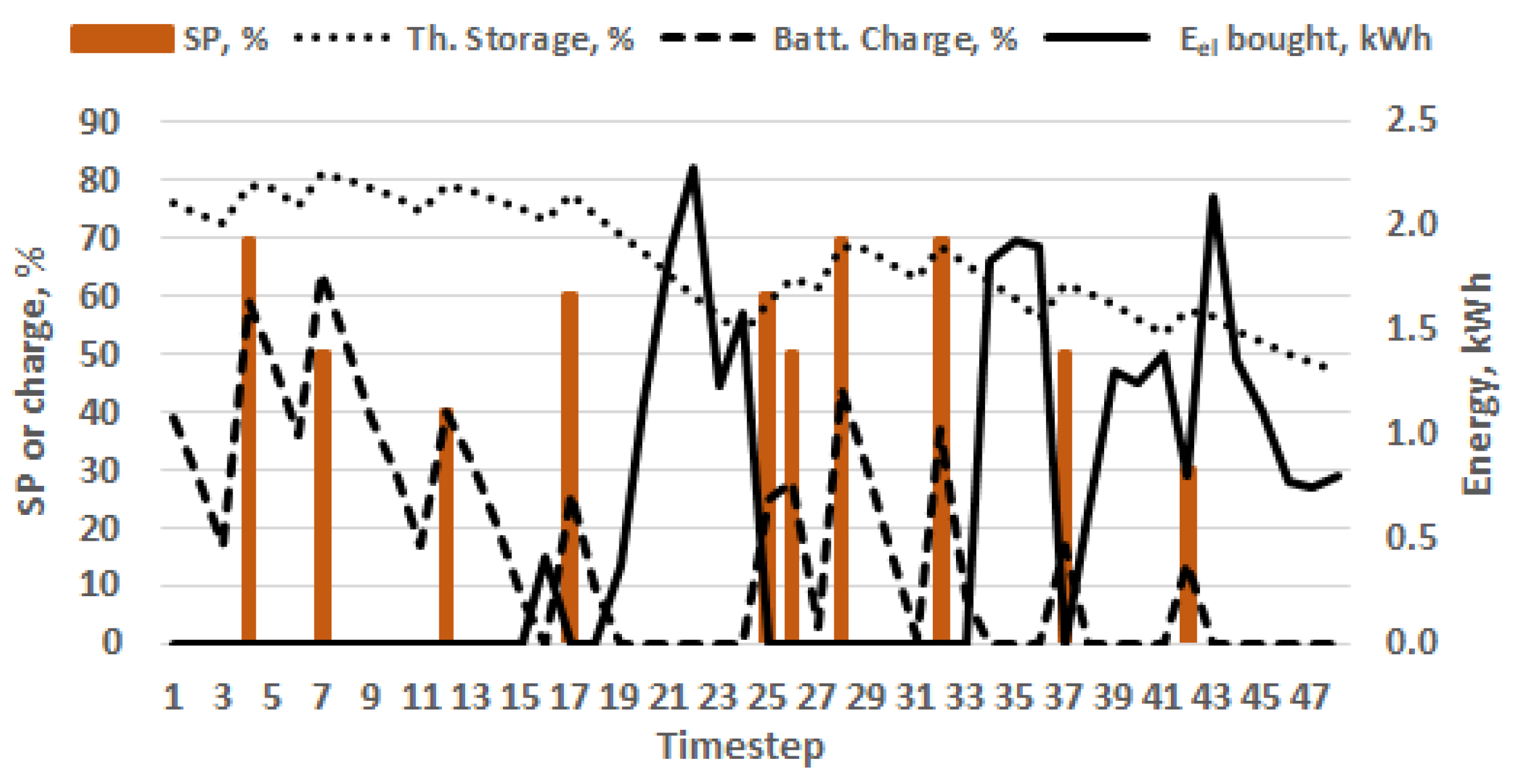
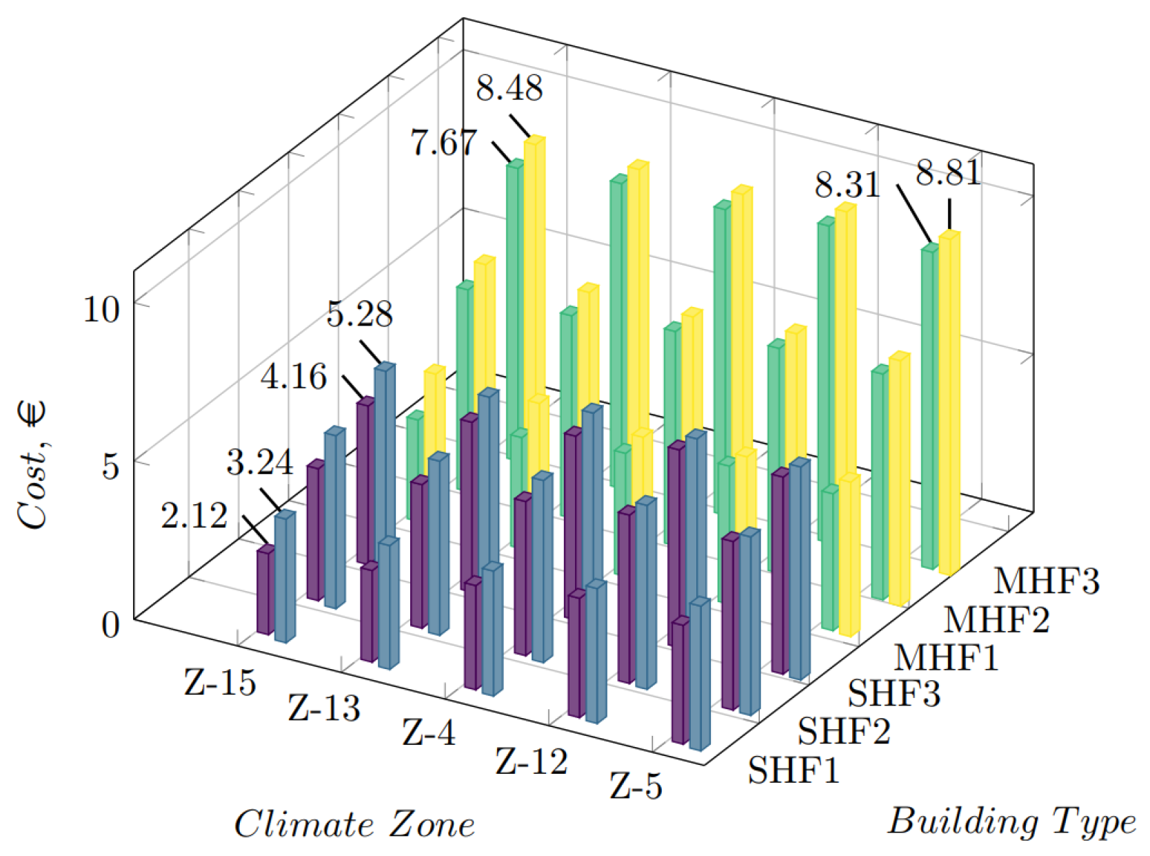
4.3. Determination of the Optimal Operative Profiles

The previous sections presented the influence of different algorithm parameters on the solution. In order to proceed further with the simulations, meaningful values should be chosen. For the following analysis, a battery of 2 kWh and a thermal storage of 1200 L were selected.
The simulations can investigate 15 climate zones, 10 typical days, and different building types and sizes. Moreover, for every scenario, two operating modes are investigated: full-load and partial-load. For the sake of brevity, only a part of these solutions is presented in this paper. A subset of five climate zones was selected: Z-15, Z-13, Z-4, Z-12, and Z-5. These zones are representative of the coldest and hottest climate zones in Germany and include a vast majority of its population.Furthermore, a subset of five typical days will be presented, covering all the seasons, days of the week, and weather: UWB, USB, SWX, WWB, WSB. Finally, the results of six building sizes are presented: SFH and MFH, with one, two, or three living units each.
In Figure 11, the results for the typical day UWB are presented. Similarly, the results for the other four typical days are reported in Figure 12, Figure 13, Figure 14 and Figure 15. The horizontal axes represent the climate zone and the building size. For every scenario, the darker column (purple and green) represents the operation at full-load, while the lighter column (blue and yellow) represents the operation at partial-load. The height of the column represents the daily operating cost of each scenario, in EUR, accounting for fuel consumed and electricity bought and sold from the grid (see Equation (8)). Some costs are shown with a label, in order to allow a comparison between climate zones, building size, and operating mode.
It can be seen that, for the intermediate seasons (Figure 11 and Figure 12), the operation at full-load is always more convenient of about 10–20%. Obviously, cost increases with building size and varies between 2.12 € (SFH1) and 8.81 € (MFH3). A small but consistent difference in cost is seen within climate zones: Z-15 generally requires the lowest costs, while Z-5 the highest. Furthermore, little difference can be seen between a working day and a weekend day, with no clear pattern: the operating cost difference for the same scenario between Figure 11 and Figure 12 lays within a few EUR cents.
In a typical summer day (Figure 13), the operating cost is significantly lower than in the intermediate seasons, because the thermal and electrical power demands are lower. Partial-load operation is, again, more expensive than the full-load operation of about 10–20%.
Finally, the results for typical winter days show, as expected, the highest operating costs. Zones 12 and 5 are characterized by the highest values, while Zone 5 by the lowest. It can be seen that, during winter working days (Figure 14), multiple climate zones for SFH1 and SFH2 and all the zones for MFH are characterized by a more convenient operation in partial-load. Similarly, during winter weekend days (Figure 15), all zones for SFH1 and some zones for MFH1 exhibit a more convenient partial-load operation.
This behavior indicates that partial-load operation has potential to be more convenient for small buildings (SFH1, SHF2, and MFH1) in the winter season, hence in those situations in which frequent, small consumption are needed. On the contrary, full-load operation remains the best operating mode for the vast majority of situations, in which larger amounts of thermal energy are requested rarely (in summer) or with a middle frequency from large multi-family buildings. In any case, full-load operation remains the safest choice for every scenario, since it guarantees the energy demands’ fulfillment, providing basically always the smallest costs.
As a final example, in Figure 16, the complete operative profile of two typical days in two climate zones is reported. Figure 16a,b show the most economical solution to fulfill the demand of a two-living-unit building, in an intermediate season, working, cloudy day in Climate Zone 15, in full-load and partial-load mode, respectively. A similar comparison is shown in Figure 16c,d for a winter, weekend, cloudy day in Climate Zone 13. Together with the SP profile, shown with columns, the status of the thermal storage is also plotted for every time step. In both scenarios, it can be seen that full-load mode fulfills the thermal and electrical demands, indicated with P t h and P e l , respectively, with a lower cost (10–15% less) and a lower number of starts/stops. This confirms the fact that it is generally not convenient to operate a CHP, MGT-based system in partial-load mode. Furthermore, a lower number of starts and stops might have the potential to spare some of the system components from alternating, thermo-mechanical fatigue. This aspect will be treated in a separate future work.

5. Conclusions

In this paper, the results of an economical optimization of the MGT MTT Enertwin were presented. The study aimed at determining whether an operation at partial-load could be economically more convenient than at full-load. Germany was selected as a case study, being Central Europe’s main market of this CHP. As constraints, the system had to fulfill two different heat demand profiles and comply with the electrical demand. The analysis spanned over 15 climate zones, investigated single-family and multi-family buildings, and included environmental and external elements such as weather, season, and day of the week.
This paper showed that an operation at full-load is, in the vast majority of cases, more convenient than at partial-load. The price difference is usually between 10% and 20%. This fact indicates that firing the system at full-load, but less frequently allows burning, in total, less fuel than firing more frequently at partial-load. The inefficiency of transient maneuvers and intermediate SP is the major cause for this result. The partial-load inefficiencies being a common characteristic of MGTs, this conclusion can be transferred to other MGT-based CHP systems as well.
A sensitivity study on the potential of batteries showed that their use is highly beneficial to reduce the operating costs. Depending on the building size, batteries between 1.5 and 3.0 kWh are recommended. The battery type can have a large impact on the installation costs and should be decided carefully. Installation costs are generally paid back within two or three years, depending on the electricity prices (sell/buy), hence on the agreements with the power provider.
A qualitative parametric study on the thermal storage size was also conducted, showing that larger water tanks allow for more flexibility and work like a thermal buffer. The advantages of having more water ready for use outweigh the higher thermal losses given by a larger tank, provided that this is properly thermally insulated. An upper limit for the tank size is not definable; however, a minimum of 1200 L is recommended in order to have enough operational flexibility and to possibly obtain, in some cases, incentives for the installation.
Finally, in the case of full-load mode, the system operating profile generally shows a lower number of starts and stops compared to partial-load. Since the transient loads are thought to be responsible for thermo-mechanical fatigue, a full-load operation could also be beneficial in terms of components’ life. Future studies from the same authors will investigate this topic in a future work.

Author Contributions

D.C.: conceptualization, methodology, software, formal analysis, data curation, writing—original draft. F.G.: writing—review and editing, supervision. P.K.: project administration. M.A.: funding acquisition. All authors have read and agreed to the published version of the manuscript.

Funding

This research received no external funding.

Data Availability Statement

Not applicable.

Acknowledgments

The authors would like to thank M. Maj and her colleagues from Lisbon University for setting the framework for this analysis and M. Herbst and H. Seliger-Ost (DLR Stuttgart) for the experimental data.

Conflicts of Interest

The authors declare no conflict of interest.

Abbreviations

The following abbreviations are used in this manuscript:
CHPCombined Heat and Power
DLRDeutsches Zentrum fuer Luft- und Raumfahrt
DWDGerman Meteorological Service
LHVLower Heating Value
MFHMultiple-Family House
MGTMicro Gas Turbine
SFHSingle-Family House
SHWSanitary Hot Water
SPSetting Point
SSXSummer, Weekend Day, Neutral Weather
SWXSummer, Working Day, Neutral Weather
TOTTurbine Outlet Temperature
USBIntermediate Season, Working Day, Cloudy
USHIntermediate Season, Working Day, Sunny
UWBIntermediate Season, Weekend Day, Cloudy
UWHIntermediate Season, Weekend Day, Sunny
WSBWinter, Weekend Day, Cloudy
WSHWinter, Weekend Day, Sunny
WWBWinter, Working Day, Cloudy
WWHWinter, Working Day, Sunny

References

  1. Beith, R. Small and Micro Combined Heat and Power (CHP) Systems; Woodhead Publishing Series in Energy; Woodhead Publishing Limited: Cambridge, UK, 2011. [Google Scholar]
  2. Ma, Z.; Knotzer, A.; Billanes, J.D.; Jørgensen, B.N. A literature review of energy flexibility in district heating with a survey of the stakeholders’ participation. Renew. Sustain. Energy Rev. 2020, 123, 109750. [Google Scholar] [CrossRef]
  3. González-Pino, I.; Pérez-Iribarren, E.; Campos-Celador, A.; Terés-Zubiaga, J. Analysis of the integration of micro-cogeneration units in space heating and domestic hot water plants. Energy 2020, 200, 117584. [Google Scholar] [CrossRef]
  4. Sayegh, M.; Danielewicz, J.; Nannou, T.; Miniewicz, M.; Jadwiszczak, P.; Piekarska, K.; Jouhara, H. Trends of European research and development in district heating technologies. Renew. Sustain. Energy Rev. 2017, 68, 1183–1192. [Google Scholar] [CrossRef] [Green Version]
  5. Reinders, A.; Verlinden, P.; Van Sark, W.; Freundlich, A. Photovoltaic Solar Energy: From Fundamentals to Applications; John Wiley & Sons: Hoboken, NJ, USA, 2017. [Google Scholar]
  6. Ebrahimi, M.; Keshavarz, A. 3-CCHP Evaluation Criteria. In Combined Cooling, Heating and Power; Ebrahimi, M., Keshavarz, A., Eds.; Elsevier: Boston, MA, USA, 2015; pp. 93–102. [Google Scholar] [CrossRef]
  7. Wang, X.; Palazoglu, A.; El-Farra, N.H. Operational optimization and demand response of hybrid renewable energy systems. Appl. Energy 2015, 143, 324–335. [Google Scholar] [CrossRef]
  8. Paepe, W.D.; Abraham, S.; Tsirikoglou, P.; Contino, F.; Parente, A.; Ghorbaniasl, G. Operational Optimization of a Typical micro Gas Turbine. Energy Procedia 2017, 142, 1653–1660. [Google Scholar] [CrossRef]
  9. Camporeale, S.M.; Fortunato, B.; Torresi, M.; Turi, F.; Pantaleo, A.M.; Pellerano, A. Part Load Performance and Operating Strategies of a Natural Gas—Biomass Dual Fueled Microturbine for Combined Heat and Power Generation. J. Eng. Gas Turbines Power 2015, 137, 121401. [Google Scholar] [CrossRef]
  10. Gimelli, A.; Sannino, R. A Micro Gas Turbine one-dimensional model: Approach description, calibration with a vector optimization methodology and validation. Appl. Therm. Eng. 2021, 188, 116644. [Google Scholar] [CrossRef]
  11. Kneiske, T.M.; Braun, M. Flexibility potentials of a combined use of heat storages and batteries in PV-CHP hybrid systems. Energy Procedia 2017, 135, 482–495. [Google Scholar] [CrossRef]
  12. Thu, K.; Saha, B.B.; Chua, K.J.; Bui, T.D. Thermodynamic analysis on the part-load performance of a microturbine system for micro/mini-CHP applications. Appl. Energy 2016, 178, 600–608. [Google Scholar] [CrossRef]
  13. Zhang, H.; Cai, J.; Fang, K.; Zhao, F.; Sutherland, J.W. Operational optimization of a grid-connected factory with onsite photovoltaic and battery storage systems. Appl. Energy 2017, 205, 1538–1547. [Google Scholar] [CrossRef]
  14. Gercek, C.; Reinders, A. Smart Appliances for Efficient Integration of Solar Energy: A Dutch Case Study of a Residential Smart Grid Pilot. Appl. Sci. 2019, 9, 581. [Google Scholar] [CrossRef] [Green Version]
  15. Ahout, W.; Hamilton, L. A Different Approach to Micro CHP, Final Report; Europe Commission H2020 Framework Programme. 2019, Volume 701006. Available online: https://cordis.europa.eu/project/id/701006/results/de (accessed on 11 May 2022).
  16. VDI 4655; Reference Load Profiles of Residential Buildings for Power, Heat and Domestic Hot Water as Well as Reference Generation Profiles for Photovoltaic Plants. Deutsche Institut für Normung e. V. (DIN): Berlin, Germany, 2019.
  17. Maj, M. Optimized Operation of the MTT EnerTwin in Non-Continuous or Part Load Operation. Master’s Thesis, Instituto Superior Técnico Lisbon, Lisbon, Portugal, 2017. [Google Scholar]
  18. Seliger-Ost, H.; Kutne, P.; Zanger, J.; Aigner, M. Experimental Investigation of the Impact of Biogas on a 3 kW Micro Gas Turbine FLOX®-based Combustor. In Turbo Expo: Power for Land, Sea, and Air; Volume 4B: Combustion, Fuels, and Emissions; American Society of Mechanical Engineers: New York, NY, USA, 2020. [Google Scholar] [CrossRef]
  19. Visser, W.P.J.; Shakariyants, S.; de Later, M.T.L.; Ayed, A.H.; Kusterer, K. Performance Optimization of a 3kW Microturbine for CHP Applications. In Manufacturing Materials and Metallurgy—Marine Microturbines and Small Turbomachinery—Supercritical CO2 Power Cycles; ASME International: New York, NY, USA, 2012; Volume 5, pp. 619–628. [Google Scholar] [CrossRef]
  20. Federal Network Agency. Annual Report for Electricity Prices, Federal Network Agency (Bundesnetzagentur). 2020. Available online: https://www.bundesnetzagentur.de/EN/General/Bundesnetzagentur/Publications/publications_node.html (accessed on 11 May 2022).
  21. DIN 18599; Energy Efficiency of Buildings—Calculation of the Net, Final and Primary Energy Demand for Heating, Cooling, Ventilation, Domestic Hot Water and Lighting—Part 1: General Balancing Procedures, Terms and Definitions, Zoning and Evaluation Of Energy Sources. Deutsche Institut für Normung e. V. (DIN): Berlin, Germany, 2018.
  22. DIN 4710; Meteorological Data for Technical Building Services Purposes—Degree Days. Deutsche Institut für Normung e. V. (DIN): Berlin, Germany, 2007.
  23. Pau, D.S.W.; Fleischmann, C.M.; Spearpoint, M.J.; Li, K.Y. Thermophysical properties of polyurethane foams and their melts. Fire Mater. 2013, 38, 433–450. [Google Scholar] [CrossRef]
  24. Mongird, K.; Viswanathan, V.V.; Balducci, P.J.; Alam, M.J.E.; Fotedar, V.; Koritarov, V.S.; Hadjerioua, B. Energy Storage Technology and Cost Characterization Report; US Department of Energies, Pacific Northwest National Laboratory (PNNL): Richland, WA, USA, 2019. [CrossRef]
  25. EASE (European Association for Energy Storage). Energy Storage Technologies; EASE (European Association for Energy Storage): Brussels, Belgium, 2016; Available online: https://ease-storage.eu/energy-storage/technologies/ (accessed on 11 May 2022).
  26. Financing for Mini-CHP Systems up to 20 kWel; Federal Office of Economics and Export Control (Bundesamt für Wirtschaft und Ausfuhrkontrolle): Eschborn, Germany, 2020; Available online: https://www.bafa.de/DE/Energie/Energieeffizienz/Kraft_Waerme_Kopplung/Mini_KWK/mini_kwk_node.html (accessed on 11 May 2022).
Figure 1. The micro gas turbine MTT Enertwin in its combined heat and power configuration.
Applsci 12 06069 g001
Figure 2. Global and net efficiency of the MTT Enertwin as measured by [17]. Adapted from [17]. Copyright 2017, Instituto Superior Técnico Lisbon.
Applsci 12 06069 g002
Figure 3. Cold start maneuver up to full-load, steady state. T r e c = 450 K. P e l = electrical power, P f = fuel power, and N = rotational speed.
Applsci 12 06069 g003
Figure 4. The 2D interpolating maps allowing obtaining the energy produced during transient maneuvers. Starting from a recuperator temperature (left horizontal axis) and given the final SP (right horizontal axis), the thermal, electrical, and fuel energy can be read on the vertical axis, respectively.
Applsci 12 06069 g004
Figure 5. Non-dimensional energy demand profiles. Effect of weekday ((a) vs. (b)), season ((c) vs. (d)), and weather ((e) vs. (f)) on time and intensity distributions for a single-family building.
Applsci 12 06069 g005aApplsci 12 06069 g005b
Figure 6. Flowchart of the developed optimization algorithm for the MGT-CHP system. Each randomly generated operative profile is tested. The energy demands are assigned as the input, based on environmental parameters and building occupancy and size. Battery and thermal storage sizes are assigned by the user, and their charge is updated for every time step. If the system fulfills the demand, the operative profile cost is computed; if not, it is discarded and the next one is analyzed.
Applsci 12 06069 g006
Figure 7. Daily cost for different iterations. Climate Zone 5, multiple family house, 3 families, setting WSB, battery 2 kWh, tank volume 800 L.
Applsci 12 06069 g007
Figure 8. Influence of battery size on daily cost, for different house occupancies for SFH (a) and number of families per MFH (b). Climate Zone 5, setting WSB, tank 800 L, full-load.
Applsci 12 06069 g008
Figure 9. Battery charge/discharge status at every time interval of the operation period. Climate Zone 13, typical day WSB, battery 2 kWh, thermal storage 1200 L, operation partial-load.
Applsci 12 06069 g009
Figure 10. Influence of water tank size on daily cost, for different initial water levels. Climate Zone 5, typical day WSB, battery 2 kWh, operation full-load.
Applsci 12 06069 g010
Figure 11. Cost comparison between full-load (left column, purple, and green) and partial-load operation (right column, blue, and yellow) for different climate zones and building types, for a UWB typical day (intermediate season, working day, cloudy).
Applsci 12 06069 g011
Figure 12. Cost comparison between full-load (left column, purple and green) and partial-load operation (right column, blue and yellow) for different climate zones and building types, for a USB typical day (intermediate season, weekend day, cloudy).
Applsci 12 06069 g012
Figure 13. Cost comparison between full-load (left column, purple and green) and partial-load operation (right column, blue and yellow) for different climate zones and building types, for an SWX typical day (summer, working day, neutral weather).
Applsci 12 06069 g013
Figure 14. Cost comparison between full-load (left column, purple and green) and partial-load operation (right column, blue and yellow) for different climate zones and building types, for a WWB typical day (winter, working day, cloudy).
Applsci 12 06069 g014
Figure 15. Cost comparison between full-load (left column, purple and green) and partial-load operation (right column, blue and yellow) for different climate zones and building types, for a WSB typical day (winter, weekend day, cloudy).
Applsci 12 06069 g015
Figure 16. Comparison of the optimal operating profile for two example scenarios: climate zone 15, typical day UWB (a,b), and climate zone 13, typical day WSB (c,d). On the left, the full-load mode, on the right, the partial-load mode, for a 2-living-unit building.
Applsci 12 06069 g016
Table 1. Steady state properties at various setting points. N = rotational speed, P t h = thermal power, P e l = electrical power, and P f = fuel power.
SPN (krpm) P th (kW) P el (kW) P f (kW)
PC201807.600.7310.56
PC401908.401.0211.96
PC6020010.001.3413.44
PC7021011.301.6915.46
PC8022012.502.0417.54
PC9023014.202.3919.77
PC10024015.602.7022.17
Table 2. Summary of battery types and costs for CHP applications in 2018 according to [24]. Data from [24]. Copyright 2019, U.S. Department of Energy (DOE) Pacific Northwest National Lab. (PNNL-28866).
ParameterSodium–SulfurLi-IonLead AcidSodium Metal
Capital Cost-Energy Capacity (USD/kWh)661271260700
Power Conversion System (PCS) (USD/kW)350288350350
Balance of Plant (BOP) (USD/kW)100100100100
Construction and Commissioning (USD/kWh)133101176115
Total Project Cost (USD/kWh)907469549928
Publisher’s Note: MDPI stays neutral with regard to jurisdictional claims in published maps and institutional affiliations.

