
Aerodynamic-Aeroacoustic Optimization of a Baseline Wing and Flap Configuration
by
 ,
,
Shengjun Ju
1,2, 
Zhenxu Sun
1,2,*,
Dilong Guo
1,2,
Guowei Yang
1,2,
Yeteng Wang
1,2 and
Chang Yan
1,2 1
Key Laboratory for Mechanics in Fluid Solid Coupling Systems, Institute of Mechanics, Chinese Academy of Sciences, Beijing 100190, China
2
College of Engineering Sciences, University of Chinese Academy of Sciences, Beijing 100049, China
*
Author to whom correspondence should be addressed.
Appl. Sci. 2022, 12(3), 1063; https://0-doi-org.brum.beds.ac.uk/10.3390/app12031063
Submission received: 29 November 2021
/
Revised: 7 January 2022
/
Accepted: 11 January 2022
/
Published: 20 January 2022
(This article belongs to the Special Issue Structural Vibration: Analysis, Control, Experiment, and Applications II)
Abstract
:Optimization design was widely used in the high-lift device design process, and the aeroacoustic reduction characteristic is an important objective of the optimization. The aerodynamic and aeroacoustic study on the baseline wing and flap configuration was performed numerically. In the current study, the three-dimensional Large Eddy Simulation (LES) equations coupled with dynamic Smagorinsky subgrid model and Ffowcs–William and Hawkings (FW–H) equation are employed to simulate the flow fields and carry out acoustic analogy. The numerical results show reasonable agreement with the experimental data. Further, the particle swarm optimization algorithm coupled with the Kriging surrogate model was employed to determine optimum location of the flap deposition. The Latin hypercube method is used for the generation of initial samples for optimization. In addition, the relationship between the design variables and the objective functions are obtained using the optimization sample points. The optimized maximum overall sound pressure level (OASPL) of far-field noise decreases by 3.99 dB with a loss of lift-drag ratio (L/D) of less than 1%. Meanwhile, the optimized performances are in good and reasonable agreement with the numerical predictions. The findings provide suggestions for the low-noise and high-lift configuration design and application in high-lift devices.
1. Introduction
With the rapid development of civil aviation, aeroacoustic problems were of wide concern among aviation manufacturing enterprises and researchers the world over. Strict noise airworthiness regulations are formulated by the International Civil Aviation Organization (ICAO) to limit the noise of civil aircraft. The research projects to reduce the noise level of civil aircraft were developed by the European Advisory Committee on Aeronautical Research (ACARE) [1] and the National Aeronautics and Space Administration (NASA) [2].
During takeoff and landing of civil aircraft, the flap lifting device is one of the main components that produce noise [3]. In the noise generated by flap lifting device, the side edge vortex shedding of the flap is the main noise source [4].
The research on the flap side edge noise source can be traced back to 1979, when Fink [5] and Schlinker [6] found that the flap side edge was an important aircraft noise source. Meecham et al. [7] confirmed the existence of severe surface pressure fluctuation in the flap tip region and demonstrated that the formation of pressure fluctuation is directly related to the coherent structures in the shear layer. Khorrami et al. [8] analyzed and showed that the unstable wave in the lateral shear layer is the main cause of noise by using the instability theory.
With the continuous progress of measurement technology, the understanding of flap side edge noise was deepened. Streett [9] and Radezrsky [10] et al. respectively carried out several experiments on the side flow field of trailing edge flap. The flow field at different deflection angles were measured experimentally. They found that there is a vortex pair structure at the side edge of the flap. The result showed that the vortex breaking mechanism can induce noise under the condition of a large deflection angle. Moreover, a series of aeroacoustic experiments on the far-field noise of flap was carried out by Rackl et al. [11]. They found that reasonable geometric position and structural deformation can reduce the noise radiation of slat to a certain extent and maintain high aerodynamic performance.
In recent years, the Computational Fluid Dynamics (CFD) and Computational Aero-Acoustics (CAA) were widely employed in the flow features and noise of wing-flap configuration [12]. The numerical investigation of unsteady flow field around high-lift device was presented by Satti [13] using the Lattice Boltzmann method (LBM). The pressure fluctuation and aeroacoustics analysis of the high-lift airfoil was obtained. The numerical results showed that predictions of noise sources and their relative strengths were in good and reasonable agreement with the experimental data from microphone array measurements.
The interference between the shear layer unstable wave and the upper and lower walls of the flap by using the CFD/CAA hybrid method was carried out by Dong et al. [14] and Rakhshanil et al. [15] also performed a series of unsteady turbulent fluctuations in the acoustic source surface of high-lift device. The transient flow field was obtained by solving the Unsteady Reynolds Averaged Navier–Stokes (URANS) and Large Eddy Simulation (LES) equations. And the acoustics were analyzed by solving Ffowcs–William and Hawkings (FW–H) equations to capture acoustic signals. Yann et al. [16] adopted the LES method and the FW–H integral method to simulate the flow field of rotating blades and corresponding far-field noise. The numerical method was verified by the classic Knight and Hefner hover case, and the mechanism of noise generated by the two-bladed rotor in hover was analyzed. The results showed that unsteady flow phenomena such as vortex shedding and flow separation can be accurately captured by LES method, and the acoustic analogy method based on FW–H can accurately and efficiently solve the far-field aerodynamic noise.
To obtain the optimal low-noise and high-lift configuration of high-lift devices, in the current study, numerical simulation of wing-flap configuration by using LES method is performed to demonstrate and verify the aerodynamic and aeroacoustics characteristics of flow field. Additionally, the relationship between the design variables and the responses is established by the cross-validated Kriging model. Furthermore, the optimization strategy of wing and flap configuration is investigated using the particle swarm optimization algorithm.
2. Computational Model and Numerical Algorithm
2.1. Computational Model
The benchmark three-dimensional wing and flap configuration is investigated in the current study, which was conducted in the same manner as the one studied experimentally by Aviation Industry Corporation of China Aerodynamics Research Institute (ARI). The experiment was performed in a 0.5 m anechoic wind tunnel, and the details about the wind tunnel were listed in Table 1.
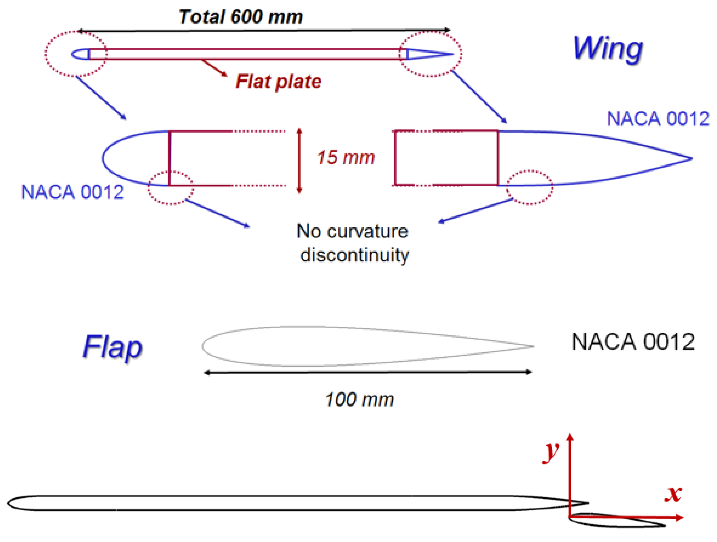
The full and detailed geometric model are sketched in Figure 1. The model is made up of NACA 0012 airfoils. The main wing is split at the max camber position and lengthened to 600 mm, while the chord length of the flap is 100 mm. The flow is three-dimensional in the (x, y, z) plane, where x is the freestream flow direction, y is the vertical flow direction, and z is the spanwise direction. x_flap and y_flap are coordinates of flap leading point (x_flap = 0 mm, y_flap = 0 mm), and the flaps can also be tilted at an angle_flap with respect to the z axis.
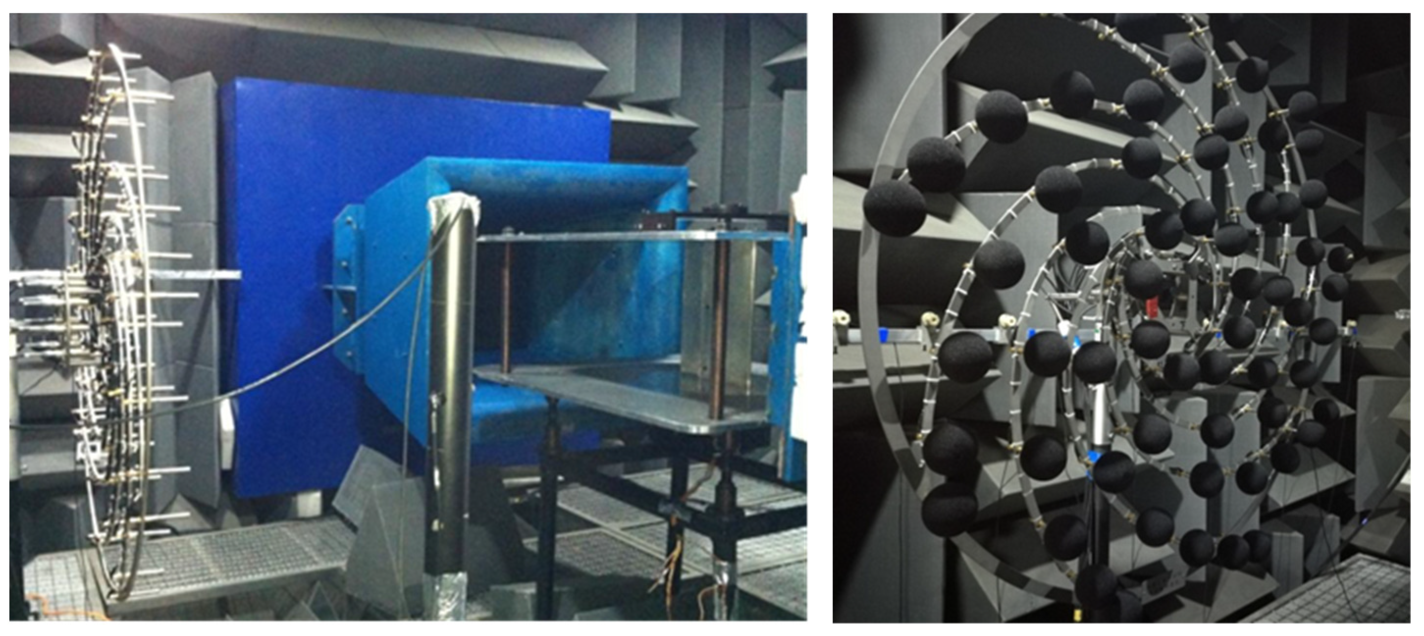
As shown in Figure 2, the model was installed in the middle of the side plates. The height of the plate is 375 mm (same as the test section), and the side plate is 900 mm wide and 970 mm long. The 63-channel phased array was utilized for far field directivity analysis. It is multispiral, and it has a radius of 1m. In the experiment, the phased array was placed 1.8 m away from the wind tunnel centerline.
The boundary conditions of the numerical simulation are obtained according to the experiment. The velocity of the freestream flow is U∞ = 50 m/s, the freestream temperature is T∞ = 300 K, and the static pressure is P∞ =101,325 Pa. The periodic conditions are set to the spanwise boundaries. The spanwise length is set as 0.4 chord length of the flap, which is 40 mm.
2.2. Numerical Algorithm
The three-dimensional Large Eddy Simulation (LES) equations [17,18] coupled with dynamic Smagorinsky subgrid model are employed for numerical simulation of the aerodynamics on wing and flap configuration. The commercial CFD program ANSYS FLUENT 19.1 is used to simulate the flow field. LES method directly calculates the turbulent motion larger than the grid scale through the unsteady Navier–Stokes (NS) equations, while the influence of small-scale vortices on large-scale vortices is reflected through subgrid model [19,20]. In LES method, two parts are divided for instantaneous variable φ, given by
where is the large-scale average component, which is processed using a filter function . D is the flow region, x is the spatial coordinate in the filtered large-scale space, x’ is the spatial coordinate in the actual flow region, and D (x, x’) determines the scale of the solved vortex. φ′ represents the small-scale components.
The unsteady NS equation is processed by the filter function , and the following can be obtained:
where τij is the subgrid scale stress, referred to as SGS stress, which reflects the influence of small-scale vortex motion on the NS equation. According to Smagorinsky model, SGS stress was given by
where is the turbulent viscosity at the sublattice scale.
where Δx represents the grid size along the x-axis, and CS is Smagorinsky constant.
The sound source term is calculated by unsteady CFD, and then the sound propagation characteristics are obtained by acoustic analogy method. The calculation methods of sound propagation characteristics mainly include Lighthill acoustic analogy equation [21], Curle’s acoustic analogy equation [22], FW–H acoustic analogy equation [23], and Kirchhoff integral method [24]. The FW–H acoustic analogy equation is used in present paper.
The FW–H acoustic analogy method is based on the near-field flow solution, which is used as the sound source signal, and the aerodynamic noise at the far-field observation point is obtained by integrating the FW–H formula, given by
where vn and un are the normal velocity of the control surface and the normal velocity of the fluid, H(f) is the Heaviside function, δ(f) Dirac function,
The solution of FW–H equation can be obtained:
The acoustic integral surface used in the integral formula can be any spatial surface containing solid. In this paper, the solid wing surface is taken as the integral surface, and the unsteady flow field information obtained by CFD simulation is taken as the input condition.
3. Numerical Validation
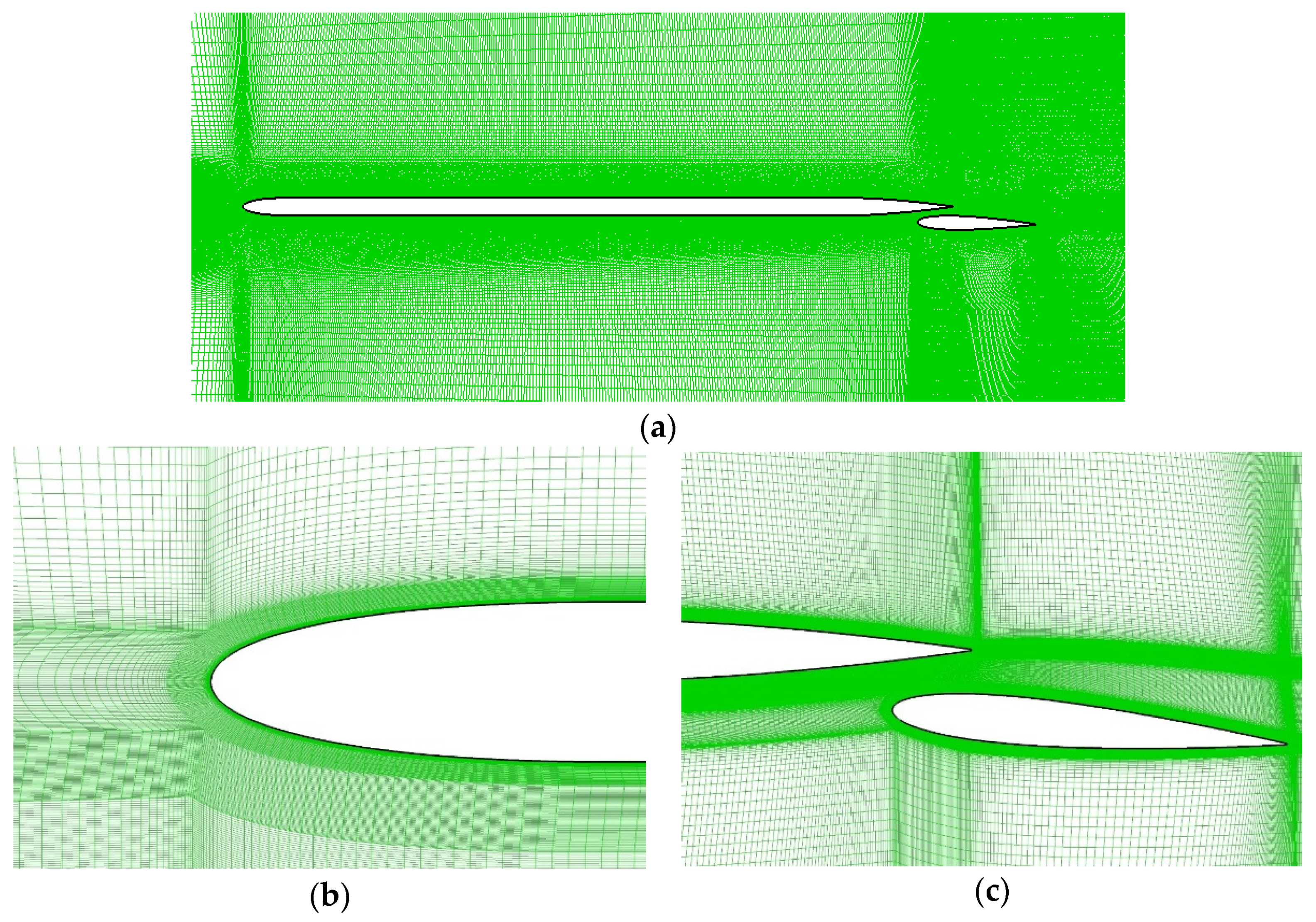
According to the experimental data performed by Bao [25] on pressure distribution, the numerical results obtained by CFD code are verified. Y+ is the main indicator for grid analysis, which plays an important role in turbulence modeling; it determines the height of the first cell normal to the wall. In this study, the height of the first cell is refined to obtain a Y+ value of approximately 1.0 to confirm the numerical accuracy. The X+ and Z+ estimations are 100 and 150 according to the length and width of the first cell, respectively. Similar grid scales can be referred to in the aerodynamic and aeroacoustics analysis of high-lift configuration using LES method [26]. The structural grids and the zoom-in view of the leading edge and trailing edge are shown in Figure 3. The parameters of mesh configuration are listed in Table 2.
In the numerical simulation, the implicit dual time-stepping approach was used to solve the unsteady flow field. To predict noise with frequency below 10 kHz in noise analysis, and according to the maximum frequency calculation formula F = 1/2Δt, the time step Δt was set to 5 × 10⁻⁵ s.
Comprehensively considering the computational accuracy and efficiency of numerical simulation, according to the research experience of relevant researchers [27], the spanwise width of the model was set to 0.4 times of the flap chord length.
The porous surface has an important influence on the analysis of noise [28]. Turbulence and vortices in the wake region are mainly quadrupole sound sources, which have little effect on the far-field noise at low speed. In this paper, the influence of dipole sound source is mainly considered, and the noise integral surface is directly taken on the solid wall.
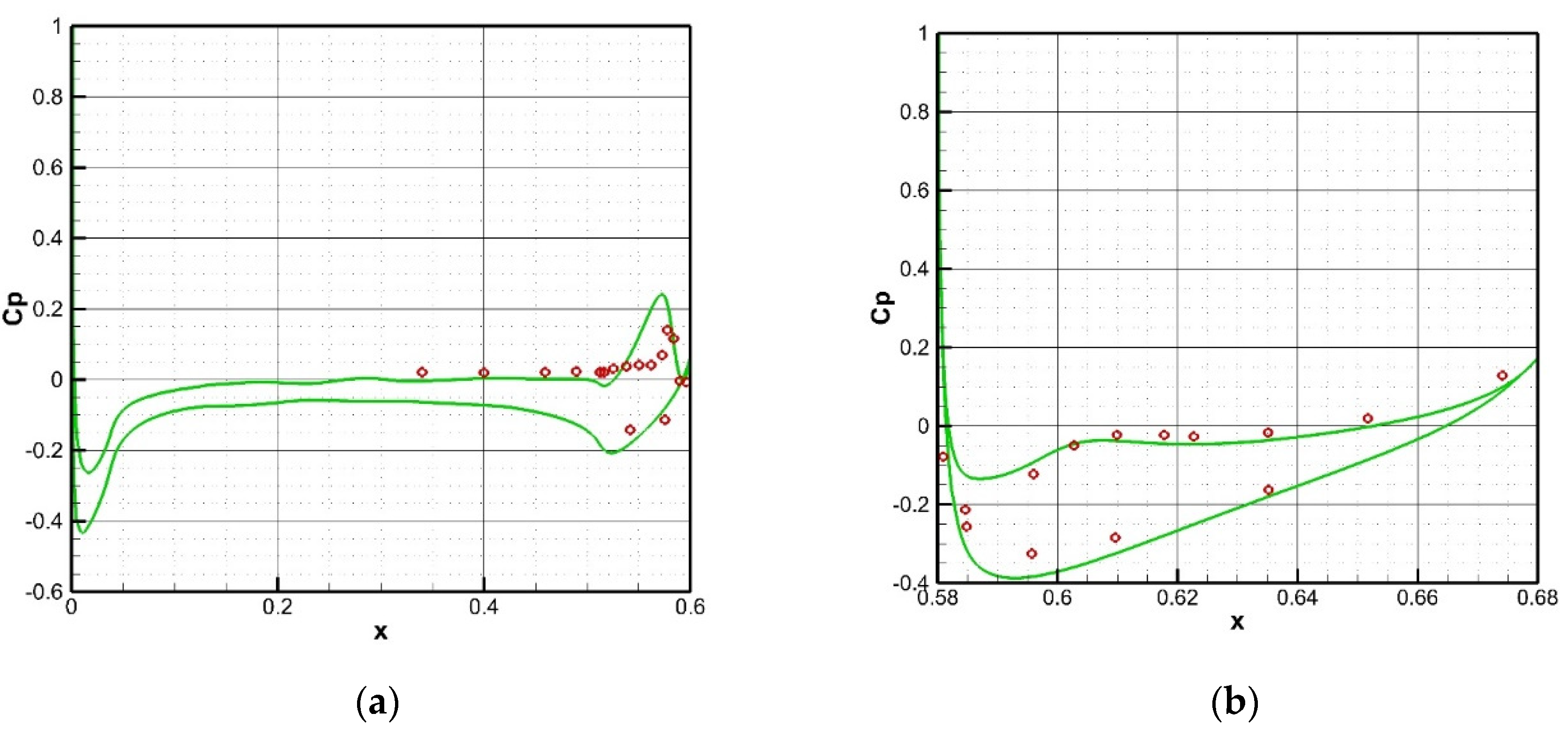
After the flow field is obtained by steady calculation, the mean values were obtained in last 5 s of the unsteady simulation process. The comparison of the mean pressure distributions along the surface between the numerical simulation and experimental results from the VALIANT database is presented in Figure 4. Figure 4a shows that there is a pressure rise at the upper trailing surface of the main wing, which is due to the block effect from the flap. Certain deviations could be observed here between the numerical results and experimental results, which could also be found in the research by Chalmers [29] and NUMECA [29]. Basically, the pressure coefficients on the surface of wing and flap from numerical simulations agree well with the experimental results.
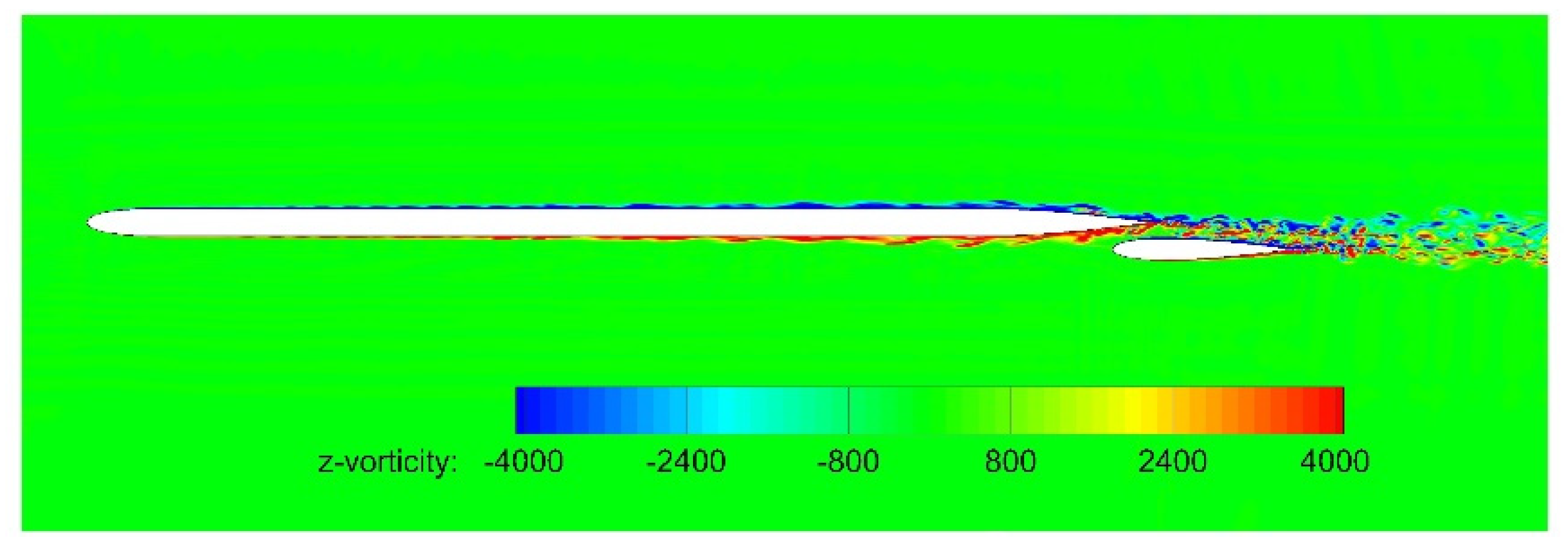
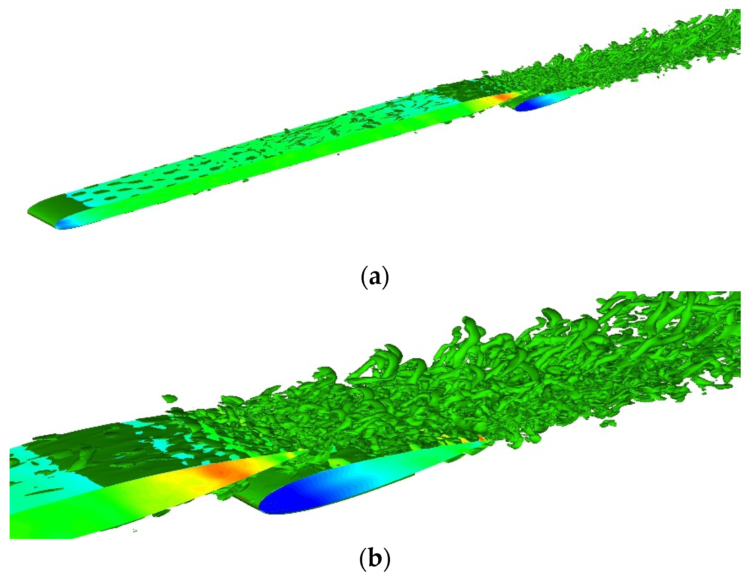
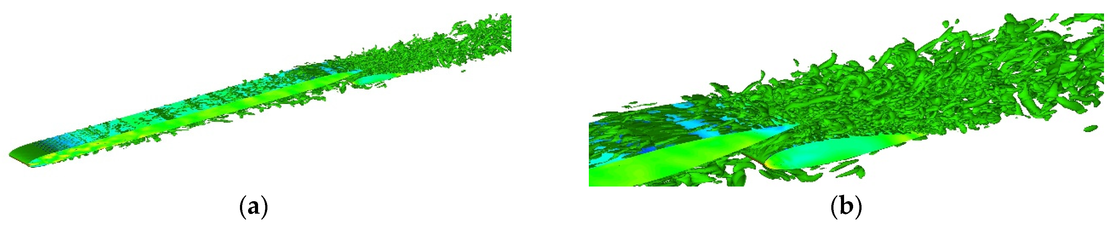
The z-direction vorticity contours calculated by the numerical approach are shown in Figure 5. Small vortex structures form at the regions where the pressure coefficient is high, and the flow becomes more chaotic. The wake of the wing has a great influence on the upper surface of the flap, which makes the flow on the upper surface of the airfoil separate rapidly. Figure 6 shows the iso-surfaces of Q-criterion. The vortex structures on the upper and lower surfaces of the airfoil are significantly less than that on the flap, since the flow on the airfoil surface is less disturbed and there is basically no flow separation. The vortex structures formed on the flap surface are relatively smaller compared to those over the main wing surface, indicating that the flap has more high-frequency noise sources relative to the main wing.
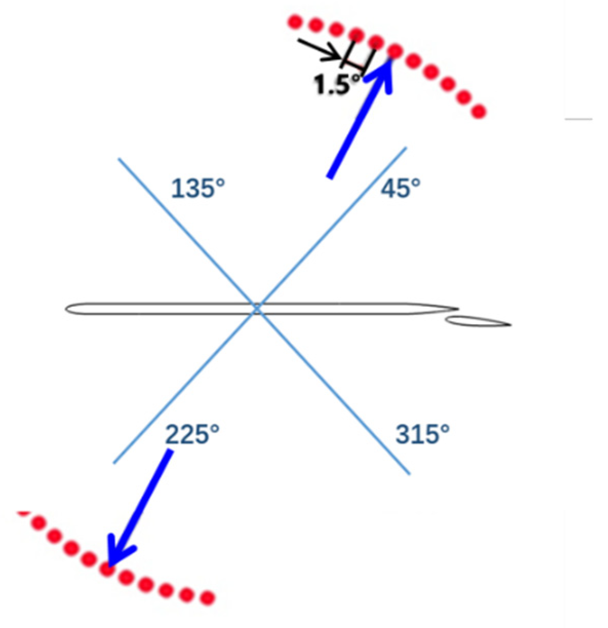
Microphones at 1.8 m from the middle of main wing on rotating support scan from 45° to 135° and 225° to 315°, while each set consists of 60 microphones with angle interval of 1.5°. The location of the probes in the far field is arranged according to the experiment, as shown in Figure 7.
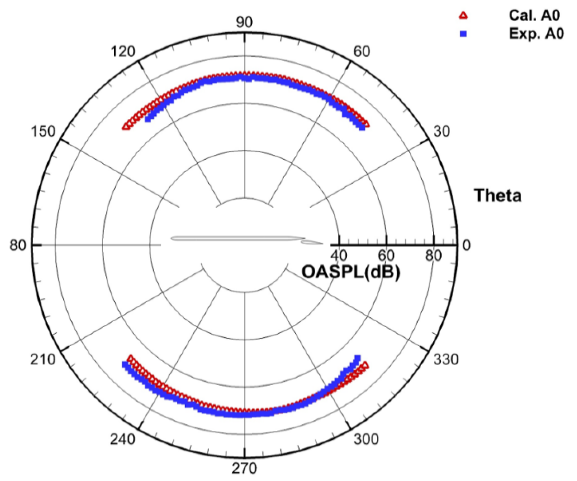
The overall sound pressure levels of the probes in the far field are shown in the figure below. According to Figure 8, the numerical simulation results agree well with experimental results, keeping the maximum error within 4 dB.
The characteristics of the flow field at 5° flap angle are also analyzed. The instantaneous contours of z-direction vorticity and the iso-surfaces of Q-criterion of the flow field at the 5° flap angle are shown in Figure 9 and Figure 10, respectively. The main flow structures are similar to that at the 0° flap angle. However, at the 5° flap angle, the shedding vortices at the trailing edge of the main wing and the flap have stronger interference, which makes the pressure in the passage between the main wing and the flap increase, and the backpressure gradient at the trailing edge of the main wing becomes stronger and the flow separation occurs. The deflection angle of the flap has a great influence not only on the flow around the flap, but also on the flow around the wing, especially on the flow around the lower surface of the wing.
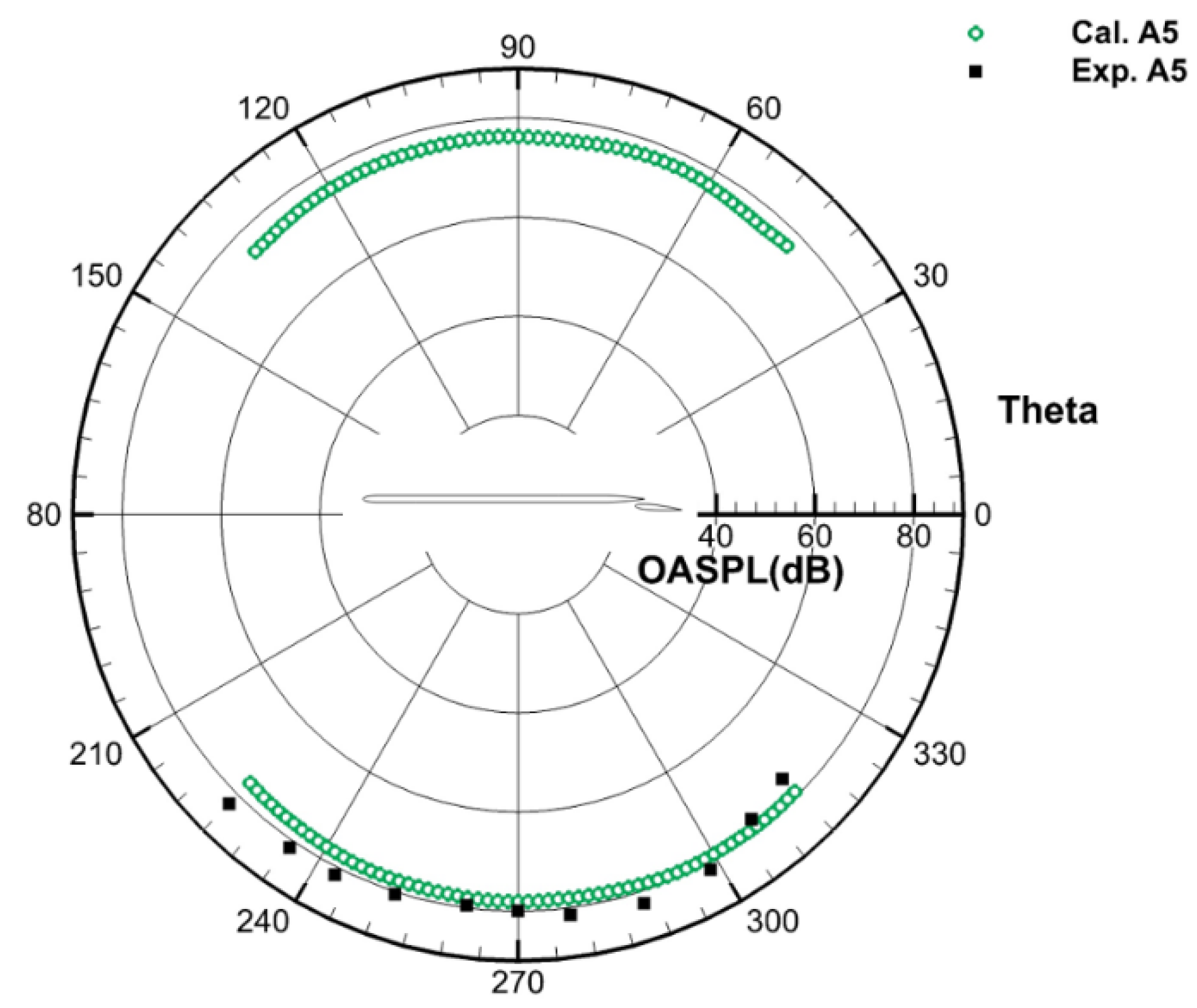
The overall sound pressure levels of the probes in the far field are shown in Figure 11. The experimental data only covers half of the far field noise (45~135°). The numerical predictions agree well with the experimental data, and the maximum error is kept within 4 dB.
4. Optimization Design Process and Results
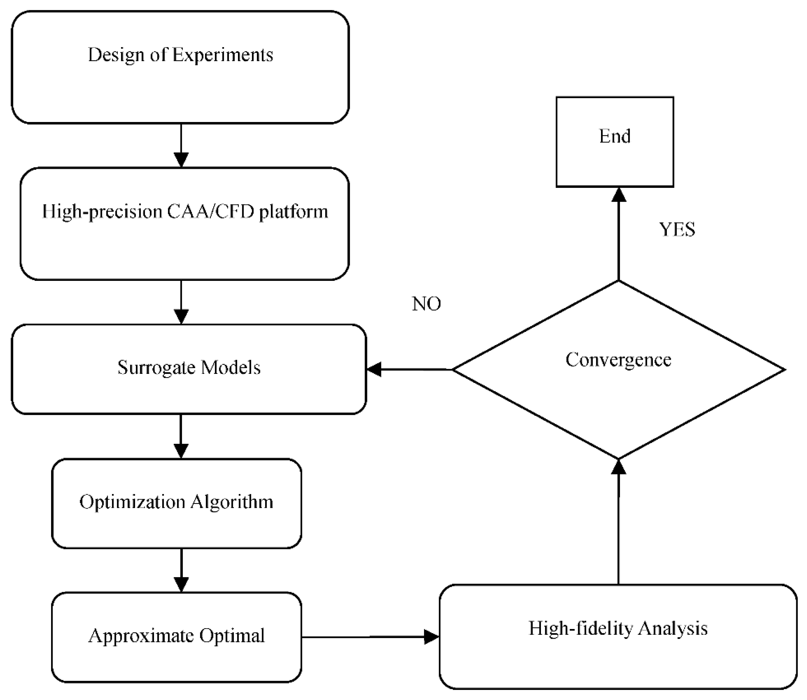
The surrogate-based optimization strategy consists of design of experiments, surrogate models and optimization algorithm [30]. The high-precision CAA/CFD platform coupled with surrogate model can effectively reduce the computational cost and improve the optimization efficiency [31]. The overall framework of the optimization process is shown in Figure 12.
4.1. Design Variables and Optimization Objectives
In current study, the optimization objective is to reduce the noise in the far field while the aerodynamic characteristics are maintained. The optimization variables are the flap position and the flap deflection. The flap position parameters should be included in selecting design variables. Coordinates of the flap leading point (x_flap, y_flap) and angle of the flap (angle_flap) are chosen as the design variables. Table 3 shows the design space.
The maximum overall sound pressure level (OASPL) of far-field noise is taken into consideration when selecting optimization objectives, as shown in Table 4.
The lift-drag ratio of the initial shape is 20.014. The aerodynamic loss is less than 1% after optimization, so the constraint condition is set to the lift-drag ratio of 19.814, as shown in Table 5.
4.2. Design of Experiments
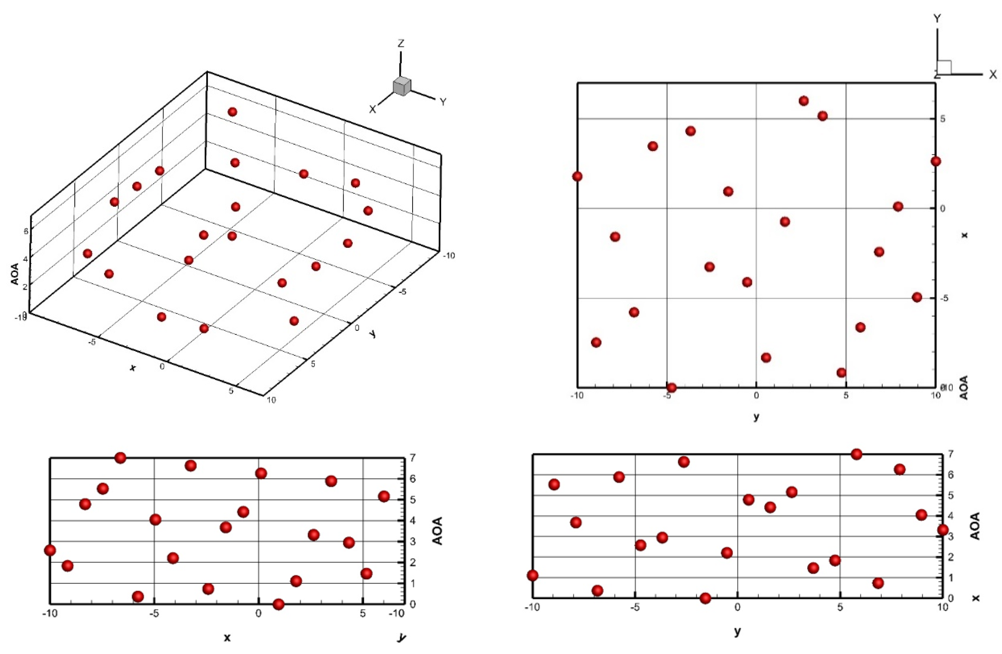
The experimental design method is a mathematical method about how to arrange experiments scientifically and reasonably [32]. It is a technology of arranging experiments economically and scientifically on the basis of probability theory and mathematical statistics [33]. In the present study, according to surrogate method and the computational cost, 19 samples of the three design variables are generated by Latin hypercube method. The distribution of sample points is shown in Table 6 and Figure 13. The design variables of sample points are uniformly distributed in the design space.
The relationship between design variable and objective function can be clarified by the scatter diagram between design variable and objective function [34,35]. Related tables and correlation maps can reflect the relationship between the two variables [36], but it is difficult to accurately show the degree of correlation between the two variables. The correlation coefficient is used to reflect the degree of linear correlation between two variables, which takes the form as
In which, Cov(X,Y) is the covariance of X and Y, Var[X] and Var[Y] are the variances of X and Y, respectively.
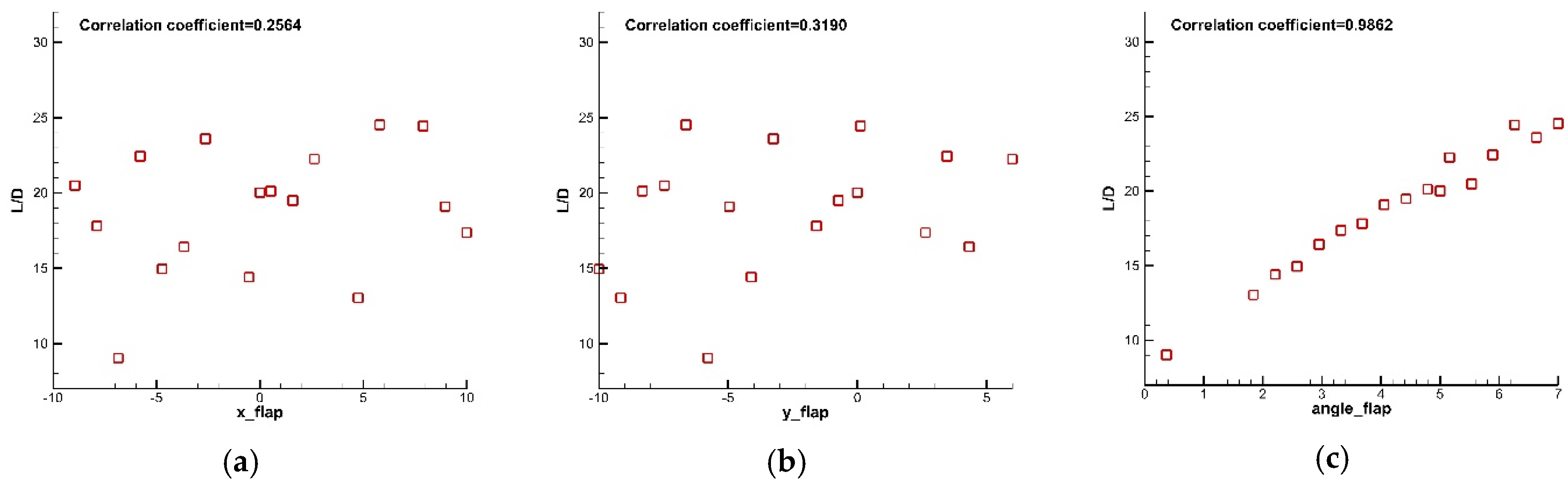
The scatter plots and correlation coefficients of three design variables (x_flap, y_flap, angle_flap) and lift-drag ratio (L/D) are given in Figure 14. In the scatter plots, the values of x-axis and y-axis represent the variation range of the two variables to be analyzed. The value of the correlation coefficient indicates the degree of linear correlation between the two variables, the closer the value of the correlation coefficient is to 1, the positive correlation between the two variables is shown. On the contrary, the closer the value of the correlation coefficient is to −1, the more the negative correlation between the two variables is shown. If the correlation coefficient is close to 0, the two variables have no linear correlation. In Figure 14a,b, the correlation coefficients are 0.2564 and 0.3190. The two design variables of x_flap and y_flap have positive correlation with lift-drag ratio (L/D). In Figure 14c, the correlation coefficient is 0.9862, indicating that the correlation between angle_flap and constraints is very strong.
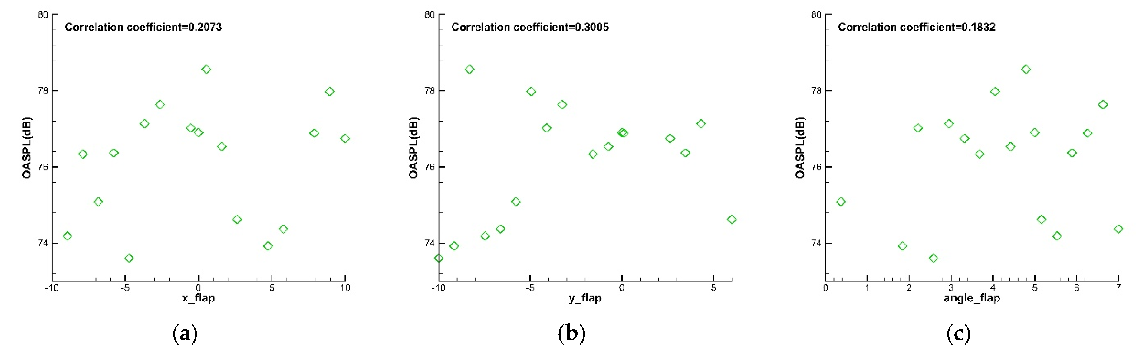
The scatter plots and correlation coefficients of three design variables (x_flap, y_flap, angle_flap) and the objectives (OASPL) are shown in Figure 15. The correlation coefficients are 0.2073, 0.3190, and 0.1832, respectively. The design variables of x_flap, y_flap, and angle_flap have positive correlation with the objectives. The scatter diagram shows that there is no linear correlation between variables.
4.3. The Surrogate Model
Kriging model [37] is an interpolation model for spatial modeling and prediction of random process/random field according to covariance function. Kriging model can obtain more accurate global optimal results than quadratic RSM model [38]. The model can be divided into regression model and correlation model. The regression model is the global approximation in the design space, and the correlation model can reflect the design spatial distribution structure of variables, which has an impact on the prediction accuracy of the model.
The Kriging model as a type of surrogate model can effectively establish a global mapping between design variables and optimization objectives, with lower computational cost. The Kriging surrogate model was widely used in aerodynamic design optimization of high-speed train [39] and high-lift airfoil design optimization [40].
4.4. Optimization Algorithm
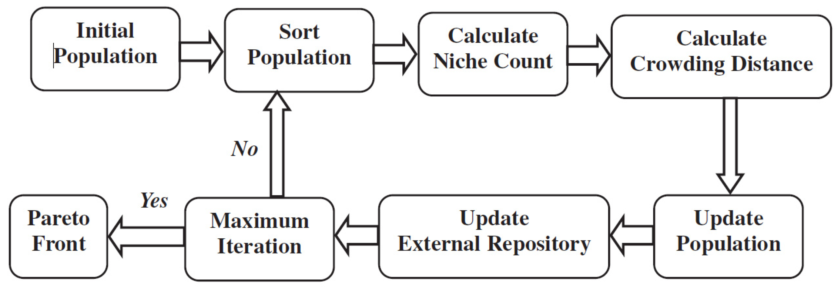
The particle swarm optimization algorithm (PSO) [41,42] is a famous design optimization algorithm that has good global optimization performance. Figure 16 shows the basic flow of a modified PSO algorithm by the authors [43]: first, the position and velocity of particles in the initial particle swarm are obtained by initializing the particle swarm. After that, the nondominated rank of the population is sorted by particle fitness. Then, the crowding distance of each particle and niche count can be obtained. The better progeny populations could be obtained, and the population could be updated.
4.5. Optimization Results
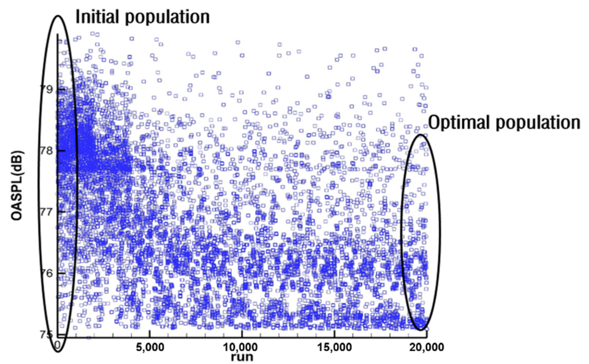
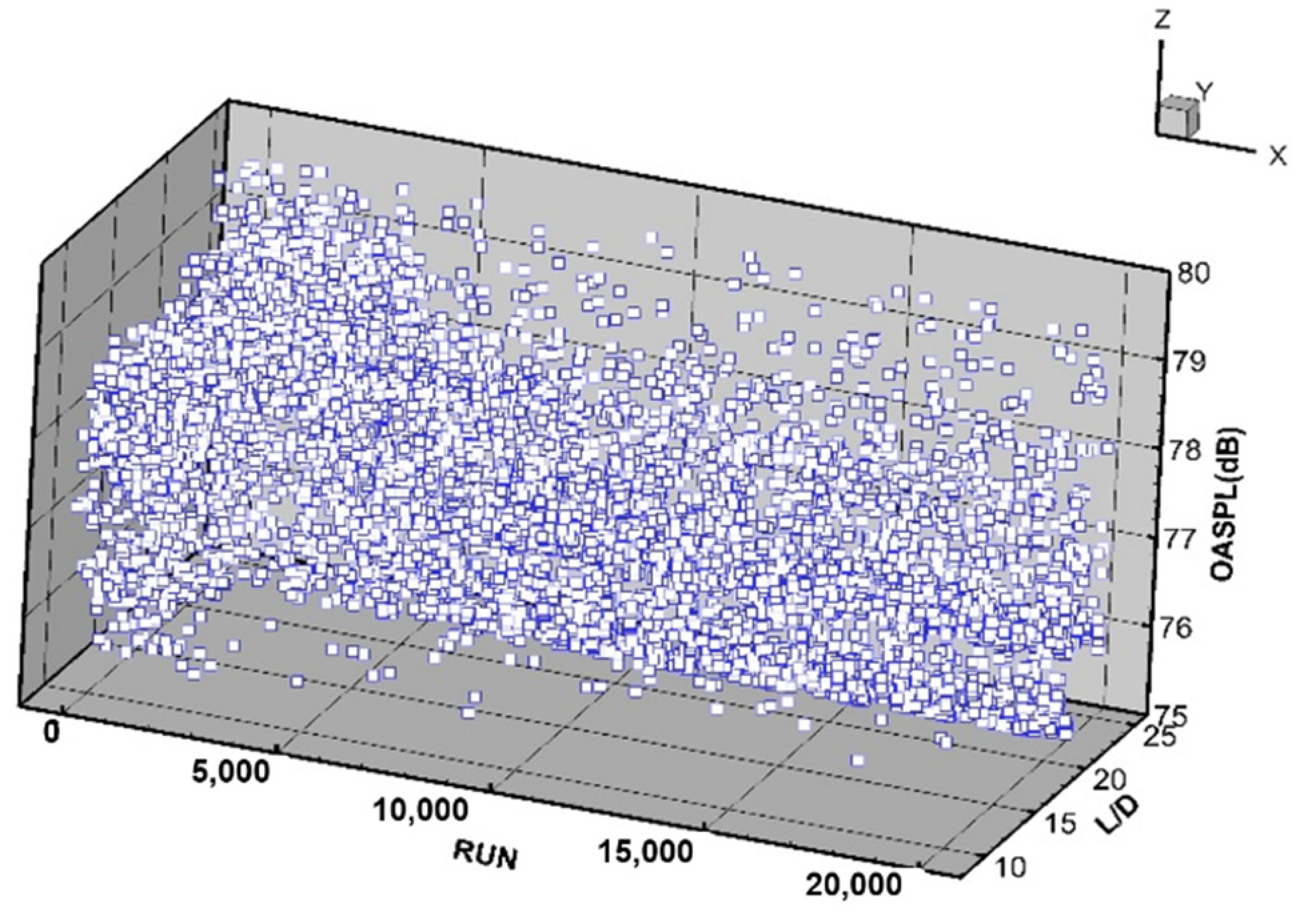
After adding sample points for three times, the optimization process is finished according to the progressive optimization strategy. And the evolutionary process of optimization objectives is shown in Figure 17. Overall sound pressure level (OASPL) values are dispersed, and the average value is larger in the initial population. With the optimization, the population of the OASPL improves, and the average value tends to converge. Therefore, the optimization design is carried out smoothly. Comparing further the optimization in the second and third rounds, there is little change in the optimal population of the two rounds.
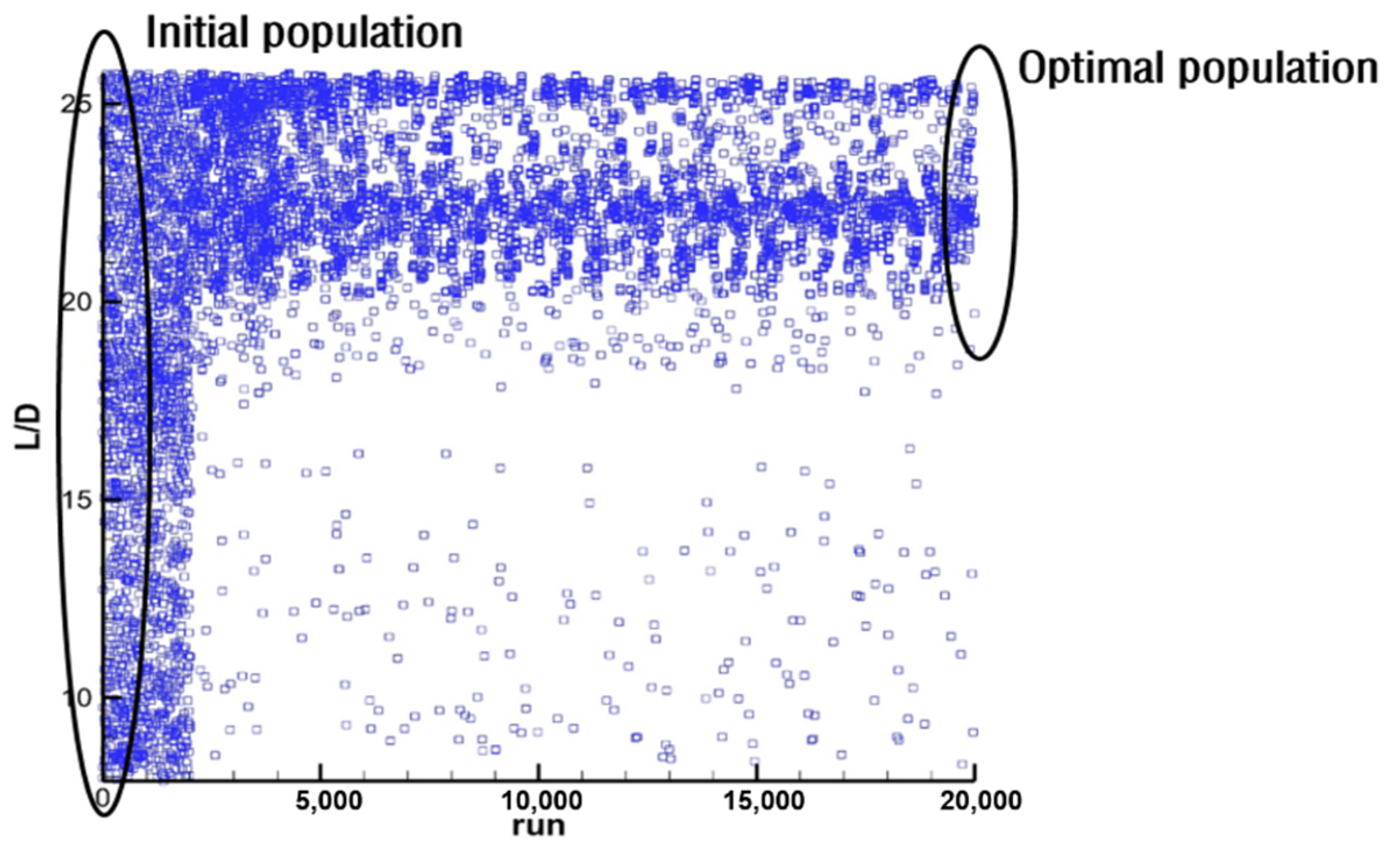
Figure 18 shows the variation of the constraints in the optimization process. The lift-drag ratio values are dispersed and the mean value is small in the initial population. With the second round of optimization, most of the lift-drag ratio values are larger than the constraints and the mean value tends to converge.
The variation of overall sound pressure level (OASPL) values and lift-drag ratio (L/D) values with the optimization iteration are shown in Figure 19. With the optimization proceeding, the evolutionary tendency of the population becomes smaller and converges.
After the three rounds of optimization design, the configuration parameters of the optimized shape are compared with those of the initial shape, as shown in Table 7. With the constraint of L/D ratio, there is little change on the flap deflection angle. After the change of the position of the flap, the width of the channel between the flap and the wing changes, so the effect of reducing noise is realized.
The optimization results are validated by CFD/CAA, as shown in Table 8. The errors of OASPL value and lift-drag ratio value between the two models are small, which verifies the accuracy of the surrogate model and the correctness of the optimization method.
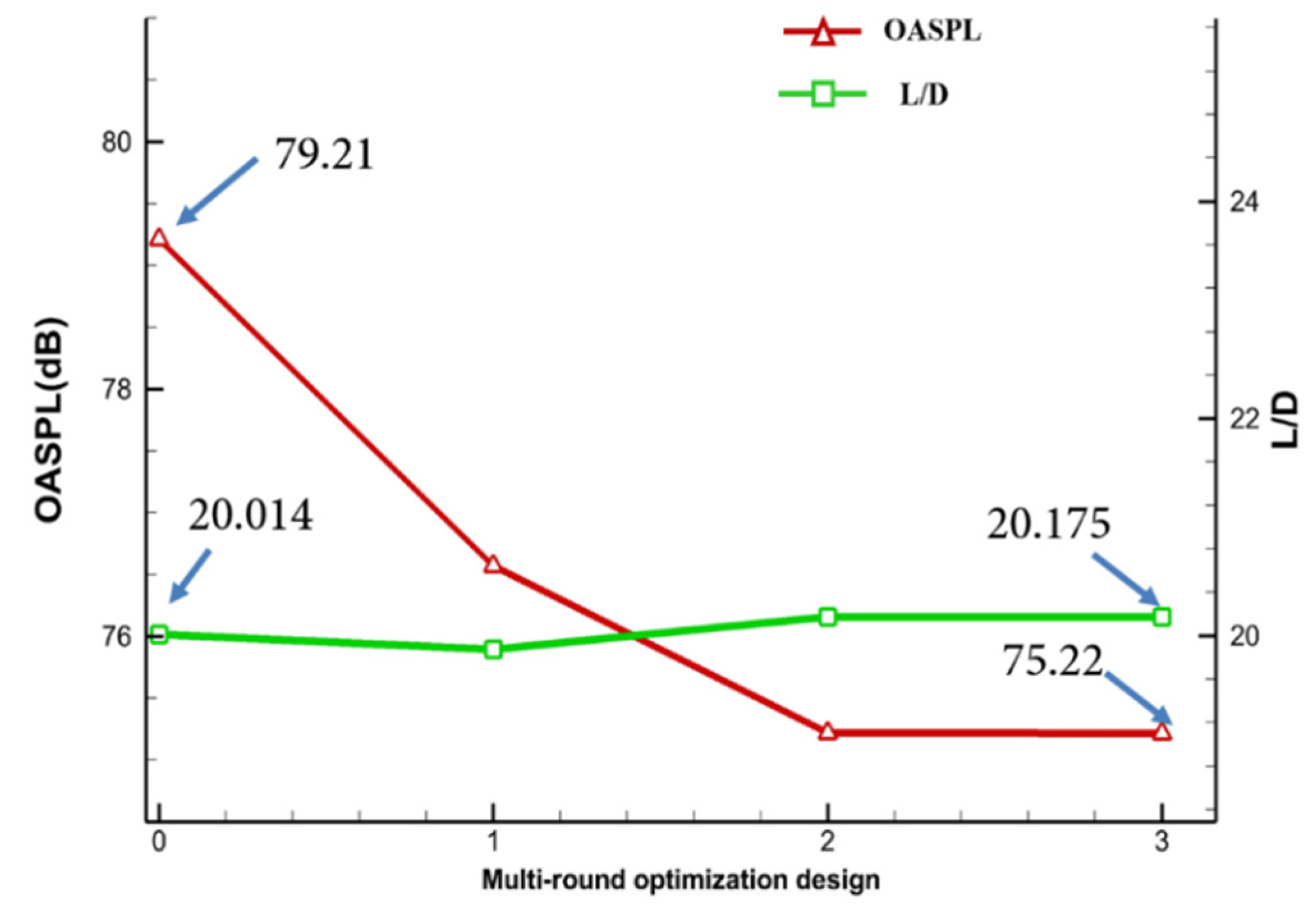
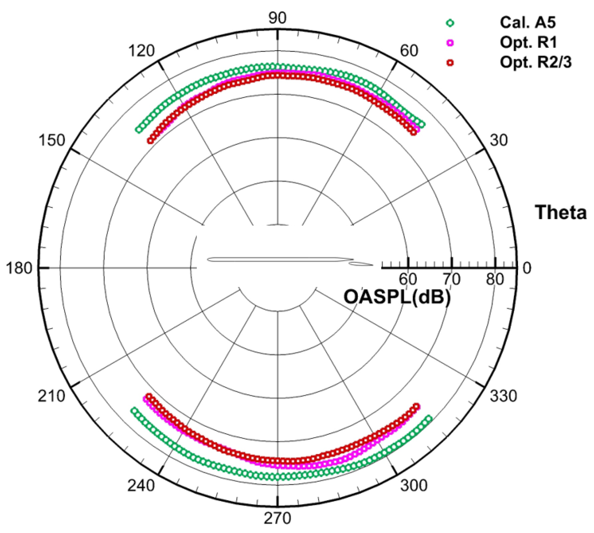
Figure 20 gives the converging process of the optimization objectives in the three-round optimization design. Comparing the results of aerodynamic performance and aerodynamic noise between the initial shape and the optimized shape, the maximum far-field total sound pressure level value of the optimized shape decreases by 3.99 dB, and the lift-drag ratio value increases by 0.8%. The comparison of the far-field OASPLs before and after the optimization is given in Figure 21. After the three-round optimization design, the optimization results tend to converge and satisfy the constraints.
4.6. Discussions
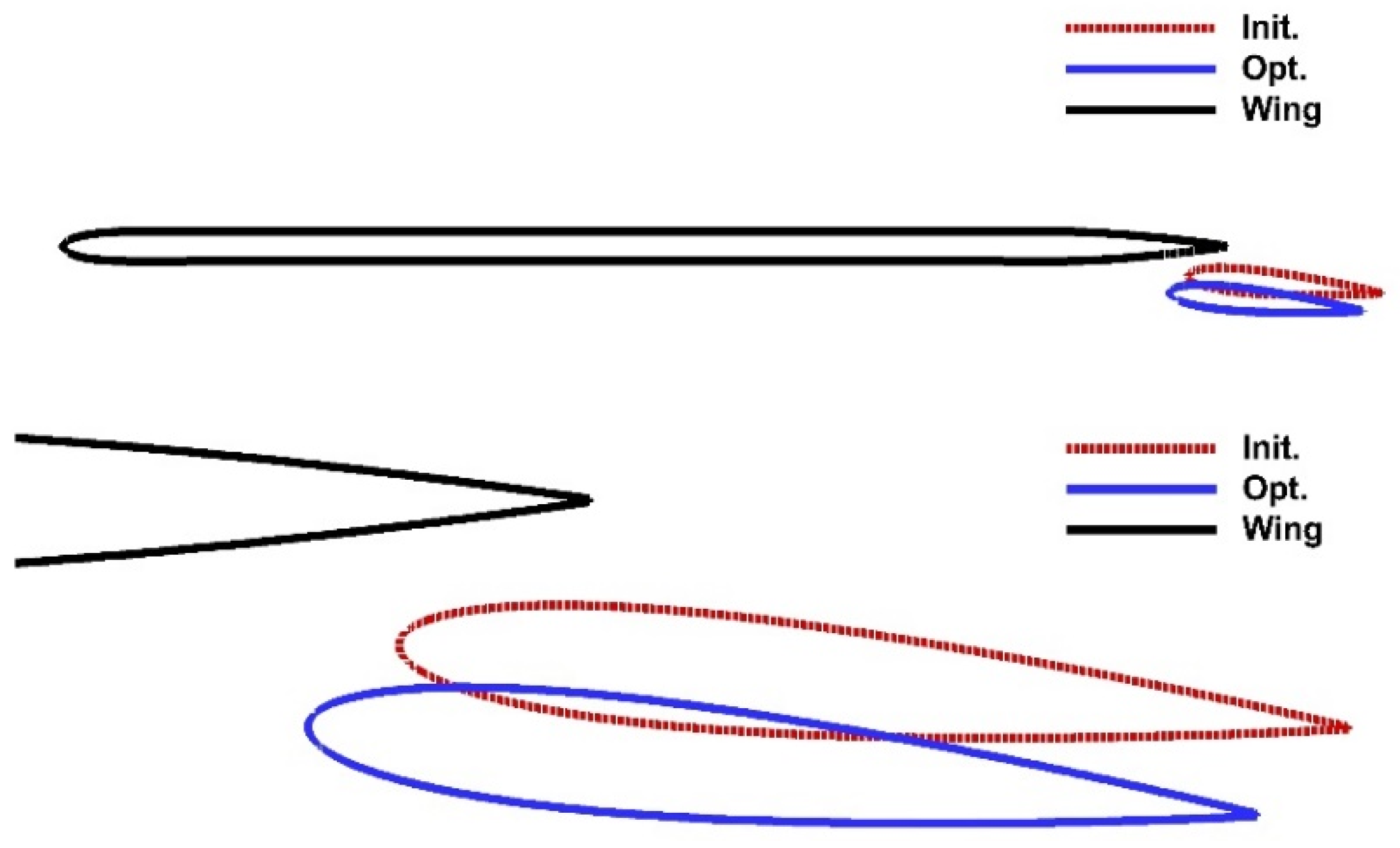
Aiming at the change of flow field caused by the shape variation, the optimal design results are discussed. Figure 22 shows the comparison between the initial shape and the optimal shape. In the x-axis direction, the flap leading edge of the optimal shape is close to the leading edge of the main wing, and the flap leading edge of the optimized shape is downward, which widens the channel between the flap and the main wing, and the deflection angle of the optimal shape is almost unchanged compared with that of the initial shape.
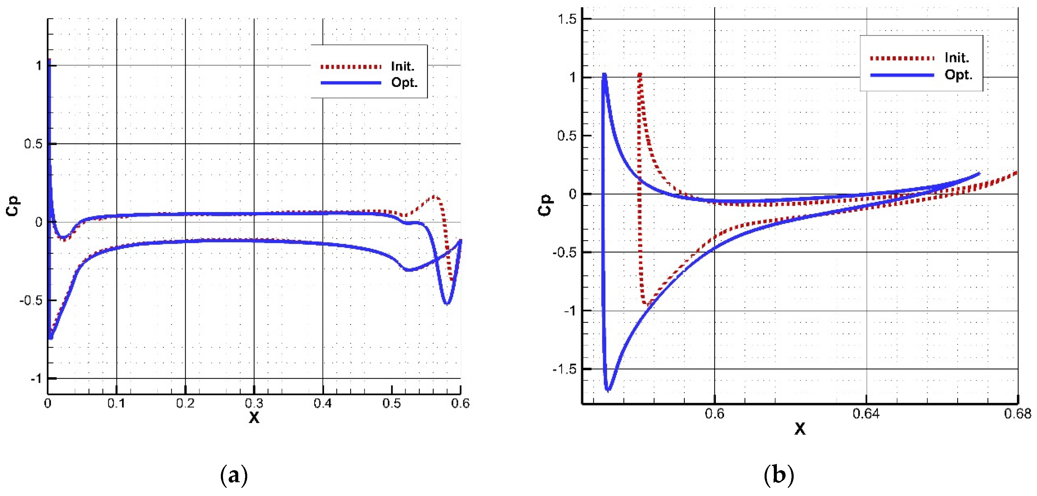
The pressure coefficients on the airfoil surface before and after optimization are shown in Figure 23. For the upper surface of the main wing, the pressure coefficients of the optimal airfoil are almost the same as that of the original airfoil. At the lower trailing edge of the main wing, the pressure coefficients of the optimized airfoil decrease compared with the initial airfoil, and the area of the inverse pressure gradient decreases. Thus, the interference between main wing and flap is reduced. The flap has a limited influence on the wing, and there is no change on the pressure in front of the wing.
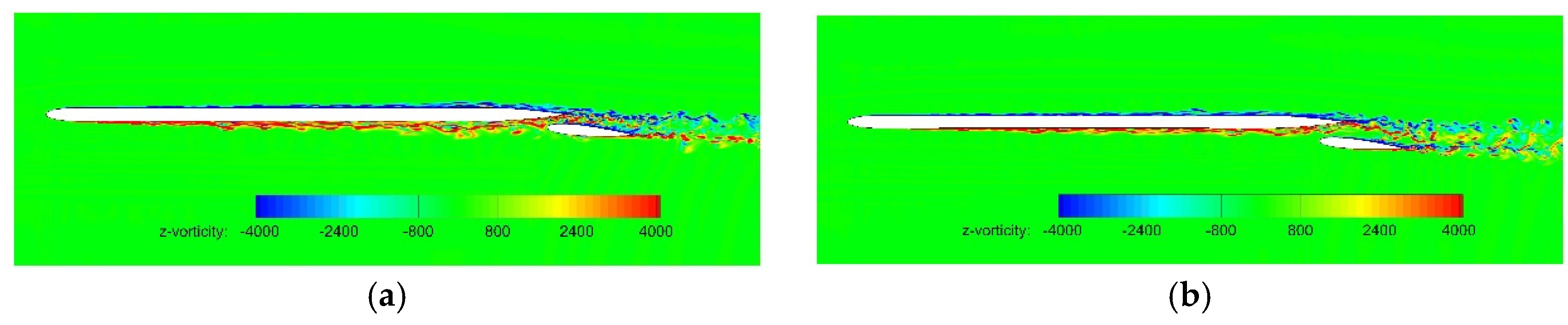
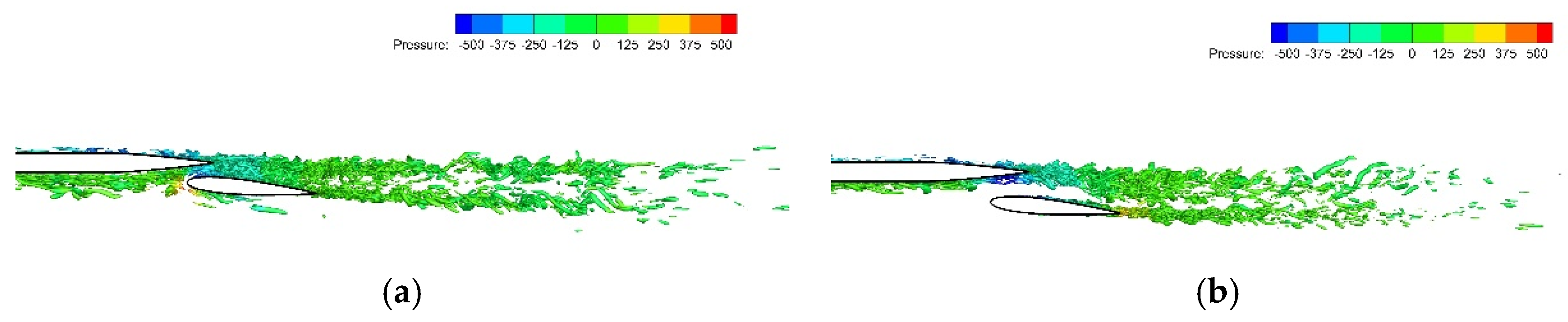
The z-direction vorticity contours and the iso-surfaces of Q-criterion (Q = 5000) of the initial shape and the optimal shape are shown in Figure 24 and Figure 25. The difference between the flow field of the optimal shape and that of the initial shape is mainly reflected in the gap between the main wing and the flap. After optimization, the area of the inverse pressure gradient region on the main wing surface is reduced, and more air flow can pass by the passage between the main wing and the flap. The passage between the main wing and the flap becomes wider and the blocking effect of the flow is reduced and the separation area at the tail of the main wing is significantly reduced. Consequently, the aerodynamic noise is also reduced.
5. Conclusions
In this paper, the particle swarm optimization algorithm combined with Kriging surrogate model is applied to optimize the flap position parameters of three-dimensional wing and flap configuration. The aerodynamic and aeroacoustic predictions are calculated by numerically solving Large Eddy Simulation (LES) equations with Ffowcs–William and Hawkings (FW–H) equation. In the optimization, coordinates of the flap leading point (x_flap, y_flap) and angle of the flap (angle_flap) were taken as the design variables, and the maximum overall sound pressure level (OASPL) of far-field noise were set as the objective function. The following conclusions are drawn:
- (a)
- The numerical results of three-dimensional wing and flap configuration show reasonable agreement with the experimental data. Thus, the aerodynamic noise of a simplified wing model can be accurately assessed by means of high-fidelity CAA/CFD numerical simulation.
- (b)
- The relationships between the design variables and the objectives were analyzed by correlation coefficients and scatter plots. The two design variables of x_flap and y_flap have positive correlation with the maximum OASPL and the lift-drag ratio (L/D). Meanwhile, a strong correlation exists between angle_flap and L/D.
- (c)
- Under aerodynamic constraints, the maximum overall sound pressure level is reduced by 3.99dB after optimization. At the same time, the optimized values of x_flap and y_flap are located near the lower limit value, while the optimized values of angle_flap are located in the middle part over the range.
- (d)
- With the deflection angle of the flap almost unchanged, the aerodynamic noise can be reduced, while ensuring a large L/D by changing the positional relationship between the flap and the main wing. The research results can provide suggestions for the design of low-noise & high-lift configuration, as well as their application in high-lift devices.
Author Contributions
Methodology, S.J. and Z.S.; validation, Y.W. and C.Y.; formal analysis, S.J. and Z.S.; investigation, D.G. and G.Y. All authors have read and agreed to the published version of the manuscript.
Funding
This work is supported by the Youth Innovation Promotion Association CAS (2019020) and the EU-China IMAGE project (Grant No. 688971). Innovative Methodologies and technologies for reducing Aircraft noise Generation and Emission (IMAGE) is an EU-China collaborative project between a European team (Chalmers, AGI, CFDB, CIMNE, KTH, NLR, NUMECA, ONERA, RWTH-Aachen, TU-K, UPM, and VKI) and a Chinese team (ASRI, ACAE, ARI, BASTRI, BUAA, FAI, IMech, NPU, and THU).
Institutional Review Board Statement
Not applicable.
Informed Consent Statement
Not applicable.
Data Availability Statement
Not applicable.
Acknowledgments
The Computing Facility for the “Era” petascale supercomputer of the Computer Network Information Center of the Chinese Academy of Sciences is gratefully acknowledged.
Conflicts of Interest
The authors declare no conflict of interest.
References
- Dobrzynski, W. Almost 40 Years of Airframe Noise Research: What Did We Achieve? J. Aircr. 2010, 47, 353–367. [Google Scholar] [CrossRef]
- Envia, E.; Thomas, R. Recent Progress in Aircraft Noise Research. In Aeronautics Research Mission Directorate (ARMD) Technical Seminar; NASA Glenn Research Center: Cleveland, OH, USA, 2007. [Google Scholar]
- Choudhari, M.M.; Khorrami, M.R. Slat Cove Unsteadiness: Effect of 3D Flow Structures. In Proceedings of the 44th AIAA Aerospace Sciences Meeting and Exhibit, Reno, NV, USA, 9–12 January 2006. [Google Scholar]
- Takeda, K.; Ashcroft, G.; Zhang, X.; Nelson, P. Unsteady aerodynamics of flap cove flow in a high-lift device configuration. In Proceedings of the 39th Aerospace Sciences Meeting and Exhibition, Reno, NV, USA, 8–11 January 2001. [Google Scholar]
- Fink, M.R.; Schlinke, R.H. Airframe Noise Component Interaction Studies. J. Aircr. 1980, 17, 99–105. [Google Scholar] [CrossRef] [Green Version]
- Ahtye, W.F.; Miller, W.R.; Meecham, W.C. Wing and Flap Noise Measured by Near- and Far-Field Cross-Correlation Techniques; AIAA: Reston, VA, USA, 1979; pp. 1–14. [Google Scholar]
- Miller, W.R.; Meecham, W.C.; Ahtye, W.F. Large scale model measurements of airframe noise using cross-correlation techniques. J. Acoust. Soc. Am. 1982, 66, 591–599. [Google Scholar] [CrossRef]
- Khorrami, M.R.; Berkman, M.E.; Choudhari, M. Unsteady Flow Computations of a Slat with a Blunt Trailing Edge. AIAA J. 2000, 38, 2050–2058. [Google Scholar] [CrossRef]
- Streett, C.L. Numerical Simulation of Fluctuations Leading to Noise in a Flap-Edge Flowfield. In Proceedings of the 36th AIAA Aerospace Sciences Meeting and Exhibit, Reno, NV, USA, 12–15 January 1998. [Google Scholar]
- Radeztsky, R.; Singer, B. Detailed measurements of a flap side-edge flow fie. In Proceedings of the 36th AIAA Aerospace Sciences Meeting and Exhibit, Reno, NV, USA, 12–15 January 1998. [Google Scholar]
- Rackl, R.G.; Miller, G.; Guo, Y.; Yamamoto, K. Airframe Noise Studies: Review and Future Direction; NASA: Washington, DC, USA, 2005. [Google Scholar]
- Ge, M.M.; Wang, S.Y.; Wang, G.X.; Deng, X.G. Aeroacoustic simulation of the high-lift airfoil using hybrid reynolds averaged Navier-Stokes/high-order implicit large eddy simulation method. Acta Phys. Sin. 2019, 68, 204702. [Google Scholar] [CrossRef]
- Satti, R.; Li, Y.; Shock, R.; Noelting, S. Aeroacoustic Analysis of a High Lift Trapezoidal Wing Using Lattice Boltzmann Method. In Proceedings of the 14th AIAA/CEAS Aeroacoustics Conference (29th AIAA Aeroacoustics Conference), Vancouver, BC, Canada, 5–7 May 2008. [Google Scholar]
- Dong, T.; Reddy, N.; Tam, C. Direct numerical simulations of flap side edge noise. In Proceedings of the 5th AIAA/CEAS Aeroacoustics Conference and Exhibit, Bellevue, WA, USA, 10–12 May 1999. [Google Scholar]
- Rakhshani, B.; Filippone, A. Noise from High-Lift Leading-Edge Device. In Proceedings of the 24th AIAA Applied Aerodynamics Conference, San Francisco, CA, USA, 5–8 June 2006. [Google Scholar]
- Yann, D.; Ronith, S.; Steven, H.F.; David, G. Application of Actuator Line Model for Large Eddy Simulation of Rotor Noise Control. Aerosp. Sci. Technol. 2021, 108, 106405. [Google Scholar]
- Boudet, J.; Grosjean, N.; Jacob, M. Wake-airfoil interaction as broadband noise source: A large-eddy simulation study. Int. J. Aeroacoustics 2009, 4, 93–116. [Google Scholar] [CrossRef]
- Wagner, C.; Hüttl, T.; Sagaut, P. (Eds.) Large-Eddy Simulation for Acoustics; Cambridge University Press: Cambridge, MA, USA, 2007. [Google Scholar]
- Ju, S.; Yan, C.; Wang, X.; Qin, Y.; Ye, Z. Optimization design of energy deposition on single expansion ramp nozzle. Acta Astronaut. 2017, 140, 351–361. [Google Scholar] [CrossRef]
- Ju, S.; Yan, C.; Wang, X.; Qin, Y.; Ye, Z. Effect of energy addition parameters upon scramjet nozzle performances based on the variance analysis method. Aerosp. Sci. Technol. 2017, 70, 511–519. [Google Scholar] [CrossRef]
- Lighthill, M.J. On Sound Generated Aerodynamically I. General Theory. Proc. R. Soc. Lond. Ser. A 1951, 211, 564–587. [Google Scholar]
- Curle, N. The Influence of Solid Boundaries Upon Aerodynamic Sound. Proc. R. Soc. A Math. Phys. Sci. 1955, 231, 505–514. [Google Scholar]
- Williams, J.F.; Hawkings, D.L. Sound Generation by Turbulence and Surfaces in Arbitrary Motion. Philos. Trans. R. Soc. Lond. Ser. A Math. Phys. Sci. 1969, 264, 321–342. [Google Scholar]
- Kirchhoff, G.R. Zur Theorie der Lichtstrahlen. Annalen Der Physik 2010, 254, 663–695. [Google Scholar] [CrossRef] [Green Version]
- Bao, A.Y.; Ding, C.W.; Zhou, G.C.; Chen, B. Wind tunnel test study on aerodynamic noise control method of lifting device. In Innovation and Development of Green Aviation Technology; Aviation Industrial Publishing House: Beijing, China, 2020. [Google Scholar]
- Lu, Q.; Chen, B. Analysis of aeroacoustics characteristics of high lift device using LES method. Acta Aerodyn. Sin. 2016, 34, 448–455. [Google Scholar]
- Giret, J.C.; Sengissen, A.; Moreau, S.; Sanjosé, M.; Jouhaud, J.C. Prediction of the Sound Generated by a Rod-airfoil Configuration Using a Compressible Unstructured LES Solver and a FW-H Analogy. In Proceedings of the 18th AIAA/CEAS Aeroacoustics Conference Colorado, Springs, CO, USA, 4–6 June 2012. [Google Scholar]
- Testa, C.; Porcacchia, F.; Zaghi, S.; Gennaretti, M. Study of a FWH-based permeable-surface formulation for propeller hydroacoustics. Ocean. Eng. 2021, 240, 109828. [Google Scholar] [CrossRef]
- Xiao, Z.; Zhu, W.; Fu, S. CFD/CAA analysis of noise generation, propagation and control. In Innovation and Development of Green Aviation Technology; Aviation Industrial Publishing House: Beijing, China, 2020. [Google Scholar]
- Ju, S.; Sun, Z.; Yang, G.; Prapamonthon, P.; Zhang, J. Multi-objective design optimization of the combinational configuration of the upstream energy deposition and opposing jet for drag reduction in supersonic flows. Aerosp. Sci. Technol. 2020, 105, 105941. [Google Scholar] [CrossRef]
- Sun, Z.; Song, J.; An, Y. Optimization of the head shape of the CRH3 high speed train. Sci. China Technol. Sci. 2010, 53, 3356–3364. [Google Scholar] [CrossRef]
- Wang, G.G. Adaptive Response Surface Method Using Inherited Latin Hypercube Design Points. J. Mech. Des. 2003, 125, 210–220. [Google Scholar] [CrossRef]
- Ju, S.; Yan, C.; Wang, X.; Qin, Y.; Ye, Z. Sensitivity analysis of geometric parameters upon the aerothermodynamic performances of Mars entry vehicle. Int. J. Heat Mass Transf. 2018, 120, 597–607. [Google Scholar] [CrossRef]
- Yang, G.; Guo, D.; Yao, S.; Liu, C. Aerodynamic design for China new high-speed trains. Sci. China Technol. Sci. 2012, 55, 1923–1928. [Google Scholar] [CrossRef] [Green Version]
- Yang, G.; Chen, D.; Cui, K. Response Surface Technique for Static Aeroelastic Optimization on a High-Aspect-Ratio Wing. J. Aircr. 2009, 46, 1444–1450. [Google Scholar] [CrossRef]
- Cornell, J.A. Factors that influence the value of the coefficient of determination in simple linear and nonlinear regression models. Phytopathology 1987, 77, 63–70. [Google Scholar] [CrossRef]
- Koehler, J.R.; Owen, A.B. Computer experiments. In Handbook of Statistics; Ghosh, S., Rao, C.R., Eds.; Elsevier Science: New York, NY, USA, 1996; pp. 261–308. [Google Scholar]
- Welch, W.J.; Yu, T.K.; Kang, S.M.; Sacks, J. Computer experiments for quality control by parameter design. J. Qual. Technol. 1990, 22, 15–22. [Google Scholar] [CrossRef]
- Xu, L.; Zhang, B.; Chen, B.; Wu, P. Multi-Objective Optimization Design of Liftbody Aircraft Using Kriging Model. J. Phys. Conf. Ser. 2021, 1985, 012034. [Google Scholar] [CrossRef]
- Zhang, L.; Zhang, J.Y.; Li, T.; Zhang, Y.D. Multi-objective aerodynamic optimization design of high-speed train head shape. J. Zhejiang Univ.-Sci. A 2017, 18, 841–854. [Google Scholar] [CrossRef]
- Fourie, P.C.; Groenwold, A.A. The particle swarm optimization algorithm in size and shape optimization. Struct. Multidiscip. Optim. 2002, 23, 259–267. [Google Scholar] [CrossRef]
- Khan, T.A.; Ling, S.H. A novel hybrid gravitational search particle swarm optimization algorithm. Eng. Appl. Artif. Intell. 2021, 102, 104263. [Google Scholar] [CrossRef]
- Yao, S.; Guo, D.; Sun, Z.; Yang, G. A modified multi-objective sorting particle swarm optimization and its application to the design of the nose shape of a high-speed train. Eng. Appl. Comput. Fluid Mech. 2015, 9, 513–527. [Google Scholar] [CrossRef] [Green Version]
Figure 1.
Schematic diagram of wing and flap configuration.

Figure 2.
Anechoic wind tunnel and 63-channel phased array for experiment.

Figure 3.
Structural meshes of wing and flap configuration: (a) the whole view; (b) zoom-in view near the leading edge; (c) zoom-in view near the flap.
Figure 3.
Structural meshes of wing and flap configuration: (a) the whole view; (b) zoom-in view near the leading edge; (c) zoom-in view near the flap.

Figure 4.
Comparing results between numerical simulation and experiment: on main wing (a); on flap (b).
Figure 4.
Comparing results between numerical simulation and experiment: on main wing (a); on flap (b).

Figure 5.
z-direction vorticity contours.

Figure 6.
Iso-surfaces of Q-criterion (Q = 5000) for the case with the deflection angle of 0°: (a) the whole view; (b) zoom-in view near the flap.
Figure 6.
Iso-surfaces of Q-criterion (Q = 5000) for the case with the deflection angle of 0°: (a) the whole view; (b) zoom-in view near the flap.

Figure 7.
Microphone array for far-field measurements.

Figure 8.
Sound pressure levels of probes in far field.

Figure 9.
z-direction vorticity contours.

Figure 10.
Iso-surfaces of Q-criterion (Q = 5000) for the case with the deflection angle of 0°: (a) the whole view; (b) zoom-in view near the flap.
Figure 10.
Iso-surfaces of Q-criterion (Q = 5000) for the case with the deflection angle of 0°: (a) the whole view; (b) zoom-in view near the flap.

Figure 11.
Sound pressure levels of far field probes.

Figure 12.
Framework of optimization process.

Figure 13.
Distribution of sample points.

Figure 14.
Scatter plots of L/D versus x_flap (a); Scatter plots of L/D versus y_flap (b) Scatter plots of L/D versus angle_flap (c).
Figure 14.
Scatter plots of L/D versus x_flap (a); Scatter plots of L/D versus y_flap (b) Scatter plots of L/D versus angle_flap (c).

Figure 15.
Scatter plots of OASPL versus x_flap (a); Scatter plots of OASPL versus y_flap (b) Scatter plots of OASPL versus angle_flap (c).
Figure 15.
Scatter plots of OASPL versus x_flap (a); Scatter plots of OASPL versus y_flap (b) Scatter plots of OASPL versus angle_flap (c).

Figure 16.
Flow chart of modified particle swarm optimization (PSO) algorithm.

Figure 17.
Variation of objectives in optimization process.

Figure 18.
The variation of the constraints in the optimization process.

Figure 19.
Variation of far-field lift-drag (L/D) and OASPL.

Figure 20.
Converging process of optimization objectives.

Figure 21.
Comparison of far-field noise before and after optimization.

Figure 22.
Comparison between initial shape and optimal shape.

Figure 23.
Pressure coefficients on airfoil surface before and after optimization: (a) wing; (b) flap.
Figure 23.
Pressure coefficients on airfoil surface before and after optimization: (a) wing; (b) flap.

Figure 24.
z-direction vorticity contours: (a) initial shape; (b) optimal shape.

Figure 25.
Iso-surfaces of Q-criterion(Q = 5000): (a) initial shape; (b) optimal shape.


Table 1.
Performance parameters of 0.5 m anechoic wind tunnel.
| Test Section | 0.5 m (W) × 0.375 m (H) |
|---|---|
| Maximum wind speed | 85 m/s (Open Jet), 100 m/s (Closed) |
| Anechoic chamber | 4 m (W) × 2.6 m (H) × 3.9 m (L) |
| Background noise | 74.8 dBA (80 m/s, 1.5 m from wind tunnel centerline) |
Table 2.
Mesh configuration.
| Total amount of cells | 41.4 million |
| Span-wise Resolution | 85 cells |
| Initial height of the first cell near the wall | 0.05 mm |
| Streamwise resolution along the wing | 480 cells |
| Streamwise resolution along the flap | 150 cells |
| Boundary layer resolution of the wing | 60 cells |
| Boundary layer resolution of the flap | 60 cells |
| Vertical resolution in the leading edge of the wing | 60 cells |
Table 3.
Design space.
| Variable | x_Flap/mm | y_Flap/mm | Angle_Flap/° |
|---|---|---|---|
| Lower limit | −10 | −10 | 0 |
| Upper limit | 10 | 6 | 7 |
Table 4.
Optimization objective settings.
| Parameter | Objective | Weight Coefficient |
|---|---|---|
| OASPL | Minimize | 1 |
Table 5.
Optimization constraint condition settings.
| Parameter | Lower Limit | Upper Limit |
|---|---|---|
| Lift-Drag Ratio (L/D) | 19.814 | N/A |
Table 6.
Sampling points.
| Test Number | x_Flap/mm | y_Flap/mm | Angle_Flap/° |
|---|---|---|---|
| 1 | −10.0 | 1.79 | 1.11 |
| 2 | −8.95 | −7.47 | 5.53 |
| 3 | −7.89 | −1.58 | 3.68 |
| 4 | −6.84 | −5.79 | 0.37 |
| 5 | −5.79 | 3.47 | 5.89 |
| 6 | −4.74 | −10.0 | 2.58 |
| 7 | −3.68 | 4.32 | 2.95 |
| 8 | −2.63 | −3.26 | 6.63 |
| 9 | −0.53 | −4.11 | 2.21 |
| 10 | 0.53 | −8.32 | 4.79 |
| 11 | 1.58 | −0.74 | 4.42 |
| 12 | 2.63 | 6.0 | 5.16 |
| 13 | 3.68 | 5.16 | 1.47 |
| 14 | 4.74 | −9.16 | 1.84 |
| 15 | 5.79 | −6.63 | 7.0 |
| 16 | 6.84 | −2.42 | 0.74 |
| 17 | 7.89 | 0.11 | 6.26 |
| 18 | 8.95 | −4.95 | 4.05 |
| 19 | 10.0 | 2.63 | 3.32 |
Table 7.
Comparison of initial shape and optimized shape.
| Parameter | Initial Shape | Optimized Shape |
| x_flap/mm | 0.0 | −8.03 |
| y_flap/mm | 0.0 | −8.37 |
| angle_flap/° | 5.0 | 5.30 |
Table 8.
Optimization results are validated by CFD/CAA.
| Parameter | Results of Optimization | Results of CFD/CAA |
|---|---|---|
| OASPL | 75.136 | 75.217 |
| Lift-Drag Ratio (L/D) | 20.180 | 20.175 |
Publisher’s Note: MDPI stays neutral with regard to jurisdictional claims in published maps and institutional affiliations. |
© 2022 by the authors. Licensee MDPI, Basel, Switzerland. This article is an open access article distributed under the terms and conditions of the Creative Commons Attribution (CC BY) license (https://creativecommons.org/licenses/by/4.0/).
Share and Cite
MDPI and ACS Style
Ju, S.; Sun, Z.; Guo, D.; Yang, G.; Wang, Y.; Yan, C. Aerodynamic-Aeroacoustic Optimization of a Baseline Wing and Flap Configuration. Appl. Sci. 2022, 12, 1063. https://0-doi-org.brum.beds.ac.uk/10.3390/app12031063
AMA Style
Ju S, Sun Z, Guo D, Yang G, Wang Y, Yan C. Aerodynamic-Aeroacoustic Optimization of a Baseline Wing and Flap Configuration. Applied Sciences. 2022; 12(3):1063. https://0-doi-org.brum.beds.ac.uk/10.3390/app12031063
Chicago/Turabian StyleJu, Shengjun, Zhenxu Sun, Dilong Guo, Guowei Yang, Yeteng Wang, and Chang Yan. 2022. "Aerodynamic-Aeroacoustic Optimization of a Baseline Wing and Flap Configuration" Applied Sciences 12, no. 3: 1063. https://0-doi-org.brum.beds.ac.uk/10.3390/app12031063
Note that from the first issue of 2016, this journal uses article numbers instead of page numbers. See further details here.