
Detection of Transmission Line Insulator Defects Based on an Improved Lightweight YOLOv4 Model


Department of Energy and Electrical Engineering, School of Information Engineering, Nanchang University, Nanchang 330031, China
*
Author to whom correspondence should be addressed.
Appl. Sci. 2022, 12(3), 1207; https://0-doi-org.brum.beds.ac.uk/10.3390/app12031207
Submission received: 3 December 2021
/
Revised: 26 December 2021
/
Accepted: 19 January 2022
/
Published: 24 January 2022
(This article belongs to the Special Issue Advanced Intelligent Imaging Technology Ⅲ)
Abstract
:Defective insulators seriously threaten the safe operation of transmission lines. This paper proposes an insulator defect detection method based on an improved YOLOv4 algorithm. An insulator image sample set was established according to the aerial images from the power grid and the public dataset on the Internet, combining with the image augmentation method based on GraphCut. The insulator images were preprocessed by Laplace sharpening method. To solve the problems of too many parameters and low detection speed of the YOLOv4 object detection model, the MobileNet lightweight convolutional neural network was used to improve YOLOv4 model structure. Combining with the transfer learning method, the insulator image samples were used to train, verify, and test the improved YOLOV4 model. The detection results of transmission line insulator and defect images show that the detection accuracy and speed of the proposed model can reach 93.81% and 53 frames per second (FPS), respectively, and the detection accuracy can be further improved to 97.26% after image preprocessing. The overall performance of the proposed lightweight YOLOv4 model is better than traditional object detection algorithms. This study provides a reference for intelligent inspection and defect detection of suspension insulators on transmission lines.
1. Introduction
As the basic component of transmission lines, suspension insulators not only have to withstand the vertical and horizontal loads and the tension of conductors, but also withstand the working voltage and over voltage, so they must have good electrical insulation and mechanical properties. In practical engineering, insulators usually operate in complex and diverse natural environment for a long time, which may lead to failures or defects such as self-shattering, string breakage, crack, and foreign body erosion, etc. [1,2]. The insulation degradation of defective insulators will seriously affect the safety of transmission lines. Therefore, accurate and rapid detection of insulator defects is of great significance to avoid large-scale power outages and reduce power grid losses.
Transmission line inspection methods mainly include manual inspection, helicopter inspection [3], robot inspection [4], and unmanned aerial vehicle (UAV) inspection [5]. Manual inspection method is not easy to find defects on the line under special geographical environment and meteorological conditions, and the inspection efficiency is low. Helicopter inspections are usually with high investment costs, high safety risks, and high technical requirements. UAV has gradually become an important means of transmission line inspection by virtue of its low cost, good operability and flexibility, and high efficiency [6]. UAV inspections will generate a large amount of image information, and the manual judgment by inspectors is inefficient and easy to cause false recognition, while deep learning technology can meet the needs of intelligent processing and analysis of massive inspection images, which is an effective method to achieve automatic identification of transmission line defects.
At present, deep learning has been widely applied for inspection image recognition of transmission lines. For example, Wang et al. [7] proposed a method to identify ice thickness of transmission lines based on MobileNetV3 feature extraction network and SSD detection network, which can reach an accuracy of 74.5%. Li et al. [8] used region of interest (ROI) mining, K-means clustering algorithm, and focal loss function to improve the Faster RCNN detection network, so as to achieve accurate detection of bird’s nests on transmission lines. Zhao et al. [9] proposed an automatic visual shape clustering network (AVSCNet) for transmission line pin-missing defect detection, and its mean average precision (mAP) for bolts location and pin-missing defect detection can reach 0.724. Zhang et al. [10] applied the SPTL-Net shared convolutional neural network (CNN) to improve Faster RCNN, so as to achieve accurate detection of foreign objects on transmission lines. Hosseini et al. [11] proposed a method of damage detection and assessment of transmission towers based on ResNet convolutional neural network. Davari et al. [12] used Faster RCNN to detect the equipment on power distribution lines in each frame of the UV–visible video, and then identified the corona discharge of the line by the color threshold, and finally described the severity of the fault by the ratio of the spot area to that of the equipment. Rong et al. [13] applied Faster RCNN, Hough transform, and advanced stereovision (SV) to detect vegetation encroachment of power lines, and convert the two-dimensional (2D) images of vegetation and power lines into three-dimensional (3D) height and location results to obtain precise geographic location.
The deep learning algorithms have also been widely applied for identification and location of transmission line insulators and their defects. For example, Tao et al. [14] designed a new type of cascaded CNN and used image augmentation method to increase the number of defective insulator images. The precision and recall rate of insulator defect detection can reach 91% and 96%, respectively. Ling et al. [15] proposed a combination method of Faster RCNN and U-Net, while Faster RCNN was used to locate glass insulator strings, and U-Net was used to accurately classify pixels in cropped images of different sizes, the detection precision and recall rate are 94.9% and 95.4%, respectively. Liu et al. [16] designed a box-point detector for transmission line insulator defect detection, which was composed of DCNN and two parallel convolution heads. The defect detection of insulators was divided into the aggregation task of box location and point estimation, and the test accuracy reached 94%. Sadykova et al. [17] used YOLOv2 to detect insulators in UAV aerial images, and extracted the target area of insulators. Then, different classifiers, including SVM, CNN, Bayes net, etc., were used to identify the insulator surface conditions, which can accurately identify four surface conditions like clean, water, snow, and ice. Wang et al. [18] constructed the Mask RCNN model and designed appropriate network parameters, so as to achieve detection of insulator targets in the infrared image. Then, the temperature distribution of the insulator was extracted by a proper fitting function to evaluate the condition of insulators. Han et al. [19] proposed a novel two-step method for insulator faults detection, which considers CNN features, and unique color and area features. Firstly, the region of interest (RoI) of insulator was extracted, and then the defect region was marked through Grab-cut and adaptive morphology algorithm. Wen et al. [20] used the feature pyramid network (FPN), generalized intersection over union (GIoU) and region of interest align (RoI-Align) to build an exact region-based CNN (Exact R-CNN), and used U-Net to generate the mask of insulators and eliminate the complex background. The cascaded network of U-Net and Exact R-CNN can effectively detect insulator defects. Liu et al. [21] applied the MnasNet network as feature extraction network to improve the SSD detection algorithm, and two multiscale feature fusion methods were used to fuse multiple feature maps, which can achieve 93.4% detection accuracy on the insulator and spacer. However, most of them focus on the improvement of detection accuracy, while the detection speed of inspection images lacks necessary considerations, which is difficult to meet the requirement of real-time detection.
In practical engineering applications, the object detection algorithms can achieve real-time detection on high performance computers such as servers. However, a lot of time has been wasted in the process of image acquisition, transmission, encryption, and detection, which indirectly makes it difficult for inspectors to take measures in a timely manner. Moreover, it is difficult to obtain the detection results due to insufficient processor performance when the model was transplanted to the embedded devices such as mobile phones. Therefore, in order to improve the speed of the object detection model and facilitate the deployment of the model in practical engineering applications, many researchers have made lightweight improvements to the existing object detection algorithms. For example, Yu et al. [22] improved the CSPDarknet53 of YOLOv4 to the CSP1_X module, and used the CSP2_X module to enhance the feature extraction, while the adaptive image scaling was used to process the input image. The improved model can effectively reduce the computation and redundancy, which can reach the mAP of 98.3% and the 54.57 frame per second (FPS) in face mask recognition. Roy et al. [23] used DenseNet and two new residual blocks to optimize the backbone and neck, which improves the feature extraction and reduces the computing cost. The test results can reach a precision of 90.33% and a detection speed of 70.19 FPS in detecting four different diseases in tomato plants. Zha et al. [24] used MobileNetv2 to replace the feature extraction network of YOLOv4 to realize the lightweight of the detection network. Yang et al. [25] used the YOLOv4-tiny, a lightweight version of YOLOv4, to identify the bird’s nest in transmission lines and towers. Qiu et al. [26] used the YOLOV4-tiny and training skills to identify bird species related to transmission line faults. In addition to the above methods, there are various ways to achieve lightweight of CNN, such as using depthwise separable convolution [27] and group convolution [28], using global pooling to replace the fully connected (FC) layers [29], using 1 × 1 filter to realize dimensionality reduction [30], etc.
According to the current research situation, the lightweight improvements to the model are also made from the aspects of real-time detection and complexity of deployment. This paper proposes a transmission line insulator defect detection method based on the improved YOLOv4 algorithm. A sample set of transmission line insulator images was constructed based on the collected aerial images and a public dataset on the internet, and the image augmentation and preprocessing were carried out on these images. Then, the MobileNet, a lightweight CNN, was used to replace the feature extraction network CSPDarkNet53 of the YOLOv4 detection model. At the same time, the PANet network was improved and the width multiplier was adjusted to further reduce the parameters of the object detection network. A total of 2403 images in the dataset were used to train, validate, and test the improved YOLOv4 model, and the test results were compared with other object detection algorithms. The results show that the method proposed in this paper has high detection accuracy and faster speed, which can provide a reference for real-time detection of transmission line insulator defects.
2. Construction and Preprocessing of Insulator Image Dataset
2.1. Image Augmentation Based on GraphCut Segmentation
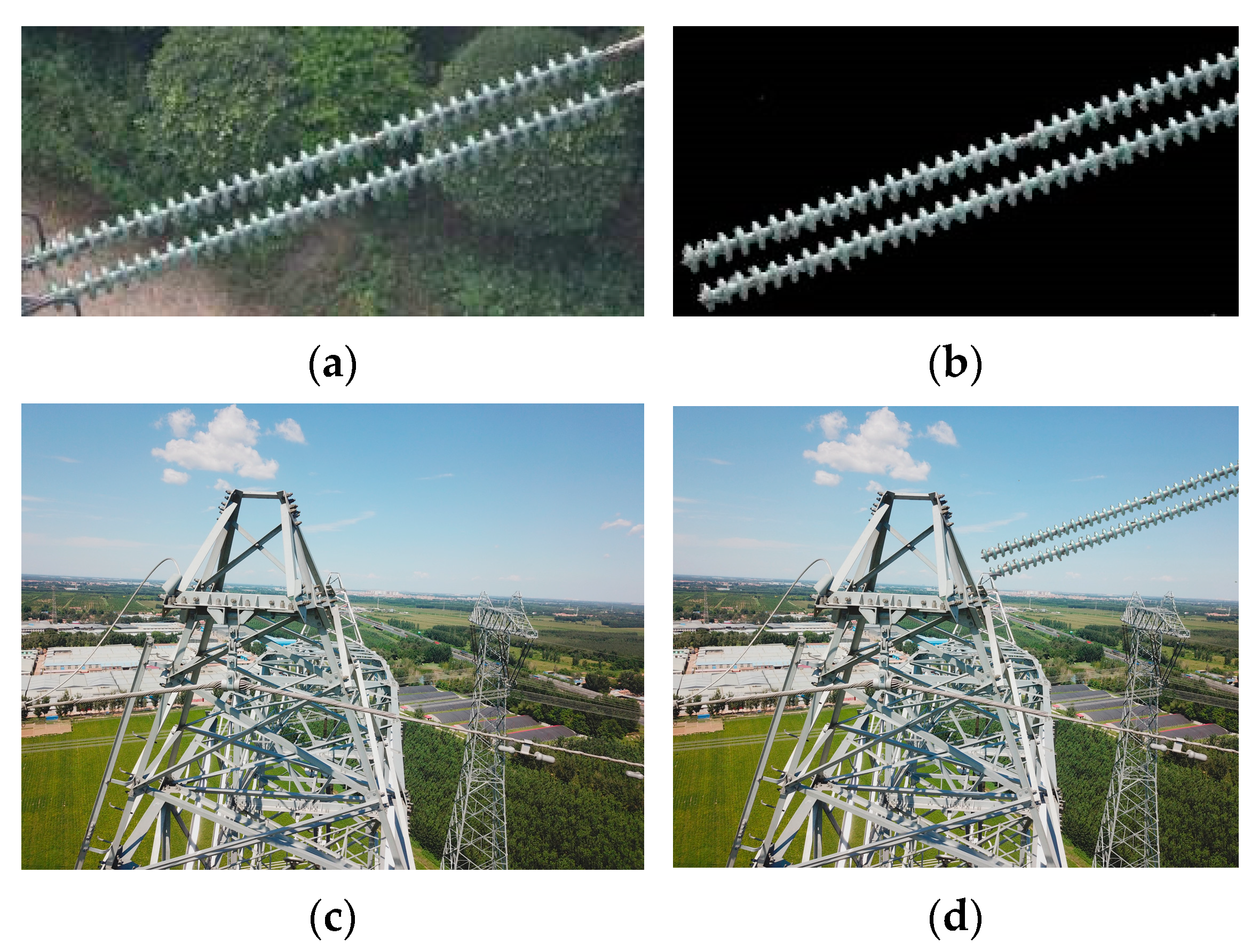
The images acquired by transmission line inspection are usually with different shooting angle, uneven illumination, and complex backgrounds. In order to obtain a more robust, stable, and generalizable deep learning model, the GraphCut segmentation algorithm was used to extract defective insulator targets, which were blended with the background image of practical power grid environment. The constructed defective insulator images based on this image blending method can not only expand the sample set, but also balance the sample numbers of normal insulators and defective insulators.
The GraphCut segmentation algorithm [31] uses the energy function E(x) to determine each pixel in the image is whether foreground or background. An image is defined as G = (X, Y), where X represents all pixel nodes in the image and Y represents the connection edge between nodes. For anyone node i∈X in the image, xi = 1 if i belongs to the foreground target; otherwise, xi = 0 if i belongs to the background. Thus, the image segmentation problem can be described as an extreme value solution of energy function. The energy function of image segmentation is defined as
where E1 is the energy consumed by defining the node i as the foreground or background; E2 is the energy cost of two adjacent and different pixel nodes, which depends on the color similarity of two pixels; and λ is the energy balance parameter and it is generally taken as λ = 50, which is a compromise between model-based classification and smooth-based classification. The calculation of energy E1 and E2 can refer to literature [32], and then the minimum value of E(x) is obtained by MaxFlow [33], so as to realize the segmentation of insulators in the image. Finally, the segmented insulator target was fused with the real and complex background image of the transmission line to form a virtual insulator defect image sample, as shown in Figure 1. This method can generate a large number of image samples containing real backgrounds and defective insulator targets, thereby avoiding the imbalance numbers between normal insulators and defective insulators, improving the robustness and generalization ability of the model.
2.2. Laplacian Sharpening
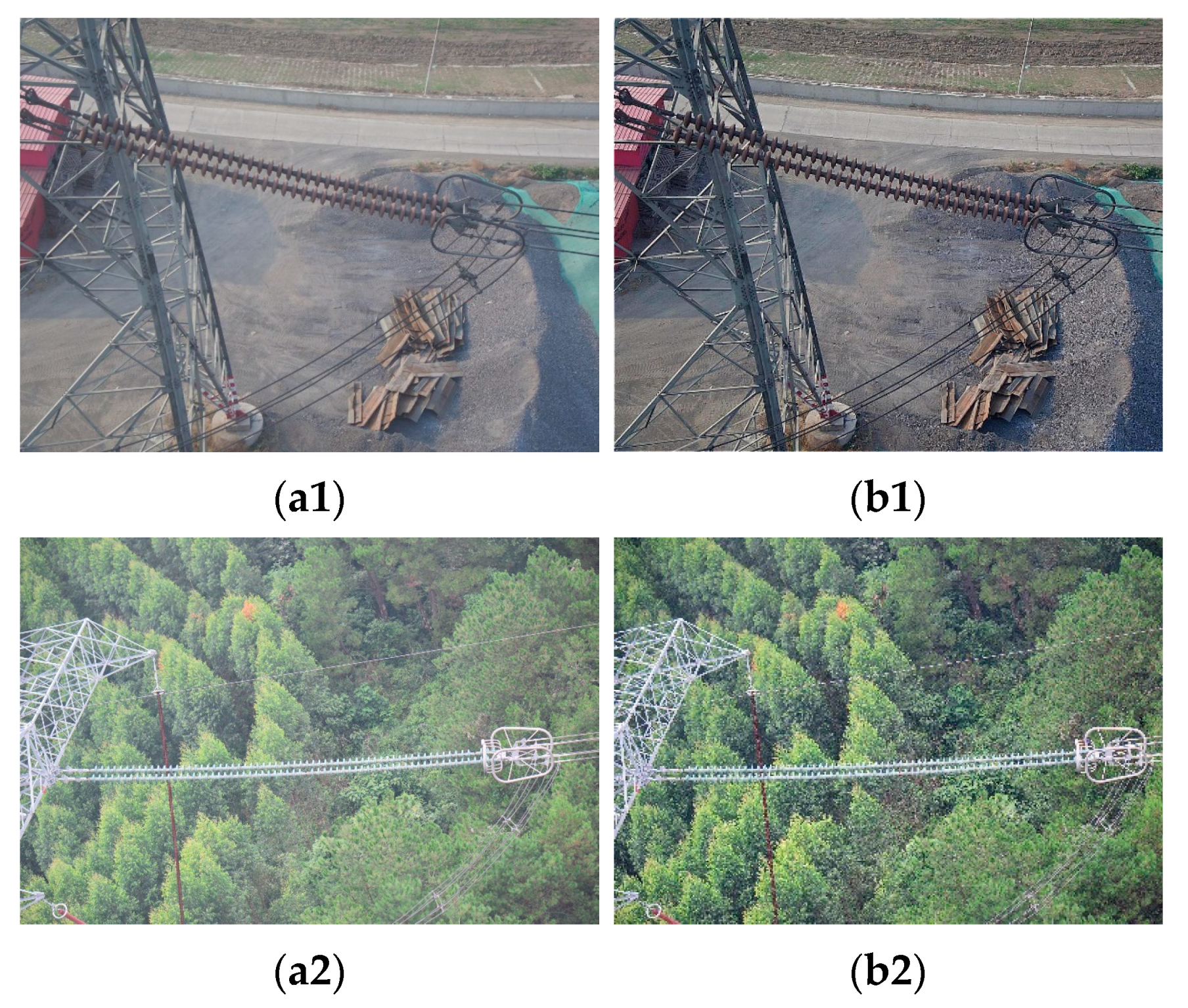
The color of insulator string is often too similar to the background and not easy to distinguish at the edge. In order to highlight the edge details of the target insulators in the image and improve the contrast, the Laplacian sharpening was used for image enhancement. For the binary insulator image f(x, y), the Laplace transform is
Then, the second-order partial differentials of the binary image f(x, y) in the direction of x and y are
Substituting the Equations (3) and (4) into Equation (2), the Laplace operator is
According to Equation (5), the sharpening filter is (0, 1, 0; 1, −4, 1; 0, 1, 0). Then, the Laplace image can be extracted by convoluting the original image with the original image. Furthermore, the original image and the Laplace image were superimposed according to Equation (6) to obtain the g(x,y) of the sharpened image. The comparison of images before and after Laplacian sharpening is shown in Figure 2 and no matter overall or locally, the sharpened image can effectively improve the contrast and reduce the influence of image blur and mist.
2.3. Transmission Line Insulator Image Dataset
The transmission line insulator image dataset used in this paper was partly derived from the China power line insulator dataset (CPLID) [14], which was already published on the Internet, including 600 normal insulator images and 248 defective insulator images. Another 216 images were collected from the UAV inspection results of high voltage transmission lines. Other images were generated by image augmentation method based on the GraphCut segmentation. The above samples together constitute the transmission line insulator image dataset, with a total of 2403 pictures.
The transmission line insulator image dataset needs to be annotated before training the object detection model. In this paper, the MRLabeler labeling tool was used to annotate the location and category of the insulator and its defect by a bounding box. Regardless of normal or defective insulators, their location and category were labeled as ‘insulator’. While, for defective insulators, the location and category of the defect were labeled as ‘defect’. This labeling method makes it possible to learn the spatial relationships between defects and insulators during model training. The annotation format is Pascal VOC [34], a common format in the field of computer vision, and the target location information can be obtained from the upper left vertex coordinates (xmin, ymax) and lower right vertex coordinates (xmax, ymin) of the bounding boxes.
3. Detection Model of Transmission Line Insulator Defects
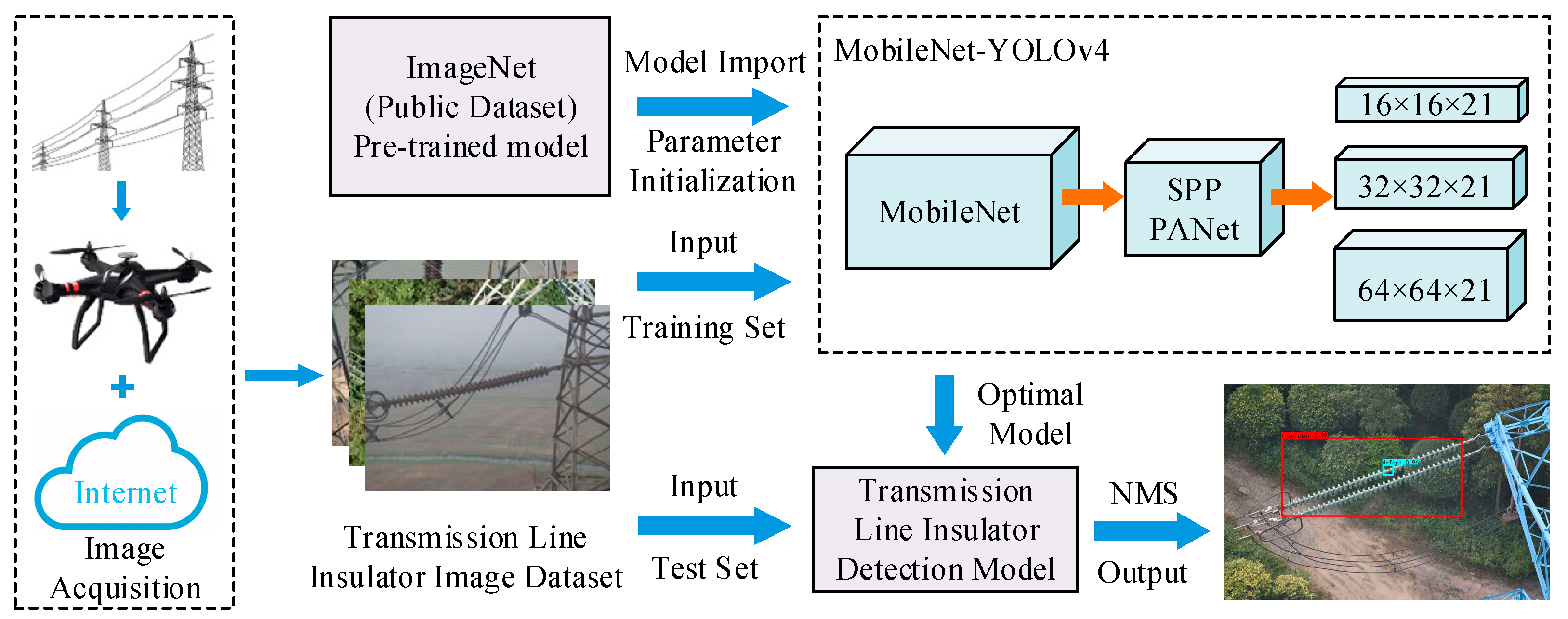
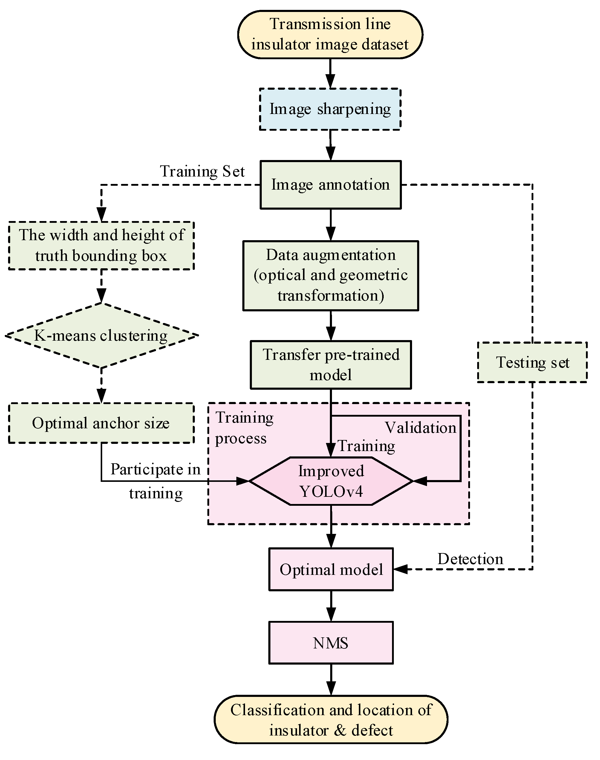
Aiming at the problems that the size of insulator defects is too small in the transmission line inspection images, some insulators are not significant in the real environment, the overlapping occlusion of insulators is serious and the speed of model detection is slow. An improved YOLOv4 algorithm model was proposed in this paper to realize fast and accurate detection of insulator defects during transmission line inspection, and the process of insulator defect detection is shown in Figure 3. The basic principles of the model are introduced as follows.
3.1. YOLOv4 Detection Algorithm
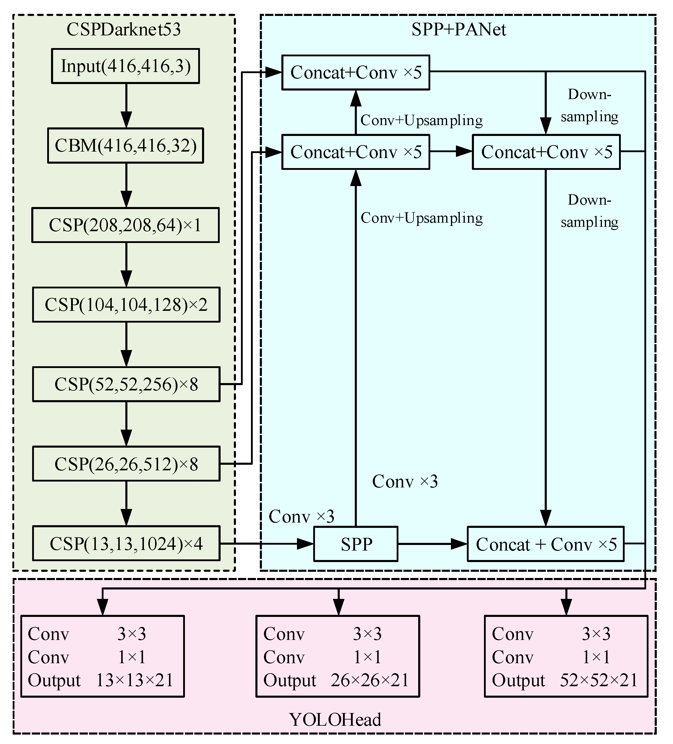
The main advantage of the series of YOLO (you only look once) algorithms is that the detection speed is fast, but the early versions of the YOLO algorithm are not accurate enough. However, YOLOv4 [35] introduced by Alexey in 2020 improves the detection performance of the model by introducing the advantages and tricks from other detection models, which is a mainstream detection algorithm in the field of object detection. There-fore, YOLOv4 has good detection accuracy and detection speed, and can be used as the basic detection network to realize the lightweight of the model, thus facilitating the deployment of the detection model. The structure of YOLOv4 is shown in Figure 4. It can be seen that YOLOv4 mainly includes feature extraction network (CSPDarknet53), feature pyramid (SPP and PANet) and prediction network (YOLOHead). The different modules of YOLOv4 and their functions are introduced below.
Firstly, the input images will be transmitted to the CBM module, which consists of convolution layer (Conv), batch normalization layer (BN), and activation function layer (Mish). Secondly, five CSP modules are used to extract features with three scales including 52 × 52, 26 × 26, 13 × 13. The features of different scales are fused through the spatial pyramid pooling (SPP) [36] and path aggregation network (PANet) [37]. Then, the classification and position of targets are predicted through the 3 × 3 and 1 × 1 convolutions. Finally, non-maximum suppression (NMS) [38] is used to eliminate redundant bounding boxes, thus obtaining the final predicted bounding box.
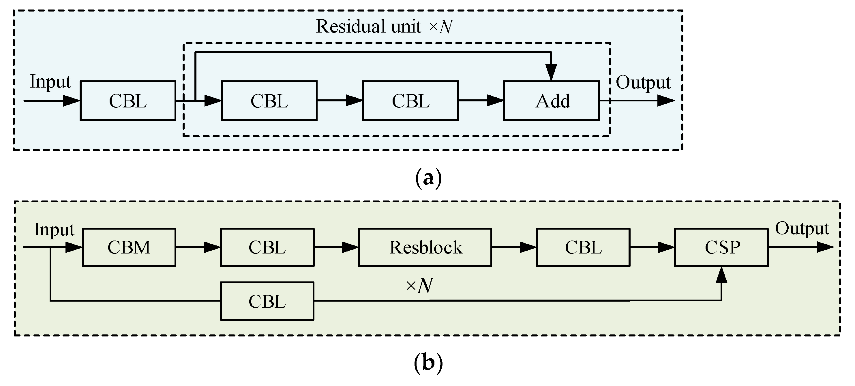
Among them, the CSPDarknet53 feature extraction network is an improved feature extractor based on Darknet53 feature extraction network in YOLOv3 and CSPNet [39], and the difference between CSPDarknet53 and Darknet53 is shown in Figure 5. The CSP module not only contains multiple resblocks, but also connects the input to the corresponding output through N resblocks by means of the cross stage partial connections. As for the value of N resblocks in the CSPDarknet53, it was set to five types of 1, 2, 8, 8, and 4, which has been shown to have good feature extraction ability and high detection precision. Moreover, in addition to improving the feature extractor, YOLOv4 also uses the SPP and PANet to enhance the representation capacity of features. The SPP concatenates feature maps after maxpooling with different pooling kernel sizes (1 × 1, 5 × 5, 9 × 9, 13 × 13) as output, which can increase the receptive field of feature extractor more effectively than the maxpooling with a single kernel size, and significantly separate important context features. Furthermore, the context features separated by SPP layer would be input into the PANet network, and the deep and shallow features are fused through convolution, upsampling, and down-sampling. Finally, YOLOHead uses repeatedly fused features to achieve target recognition and location.
3.2. Depthwise Separable Convolution
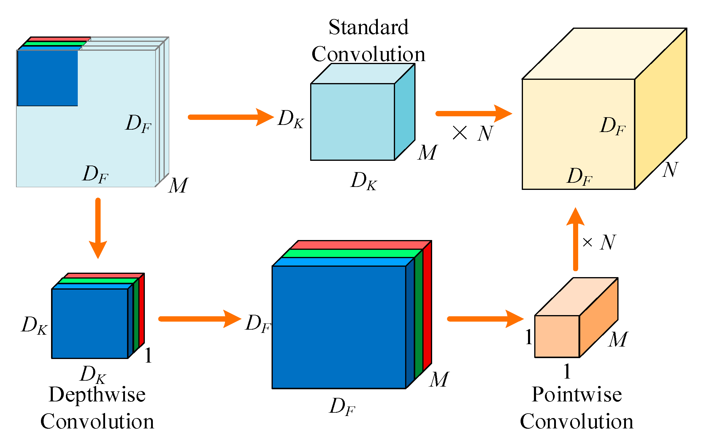
Depthwise separable convolution (DSC) is the core components of MobileNet [40]. It replaces the original 3 × 3 standard convolution with 3 × 3 depthwise convolution and 1 × 1 pointwise convolution. The principle of depthwise convolution is to use a single convolution kernel for each input channel to extract features, while 1 × 1 pointwise convolution is used for linear feature fusion of multiple outputs of depthwise convolution. DSC breaks the connection between the output channel and the convolution kernel, thus reducing the computational complexity of the model. Compared with standard convolution, the principle is shown in Figure 6.
Suppose the input image size is DF × DF × M, if the standard convolution is adopted, the parameter quantity is
where DK is the size of the convolution kernel, M is the number of input channels, and N is the number of output channels. If depthwise separable convolution is used, the parameter quantity of depthwise convolution and pointwise convolution is
where CDW and CPW are the corresponding parameter quantity of depthwise convolution and pointwise convolution. According to Equation (9), the parameter quantity of deep separable convolution is 1/N + 1/Dk2 of the standard convolution parameter quantity, and N≫ in the general model structure. The convolution kernel DK × DK commonly used in MobileNet is 3 × 3, so the parameter quantity of the DSC can be reduced to 1/8~1/9 of the standard convolution parameter quantity.
Since the practical deployment on mobile devices requires less parameter quantity and a high detection speed of the model, in MobileNet the number of channels in the model is multiplied by a hyperparameter, which is called width multiplier α. Then the parameter quantity of the convolution operation is
The default value of α in the standard MobileNet is 1.0, and the computation and parameter quantity of the model can be effectively reduced with a less α value. The values of α are usually set as 1.0, 0.75, 0.5, 0.25.
3.3. Improved YOLOv4 Insulator Defect Detection Model
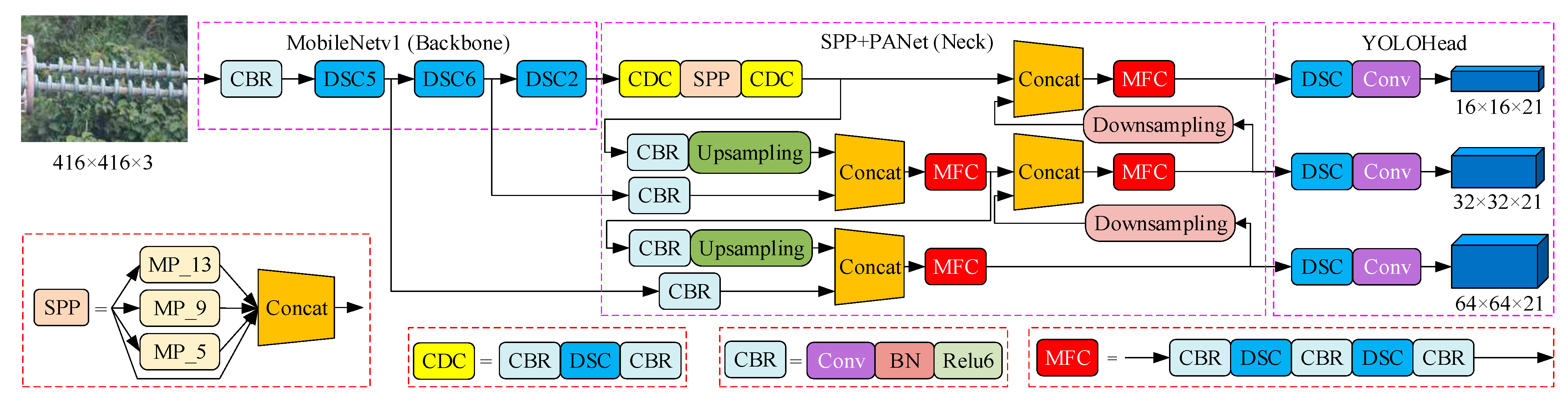
The model structure of improved YOLOv4 based on MobileNet is shown in Figure 7, where the number behind the DSC represents the amount of the DSC module. The CBR convolution module is similar to the CBM module in Figure 4, except that the activation layer is the ReLU6 activation function. The CDC module indicates that the input has been convolutional calculated for three times, including two convolution types CBR and DSC. The MFC module represents that the input has been convolutional calculated for five times, which also includes CBR and DSC. According to Figure 4 and Figure 7 the main improvement lies in the replacement of the feature extraction network and the improvement of the PANet based on DSC, which are described in detail as follows.
- Feature Extraction Network
The feature extraction network adopted by YOLOv4 is CSPDarknet53. By replacing the CSPDarknet53 with MobileNet, the input size required by the initial network is reshaped from 224 × 224 to 416 × 416. According to the convolution operation, the features after five DSC modules are extracted as feature 1, and the features after six DSC modules are extracted as feature 2, the features after two DSC modules are extracted as feature 3. The sizes of the three feature maps in the improved YOLOv4 model will be reshaped to 64 × 64, 32 × 32, and 16 × 16, while the sizes in YOLOv4 are 52 × 52, 26 × 26, and 13 × 13. Then the features 1, 2, and 3 are used for pooling and feature fusion of SPP and PANet. In addition, the Mish activation function in YOLOv4 is replaced by the ReLU6 activation function in MobileNet, the function expression is
- 2.
- DSC-SPP and DSC-PANet
It is found through tests that the total parameter quantity in YOLOv4 is about 64.43 million. If only the feature extraction network is replaced by the standard MobileNet with α = 1, the total parameter quantity in YOLOv4 is about 41 million and the number of parameters is not significantly reduced. The reason is that most of parameters in YOLOv4 are concentrated in the convolution operation of PANet. Therefore, in order to achieve a lighter detection model, the DSC was introduced into the SPP and PANet, which are improved as DSC-SPP and DSC-PANet. Firstly, the standard convolutions (Conv × 3), composed of three CBR, before and after SPP network are replaced with CDC module. In detail, the second CBR in Conv × 3 is replaced with DSC, as shown in Figure 7 and keeps the number of output channels unchanged. Then, the five standard convolution (Conv × 5) in the PANet network is improved as the MFC module, whose principle is to replace the second and fourth CBR with DSC. Finally, the standard convolution with the kernel 3 × 3 in YOLOHead is also replaced with DSC. Through the above three parts of improvements, the total parameters of the improved YOLOv4 detection model are about 12.75 million, which has been greatly reduced compared to the original YOLOv4 model.
3.4. Prediction Network
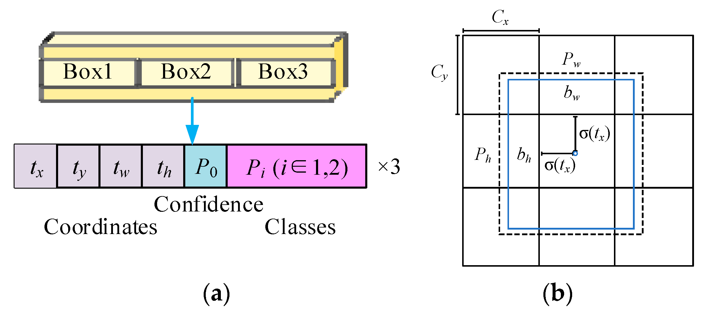
YOLO-Head uses multi-scale features obtained from the PANet structure to perform regression and classification prediction. In this part, PANet provides three feature maps, respectively, with sizes of 64 × 64 × 256, 32 × 32 × 512, and 16 × 16 × 1024 corresponding to shallow, middle, and deep prediction boxes. The scales of output feature maps in YOLO-Head are 64 × 64 × 21, 32 × 32 × 21, and 16 × 16 × 21, respectively. The third dimension is 21, which can be split into 3 × (2 + 5), as shown in Figure 8a; 2 represents the total number of categories in the transmission line insulator image dataset; 5 can be divided into 1 + 1 + 1 + 1 + 1, which respectively represent the x-axis offset, y-axis offset, height H, and width W of the prediction box, and confidence degree. When the prediction results are obtained, the prediction boxes can be drawn directly on the original picture.
The predicted output feature maps of three scales also need to be decoded, and the original picture will be decomposed into 64 × 64, 32 × 32, and 16 × 16 grids, just like the 3 × 3 grid in Figure 8b. The coordinates of each grid point plus its corresponding x-axis offset and y-axis offset are the coordinates of the center point of the prediction box, and then use the anchors and the prediction height H, width W to calculate the length and width of the prediction box. The calculation principle is shown in Equation (12). Finally, the prediction box on the original image can be obtained.
4. Case Study of Transmission Line Insulator Defect Detection
4.1. Simulation Environment and Evaluation Indexes
The transmission line insulator defect detection cases were completed in the software environment of Visual Studio Code 2016, Keras 2.1.5, TensorFlow 1.13.2, CUDA 10.0, cuDNN 7.4.1.5, and the hardware environment with GPU Nvidia GeForce GTX 1660 Super, 6 GB video memory.
In order to compare the performance of different models and algorithms, the precision (P), recall (R), average precision (AP), and mean average precision (mAP) are taken as indexes to evaluate model performance. The definitions of precision and recall are
where TP is the number of correctly positioned targets, TP + FP is the total number of positioned targets, and TP + FN is the total number of actual targets. The P–R curve can be plotted with the calculated P and R as ordinate and abscissa, while the area under the curve is AP, and the mean value of AP is mAP. For multi-class (N classes) object detection, the definitions of AP and mAP are
In addition, F1 score is also used to evaluate the performance of detection models, which represents the harmonic average of precision and recall and considers that precision and recall are equally important. The definition of F1 score is
In order to compare the detection speeds of different object detection models and reflect the real-time detection ability, this paper also introduces frames per second (FPS) as an evaluation index, which means the total number of images detected by the model in one second, that is, the time taken by the model to detect one image.
4.2. Implementation Process of Defect Detection
The implementation process is shown in Figure 9. The model is firstly pre-trained using ImageNet [41], a public image dataset. The pre-trained model is transferred to the transmission line insulator image dataset by the stage-wise training method, while the training process is divided into two stages. Moreover, before training the model, random combinations of geometric and optical transformations (including flip, scale, hue, etc.) will be used to augment the samples, thereby further increasing the robustness and generalization capabilities of the model. At the same time, three training techniques including Mosaic data augmentation, cosine annealing, and label smoothing were applied to improve the accuracy and generalization ability of the model.
In Figure 9, the optimal anchor size obtained based on the K-means clustering algorithm in the training set is (15,14 21,135 21,15; 39,18 81,21 107,36; 252,52 265,80 266,126), including the width and height of nine groups of anchors. The first three groups of anchors correspond to the 16 × 16 feature map, the middle three groups of anchors correspond to the 32 × 32 feature map, and the last three groups of anchors correspond to the 64 × 64 feature map, which are responsible for detecting targets of different sizes. The parameter settings during training and test are shown in Table 1.
4.3. Result Analysis
4.3.1. Detection Results with Different Proportion of Samples
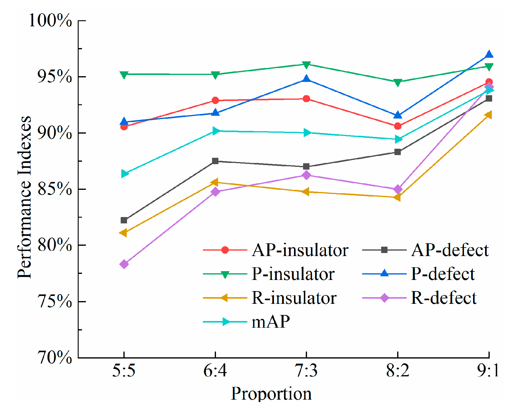
In order to analyze the influence under different proportion of insulator image samples on the detection accuracy, the proportions of the training set (including the validation set) and the test set were taken as 5:5, 6:4, 7:3, 8:2, and 9:1, and 10% of the samples in the training set were used as the validation set, as shown in Table 2. The performance indexes including P, R, AP, and mAP of the test results under different sample proportions are shown in Figure 10.
It can be seen from the Figure 10 that the values of P, R, AP, and mAP show upward trends with the increased proportion of training set to test set, and the proportion has a greater influence on insulator defect targets. When the proportion is 9:1, all the performance indexes have the maximum values, which are above 90%. The mAP value can reach 93.81%. Since the model has the highest detection accuracy, the proportion of 9:1 is used in the following analysis.
4.3.2. Detection Results with Different Width Multipliers
The influence of width multiplier α on detection accuracy was also analyzed. The test results with different values of α, namely, 0.25, 0.50, 0.75, and 1.0, were compared, and the performance indexes are shown in Figure 11.
It can be seen from Figure 11 that the P, R, and AP of defective insulators have upward trends with the increase in the width multiplier α. The R and AP of normal insulators also show upward trends, while the values of P decrease slightly, but they are all above 94% and the overall mAP also shows an upward trend. When α = 1.0, except for the value of P for normal insulators, the other performance indexes have the maximum values. According to the requirements in practical applications, the width multiplier α of the lightweight model can be adjusted flexibly to realize insulator defect detection with superior precision and high real-time performance.
4.3.3. Comparison with Different Detection Algorithms
In order to verify the effectiveness of the proposed method, four types of object detection models were also constructed, including Faster RCNN, SSD, YOLOv3, and YOLOv4. The transmission line insulator image dataset was also used for training and test of these object detection models. The detection results are shown in Table 3.
From the results in Table 3, the YOLOv4 detection algorithm achieves high-precision detection of insulators and its defects relying on its advantages of structure and training method. The mAP can reach 96.21%, which is higher than that of Faster RCNN, SSD, and YOLOv3, while the detection speed (FPS) of YOLOv4 is slow. The improved YOLOv4 model proposed in this paper can improve the detection speed to 53 pictures/s with the cost of 2.4% precision; that is, the time required to detect one image is about 18.87 ms, which is nearly 2.8 times the detection speed of YOLOv4. The detection accuracy is better than Faster RCNN, SSD, and YOLOv3. Moreover, the F1 scores of improved YOLOv4 are also superior to Faster RCNN, SSD, YOLOv3, and the F1 score of improved YOLOv4 in the category of the insulator defect is only 0.01 lower than YOLOv4. The above results verify that the proposed method can realize the defect detection of transmission line insulators with high precision and fast detection speed.
4.3.4. Influence of Image Sharpening Methods
In response to the problem of indistinct outline and low contrast caused by the similarity between the insulator target and the background, the Laplace image sharpening method was adopted to sharpen the transmission line insulator images, and compared with other three sharpening methods including sobel, prewitt, and laplacian of gaussian (log). The model detection results with different image sharpening methods are shown in Table 4.
From Table 4, it can be drawn that the application of image sharpening methods improves the detection ability of the model for insulator defects, with higher AP values compared to the non-sharpening condition. Among the above four sharpening algorithms, Laplace sharpening has the optimum indexes of insulator location and the highest AP and R of insulator defect detection, while the overall mAP can reach 97.26%, with the highest detection accuracy.
4.4. Generalization Ability and Robustness Verification
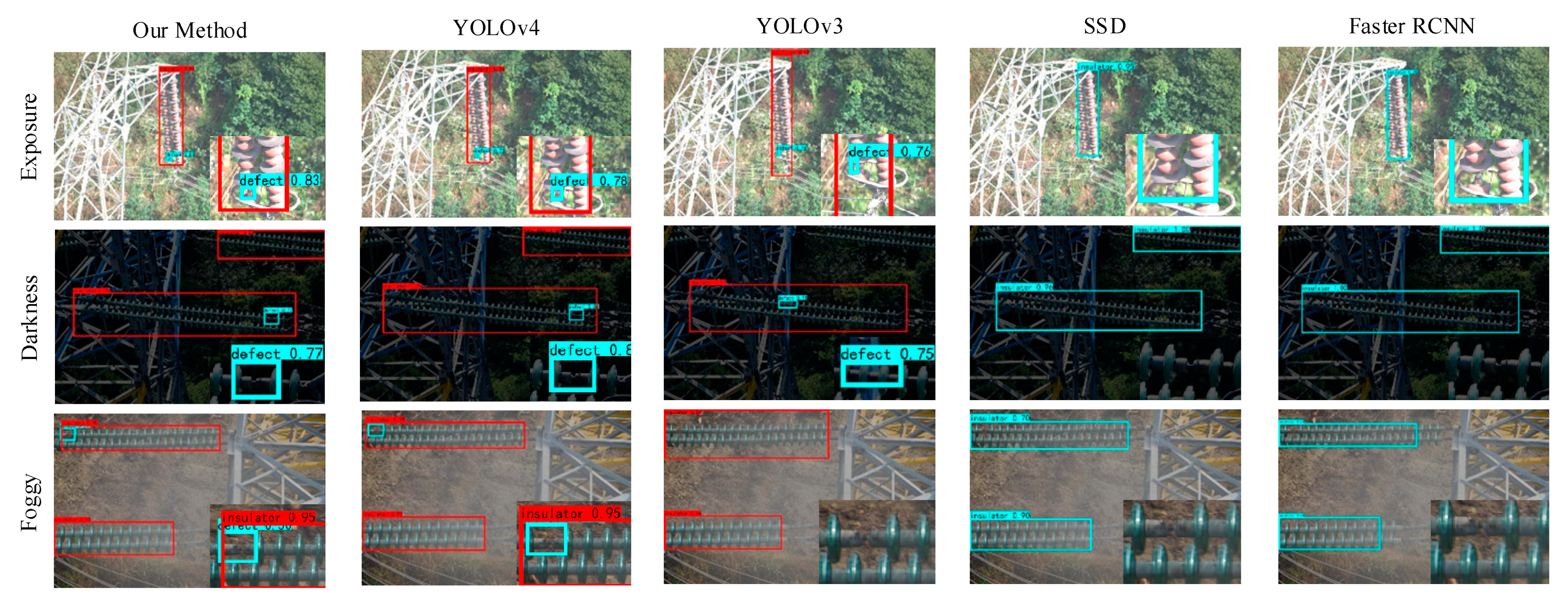
Due to the influence of time, weather, and angle during shooting, the UAV aerial images are prone to uneven illumination and blur. In consideration of the possible influence in practical applications, several preprocessing methods such as contrast and brightness adjustment and image atomization were adopted to simulate the conditions of extreme darkness, exposure, and foggy environment, so as to verify the generalization ability and robustness of the model.
The improved YOLOv4 model was used to detect images under the above three simulated conditions and the results were compared with Faster RCNN, SSD, YOLOv3, and YOLOv4 models, which are shown in Figure 12. The red bounding boxes in YOLOv3, YOLOv4, and the improved YOLOv4 represent the insulator, and the blue bounding boxes represent the defect class. However, the blue bounding boxes in SSD and Faster RCNN represent the insulator. According to the detection results, the YOLO models have superior accuracy in transmission line insulator location and defect detection, while the SSD and Faster RCNN have missed detections and poor detection effect on defect targets, which may be caused by small sizes of defect targets. Among YOLO models, YOLOv4 has the highest accuracy and can achieve accurate detection in the above three conditions. The improved YOLOv4 model, with lightweight feature extraction network MobileNet and optimized SPP and PANet network structures to reduce the number of parameters, can also achieve accurate detection in the three conditions. As for the detection speed (FPS), the proposed method increases the FPS to 53 pictures/s, which takes only 0.019 s to detect one image.
According to the above result analysis and model robustness verifications, it can be seen that the mAP and FPS of the improved YOLOv4 model can reach 93.81% and 53 pictures/s, respectively. In addition, Laplace sharpening can be applied to compensate for the loss of accuracy caused by lightweight model and improve the mAP to 97.26%. The case studies validate that the proposed method is able to realize accurate, fast, and automatic detection of transmission line insulator defects.
5. Conclusions
This paper constructs an improved YOLOv4 model based on lightweight CNN to detect the transmission line insulator defects in UAV aerial images. Case studies were carried out and different influence factors on the detection results were analyzed. The detection performance was also compared to other object detection models. The conclusions can be drawn as follows:
- The data augmentation method based on Graphcut segmentation is effective to expand the defective insulator images, which can avoid the problem of sample imbalance, improve the training effect and test accuracy, and therefore improve the generalization ability and robustness of the detection model.
- The lightweight YOLOv4 model improved by MobileNet, DSC-SPP, and DSC-PANet has good performance for detection of transmission line insulator defects, with a high detection accuracy and a fast detection speed. The mAP and FPS respectively reach 93.81% and 53 pictures/s, and the overall performance is better than that of Faster RCNN, SSD, YOLOv3, and YOLOv4 models.
- Laplace sharpening is able to compensate the detection accuracy of the lightweight YOLOv4 model, which increases the mAP to 97.26%, and its property is better than other sharpening methods including sobel, prewitt, and log. The proposed method is helpful for accurate detection of defective insulators on transmission lines, and applicable to meet the requirements of real-time detection in practical engineering.
Author Contributions
Conceptualization, Z.Q. and X.Z.; methodology, Z.Q. and X.Z.; software, W.Q.; validation, Z.Q. and X.Z.; formal analysis, D.S.; investigation, W.Q. and D.S.; resources, C.L.; data curation, Z.Q. and C.L.; writing—original draft preparation, Z.Q. and X.Z.; writing—review and editing, Z.Q., X.Z. and W.Q.; supervision, C.L.; project administration, Z.Q. All authors have read and agreed to the published version of the manuscript.
Funding
This work is supported by Jiangxi “Double Thousand Plan” Innovative Leading Talents Long-term Project, grant number jxsq2019101071, and Jiangxi Natural Science Foundation for Young Scholars, grant number 20192BAB216028.
Institutional Review Board Statement
Not applicable.
Informed Consent Statement
Not applicable.
Data Availability Statement
All data used in this research can be provided upon request.
Conflicts of Interest
The authors declare no conflict of interest.
References
- Park, K.C.; Motai, Y.; Yoon, J.R. Acoustic fault detection technique for high-power insulators. IEEE Trans. Ind. Electron. 2017, 64, 9699–9708. [Google Scholar] [CrossRef]
- Yang, Y.; Wang, L.; Wang, Y.; Mei, X. Insulator self-shattering detection: A deep convolutional neural network approach. Multimed. Tools Appl. 2019, 78, 10097–10112. [Google Scholar] [CrossRef]
- Yang, L.; Fan, J.; Liu, Y.; Li, E.; Peng, J.; Liang, Z. A review on state-of-the-art power line inspection techniques. IEEE Trans. Instrum. Meas. 2020, 69, 9350–9365. [Google Scholar] [CrossRef]
- Katrasnik, J.; Pernus, F.; Likar, B. A survey of mobile robots for distribution power line inspection. IEEE Trans. Power Deliv. 2009, 25, 485–493. [Google Scholar] [CrossRef]
- Nguyen, V.N.; Jenssen, R.; Roverso, D. Automatic autonomous vision-based power line inspection: A review of current status and the potential role of deep learning. Int. J. Electr. Power Energy Syst. 2018, 99, 107–120. [Google Scholar] [CrossRef] [Green Version]
- Matikainen, L.; Lehtomäki, M.; Ahokas, E.; Hyyppä, J.; Karjalainen, M.; Jaakkola, A.; Kukko, A.; Heinonen, T. Remote sensing methods for power line corridor surveys. ISPRS J. Photogramm. Remote Sens. 2016, 119, 10–31. [Google Scholar] [CrossRef] [Green Version]
- Wang, B.; Ma, F.; Ge, L.; Ma, H.; Wang, H.; Mohamed, M.A. Icing-EdgeNet: A pruning lightweight edge intelligent method of discriminative driving channel for ice thickness of transmission lines. IEEE Trans. Instrum. Meas. 2020, 70, 1–12. [Google Scholar] [CrossRef]
- Li, J.; Yan, D.; Luan, K.; Li, Z.; Liang, H. Deep learning-based bird’s nest detection on transmission lines using UAV imagery. Appl. Sci. 2020, 10, 6147. [Google Scholar] [CrossRef]
- Zhao, Z.; Qi, H.; Qi, Y.; Zhang, K.; Zhai, Y.; Zhao, W. Detection method based on automatic visual shape clustering for pin-missing defect in transmission lines. IEEE Trans. Instrum. Meas. 2020, 69, 6080–6091. [Google Scholar] [CrossRef] [Green Version]
- Zhang, W.; Liu, X.; Yuan, J.; Xu, L.; Sun, H.; Zhou, J.; Liu, X. RCNN-based foreign object detection for securing power transmission lines (RCNN4SPTL). Procedia Comput. Sci. 2019, 147, 331–337. [Google Scholar] [CrossRef]
- Hosseini, M.M.; Umunnakwe, A.; Parvania, M.; Tasdizen, T. Intelligent damage classification and estimation in power distribution poles using unmanned aerial vehicles and convolutional neural networks. IEEE Trans. Smart Grid 2020, 11, 3325–3333. [Google Scholar] [CrossRef]
- Davari, N.; Akbarizadeh, G.; Mashhour, E. Intelligent diagnosis of incipient fault in power distribution lines based on corona detection in UV-visible videos. IEEE Trans. Power Deliv. 2020, 36, 3640–3648. [Google Scholar] [CrossRef]
- Rong, S.; He, L.; Du, L.; Li, Z.; Yu, S. Intelligent detection of vegetation encroachment of power lines with advanced stereovision. IEEE Trans. Power Deliv. 2020, 36, 3477–3485. [Google Scholar] [CrossRef]
- Tao, X.; Zhang, D.; Wang, Z.; Liu, X.; Zhang, H.; Xu, D. Detection of power line insulator defects using aerial images analyzed with convolutional neural networks. IEEE Trans. Syst. Man Cybern. Syst. 2018, 50, 1486–1498. [Google Scholar] [CrossRef]
- Ling, Z.; Zhang, D.; Qiu, R.C.; Jin, Z.; Zhang, Y.; He, X.; Liu, H. An accurate and real-time method of self-blast glass insulator location based on faster R-CNN and U-net with aerial images. CSEE J. Power Energy Syst. 2019, 5, 474–482. [Google Scholar] [CrossRef]
- Liu, X.; Miao, X.; Jiang, H.; Chen, J. Box-Point Detector: A diagnosis method for insulator faults in power lines using aerial images and convolutional neural networks. IEEE Trans. Power Deliv. 2021, 36, 3765–3773. [Google Scholar] [CrossRef]
- Sadykova, D.; Pernebayeva, D.; Bagheri, M.; James, A. IN-YOLO: Real-time detection of outdoor high voltage insulators using UAV imaging. IEEE Trans. Power Deliv. 2019, 35, 1599–1601. [Google Scholar] [CrossRef]
- Wang, B.; Dong, M.; Ren, M.; Wu, Z.; Guo, C.; Zhuang, T.; Pischler, O.; Xie, J. Automatic fault diagnosis of infrared insulator images based on image instance segmentation and temperature analysis. IEEE Trans. Instrum. Meas. 2020, 69, 5345–5355. [Google Scholar] [CrossRef]
- Han, J.; Yang, Z.; Zhang, Q.; Chen, C.; Li, H.; Lai, S.; Hu, G.; Xu, C.; Xu, H.; Wang, D.; et al. A method of insulator faults detection in aerial images for high-voltage transmission lines inspection. Appli. Sci. 2019, 9, 2009. [Google Scholar] [CrossRef] [Green Version]
- Wen, Q.; Luo, Z.; Chen, R.; Yang, Y.; Li, G. Deep learning approaches on defect detection in high resolution aerial images of insulators. Sensors 2021, 21, 1033. [Google Scholar] [CrossRef]
- Liu, X.; Li, Y.; Shuang, F.; Gao, F.; Zhou, X.; Chen, X. ISSD: Improved SSD for insulator and spacer online detection based on UAV system. Sensors 2020, 20, 6961. [Google Scholar] [CrossRef] [PubMed]
- Yu, J.; Zhang, W. Face mask wearing detection algorithm based on improved YOLO-v4. Sensors 2021, 21, 3263. [Google Scholar] [CrossRef] [PubMed]
- Roy, A.M.; Bose, R.; Bhaduri, J. A fast accurate fine-grain object detection model based on YOLOv4 deep neural network. arXiv 2021, arXiv:2111.00298. [Google Scholar] [CrossRef]
- Zha, M.; Qian, W.; Yi, W.; Hua, J. A lightweight YOLOv4-Based forestry pest detection method using coordinate attention and feature fusion. Entropy 2021, 23, 1587. [Google Scholar] [CrossRef]
- Yang, Q.; Zhang, Z.; Yan, L.; Wang, W.; Zhang, Y.; Zhang, C. Lightweight bird’s nest location recognition method based on YOLOv4-tiny. In Proceedings of the 2021 IEEE International Conference on Electrical Engineering and Mechatronics Technology (ICEEMT), Qingdao, China, 2–4 July 2021. [Google Scholar] [CrossRef]
- Qiu, Z.; Zhu, X.; Liao, C.; Shi, D.; Kuang, Y.; Li, Y.; Zhang, Y. Detection of bird species related to transmission line faults based on lightweight convolutional neural network. IET Gener. Transm. Distrib. 2021. [Google Scholar] [CrossRef]
- Chollet, F. Xception: Deep learning with depthwise separable convolutions. In Proceedings of the 2017 IEEE Conference on Computer Vision and Pattern Recognition (CVPR), Honolulu, HI, USA, 21–26 July 2017. [Google Scholar] [CrossRef] [Green Version]
- Krizhevsky, A.; Sutskever, I.; Hinton, G. ImageNet classification with deep convolutional neural networks. Adv. Neural Inf. Process. Syst. 2012, 25, 84–90. [Google Scholar] [CrossRef]
- Lin, M.; Chen, Q.; Yan, S. Network in Network. arXiv 2013, arXiv:1312.4400. [Google Scholar]
- Zhang, X.; Zhou, X.; Lin, M.; Sun, J. ShuffleNet: An extremely efficient convolutional neural network for mobile devices. arXiv 2017, arXiv:1707.01083. [Google Scholar]
- Boykov, Y.Y.; Jolly, M. Interactive graph cuts for optimal boundary & region segmentation of objects in n-d images. In Proceedings of the 8th International Conference on Computer Vision (ICCV), Vancouver, BC, Canada, 7–14 July 2001. [Google Scholar] [CrossRef]
- Wang, Y. An enhanced scheme for interactive image segmentation. J. Univ. Sci. Technol. China 2010, 40, 129–132. [Google Scholar] [CrossRef]
- Boykov, Y.; Kolmogorov, V. An experimental comparison of min-cut/max-flow algorithms for energy minimization in vision. IEEE Trans. Pattern Anal. Mach. Intell. 2004, 26, 1124–1137. [Google Scholar] [CrossRef] [Green Version]
- Everingham, M.; Van Gool, L.; Williams, C.K.I.; Winn, J.; Zisserman, A. The pascal visual object classes (voc) challenge. Int. J. Comput. Vis. 2010, 88, 303–338. [Google Scholar] [CrossRef] [Green Version]
- Bochkovskiy, A.; Wang, C.Y.; Liao, H.Y.M. YOLOv4: Optimal speed and accuracy of object detection. arXiv 2020, arXiv:2004.10934. [Google Scholar]
- He, K.; Zhang, X.; Ren, S.; Sun, J. Spatial pyramid pooling in deep convolutional networks for visual recognition. IEEE Trans. Pattern Anal. Mach. Intell. 2015, 37, 1904–1916. [Google Scholar] [CrossRef] [PubMed] [Green Version]
- Liu, S.; Qi, L.; Qin, H.; Shi, J.; Jia, J. Path aggregation network for instance segmentation. In Proceedings of the 2018 IEEE/CVF Conference on Computer Vision and Pattern Recognition, Salt Lake City, UT, USA, 18–23 June 2018. [Google Scholar] [CrossRef] [Green Version]
- Neubeck, A.; Van Gool, L. Efficient non-maximum suppression. In Proceedings of the 18th International Conference on Pattern Recognition (ICPR), Hong Kong, China, 20–24 August 2006. [Google Scholar] [CrossRef]
- Wang, C.Y.; Liao, H.Y.M.; Wu, Y.H.; Chen, P.-Y.; Hsieh, J.W.; Yeh, I.H. CSPNet: A new backbone that can enhance learning capability of CNN. In Proceedings of the 2020 IEEE/CVF Conference on Computer Vision and Pattern Recognition Workshops (CVPRW), Seattle, WA, USA, 14–19 June 2020. [Google Scholar] [CrossRef]
- Howard, A.G.; Zhu, M.; Chen, B.; Kalenichenko, D.; Wang, W.; Weyand, T.; Andreetto, M.; Adam, H. Mobilenets: Efficient convolutional neural networks for mobile vision applications. arXiv 2017, arXiv:1704.04861. [Google Scholar]
- Deng, J.; Dong, W.; Socher, R.; Li, L.J.; Li, K.; Li, F.F. ImageNet: A large-scale hierarchical image database. In Proceedings of the 2009 IEEE Conference on Computer Vision and Pattern Recognition (CVPR), Miami, FL, USA, 20–25 June 2009. [Google Scholar] [CrossRef] [Green Version]
Figure 1.
Schematic diagrams of image augmentation: (a) Original image, (b) Segmentation image, (c) Background image, (d) Composite image.
Figure 1.
Schematic diagrams of image augmentation: (a) Original image, (b) Segmentation image, (c) Background image, (d) Composite image.

Figure 2.
Comparison of images before and after Laplacian sharpening: (a1) Original image, (a2) Original image, (b1) Sharpened image, (b2) Sharpened image.
Figure 2.
Comparison of images before and after Laplacian sharpening: (a1) Original image, (a2) Original image, (b1) Sharpened image, (b2) Sharpened image.

Figure 3.
Detection process of insulators on transmission line.

Figure 4.
Structure of YOLOv4 algorithm.

Figure 5.
Difference between CSPDarknet53 and Darknet53 feature extraction: (a) Resblock, (b) Cross stage partial network.
Figure 5.
Difference between CSPDarknet53 and Darknet53 feature extraction: (a) Resblock, (b) Cross stage partial network.

Figure 6.
Principle of depthwise separable convolution.

Figure 7.
Structure of improved YOLOV4 algorithm.

Figure 8.
Multi-scale prediction principle: (a) The third-dimension calculation principle of output feature maps in YOLO-Head, (b) Prediction box regression.
Figure 8.
Multi-scale prediction principle: (a) The third-dimension calculation principle of output feature maps in YOLO-Head, (b) Prediction box regression.

Figure 9.
Model training and test process.

Figure 10.
Performance indexes under different proportions of sample.

Figure 11.
Performance indexes under different width multipliers.

Figure 12.
Detection results of different models under simulated environment.


Table 1.
Simulation parameter setting.
| Parameters | First Stage | Second Stage |
|---|---|---|
| Batchsize | 8 | 2 |
| Initial learning rate | 1 × 10⁻³ | 1 × 10⁻⁴ |
| Training epochs | 50 | 50 |
| IoU threshold | 0.5 | |
| NMS threshold | 0.3 | |
| Label smoothing value | 0.01 | |
| Minimum learning rate of cosine annealing | 1 × 10⁻⁶ | |
Table 2.
Number of samples in different proportions.
| Proportion | Training Set | Validation Set | Test Set |
|---|---|---|---|
| 5:5 | 1081 | 120 | 1202 |
| 6:4 | 1297 | 144 | 962 |
| 7:3 | 1514 | 168 | 721 |
| 8:2 | 1730 | 192 | 481 |
| 9:1 | 1946 | 216 | 241 |
Table 3.
Performance indexes of different detection models.
| Method | AP (%) | mAP (%) | F1 Score | FPS (pictures/s) | ||
|---|---|---|---|---|---|---|
| Insulator | Defect | Insulator | Defect | |||
| Faster RCNN | 87.27 | 92.54 | 79.91 | 0.79 | 0.92 | 1 |
| SSD | 93.81 | 75.03 | 84.42 | 0.81 | 0.72 | 28 |
| YOLOv3 | 89.00 | 87.33 | 88.16 | 0.88 | 0.89 | 24 |
| YOLOv4 | 96.14 | 96.43 | 96.21 | 0.96 | 0.95 | 19 |
| Improved YOLOv4 | 94.53 | 93.09 | 93.81 | 0.96 | 0.94 | 53 |
Table 4.
Performance indexes of detection model with different sharpening methods.
| Sharpening Method | Insulator Location | Insulator Defect Location | mAP (%) | ||||
|---|---|---|---|---|---|---|---|
| AP (%) | P (%) | R (%) | AP (%) | P (%) | R (%) | ||
| Non-sharpening | 94.53 | 95.96 | 91.63 | 93.09 | 96.97 | 94.12 | 93.81 |
| prewitt | 94.04 | 93.91 | 89.27 | 93.56 | 93.94 | 91.18 | 93.80 |
| sobel | 94.76 | 93.42 | 91.42 | 95.57 | 98.44 | 92.65 | 95.17 |
| log | 94.32 | 95.22 | 89.70 | 93.62 | 96.97 | 94.12 | 93.97 |
| laplacian | 96.15 | 96.69 | 93.99 | 98.40 | 95.59 | 95.59 | 97.26 |
Publisher’s Note: MDPI stays neutral with regard to jurisdictional claims in published maps and institutional affiliations. |
© 2022 by the authors. Licensee MDPI, Basel, Switzerland. This article is an open access article distributed under the terms and conditions of the Creative Commons Attribution (CC BY) license (https://creativecommons.org/licenses/by/4.0/).
Share and Cite
MDPI and ACS Style
Qiu, Z.; Zhu, X.; Liao, C.; Shi, D.; Qu, W. Detection of Transmission Line Insulator Defects Based on an Improved Lightweight YOLOv4 Model. Appl. Sci. 2022, 12, 1207. https://0-doi-org.brum.beds.ac.uk/10.3390/app12031207
AMA Style
Qiu Z, Zhu X, Liao C, Shi D, Qu W. Detection of Transmission Line Insulator Defects Based on an Improved Lightweight YOLOv4 Model. Applied Sciences. 2022; 12(3):1207. https://0-doi-org.brum.beds.ac.uk/10.3390/app12031207
Chicago/Turabian StyleQiu, Zhibin, Xuan Zhu, Caibo Liao, Dazhai Shi, and Wenqian Qu. 2022. "Detection of Transmission Line Insulator Defects Based on an Improved Lightweight YOLOv4 Model" Applied Sciences 12, no. 3: 1207. https://0-doi-org.brum.beds.ac.uk/10.3390/app12031207
Note that from the first issue of 2016, this journal uses article numbers instead of page numbers. See further details here.