Phase Mask Design Based on an Improved Particle Swarm Optimization Algorithm for Depth of Field Extension

Abstract

Phase mask optimization is one of the critical steps in designing a wavefront coding system to extend the depth of field (DoF). As a classical phase mask, a cubic phase mask was taken as an example. An improved particle swarm optimization (PSO) algorithm was applied to calculate the parameters of the cubic phase mask by introducing the modulation transfer function as the optimization criterion and a threshold as a constraint. The quality of the subsequent image restoration is guaranteed on the premise of the extended DoF. Finally, the improved PSO was proved to be faster, more efficient, and more accurate compared to the simulated annealing algorithm and the traditional PSO. The experimental results verify that the cubic phase mask optimized by the improved PSO can achieve DoF extension in the wavefront coding system. The improved PSO can also be applied to other phase masks of wavefront coding systems.

1. Introduction

Wavefront coding technology [1] has been proposed to extend the depth of field (DoF) without sacrificing resolution or luminous flux. This technology has been widely used in various optical systems, such as miniature optical endoscopes [2], microscopes [3], and conformal domes [4].

The phase mask plays a key role in the image quality of wavefront coding systems. Many optimization algorithms were applied to obtain an optimal phase mask, such as simulated annealing (SA) [5] and genetic algorithm (GA) [6]. These algorithms have achieved good results in DoF extension. However, the optimal solution and calculation time of SA are related to the cooling rate, number of temperature iterations, and temperature range. These parameter settings are very complicated, and it takes many attempts to obtain the right value. Otherwise, it is easy to fall into the local optimal solution. GA requires sufficient mutations. Otherwise, GA will fall into a local optimal solution. However, sufficient mutations will prolong the optimization time.

People constantly pursue a fast, simple optimization algorithm that does not easily fall into the local optimal solution. Therefore, an improved particle swarm optimization (PSO) is proposed here as an optimization algorithm for optimizing phase masks in the design of wavefront coding systems. Based on PSO [7,8], we cancel the velocity range in PSO and introduce the restriction conditions, which not only restrict the optimization range of the phase mask parameter but also guarantee the quality of image recovery in the later stage. The improved PSO is simple to use, and only the number of iterations and the population of particles need to be set. The improved PSO can effectively jump out of the local optimal solution while guaranteeing the convergence speed and improving the optimization efficiency of the optical design process.

This paper is organized as follows. Section 2 provides the theoretical analysis of the wavefront coding technology, PSO, and phase mask parameter optimization based on improved PSO. Section 3 shows the simulation results and analyzes the performance of the improved PSO based on the simulation results, as well as a comparison with SA and traditional PSO. Section 4 shows the experimental results, which verify that the cubic phase mask optimized by the improved PSO can achieve DoF extension in the wavefront coding system. The conclusions are given in Section 5.

2. Methods

2.1. Theoretical Analysis of Wavefront Coding Systems

The DoF in object space corresponds to the depth of focus in image space. Consequently, a wavefront coding system that extends DoF in the object space is insensitive to the defocus in the image space. A cubic phase mask is a classic example applied in wavefront coding systems to extend the DoF. The one-dimensional cubic phase mask $f(x)$ is analyzed as an example for simplicity, which can be described as

$$f(x)=\alpha x^3,$$

(1)

where $x$, in the range of −1 to 1, is the coordinate of the phase mask and $\alpha$ is the cubic parameter of the phase mask. The pupil function, which ignores all optical aberrations but defocus, can be described as

$$p(x)=\exp [\mathrm{j}(f(x)+\varphi x^2)]$$

(2)

where $\varphi$ is the defocus aberration and $\mathrm{j}$ is the imaginary unit. The modulation transfer function (MTF), an image quality evaluation method, is used to evaluate the defocus insensitivity [9] of wavefront coding systems. MTF curves with different defocus aberrations will be coincident if the wavefront coding system is ideally defocus-insensitive. Consequently, the coincidence of MTF curves with different defocus aberrations is used as a merit function to evaluate the defocus insensitivity of the system.

$$s(\alpha )=\min {\displaystyle \iint {[MTF(\alpha ,u,\varphi )-MTF(\alpha ,u,{\varphi }_0)]}^{2}dud\varphi }$$

(3)

where $u$ is the spatial frequency and ${\varphi }_0$ is zero. However, wavefront coding systems suffer from a trade-off between defocus insensitivity and imaging quality [10]. To ensure imaging quality, the system should satisfy

$$t={\displaystyle \iint MTF(\alpha ,u,{\varphi }_0)dud\varphi \ge \mathrm{T}}$$

(4)

where the threshold $\mathrm{T}$ is 0.15 in this study [11].

2.2. Theoretical Analysis of PSO

Particle swarm optimization (PSO) [7,8] was proposed as a nonlinear optimization algorithm. With the rapid development of artificial intelligence and deep learning, PSO has a wide range of applications in many fields, such as the design of semiconductor lasers [12], intelligence-bearing fault diagnosis [13], and water quality monitoring [14].

PSO was applied to optimize the cubic phase mask of the wavefront coding system in this study. In this article, PSO is based on the standard “GBEST” version, which is the original form of PSO. The population of particles $D$ is the sum of particles. The parameter of cubic phase mask parameter in Equation (1) is denoted as ${\alpha }_d$, representing the position of the $d$th particle in the particles. Then, the position of the current particles can be denoted as an array

$$A=[{\alpha }_1,{\alpha }_2,{\alpha }_3,\dots ,{\alpha }_d,\dots ,{\alpha }_D]$$

Array $A$ is updated with each iteration. $I$ denotes the number of iterations in PSO. ${\alpha }^{\mathrm{global}}$ is the best location obtained so far by any particle in the population.

The fitness $s({\alpha }_d)$, the distance between the desired solution and the $d$th particle, is the coincidence consistency of the MTF curves in Equation (3). Ideally, $s({\alpha }_d)$ is equal to zero when the $d$th particle is the desired solution. Equation (4) is the constraint on the solution space. The fitness of the current particles can be denoted as array

$$S=[s({\alpha }_1),s({\alpha }_2),s({\alpha }_3),\dots ,s({\alpha }_d),\dots ,s({\alpha }_D)].$$

Velocity is an important parameter of PSO. $v_d$ is described as the $d$th particle velocity. The velocity represents the particle’s ability to explore the solution space. The velocity of the current particles can be denoted as array

$$V=[v_1,v_2,v_3,\dots ,v_d,\dots ,v_D].$$

The local optimal solution ${\alpha }_d^{\mathrm{local}}$ is the best location of the $d$th particle so far. The local optimal solution of the current particles can be denoted as the array

$$A^{\mathrm{local}}=[{\alpha }_1^{\mathrm{local}},{\alpha }_2^{\mathrm{local}},{\alpha }_3^{\mathrm{local}},\dots ,{\alpha }_d^{\mathrm{local}},\dots ,{\alpha }_D^{\mathrm{local}}].$$

In a similar way, the local optimal fitness of the current particles can be denoted as the array

$$S^{\mathrm{local}}=[s({\alpha }_1^{\mathrm{local}}),s({\alpha }_2^{\mathrm{local}}),s({\alpha }_3^{\mathrm{local}}),\dots ,s({\alpha }_d^{\mathrm{local}}),\dots ,s({\alpha }_D^{\mathrm{local}})].$$

The global optimal fitness is $s({\alpha }^{\mathrm{global}})$.

The locations and velocities are related to the experience, which is determined by the locations and velocities of all particles before their last move. They are updated after each iteration by these formulas [7,15]:

$$v_d=v_d+c_1·\mathrm{r}\mathrm{a}\mathrm{n}\mathrm{d}·({\alpha }_d^{\mathrm{local}}-{\alpha }_d)+c_2·\mathrm{r}\mathrm{a}\mathrm{n}\mathrm{d}·({\alpha }^{\mathrm{global}}-{\alpha }_d)$$

(5)

$${\alpha }_d={\alpha }_d^{\mathrm{local}}+v_d$$

(6)

where $\mathrm{rand}$ is a function of generating a random number between 0 and 1, setting the acceleration constants $c_1=2$ and $c_2=2$ [7,15].

2.3. Phase Mask Design Based on Improved Particle Swarm Optimization

If the range of velocity is too high, particles might fly past good solutions. If the value range of velocity is too small, particles may not explore sufficiently beyond locally good regions [15]. In brief, an inappropriate range of velocity is the factor that causes PSO to fall into a locally optimal solution. It is necessary to repeatedly test different velocity ranges to obtain the ideal optimal solution, which will greatly reduce the optimization efficiency of the algorithm.

In order to improve the optimization efficiency of the algorithm, this paper cancels the setting of the velocity range in PSO and introduces the threshold $\mathrm{T}$ of Equation (4).

The cubic phase mask parameter is limited by the threshold $\mathrm{T}$ in the optimization process. This measure can effectively prevent PSO from falling into the local optimal solution and ensure the quality of image restoration.

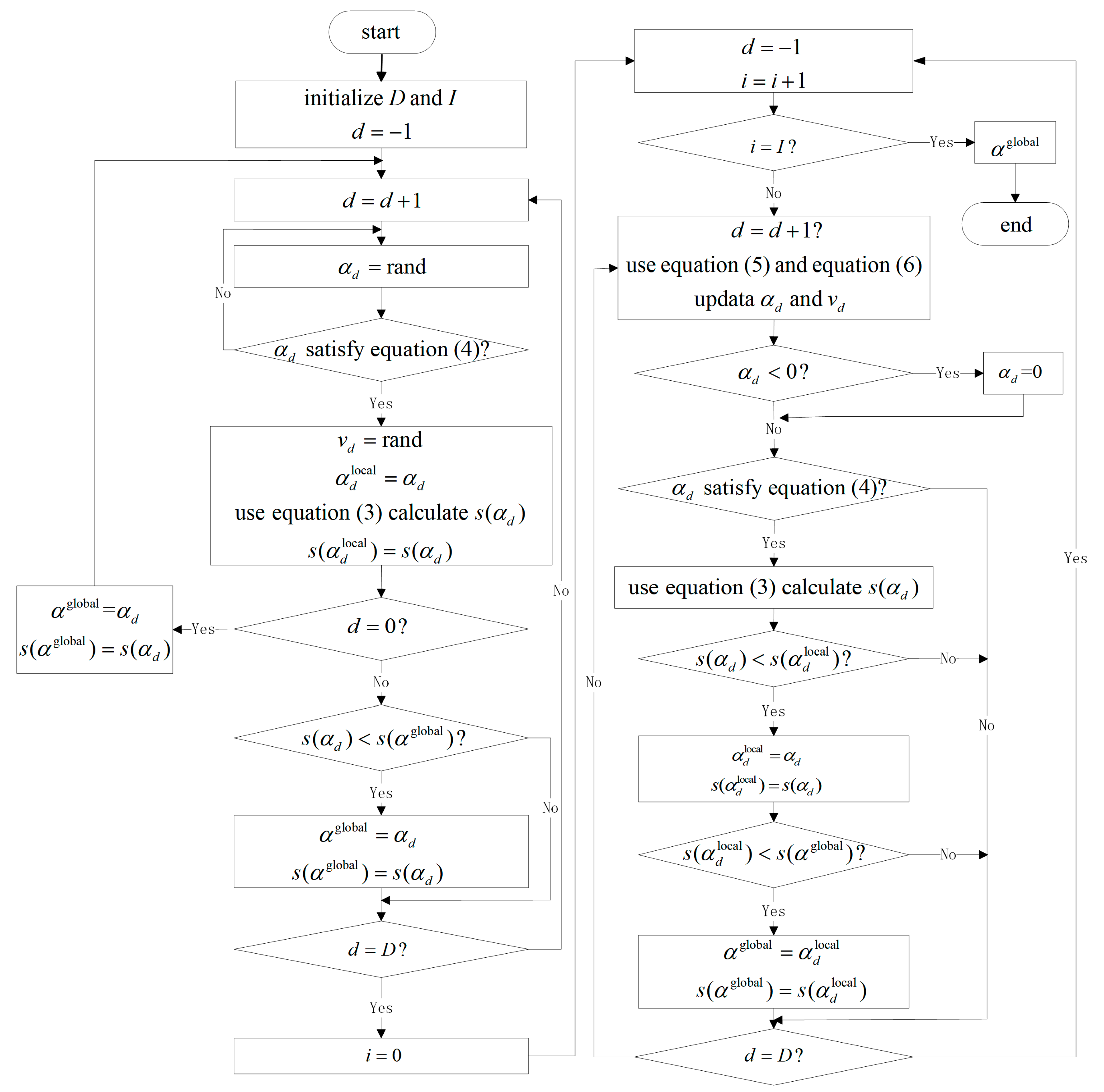
Combined with the characteristics of PSO and the cubic phase mask optimization problem, the phase mask optimization algorithm flow based on improved PSO is shown in Figure 1.

As shown in Figure 1, the specific process of the algorithm is as follows:

Assign the population of particles $D$ and the number of iterations $I$.

Initialize the initial position $A$ of particles and the corresponding fitness $S$. The initial ${\alpha }_d$ is assigned to a random number, and the initial ${\alpha }_d$ must satisfy Equation (4). Otherwise, the initial ${\alpha }_d$ needs to be reinitialized until it satisfies Equation (4). $s({\alpha }_d)$, the fitness of ${\alpha }_d$, is computed by Equation (3).

Initialize the initial velocity $V$ of particles. The initial $v_d$ is assigned to a random number.

Initialize the initial local optimal solution $A^{\mathrm{local}}$ of particles and the corresponding local optimal fitness $S^{\mathrm{local}}$. Before the algorithm iteration begins, the local optimal solution ${\alpha }_d^{\mathrm{local}}$ is equal to the initial ${\alpha }_d$ of step 2. Therefore, $A^{\mathrm{local}}=A$ and $S^{\mathrm{local}}=S$.

Initialize the initial global optimal solution ${\alpha }^{\mathrm{global}}$ of particles and the corresponding global optimal fitness $s({\alpha }^{\mathrm{local}})$. The initial global optimal solution ${\alpha }^{\mathrm{global}}$ is equal to ${\alpha }_d^{\mathrm{local}}$, which corresponds to the minimum initial fitness $s({\alpha }_d)$. The global optimal fitness $s({\alpha }^{\mathrm{global}})$ is equal to the minimum initial fitness $s({\alpha }_d)$.

For each iteration, Equations (5) and (6) are used to update ${\alpha }_d$ and $v_d$, and then threshold $\mathrm{T}$ is used to evaluate whether ${\alpha }_d$ is reasonable. Take the location ${\alpha }_d$ of the $d$th particle as an example. ${\alpha }_d$ should not be less than zero, and it should satisfy Equation (4). If ${\alpha }_d<0$, then ${\alpha }_d=0$. If ${\alpha }_d$ does not satisfy Equation (4), this ${\alpha }_d$ remains unchanged until it is updated next time using Equations (5) and (6).

Update the local optimal solution ${\alpha }_d^{\mathrm{local}}$ and the corresponding local optimal fitness $s({\alpha }_d^{\mathrm{local}})$. Replace ${\alpha }_d^{\mathrm{local}}$ with ${\alpha }_d$ only if $s({\alpha }_d)$ of the current iteration number is less than the previous one $s({\alpha }_d^{\mathrm{local}})$. Meanwhile, the arrays of $A^{\mathrm{local}}$ and ${\alpha }_d^{\mathrm{local}}$ will be updated.

Update the global optimal ${\alpha }^{\mathrm{global}}$ and the global optimal fitness $s({\alpha }^{\mathrm{global}})$. Replace ${\alpha }^{\mathrm{global}}$ and $s({\alpha }^{\mathrm{global}})$ with ${\alpha }_d^{\mathrm{local}}$ and $s({\alpha }_d^{\mathrm{local}})$, respectively, only if the current $s({\alpha }_d^{\mathrm{local}})$ is less than the previous $s({\alpha }^{\mathrm{global}})$.

The global optimum cubic parameter ${\alpha }^{\mathrm{global}}$ will be obtained after $I$ iterations.

3. Simulation Results and Analysis

All the simulation experiments in this article were run on an AMD Ryzen 5 4600H. The threshold $T$ was set 0.15. The defocus aberration $\varphi$ was set as 0, 15, and 30, respectively, in all the simulation experiments.

Each group of parameters was calculated 100 times to verify the robustness of the improved PSO. The mean value of the global optimal solution ${\alpha }^{\mathrm{global}}$, the variance of the global optimal solution ${\alpha }^{\mathrm{global}}$, and the average computing time in the 100-times calculation results were used as the criteria to evaluate the robustness of this algorithm. The smaller the variance, the more stable the optimal solution. In this paper, a variance below 0.01 was used as the standard to evaluate the stability of variance.

In all tables included in this paper, avg is the mean value of the global optimal solution ${\alpha }^{\mathrm{global}}$, and var is the variance in the global optimal solution ${\alpha }^{\mathrm{global}}$.

3.1. Influence of the Number of Iterations and the Population of Particles on the Improved PSO

Table 1. Influence of the population of particles on the improved PSO.

Population of Particles	Avg	Var	Average Time/s
$D=1$	51.94	7.37 × 102	0.19
$D=10$	90.06	7.15 × 10−2	2.05
$D=20$	90.20	1.15 × 10−2	3.86
$D=30$	90.23	7.40 × 10−3	5.90
$D=40$	90.25	5.61 × 10−3	7.71

The data in Table 1 are based on the number of iterations $I=100$.

and

Table 2. Influence of the number of iterations on the improved PSO.

Number of Iterations	Avg	Var	Average Time/s
$I=10$	89.35	0.76	0.63
$I=50$	90.16	2.79 × 10−2	2.91
$I=100$	90.23	7.40 × 10−3	5.90
$I=150$	90.25	4.34 × 10−3	8.82
$I=200$	90.27	1.41 × 10−3	11.60

The data in Table 2 are based on the population of particles $D=30$.

show the influence of the population of particles $D$ and the number of iterations $I$, respectively, on the improved PSO.

As shown in Table 1 and Table 2, the larger the population of particles $D$ and the number of iterations $I$, the more stable the optimal solution will be, and the less likely it is that the improved PSO will fall into the local optimal solution. However, the optimization process takes more time. Therefore, it is necessary to select a balance between computational efficiency and optimal solution stability, which can be easily found in the data in the fourth row of Table 2: the average value of the cubic phase mask parameter is 90.23 when the number of particles $D=30$ and the number of iterations $I=100$, and the variance is 7.40 × 10⁻³; the calculation time is only 5.90 s.

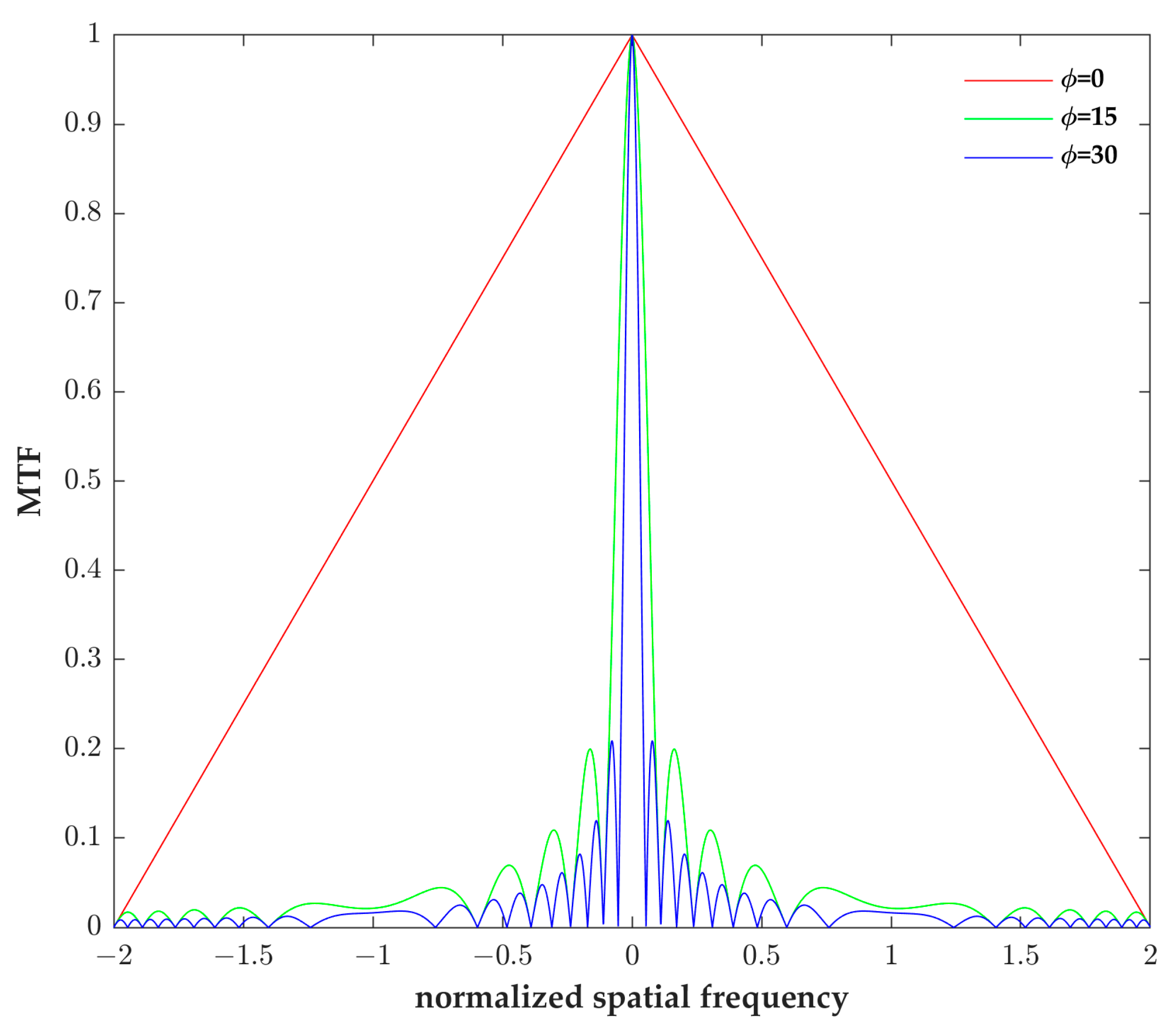
Figure 2 shows the MTF curve of an ideal optical system at a different defocus aberration $\varphi$. As shown in Figure 2, the system establishes a clear image at the defocus aberration $\varphi =0$. With the increase in defocus aberration, the MTF curve of the system changes more obviously, the MTF value drops more rapidly, and a result of zero occurs, leading to losses of image information.

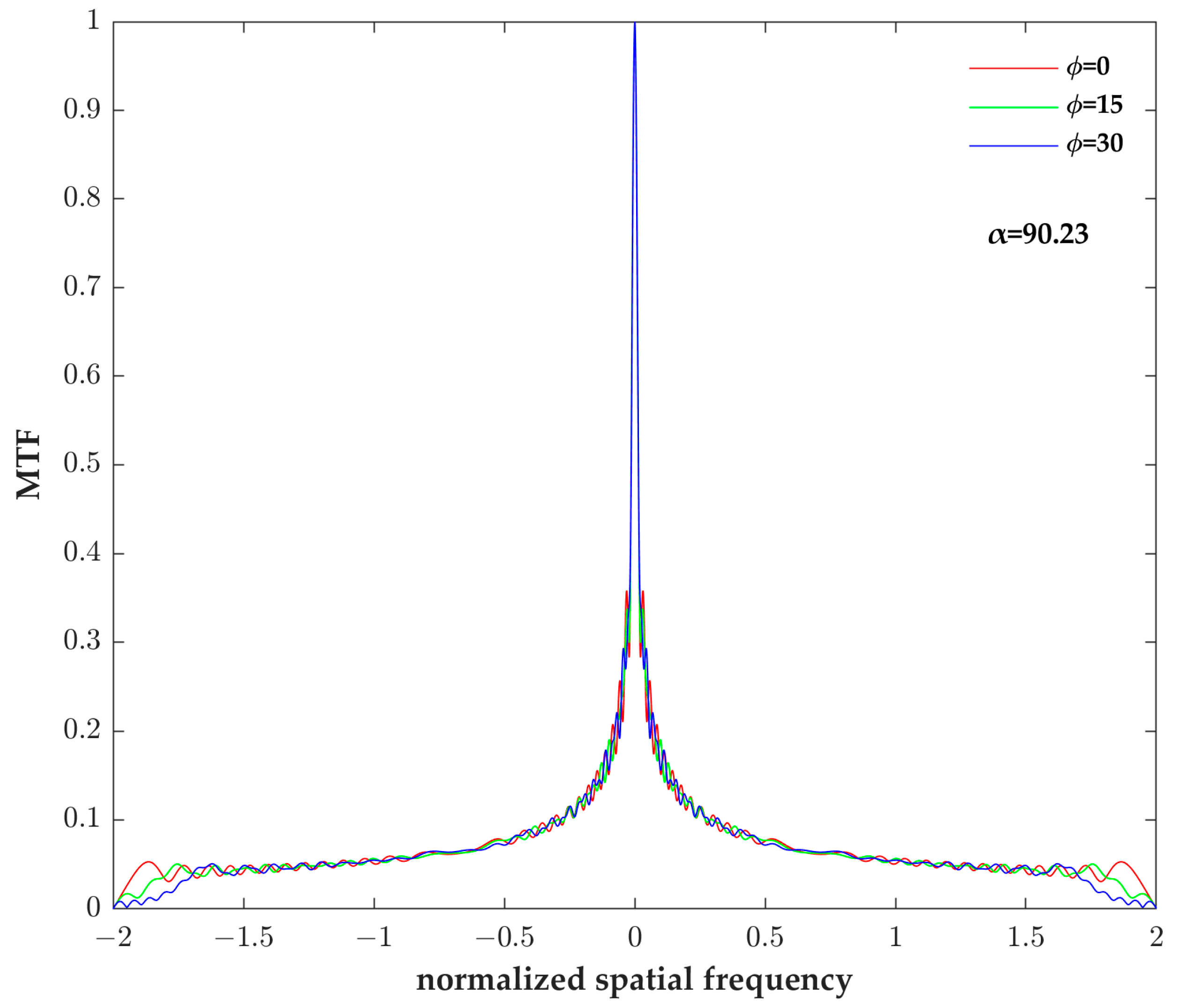
The optimized result 90.23 in the fourth row of Table 2 was taken as the cubic phase mask parameter, and this cubic phase mask was added to the ideal optical system in Figure 2. As shown in Figure 3, after optimizing the phase mask parameter obtained by the improved PSO, the MTF curves of the wavefront coding system under the different defocus aberrations are almost the same, and there are no zero points. This proves that the current system can achieve defocus insensitivity under different defocus aberrations, that is, realize the DoF extension of the current system. This also proves that the improved PSO can optimize a reasonable cubic phase mask parameter.

3.2. Comparison of Improved PSO and Traditional PSO

Table 3. Comparison of improved PSO and traditional PSO.

Parameter	Avg	Var	Average Time/s	References
$v_{\max }=0.7;v_{\min }=-0.7$	70.71	0.27	5.96	[8]
$v_{\max }=0.8;v_{\min }=-0.8$	80.70	0.23	5.94	[8]
$v_{\max }=0.9;v_{\max }=-0.9$	90.58	0.53	5.98	[8]
$v_{\max }=1.0;v_{\max }=-1.0$	100.77	0.19	6.08	[8]
$\mathrm{T}=0.15$	90.23	7.40 × 10−3	5.90	this work

shows a comparison of improved PSO and traditional PSO. In Table 3, $v_{\max }$ represents the maximum velocity, and $v_{\min }$ represents the minimum velocity. For the convenience of comparison, some parameters of improved PSO and traditional PSO were set as the same: the number of particles $D=30$ and the number of iterations $I=100$. In Table 3, the data from rows 2 to 5 are the traditional PSO with different velocity ranges and without threshold $\mathrm{T}$. The data in row 6 are the improved PSO when cancelling the setting of velocity ranges and using threshold $\mathrm{T}=0.15$.

It can be seen from Table 3 that when using traditional PSO, the range of velocity has a great influence on the optimal solution. A large or small range of velocity will cause PSO to fall into the local optimal solution. Therefore, it is necessary to repeatedly try different velocity value ranges to obtain a more appropriate cubic phase mask parameter. However, the improved PSO does not need to set the velocity ranges, and furthermore, a threshold is introduced to ensure the quality of image restoration and improve the stability of optimization.

The improved PSO avoids the disadvantages of the traditional PSO, which requires multiple tests to obtain the appropriate range of velocity. Therefore, the improved PSO avoids the problem of falling into the local optimal solution in the optimization process, and its robustness is significantly improved.

3.3. Comparison between Improved PSO and SA

The simulated annealing algorithm (SA) [5], one of the most widely used optimization algorithms, is applied for comparison to demonstrate the efficiency and robustness of PSO.

In SA, $T_{\max }$ represents the maximum temperature, $T_{\min }$ represents the minimum temperature, $r$ represents the cooling rate, and $K$ represents the number of temperature iterations.

During the process of finding the optimal solution, SA accepts not only the current optimal solution but also the bad solution with a certain probability. This strategy is the key to causing SA to jump out of the local optimal solution. However, due to the many parameters of SA, the improper setting of these parameters will cause SA to fall into local optimal solutions or take more time to obtain a stable optimal solution.

To facilitate comparison, Equation (3) was used for both the improved PSO and SA as the evaluation function when defocusing the insensitivity of the current wavefront coding system, and threshold $\mathrm{T}$ was introduced into SA.

Table 4. Influence of the cooling rate and the number of temperature iterations on SA.

Parameter	Avg	Var	Average Time/s
$\mathrm{r}=0.90;K=100$	89.77	0.17	57.97
$\mathrm{r}=0.90;K=10$	86.31	9.41	5.53
$\mathrm{r}=0.60;K=100$	88.08	4.93	11.44
$\mathrm{r}=0.30;K=100$	86.57	9.13	5.02
$\mathrm{r}=0.30;K=10$	66.75	2.44 × 102	0.45

The data in Table 4 are based on $T_{\max }={10}^3$ and $T_{\min }={10}^{-12}$. This method is based on reference [5].

and

Table 5. Influence of the maximum temperature and the minimum temperature on SA.

Parameter	Avg	Var	Average Time/s
$T_{\max }={10}^2;T_{\min }={10}^{-12}$	89.89	0.16	58.67
$T_{\max }=10;T_{\min }={10}^{-12}$	89.81	0.26	58.86
$T_{\max }={10}^3;T_{\min }={10}^{-1}$	18.16	2.72 × 102	8.29
$T_{\max }={10}^3;T_{\min }={10}^{-6}$	88.22	3.67	31.74
$T_{\max }=10;T_{\min }={10}^{-1}$	16.96	2.53	8.27

The data in Table 5 are based on $r=0.9$ and $K=100$. This method is based on reference [5].

show the influence of all parameters on SA. For details of the phase mask design based on SA, please refer to Appendix A.

In Table 4, with the decrease in cooling rate $r$ and the number of temperature iterations $K$, the solution easily falls into the local optimal solution when the maximum temperature $T_{\max }$ and the minimum temperature $T_{\min }$ are constants. If the cooling rate $r$ and the number of temperature iterations $K$ are increased, the optimization time will be increased.

In Table 5, $T_{\min }$ has a greater influence on the optimization result than $T_{\max }$. SA easily falls into the local optimal solution when $T_{\min }$ increases. Additionally, the program runtime will increase when $T_{\min }$ decreases.

In contrast, the improved PSO is robust and easy to use. For the optimization of the cubic phase mask, the runtime of the improved PSO is only related to the population of particles $D$ and the number of iterations $I$.

Table 6. The influence of the population of particles and the number of iterations on the improved PSO.

Parameter	Avg	Var	Average Time/s
$D=20;I=100$	90.19	2.14 × 10−2	3.97
$D=10;I=100$	90.07	6.61 × 10−2	1.97
$D=30;I=10$	89.42	1.00	0.64
$D=30;I=100$	90.23	7.40 × 10−3	5.900
$D=10;I=10$	87.64	7.73	0.22

shows the influence of the population of particles and the number of iterations on the improved PSO. With the appropriate population of particles and number of iterations, the algorithm can obtain a stable optimal solution within a short time. As shown in the data in row 5 of Table 6, when $D=30$ and $I=100$, the average value of the cubic phase mask optimized by the improved PSO is 90.23, the variance is only 7.40 × 10⁻³, and the average time is only 5.90 s.

4. Experimental Results

To verify the correctness of the improved particle swarm optimization results, the optimized cubic phase mask is used in an actual wavefront coding system for DoF extension experiments. The optimized result 90.23 is taken as the cubic phase mask parameter in the experiment. Note that the cubic phase mask parameter is optimized in normalized coordinates. Taking 90.23 as an example, the maximum phase modulation at the edge of the pupil, i.e., $x=\pm 1$, is 90.23 according to Equation (1). A spatial light modulator (SLM) is used to generate a cubic phase mask with a size of $15.36 \mathrm{m}\mathrm{m}\times 8.64 \mathrm{m}\mathrm{m}$. Assuming that the maximum phase modulation at the long edge remains unchanged, the cubic phase mask parameter of the actual system can be converted to 0.20, which is the actual phase mask parameter used in the experiment. The two-dimensional cubic phase mask $f(x,y)$ can be described as

$$f\left(x,y\right)=\alpha \left(x^3+y^3\right)$$

(7)

where $x$ and $y$ are the coordinates of the phase mask. Let the center of the cubic phase mask be the origin of the coordinates, then the range of values of x and y are $-7.68 \mathrm{m}\mathrm{m}\le x\le 7.68 \mathrm{m}\mathrm{m}$ and $-4.32 \mathrm{m}\mathrm{m}\le y\le 4.32 \mathrm{m}\mathrm{m}$, respectively. The pupil function, which ignores all optical aberrations but defocus, can be described as

$$p\left(x,y\right)=\exp \left[\mathrm{j}\left(f\left(x,y\right)+\varphi \left(x^2+y^2\right)\right)\right]$$

(8)

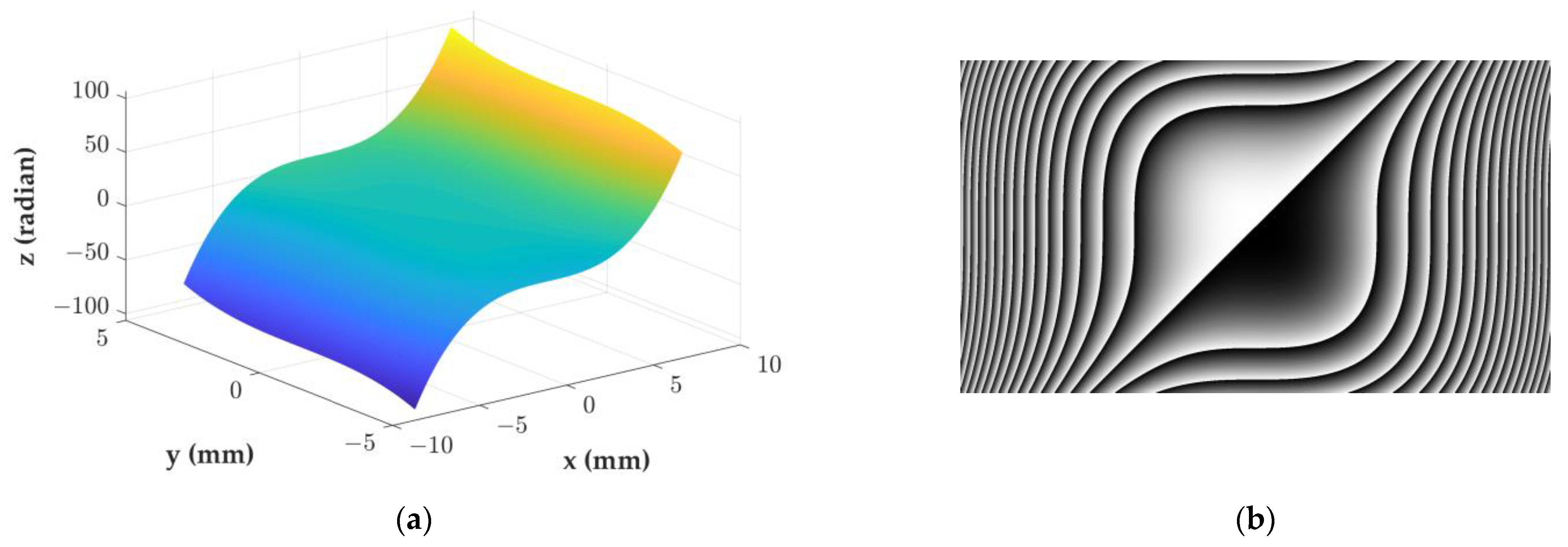
where $\varphi$ is the defocus aberration and $\mathrm{j}$ is the imaginary unit. Figure 4a shows a three-dimensional plot of the actual cubic phase mask, with the x and y axes corresponding to the spatial coordinates, respectively, and the z axis indicating the phase. Its corresponding contour map of the surface of the cubic phase mask is shown in Figure 4b.

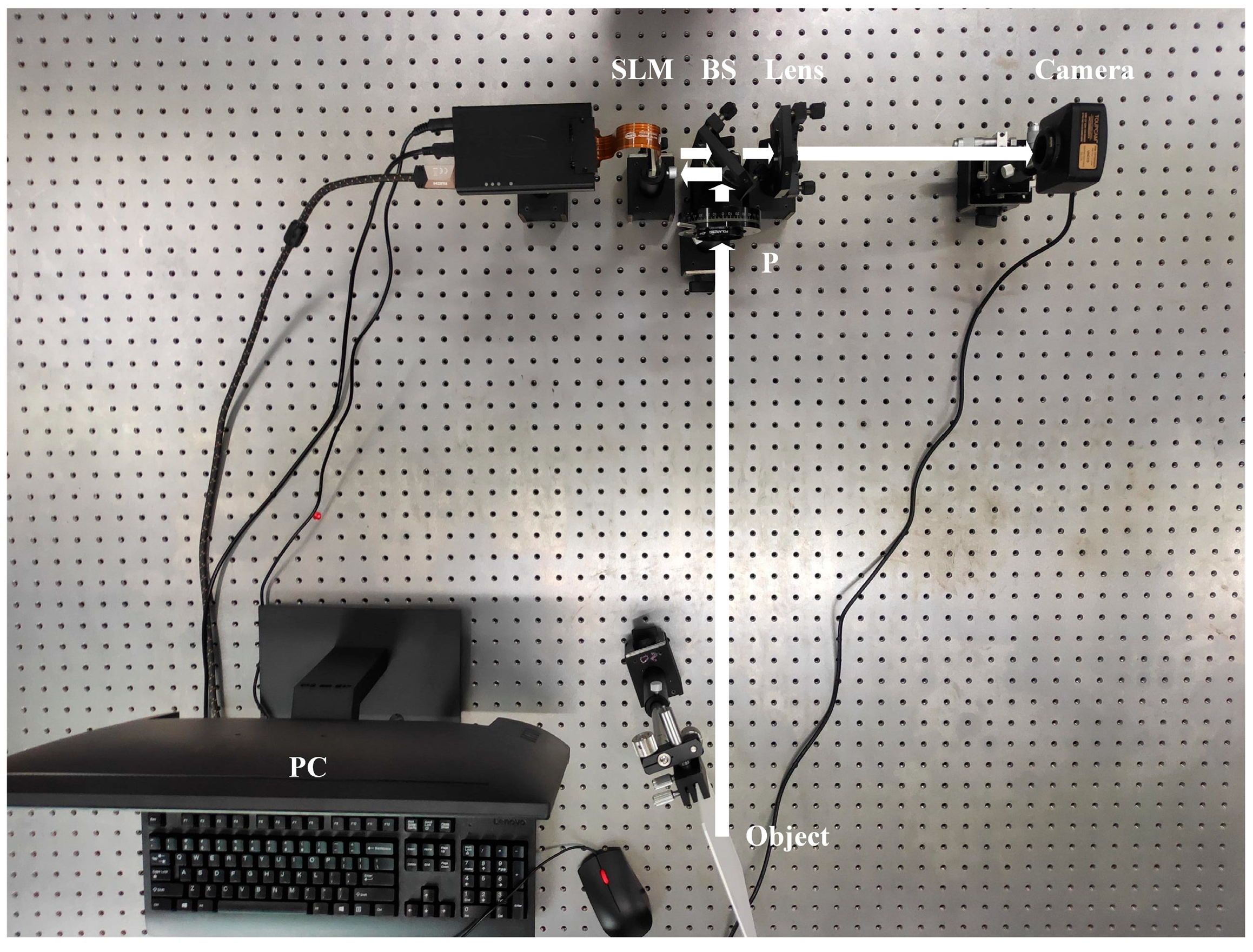
Figure 5 shows a DoF extended wavefront encoding system, where the light diffusely reflected from the object passes through the polarizer (P) and arrives at the spatial light modulator (SLM) after being reflected by the beam splitter (BS). The light, which is modulated by the SLM, passes through the BS and is imaged on the camera by the lens. P works in conjunction with SLM to achieve cubic phase modulation. A tilted ruler is used as a large DoF object, as shown as the object of Figure 5.

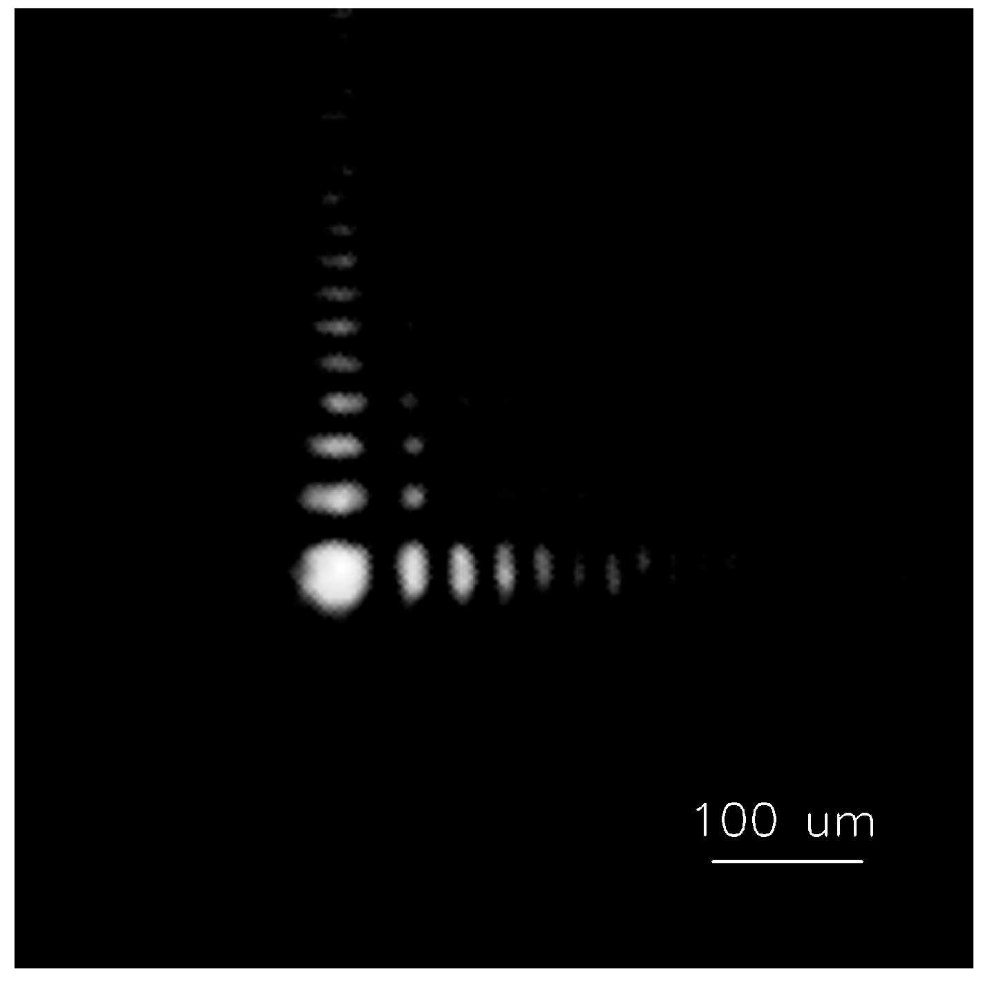
The measured PSFs are almost identical at defocus amounts of 0, 15, and 30, and the focused PSF is given in Figure 6.

Since the PSFs are consistent for different defocus amounts, the wavefront encoding system has the same degree of blurring for different defocus objects. This makes it possible to use the same PSF for image recovery in later stages.

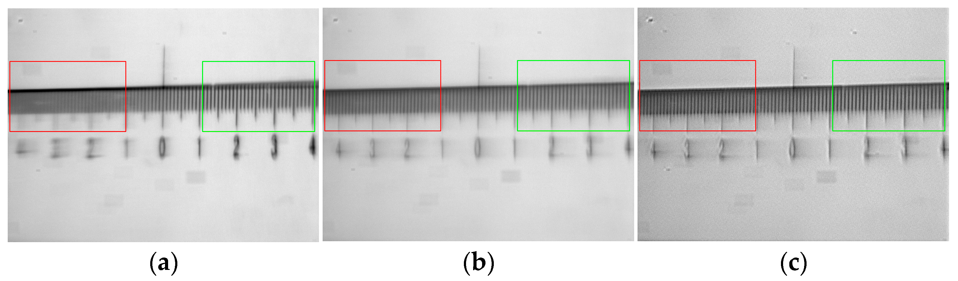
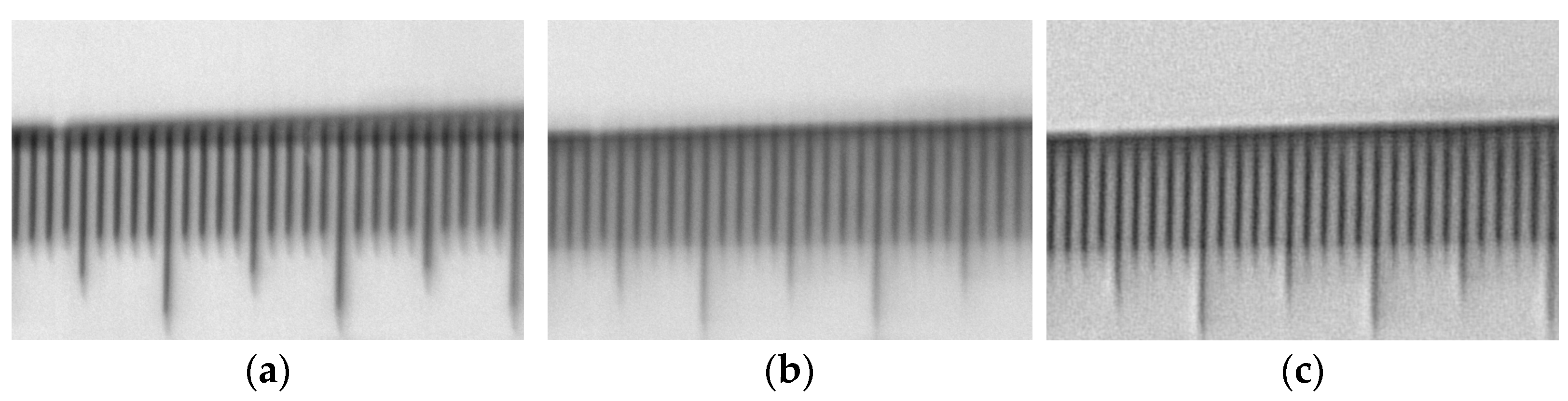
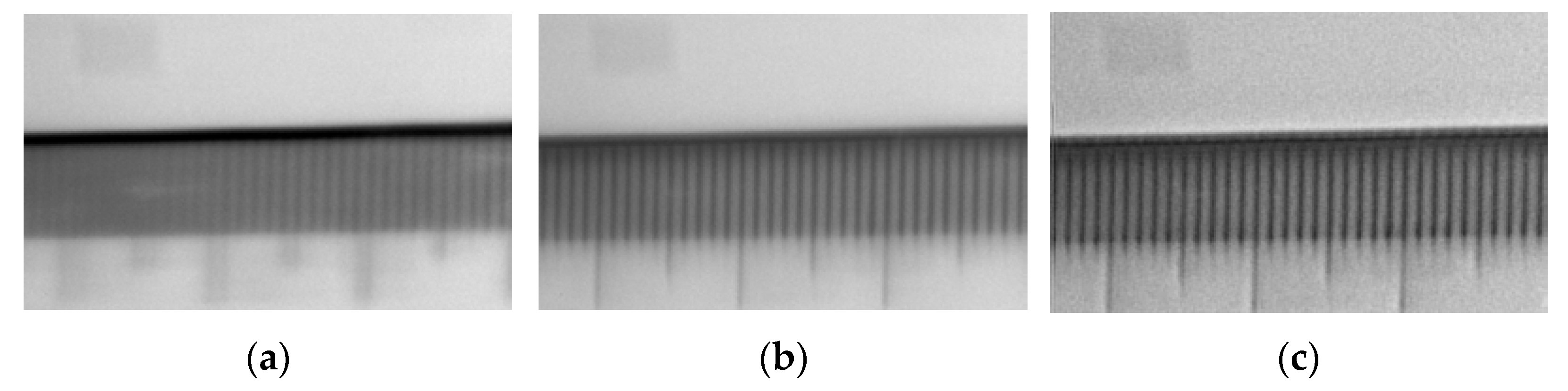
To demonstrate the DoF extension effect of the wavefront encoding system, a conventional imaging system is built to image objects with a large DoF for comparison. The conventional imaging results for a tilted scale are shown in Figure 7a, where the object is clearly imaged at the focus (0~1 mm), but the object is gradually blurred at the front defocus (shown in the green box) and the back defocus (shown in the red box). The magnified images of the front defocus and back defocus parts are shown in Figure 8 and Figure 9, respectively, which show that the objects are gradually blurred or even indistinguishable as the defocus amount increases.

The imaging results of the wavefront coding system modulated by the cubic phase mask are shown in Figure 7b. Although there is some blurring at the focus, the blurring degree at the front and back defocus is improved compared with the conventional imaging system, and the blurring degree is thought to be consistent at different positions. The PSF shown in Figure 6 is used as the convolution kernel, and the Wiener filter [16] is used as the decoding method. The decoded image is shown in Figure 7c. Like Figure 7a, we zoomed in to show the front defocus (shown in the green box) and back defocus (shown in the red box) of the intermediate image shown in Figure 7b and the decoded image shown in Figure 7c. Figure 8a–c show the image of the conventional optical system, the intermediate image, and the decoded image of the wavefront coding system at the front defocus, respectively. Figure 9a–c show the image of the conventional optical system, the intermediate image, and the decoded image of the wavefront coding system at the back defocus, respectively. The wavefront coding system distinguishes details that cannot be resolved by the conventional imaging optical imaging system at the front and back defocus.

The experimental results indicate that the phase mask optimized by the improved particle swarm algorithm achieved the DoF extension in the wavefront coding system.

5. Conclusions

The phase mask design proposed in this paper is based on the improved PSO. The improved PSO uses the coincidence of MTF curves under different defocus aberrations to evaluate the defocus insensitivity of MTF. At the same time, the value range of velocity is cancelled, the threshold is introduced, and the cubic phase mask parameter is successfully optimized. The improved PSO eliminates the influence of the velocity value range and has better robustness. After a simple adjustment of the population of particles and the number of iterations, the optimal solution of the cubic phase mask parameter can be quickly and effectively obtained. The experimental results verify that the cubic phase mask optimized by the improved particle swarm algorithm can achieve DoF extension in the wavefront coding system. In this study, a one-dimensional simplified analysis of cubic phase masks was carried out, and the method can be extended to two-dimensional phase masks, as well as to the optimization problems of other types of phase masks, such as logarithmic phase masks, sinusoidal phase masks, tangent phase masks, and exponential phase masks.

References

- Dowski, E.R.; Cathey, W.T. Extended depth of field through wave-front coding. Appl Opt. 1995, 34, 1859–1866. [Google Scholar] [CrossRef] [PubMed] [Green Version]
- Yang, L.; Chen, M.; Wang, J.; Zhu, M.; Yang, T.; Zhu, S.; Xie, H. Extended Depth-of-Field of a Miniature Optical Endoscope Using Wavefront Coding. Appl. Sci. 2020, 10, 3838. [Google Scholar] [CrossRef]
- Lee, C.F.; Lee, C. Microscope with Extension of the Depth of Field by Employing a Cubic Phase Plate on the Surface of Lens. Results Opt. 2021, 4, 100107. [Google Scholar] [CrossRef]
- Yu, J.; Chen, S.; Dang, F.; Li, X.; Shi, X.; Wang, H.; Fan, Z. The suppression of aero-optical aberration of conformal dome by wavefront coding. Opt. Commun. 2021, 490, 126876. [Google Scholar] [CrossRef]
- Zhu, L.; Li, F.; Huang, Z.; Zhao, T. An apodized cubic phase mask used in a wavefront coding system to extend the depth of field. Chin. Phys. B 2022, 31, 054217. [Google Scholar] [CrossRef]
- Li, Y.; Wang, J.; Zhang, X.; Hu, K.; Ye, L.; Gao, M.; Cao, M.; Cao, Y.; Xu, M. Extended depth-of-field infrared imaging with deeply learned wavefront coding. Opt. Express 2022, 30, 40018–40031. [Google Scholar] [CrossRef] [PubMed]
- Kennedy, J.; Eberhart, R. Particle Swarm Optimization. In Proceedings of the ICNN‘95—International Conference on Neural Networks, Perth, Australia, 27 November–1 December 1995. [Google Scholar]
- Eberhart, R.C.; Kennedy, J. A New Optimizer Using Particle Swarm Theory. In Proceedings of the Micro Machine and Human Science 1995, MHS ‘95, Sixth International Symposium, Nagoya, Japan, 4–6 October 1995. [Google Scholar]
- Castro, A.; Ojeda-Castaneda, J. Increased depth of field with phase-only filters: Ambiguity function (Invited Paper). In Proceedings of the SPIE OPTO—Ireland, Dublin, Ireland, 5–6 April 2005. [Google Scholar]
- Yang, Q.; Liu, L.; Sun, J. Optimized phase pupil masks for extended depth of field. Opt. Commun. 2007, 272, 56–66. [Google Scholar] [CrossRef]
- Wang, J.; Bu, J.; Wang, M.; Yang, Y.; Yuan, X.-C. Improved sinusoidal phase plate to extend depth of field in incoherent hybrid imaging systems. Opt. Lett. 2012, 37, 4534–4536. [Google Scholar] [CrossRef] [PubMed]
- Ma, Z.; Li, Y. Parameter extraction and inverse design of semiconductor laser based on deep learning and particle swarm optimization method. Opt. Express 2020, 28, 21971–21981. [Google Scholar] [CrossRef] [PubMed]
- Lee, C.Y.; Le, T.A. Intelligence Bearing Fault Diagnosis Model Using Multiple Feature Extraction and Binary Particle Swarm Optimization with Extended Memory. IEEE Access 2020, 8, 198343–198356. [Google Scholar] [CrossRef]
- Li, J.; Dong, X.; Ruan, S.; Shi, L. A parallel integrated learning technique of improved particle swarm optimization and BP neural network and its application. Sci. Rep. 2022, 12, 19325. [Google Scholar] [CrossRef]
- Eberhart, R.C.; Shi, Y. Particle swarm optimization: Developments, applications and resources. In Proceedings of the 2001 Congress on Evolutionary Computation, Seoul, Republic of Korea, 27–30 May 2001. [Google Scholar]
- Bradburn, S.; Cathey, W.T.; Dowski, E.R. Realizations of focus invariance in optical–digital systems with wave-front coding. Appl. Opt. 1997, 36, 9157–9166. [Google Scholar] [CrossRef]
Figure 1.
Flow diagram of phase mask design based on improved PSO.
Figure 2.
The MTF curve of an ideal optical system before adding the cubic phase mask.
Figure 3.
The MTF curves of wavefront coding systems with the cubic phase mask.
Figure 4.
The profiles of the cubic phase mask used in the experiment: (a) three-dimensional cubic phase mask; and (b) the contour map of the surface of the cubic phase mask.
Figure 5.
Wavefront coding system, including spatial light modulator (SLM) with size
and resolution ; beam splitter (BS); polarizer (P); observation object (Object); lens (Lens) with focal length 200 mm; and camera (Camera).
Figure 6.
PSF of wavefront coding system.
Figure 7.
Imaging comparison chart of conventional optical system and wavefront coding system. (a) Conventional optical system. (b) Intermediate image captured by wavefront coding system. (c) Decoded image from intermediate image.
Figure 8.
Magnified image at the front defocus (green box in Figure 7). (a) Image of the conventional imaging system. (b) Intermediate image of the wavefront coded imaging system. (c) Decoded image of the wavefront coded system.
Figure 9.
Magnified image at the back defocus (red box in Figure 7). (a) Image of the conventional imaging system. (b) Intermediate image of the wavefront coded imaging system. (c) Decoded image of the wavefront coded system.