
Modeling of the German Wind Power Production with High Spatiotemporal Resolution


1
Department of Bioenergy, Helmholtz Centre for Environmental Research GmbH—UFZ, Permoserstraße 15, 04318 Leipzig, Germany
2
Bioenergy Systems Department, DBFZ Deutsches Biomasseforschungszentrum gGmbH, Torgauer Str. 116, 04347 Leipzig, Germany
*
Author to whom correspondence should be addressed.
ISPRS Int. J. Geo-Inf. 2021, 10(2), 104; https://0-doi-org.brum.beds.ac.uk/10.3390/ijgi10020104
Submission received: 21 December 2020
/
Revised: 10 February 2021
/
Accepted: 14 February 2021
/
Published: 23 February 2021
(This article belongs to the Collection Spatial and Temporal Modelling of Renewable Energy Systems)
Abstract
:Wind power has risen continuously over the last 20 years and covered almost 25% of the total German power provision in 2019. To investigate the effects and challenges of increasing wind power on energy systems, spatiotemporally disaggregated data on the electricity production from wind turbines are often required. The lack of freely accessible feed-in time series from onshore turbines, e.g., due to data protection regulations, makes it necessary to determine the power generation for a certain region and period with the help of numerical simulations using publicly available plant and weather data. For this, a new approach is used for the wind power model which utilizes a sixth-order polynomial for the specific power curve of a turbine. After model validation with measured data from a single wind turbine, the simulations are carried out for an ensemble of 25,835 onshore turbines to determine the German wind power production for 2016. The resulting hourly resolved data are aggregated into a time series with daily resolution and compared with measured feed-in data of entire Germany which show a high degree of agreement. Such electricity generation data from onshore turbines can be applied to optimize and monitor renewable power systems on various spatiotemporal scales.
1. Introduction
Despite its volatility, renewable energy from wind turbines has become an essential pillar for the electricity supply in many countries around the world. During the past decade, wind power continued its strong forward momentum with significant advances in grid integration and cost reduction. For example, 60.4 GW of new wind turbine capacity was installed worldwide in 2019, the second highest value in history and close to the 2015 peak of 63.8 GW, leading to a total volume of 651 GW [1]. The German onshore capacity has increased from 6.1 GW in the year 2000, when the German Renewable Energy Act (EEG) was introduced, to 53.3 GW at the end of 2019 [2]. These numbers are expected to rise in the future due to the decreasing levelized costs of electricity [3] and the needed further de-carbonization of the power sector to achieve the currently set climate targets in Germany, e.g., reducing greenhouse gas emissions by at least 55% below 1990 levels by 2030, according to the Federal Climate Change Act (KSG 2019).
The rapid advancement of variable renewable energies like wind power not only has an essential impact on the future development of power grids but on many other fields of the energy sector as well, triggering the need for further research. Thus far, current energy studies for Germany often contain the electricity production from wind turbines with a high spatial resolution, but lack a high temporal resolution, such as the energy transition analysis of the power sector [4]. On the other hand, there are also wind power simulations available, such as the potential analysis for hybrid renewable energy systems in Central Europe [5,6], which already provide a high spatiotemporal resolution using highly resolved weather data but cannot represent this information for existing wind turbines due to the lack of detailed plant datasets. In order to gain a better understanding of the effects and challenges caused by a growing share of variable renewables on energy systems, high spatiotemporal distributions of the power generation, e.g., down to municipal and hourly resolutions, will increasingly become a crucial factor for future research. Especially, energy studies on decentralized power systems with many renewable power plants can benefit from this information, e.g., to prevent possible power shortages induced by regional dark doldrums or local component failures [7]. However, the lack of disaggregated electricity production data for a certain region and period, e.g., due to strict data protection regulations, makes it difficult for decision makers and researchers to investigate the multiple effects of increasing wind power on a regional or local scale.
This publication presents a new approach for creating power generation data of wind turbines with a high spatiotemporal resolution, which can help to close the previously mentioned gap. Up to now, energy transition maps have been developed to support decision makers and researchers with such data down to the municipal level [4], but only on the basis of an annual power production from onshore turbines. In order to be able to generate this information also for a shorter period of time, spatiotemporally resolved data are necessary, which are made possible with the presented model approach using publicly available plant and weather data.
The remainder of this paper is organized as follows: Section 2 introduces the used plant and weather data, as well as the information needed for calibration and validation of the simulations. The wind power model, which is a further development of our physical model presented in [8], and its implementation are described in Section 3. In Section 4, this simulation model is applied to a measured single turbine and, subsequently, to an ensemble of 25,835 onshore turbines located in Germany. Afterwards, the resulting time series from the numerical simulations are aggregated and compared with measured feed-in data for the validation. Section 5 discusses the performed simulations and introduces the first utilization examples using the obtained results. Last but not least, this study ends with brief conclusions in Section 6.
2. Data
The following subsections describe all the data required for the simulation model including their origin and properties.
2.1. Plant Dataset
The initial wind turbine dataset originates from the EE-monitor project [9], which is freely accessible via the data research portal (www.ufz.de/drp (accessed on 5 March 2020)) of the UFZ. This dataset, with detailed onshore turbine information including the geographical location, installed capacity, hub height, rotor diameter, and the year of commissioning until end of the year 2015, was compiled from official sources of the federal states of Germany [10]. As known from plant-related studies [10,11,12], wind turbine datasets for larger regions or an entire country are rarely complete due to the high number of plants with many specific parameters. That is why different procedures were developed to complete such turbine datasets as much as possible. For the turbine data of the EE-monitor project, the method of random forests was applied to generate the missing information [13], e.g., to reconstruct an unknown hub height of a certain turbine by the other available parameters. In order to extend this plant dataset to all federal states and update it to the year 2016, the wind turbines of the German city states and the onshore turbines erected in 2016 were inserted by using additionally requested data from official sources. Finally, all wind turbines of this dataset were compared with the Core Energy Market Data Register [14] by a spatial join. If the turbine locations were nearly identical in this operation, i.e., showing a spatial deviation smaller than 75 m in both data sources, the corresponding turbine data of the plant dataset were supplemented with information from the Core Energy Market Data Register. This join has often inserted the exact hub height instead of the estimated value generated by the random forests method, the date of (de-)commissioning, and the turbine type into the dataset. Thus, in many cases, the actual date of (de-)commissioning can be used instead of the less precise commissioning year, which enables the wind power model to consider the intra-annual plant changes. After these improvements and filtering the data by wind turbines operated in the investigated year 2016, the final plant dataset consists of 25,835 onshore turbines corresponding to a total capacity of 43.61 GW. This value is in good agreement with the officially installed capacity of 45.28 GW of all onshore turbines in Germany for 2016 [2]. The small deviation of less than 3.7% from the official sum indicates that most wind turbines are included in the final dataset.
For each turbine, the plant dataset contains the geographical position using the latitude and longitude coordinates, the associated local administrative unit (LAU)-Id 1, rated power, hub height, turbine type, and the date of (de-)commissioning, as shown in Table 1. It should be stated, that the rotor diameter of a wind turbine is not needed for the model approach introduced in this study, and therefore all uncertainties regarding this parameter do not influence the simulation results.
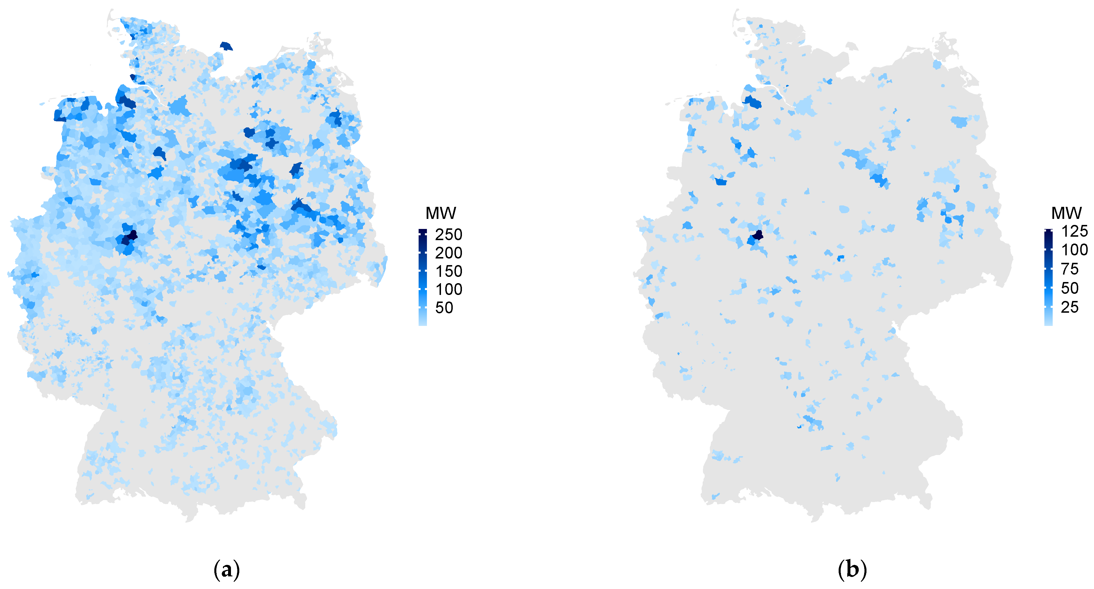
Figure 1 shows the installed capacity of the wind turbines at the spatial resolution of LAU2 in Germany for 2016 and, as additional information, the intra-annual capacity increase during this time.
2.2. Calibration Data
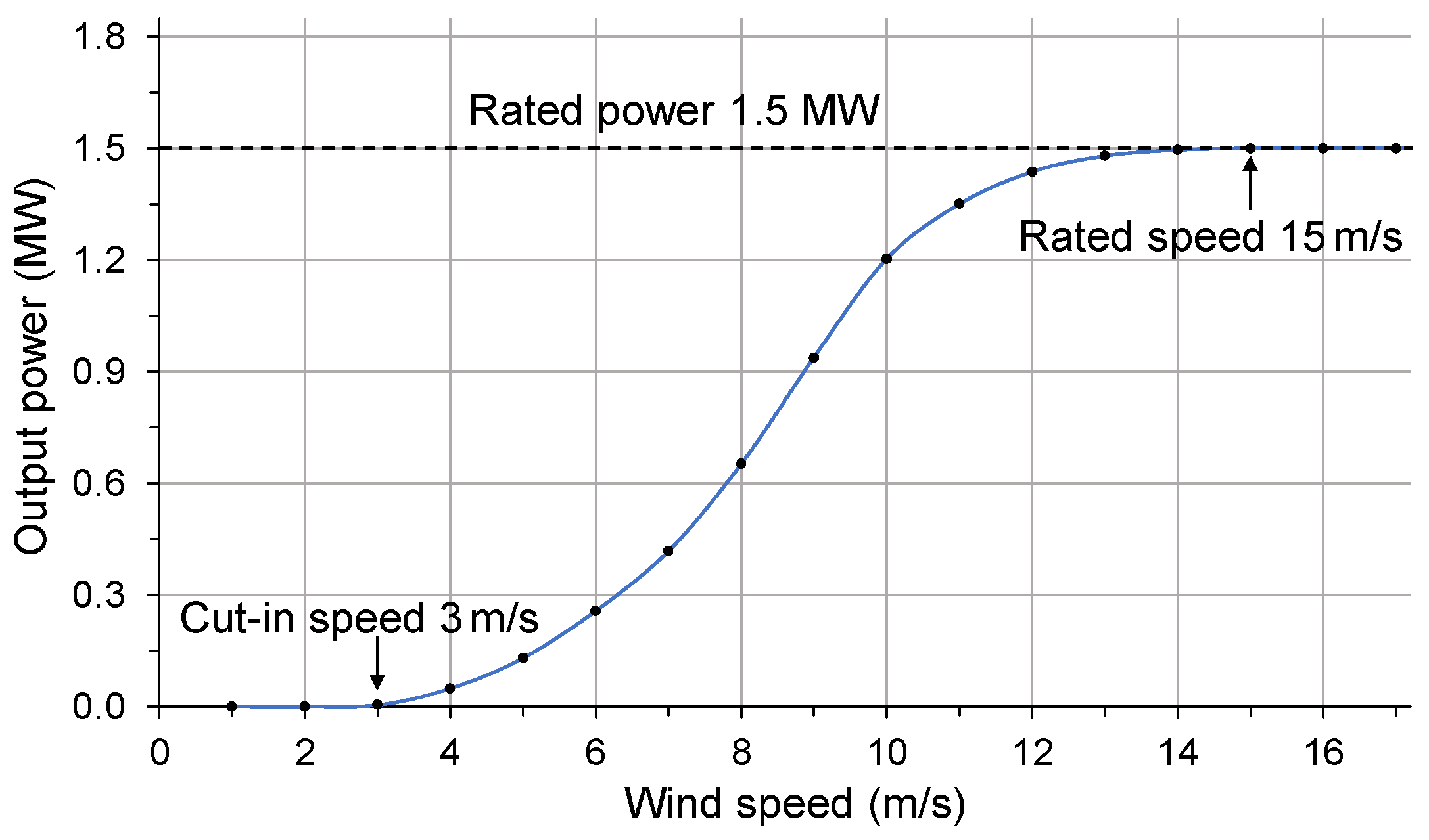
For a reasonable calibration of the wind power model, further information is required, which is not included in the plant dataset shown in Table 1. For the presented simulation model, the data of the specific power curve of a wind turbine, including its characteristic cut-in, rated, and cut-out speed, are necessary. Such power curves, which show the relationship between the wind speed at hub height and the output power at a standardized air density of 1.225 kg/m3, are available in the technical datasheets of the turbine manufacturer or can be found on internet platforms, e.g., at The Wind Power (www.thewindpower.net) [15].
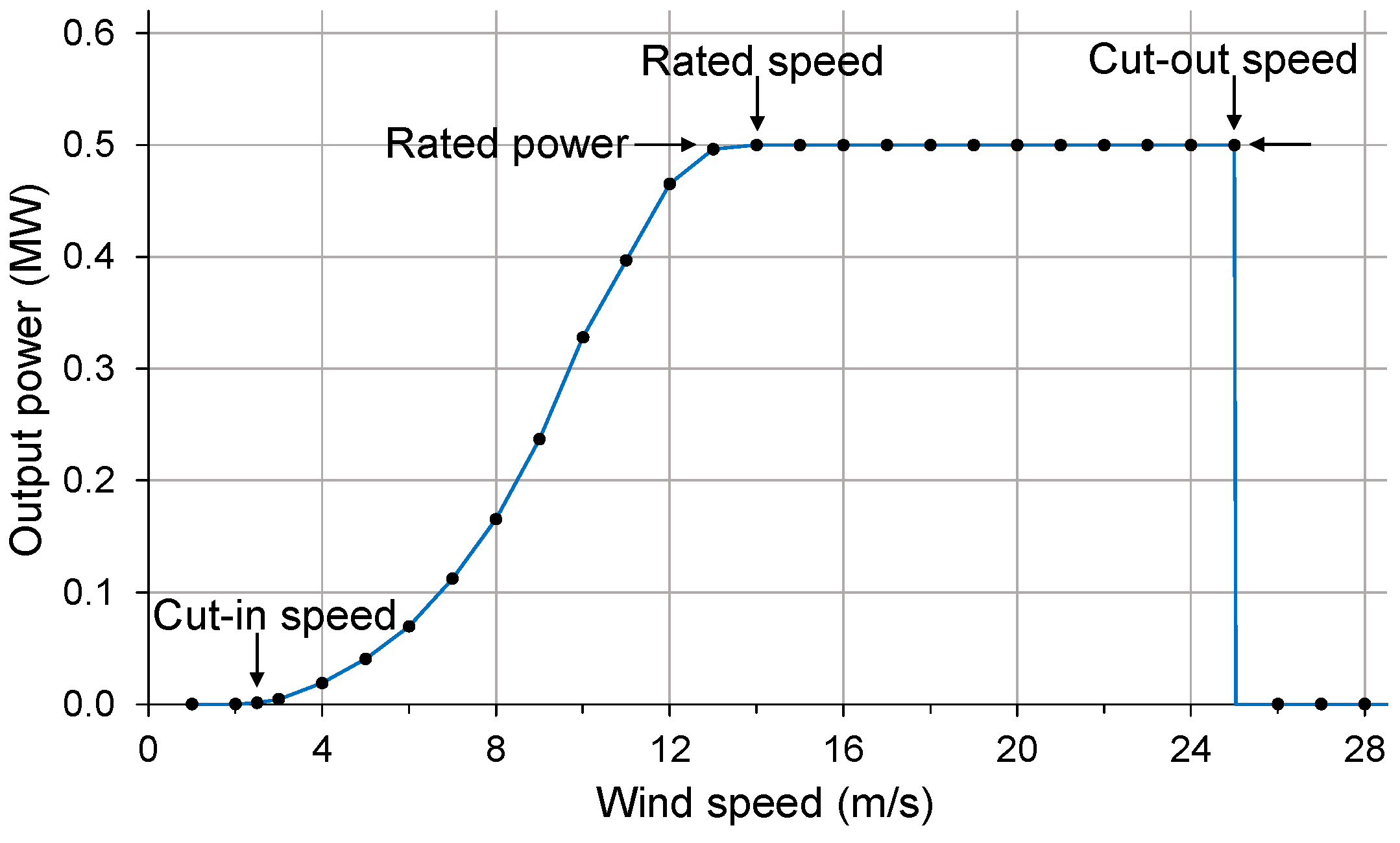
The graph in Figure 2 shows the typical power curve of a pitch-controlled wind turbine with its characteristic parameters.
At wind speeds below the cut-in speed (vcut-in) there is insufficient torque exerted by the wind stream on the turbine blades to make them rotate. However, when the wind speed increases, the turbine begins to rotate and generates electricity. The wind speed when the turbine starts to deliver energy into the power grid is called cut-in speed. For most wind turbines it is between 2 and 4 m/s. When the wind speed rises above this cut-in speed, the level of the generated electricity increases rapidly. Typically, somewhere in the range of 12 and 14 m/s, the electrical output reaches the nominal value that the wind turbine is designed for. This value is called rated power (PR) and the concerning wind speed is the rated speed (vrated). At higher wind speeds, the turbine is designed to limit the output to this level. How this behavior is done depends on the technical design, but for most onshore turbines, it is achieved by adjusting the blade angles depending on the wind speed to keep the electrical output constant. This kind of power regulation is called pitch control. When the wind speed increases well above the rated speed, the forces on the turbine structure continue to rise and, at some point, there is a risk of damage. As a result, a switch-off and braking system is employed to bring the rotor to a standstill. The wind speed required for a switch-off is called cut-out speed (vcut-out) which is about of 25 m/s for many onshore turbines.
For losses of wind turbines, which cannot be captured by calculations based on the power curve, an additional reduction of the produced electricity has to be considered in the numerical simulations. Such losses are caused, e.g., by the following effects:
- Power losses due to mutual shading of adjacent turbines (wake effect).
- Switch-offs due to wind turbine revisions or bird and bat protection.
- Feed-in interruptions due to energy surpluses in the power grids.
Due to the lack of this information on each wind turbine, this kind of turbine losses is included in the wind power model as an averaged overall value for the entire plant ensemble.
2.3. Weather Database
High-resolution weather data are a key requirement for modeling the power production from wind turbines and, herein, the data quality plays an important role for the accuracy of the performed simulations. For the region of Central Europe or Germany, various weather products with different spatiotemporal resolutions are freely accessible via the web interfaces of many meteorological services. So-called reanalysis products have emerged as a popular source of weather data for various electricity generation studies, especially for wind power modeling [11,17,18,19,20]. Such reanalysis weather data are calculated using numerical forecast models, re-running these weather models for a certain period in the past, and making corrections with existing meteorological measurements. In general, the spatial resolutions of global reanalysis data, e.g., the MERRA and MERRA-2 products with a resolution of about 50 km [21,22], are not sufficient for the level of detail needed for this paper. In contrast to global weather products, regional reanalysis data have typically higher spatial resolutions, e.g., the COSMO-REA6 weather data covering Europe with a spatial resolution of about 6 km [23], and, therefore, would already allow detailed simulation results with our wind power model.
This publication goes a step further and uses satellite-based weather data from the Satellite Application Facility on Climate Monitoring (CMSAF) collaboration [24] via the open-access web interface of the Photovoltaic Geographical Information System (PVGIS) [25]. The CMSAF database in PVGIS has a temporal resolution of an hour and a spatial resolution of about 2.5 km for the region of Germany according to [25]. The delivered hourly resolved time series for a required location and period contains the following information relevant for the simulation model: date and time in coordinated universal time (UTC), ground elevation, ambient temperature at 2 m, and the total wind speed at 10 m above ground level. Although the wind speed is only available at 10 m in PVGIS, which may reduce the accuracy of the wind speed extrapolation to the required hub height of the onshore turbines, the weather data are retrieved individually for each plant location. This circumstance avoids additional spatial interpolations of weather data to the specified turbine sites and, therefore, the uncertainties caused by such routines. Moreover, PVGIS also provides the ground elevation at the plant location needed for the calculation of air pressure as a function of the total height above sea level. Thus, the CMSAF weather product via PVGIS 5.1 was used for the simulation of the German wind power production. In addition, the wind power model and the already published photovoltaic model [26] can be used together with the same weather product in PVGIS, which improves the mutual combinability of the simulation results, e.g., because they have the same time base.
2.4. Validation Data
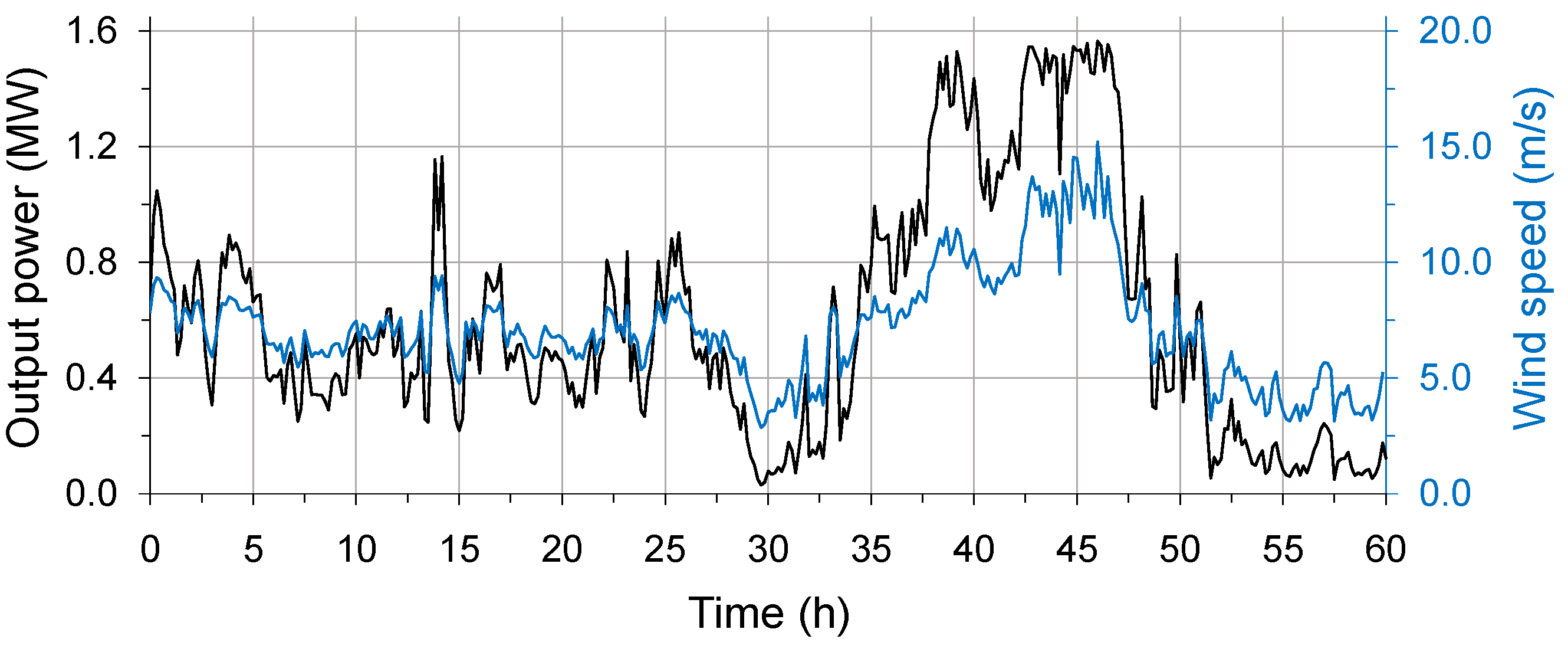
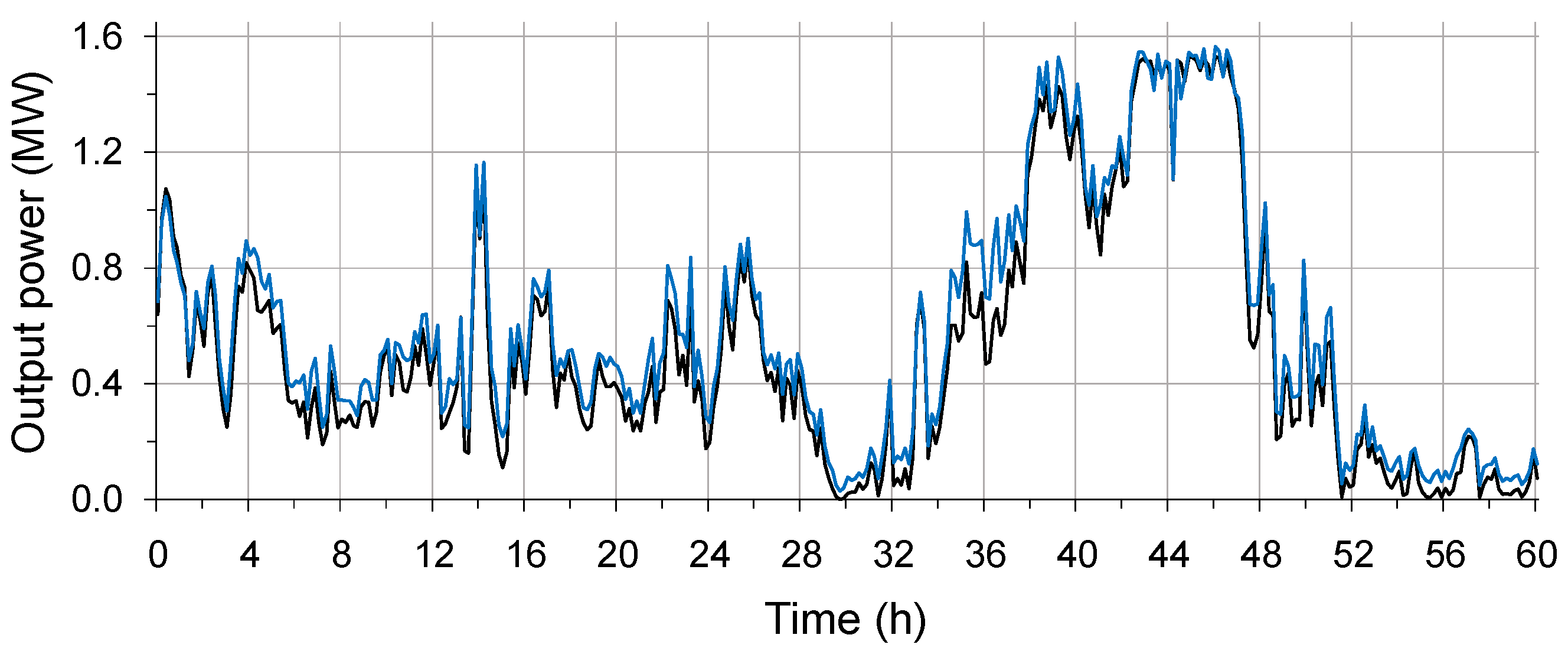
The obtained results from numerical simulations have to be compared with measurements on real systems in order to validate the underlying model and assess its accuracy. For the validation of the wind-to-power conversion, measured time series of the output power and the corresponding wind speed from an onshore turbine with known specific parameters are required. Such measurements, which can be regarded as the most accurate data for validating a wind power model, are difficult to obtain from wind farm operators, e.g., due to data protection regulations. Through a cooperation with the Institute for Applied Geosciences of the TU Berlin concerning the influence of turbine noise on seismic recordings, measured wind speed and output power data of a single turbine are available for this study. The measurements were carried out on a General Electric GE 1.5sl with 1.5 MW rated power and 100 m hub height between 11 and 14 December 2015. The following diagram (Figure 3) shows the time series of the output power and the corresponding wind speed at hub height.
Furthermore, the developed simulation model includes not only physical algorithms for the wind-to-power conversion but takes into account additional turbine losses (described in Section 2.2) and intra-annual changes of the wind turbines for the determination of the generated electricity. The transformation of the simulated time series from UTC to local time and the appropriate temporal aggregation of the final results are also performed by the wind power model. Thus, the time series from the simulations should be validated with measured time series as well.
Power production data of variable renewables like wind power are only available for larger regions, such as entire countries. Hence, the electricity generation from all wind turbines of the dataset has to be spatially aggregated to compare it with measured feed-in data for the whole of Germany, provided by the internet platform SMARD of the Federal Network Agency (www.smard.de) [27]. From this platform, measured data of the German wind power production were downloaded for the entire year 2016. It should be mentioned that no measurement data were available by SMARD on three different days during this period and, thus, the resulting zero values are not considered for the validation and faded out in the concerning diagram (Figure 9).
3. Model
This section describes our simulation model for the electricity generation from wind turbines and on which physical laws it has been implemented. In general, power production data for energy studies can be determined either with statistical methods, e.g., auto-regressive and Monte Carlo models, or with physical models [11,18]. Unlike statistical models [28], the results of physical models, such as the wind power model presented herein, are based on high-resolution weather data from meteorological measurements or numerical models. Therefore, an advantage of physical models compared to statistical methods is the possibility to provide electricity generation data on a highly resolved spatiotemporal scale.
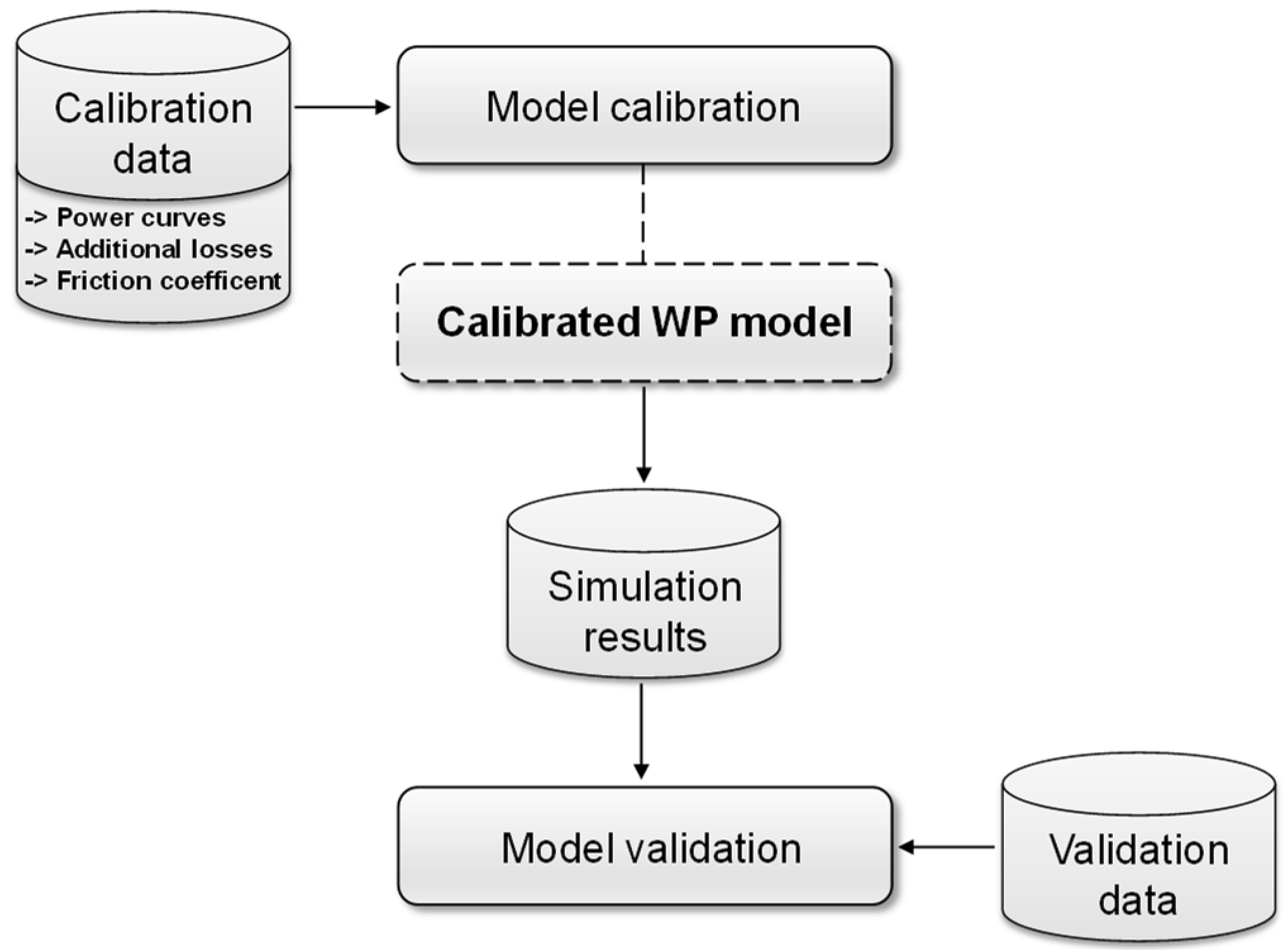
The complete development process from calibration to validation of the wind power model is outlined in Figure 4. In this figure, input and output data are symbolized as containers and the arrows indicate the direction of the data flow.
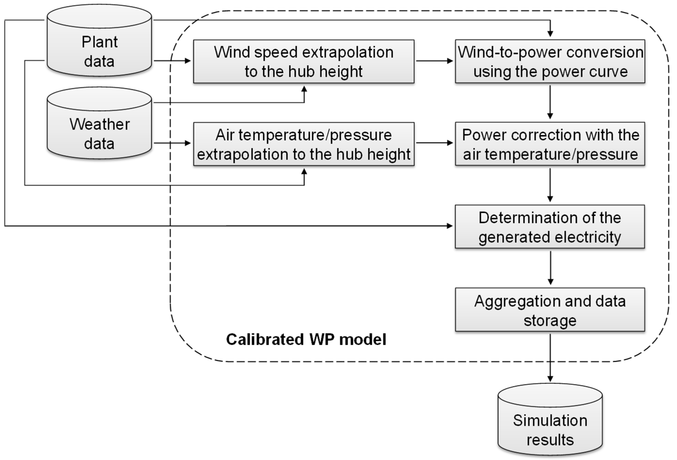
The internal structure of the simulation model is depicted in Figure 5. The plant and weather data in this flowchart represent the input data for the calibrated wind power model. The required calculation steps of the simulation model are displayed as rectangles and all the other symbols have the same meaning as described for Figure 4.
According to Figure 5, the wind power model can be divided into the following main calculation steps, which are performed for each wind turbine of the plant dataset:
- Extrapolation of the weather data provided for the specified plant location to the hub height.
- Wind-to-power conversion with the help of the specific power curve of the wind turbine.
- Correction of the output power using the air temperature and pressure at hub height.
- Calculation of the produced electricity considering additional losses and the date of (de-)commissioning.
- Temporal aggregation of the simulated time series and data storage.
For the extrapolation of the wind speed to the required hub height the Hellmann’s law is applied, which can be expressed by the following relationship:
In Equation (1), v is the unknown wind speed at hub height H and v0 stands for the known wind speed at the height H0, which is 10 m above the ground and obtained from the weather data. The exponent α is called the friction coefficient or Hellmann exponent. This coefficient is a function of the topography at a specific location and frequently assumed as a value of 1/7 for open land [29,30], which corresponds well with the sites of most onshore turbines in Germany. Hence, this value is used for the simulations, but, if necessary and reasonable, other averaged values, e.g., 1/5 or 1/6, can be easily applied in the wind power model. The next step converts the calculated wind speed at hub height to the corresponding output power of the wind turbine. This operation is performed with the help of the power curve, which returns the output power at a standardized air density of 1.225 kg/m3. The main advantage of using the power curve is that no further information about the turbine technology, e.g., the specific rotor diameter or electrical losses of the power generator and converter electronics, has to be known to calculate the output power. Thus, in the presented simulation model, each wind turbine can be treated like a black box with the power curve as its transfer function. The nonlinear section of a typical power curve, as depicted in Figure 6, is typically given by the manufacturer as a table of values. In order to integrate such a nonlinear and discrete relationship into the simulation model with high accuracy and without any additional interpolation routines for intermediate values, the specific power curve is divided into separate sections and these sections are developed to analytical functions. Moreover, to be able to assign the same power curve to similar wind turbines with a different rated power, it is beneficial to use normalized power curves for the wind power model. The specific power curve of most wind turbines, which are often pitch-controlled like the example given in Figure 2, is implemented according to Equation (2). In this relationship, N(v) stands for the normalized output power as a function of the wind speed, i.e., N(v) = P(v)/PR ∈ [0, 1]:
The expression
is a sixth-order polynomial which has to be derived for each power curve used for the numerical simulations. The required coefficients ai of Equation (3) are determined by polynomial regression using the Excel software. It turns out, as shown in Figure 6 for an Enercon E-40, that the development of the nonlinear section of the power curve, i.e., the range between the specific cut-in and rated speed, to a sixth-order polynomial results in precise approximations with coefficients of determination (R2) better than 0.99 and root-mean-square errors (RMSE) lower than 0.01.
For wind turbines with a variable power level above the rated speed, e.g., turbines with a passive stall regulation, the range between the rated and cut-out speed is developed to a sixth-order term by polynomial regression as well. After deriving such analytical representations of the specific power curve, the output power can be calculated straightforwardly for any given wind speed, i.e., without any additional effort for interpolation routines. This calculation step returns the output power PN at a fixed air density of 1.225 kg/m3, which corresponds to an ambient temperature of 288.15 K (15 °C) at normal atmospheric pressure of 1.013 bar. Hence, the obtained power value has to be corrected with the air temperature and pressure at hub height. For this, the ambient temperature provided by the weather data is extrapolated according to the general rule given in [31]:
In this relationship, T describes the air temperature in K at hub height H and T0 stands for the ambient temperature at height H0, which is 2 m above ground level. After estimating the air temperature at hub height, assuming an average temperature gradient over all weather conditions of 0.0065 K/m [31], the output power can be corrected by the following expression derived from the barometric height formula and the power curve correction according to [32]:
In Equation (5), which also considers an exponential reduction of the air pressure with the total height, P stands for the corrected output power at the air temperature and pressure at hub height. The total height HT is given by the sum of the hub height and the ground elevation above sea level, and the so-called scale height has a value of about 8430 m at an isothermal temperature of 288.15 K. Since changes in atmospheric pressure caused by the weather are not considered in these calculations, due to the lack of highly resolved air pressure data in PVGIS, this correction of the output power takes only into account the air temperature at hub height and the air pressure as a function of the total height.
After the correction of the output power, the next calculation step of the wind power model is to determine the generated electricity by multiplying the output power by the given time slot, which is defined by the temporal resolution of the used weather product mostly offering an hourly resolution. This step also includes additional losses of wind turbines, which cannot be covered by calculations based on the power curve, and the date of (de-)commissioning in order to consider intra-annual plant changes. Finally, the resulting hourly resolved time series is transformed from UTC to local time and, if required, converted into an additional time series, e.g., with daily resolution. After the described steps are performed for each wind turbine of the dataset, the time series of the entire plant ensemble are stored as comma-separated values for subsequent processing, e.g., applying a geographical information system (GIS) or a web-based GIS application.
4. Results
The following subsections present the performed simulations using the previously described input data and the wind power model.
4.1. Simulation of a Single Wind Turbine
For proof of concept and model validation, the output power of a wind turbine with known specific parameters is simulated and, afterwards, compared with a measured feed-in time series of this plant. The measurements were performed on a General Electric GE 1.5sl with 1.5 MW rated power and 100 m hub height located in Zodel near the town of Görlitz. As introduced in Section 2.4, the output power and wind speed were measured every 10 min over a period of 60 h (Figure 3). For the calibration of the wind power model, the power curve of this turbine, as shown in Figure 7, is developed into a sixth-order polynomial and implemented with its characteristic parameters, e.g., the specific cut-in and rated speed.
Moreover, the value for additional turbine losses and the Hellmann exponent were set to zero for this simulation, since the wind speed was directly measured at hub height. The ground elevation and ambient temperature required for the calculations were retrieved for this turbine site via PVGIS using the CMSAF weather database. The following diagram (Figure 8) shows the simulated and measured time series of the output power from this single turbine.
As depicted in Figure 8, the wind power model reproduces the pattern of the measured time series very well over the whole period. The frequent underestimation of the simulation results is mainly caused by the fact that the model uses the guaranteed power curve of the General Electric GE 1.5sl from the manufacturer, which may often be exceeded under real conditions. The RMSE of the 10 min data over the complete period, as a statistical measure for such deviations, reaches a value of 84.8 kW. Despite the existing deviations, the introduced wind power model leads to realistic results with a sufficient accuracy. In addition, a Pearson correlation between the first differences of the simulated and measured time series shows a strong positive linear relationship with a correlation coefficient (R-value) of 0.96, indicating that the value pattern of the two time series vary in the same direction and magnitude. Hence, this simulation model can be used to determine the output power and the corresponding electricity production from wind turbines.
4.2. Simulation of the Plant Ensemble
Given the lack of freely accessible electricity production data of wind turbines with a high spatiotemporal resolution, which was the chief motivation for the wind power model presented in this study, it is not possible to benchmark the performance of the whole turbine ensemble on a spatially resolved scale. However, if the simulation results are spatially aggregated over Germany, they can be compared with a publicly available feed-in time series from all German onshore turbines, provided by SMARD [27].
In this subsection, the wind power model was used to determine the electricity generation from 25,835 wind turbines in Germany for the year 2016. For these simulations, each wind turbine of the plant ensemble is calculated individually and the required weather and ground elevation data are retrieved via the PVGIS web interface for each turbine site, using its geographical position. Since the turbine type is often not given in the plant dataset, due to missing information from official sources [8], the turbines are assigned to different power classes with typical power curves. These power classes with the corresponding ranges and the applied turbine types are shown in Table 2. For example, for wind turbines with a rated power in the range between 0.25 and 0.75 MW, the normalized power curve of an Enercon E-40 with a rated power of 0.5 MW was used in the simulation model.
Nevertheless, the plant location, rated power, hub height and the date of (de-)commissioning were considered individually for each turbine. For additional turbine losses, e.g., caused by the effects described in Section 2.2, an overall value of 16% was used for the entire plant ensemble. This value, which typically ranges from 5 to 30% for onshore wind projects according to [33], has been proven by many simulations to be a reasonable average for the considered turbine ensemble.
After carrying out the numerical simulations for 25,835 wind turbines, the hourly resolved data of the plant ensemble were aggregated into a time series to compare the simulation results with measured power generation data of onshore turbines for all of Germany. The simulated and measured time series, which were converted into daily resolutions for a better comparability, are shown in Figure 9.
It can be seen from Figure 9 that the simulated electricity production follows the measured feed-in data well throughout the year. The deviations are mainly caused by the following effects, which are not covered by the wind power model:
- Deviations through the Hellmann’s exponential law with wind speeds at 10 m.
- The uncertainties of the weather data and the fact of hourly averaged values.
- Weather-related changes in air pressure are not considered in the model.
- The assignment of wind turbines to the corresponding power classes.
Nevertheless, with an RMSE of 45.6 GWh determined for the daily resolved data, the obtained results show a good agreement with the measured feed-in time series. In comparison to the annual power generation of 64.0 TWh, produced from all onshore turbines in Germany for the year 2016 according to SMARD, the RMSE shows a value of 0.07%. In addition, a Pearson correlation between the first differences of both time series results in an R-value of 0.97, indicating that the trends of the time series vary in the same direction and magnitude. There are further statistical methods to compare two time series more in-depth, e.g., by applying autoregressive (AR) or autoregressive-moving average (ARMA) models to the time series. Since the similarity of the simulated and measured time series is visually obvious, such models were not performed for this study. In the near future, when the German Core Energy Market Data Register, which also contains the specific turbine types, is fully completed, it will be possible to assign the exact power curve to each wind turbine of the plant dataset. This circumstance should improve the accuracy of the simulation results further.
5. Discussion
The main objective of this study was to generate high-resolution electricity production data of onshore turbines in Germany for a longer period, e.g., an entire year, using publicly available data. For this, the year 2016 was chosen because the applied plant and weather data were only available until the end of 2016 at the writing of this paper. A further reason for this year was the continuation of the energy transition maps of 2015 [4] with power generation data of wind turbines in Germany for 2016. For these energy transition maps, a spatial resolution at LAU2 level is needed. Hence, the introduced simulation model in combination with the CMSAF weather database in PVGIS [25], which provides a high spatial resolution, is well suited for the generation of such maps. The freely available web tool of renewables.ninja (www.renewables.ninja) [34], which also provides electricity generation data of wind turbines for a certain region and period, only applies MERRA-2 weather data with a lower resolution of about 50 km [22], which is not sufficient for the level of detail required for the energy transition maps of 2016.
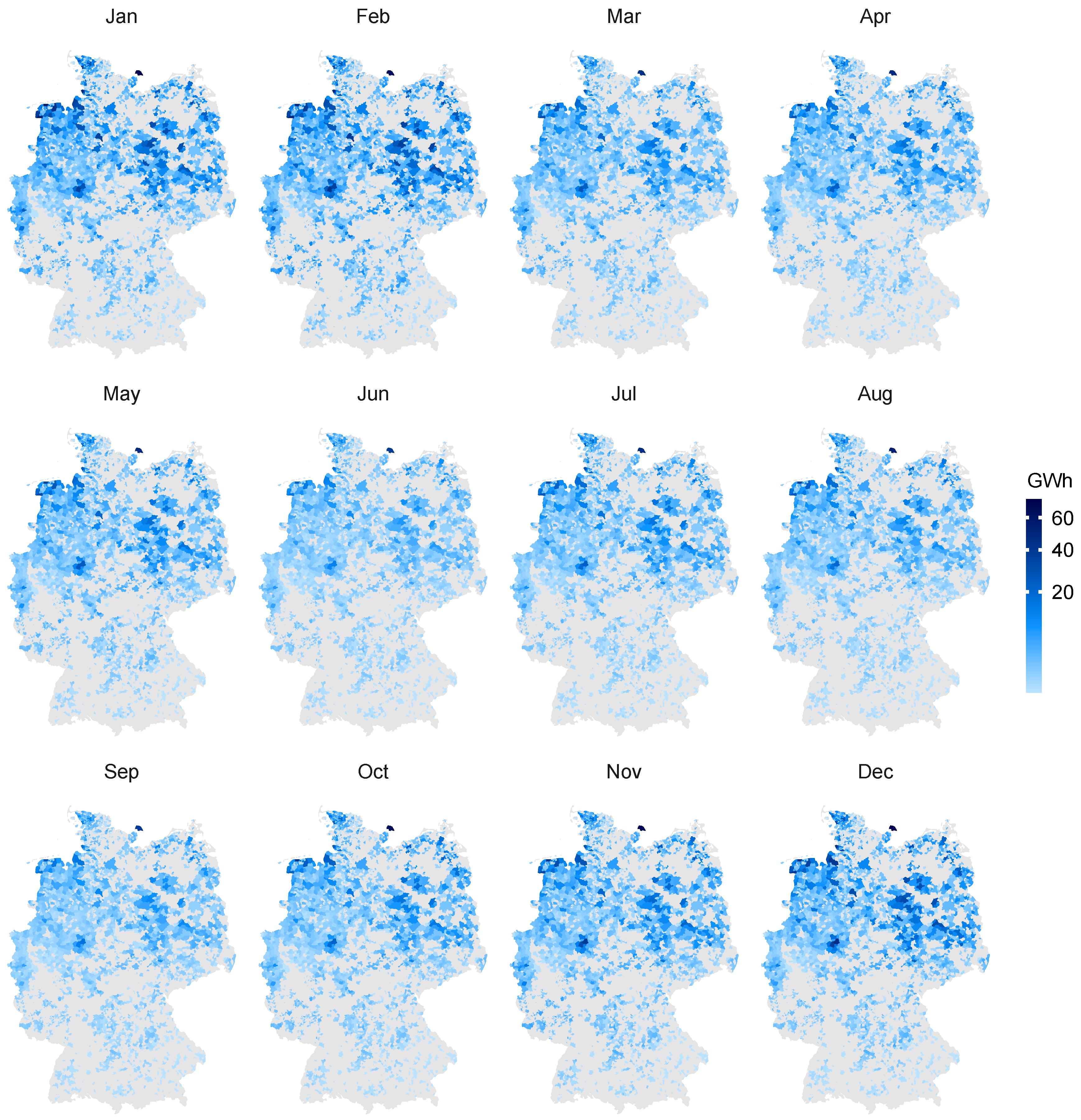
Understanding the variable power generation of existing onshore turbines on a spatiotemporal scale is a precondition for the successful integration of future renewable power plants into increasingly decentralized power systems. Figure 10 shows, as a first utilization example regarding this topic, the monthly electricity production from wind turbines at the spatial resolution of LAU2 based on the performed simulations. Hence, regional advances of the energy transition towards higher shares of wind power can be reliably monitored with the help of such maps.
Moreover, these simulation results can be used in combination with the existing values of the installed capacity, as shown in Figure 1, to determine spatiotemporal capacity factors of onshore turbines in order to investigate their efficiency depending on the specified region and period. For wind turbines, a spatiotemporal capacity factor CFst can be calculated according to Equation (6):
In this expression, T stands for the specified period of time, Cwt is the wind turbine capacity installed in the considered region, and Ewt is the produced electricity from wind turbines in this region and period. Figure 11 shows the monthly capacity factors at the spatial resolution of LAU2 in Germany for the year 2016.
From this figure, it can be easily deduced that the determined capacity factors of wind turbines were much higher from November till February than in the remaining months of 2016. In February, the spatiotemporal capacity factors reached averaged values above 30% almost nation-wide, with a peak value of 64% in Stedesdorf near the town of Wittmund, which also had the annual peak of 72% in January. It is also noteworthy that the northern part of Germany, especially the coastal regions, have the highest capacity factors during the entire year. In June till September, the lowest monthly capacity factors can be found for Germany with averaged values around 10%.
From the numerical simulations in Section 4, it could be clearly seen that, with the help of the developed wind power model, sufficiently precise results can be achieved both for a single wind turbine and a large plant ensemble. For the German wind power production in 2016, 25,835 onshore turbines were taken into account in the simulations in which the power generation of each wind turbine was calculated individually. The obtained results reach a spatial resolution on turbine site level and have an hourly time resolution. To the best of our knowledge, such highly resolved power production data of wind turbines considering almost all onshore plants in Germany [2], which receive guaranteed power feed-in prices according to the EEG, has never been shown before. Furthermore, a new approach was used for the simulation model, in which the nonlinear sections of the specific power curve of a wind turbine are developed into sixth-order polynomials, to simplify and improve the numerical simulations.
6. Conclusions
This paper has shown new ideas for generating high-resolution power production data of onshore turbines in Germany applying a physical model. It was also an objective of this publication to develop a wind power model, in which the focus was set on a very transparent, easy to imitate, and sufficiently precise model approach. To contribute to such an approach, the plant and weather data required for the numerical simulations should be publicly available to give potential users the opportunity to create their own model based on the introduced ideas. It was clearly shown in this study that the developed wind power model can be a promising alternative to obtain highly resolved power generation data of wind turbines using publicly available plant and weather data.
Thus, based on the presented model approach and applying an open-source programming language, such as R or Python, it is possible to generate spatiotemporal power production data of onshore turbines for all of Germany. Such spatiotemporally resolved time series can also help to investigate the electricity generation from wind turbines during extreme weather events, e.g., long periods of calm wind or extended and severe storms. Furthermore, the developed simulation model can be used for other countries or geographical areas without any changes, if all the needed plant and weather data are available for these regions. Furthermore, other applications, e.g., site assessment studies for future wind farms [35] or the influence of wind turbine noise on seismic recordings [36], can benefit from high-resolution electricity generation data delivered by the presented wind power model.
Author Contributions
Conceptualization, Reinhold Lehneis; Methodology, Reinhold Lehneis and David Manske; Software, Reinhold Lehneis and David Manske; Validation, Reinhold Lehneis; Formal Analysis, Reinhold Lehneis and David Manske; Investigation, Reinhold Lehneis; Resources, David Manske and Reinhold Lehneis; Data Curation, David Manske; Writing—Original Draft Preparation, Reinhold Lehneis; Writing—Review and Editing, Reinhold Lehneis, David Manske, and Daniela Thrän; Visualization, David Manske and Reinhold Lehneis; Supervision, Daniela Thrän; Project Administration, Daniela Thrän; All authors have read and agreed to the published version of the manuscript.
Funding
This research received general funding from the Helmholtz Association of German Research Centres.
Informed Consent Statement
Not applicable.
Acknowledgments
The authors gratefully acknowledge Hortencia Flores Estrella (TU Berlin) for providing measurement data on a wind turbine General Electric GE 1.5sl.
Conflicts of Interest
The authors declare no conflict of interest.
References
- GWEC. Global Wind Report 2019; Global Wind Energy Council: Brussels, Belgium, 2020. [Google Scholar]
- BMWi Zeitreihen zur Entwicklung der erneuerbaren Energien in Deutschland unter Verwendung von Daten der Arbeitsgruppe Erneuerbare Energien-Statistik (AGEE-Stat). Available online: https://www.erneuerbare-energien.de (accessed on 30 July 2020).
- IRENA. Renewable Power Generation Costs in 2019; International Renewable Energy Agency (IRENA): Abu Dhabi, UAE, 2020. [Google Scholar]
- Rauner, S.; Eichhorn, M.; Thrän, D. The Spatial Dimension of the Power System: Investigating Hot Spots of Smart Renewable Power Provision. Appl. Energy 2016, 184, 1038–1050. [Google Scholar] [CrossRef]
- Ramirez Camargo, L.; Gruber, K.; Nitsch, F.; Dorner, W. Hybrid Renewable Energy Systems to Supply Electricity Self-Sufficient Residential Buildings in Central Europe. Energy Procedia 2019, 158, 321–326. [Google Scholar] [CrossRef]
- Ramirez Camargo, L.; Nitsch, F.; Gruber, K.; Valdes, J.; Wuth, J.; Dorner, W. Potential Analysis of Hybrid Renewable Energy Systems for Self-Sufficient Residential Use in Germany and the Czech Republic. Energies 2019, 12, 4185. [Google Scholar] [CrossRef]
- Ottenburger, S.S.; Çakmak, H.K.; Jakob, W.; Blattmann, A.; Trybushnyi, D.; Raskob, W.; Kühnapfel, U.; Hagenmeyer, V. A Novel Optimization Method for Urban Resilient and Fair Power Distribution Preventing Critical Network States. Int. J. Crit. Infrastruct. Prot. 2020, 29, 100354. [Google Scholar] [CrossRef]
- Lehneis, R.; Manske, D.; Schinkel, B.; Thrän, D. Modeling of the Power Generation from Wind Turbines with High Spatial and Temporal Resolution. EGU Gen. Assem. Conf. Abstr. 2020. [Google Scholar] [CrossRef]
- Thrän, D.; Bunzel, K.; Klenke, R.; Koblenz, B.; Lorenz, C.; Majer, S.; Manske, D.; Massmann, E.; Oehmichen, G.; Peters, W.; et al. Naturschutzfachliches Monitoring des Ausbaus der Erneuerbaren Energien im Strombereich und Entwicklung von Instrumenten zur Verminderung der Beeinträchtigung von Natur und Landschaft; Bundesamt für Naturschutz: Bonn, Germany, 2020. [Google Scholar]
- Eichhorn, M.; Scheftelowitz, M.; Reichmuth, M.; Lorenz, C.; Louca, K.; Schiffler, A.; Keuneke, R.; Bauschmann, M.; Ponitka, J.; Manske, D.; et al. Spatial Distribution of Wind Turbines, Photovoltaic Field Systems, Bioenergy, and River Hydro Power Plants in Germany. Data 2019, 4, 29. [Google Scholar] [CrossRef]
- Olauson, J.; Bergkvist, M. Modelling the Swedish Wind Power Production Using MERRA Reanalysis Data. Renew. Energy 2015, 76, 717–725. [Google Scholar] [CrossRef]
- Engelhorn, T.; Müsgens, F. How to Estimate Wind-Turbine Infeed with Incomplete Stock Data: A General Framework with an Application to Turbine-Specific Market Values in Germany. Energy Econ. 2018, 72, 542–557. [Google Scholar] [CrossRef]
- Becker, R.; Thrän, D. Completion of Wind Turbine Data Sets for Wind Integration Studies Applying Random Forests and K-Nearest Neighbors. Appl. Energy 2017, 208, 252–262. [Google Scholar] [CrossRef]
- Federal Network Agency Core Energy Market Data Register. Available online: https://www.bundesnetzagentur.de/EN (accessed on 30 July 2020).
- Pierrot, M. The Wind Power. Available online: https://www.thewindpower.net/ (accessed on 25 June 2020).
- Datasheet ENERCON E-40/5.40. ENERCON GmbH, Dreekamp 5, 26605 Aurich (Germany). 2003. Available online: https://www.enercon.de (accessed on 19 May 2020).
- Staffell, I.; Pfenninger, S. Using Bias-Corrected Reanalysis to Simulate Current and Future Wind Power Output. Energy 2016, 114, 1224–1239. [Google Scholar] [CrossRef]
- Olauson, J. ERA5: The New Champion of Wind Power Modelling? Renew. Energy 2018, 126, 322–331. [Google Scholar] [CrossRef]
- González-Aparicio, I.; Monforti, F.; Volker, P.; Zucker, A.; Careri, F.; Huld, T.; Badger, J. Simulating European Wind Power Generation Applying Statistical Downscaling to Reanalysis Data. Appl. Energy 2017, 199, 155–168. [Google Scholar] [CrossRef]
- Bosch, J.; Staffell, I.; Hawkes, A.D. Temporally-Explicit and Spatially-Resolved Global Onshore Wind Energy Potentials. Energy 2017, 131, 207–217. [Google Scholar] [CrossRef]
- Rienecker, M.M.; Suarez, M.J.; Gelaro, R.; Todling, R.; Bacmeister, J.; Liu, E.; Bosilovich, M.G.; Schubert, S.D.; Takacs, L.; Kim, G.-K.; et al. MERRA: NASA’s Modern-Era Retrospective Analysis for Research and Applications. J. Clim. 2011, 24, 3624–3648. [Google Scholar] [CrossRef]
- Gelaro, R.; McCarty, W.; Suárez, M.J.; Todling, R.; Molod, A.; Takacs, L.; Randles, C.A.; Darmenov, A.; Bosilovich, M.G.; Reichle, R.; et al. The Modern-Era Retrospective Analysis for Research and Applications, Version 2 (MERRA-2). J. Clim. 2017, 30, 5419–5454. [Google Scholar] [CrossRef]
- Bollmeyer, C.; Keller, J.D.; Ohlwein, C.; Wahl, S.; Crewell, S.; Friederichs, P.; Hense, A.; Keune, J.; Kneifel, S.; Pscheidt, I.; et al. Towards a High-Resolution Regional Reanalysis for the European CORDEX Domain. Q. J. R. Meteorol. Soc. 2015, 141, 1–15. [Google Scholar] [CrossRef]
- Satellite Application Facility on Climate Monitoring (CM SAF). Available online: https://www.cmsaf.eu/EN/Home/home_node.html (accessed on 18 March 2020).
- EU Science Hub—Photovoltaic Geographical Information System (PVGIS). Available online: https://ec.europa.eu/jrc/en/pvgis (accessed on 25 June 2020).
- Lehneis, R.; Manske, D.; Thrän, D. Generation of Spatiotemporally Resolved Power Production Data of PV Systems in Germany. ISPRS Int. J. Geo Inform. 2020, 9, 621. [Google Scholar] [CrossRef]
- SMARD—Strommarktdaten, Stromhandel und Stromerzeugung in Deutschland. Available online: https://www.smard.de/home/ (accessed on 18 March 2020).
- Ekström, J.; Koivisto, M.; Mellin, I.; Millar, R.J.; Lehtonen, M. A Statistical Modeling Methodology for Long-Term Wind Generation and Power Ramp Simulations in New Generation Locations. Energies 2018, 11, 2442. [Google Scholar] [CrossRef]
- Bañuelos-Ruedas, F.; Angeles-Camacho, C.; Rios-Marcuello, S. Methodologies Used in the Extrapolation of Wind Speed Data at Different Heights and Its Impact in the Wind Energy Resource Assessment in a Region. In Wind Farm—Technical Regulations, Potential Estimation and Siting Assessment; BoD–Books on Demand: Norderstedt, Germany, 2011. [Google Scholar] [CrossRef]
- Petersen, E.L.; Mortensen, N.G.; Landberg, L.; Højstrup, J.; Frank, H.P. Wind Power Meteorology. Part I: Climate and Turbulence. Wind Energy 1998, 1, 2–22. [Google Scholar] [CrossRef]
- Witterung und Klima: Eine Einführung in die Meteorologie und Klimatologie, 11th ed.; Hupfer, P.; Kuttler, W. (Eds.) Vieweg+Teubner Verlag: Wiesbaden, Germany, 2005; ISBN 978-3-322-96749-7. [Google Scholar]
- DIN EN 61400-12-1 VDE 0127-12-1:2017-12 Windenergieanlagen. Available online: https://www.beuth.de/de/norm/din-en-61400-12-1/279191705 (accessed on 5 March 2020).
- Krebs, H.; Kuntzsch, J. Betriebserfahrungen mit Windkraftanlagen auf komplexen Binnenlandstandorten. Erneuerbare Energ. 2000, 12, 2000. [Google Scholar]
- Pfenninger, S.; Staffell, I. Renewables.Ninja. Available online: https://www.renewables.ninja/ (accessed on 29 September 2020).
- Becker, R.; Thrän, D. Optimal Siting of Wind Farms in Wind Energy Dominated Power Systems. Energies 2018, 11, 978. [Google Scholar] [CrossRef]
- Estrella, H.F.; Korn, M.; Alberts, K. Analysis of the Influence of Wind Turbine Noise on Seismic Recordings at Two Wind Parks in Germany. J. Geosci. Environ. Prot. 2017, 5, 76–91. [Google Scholar] [CrossRef]
Figure 1.
(a) Installed wind turbine capacity and (b) intra-annual capacity increase at LAU2 level in Germany for 2016. In the grey areas no wind turbines are (a) installed or (b) have been added during this year.
Figure 1.
(a) Installed wind turbine capacity and (b) intra-annual capacity increase at LAU2 level in Germany for 2016. In the grey areas no wind turbines are (a) installed or (b) have been added during this year.

Figure 2.
Typical power curve (blue line) of a wind turbine using the example of an Enercon E-40 with 0.5 MW rated power. The black dots on the power curve mark the discrete values as given in the manufacturer’s datasheet [16]. The depicted characteristic parameters of the power curve are explained in the following text.

Figure 3.
Measured output power (black line) and wind speed (blue line) time series of a wind turbine General Electric GE 1.5sl located in Zodel near the town of Görlitz. The depicted measurements are performed every 10 min over a period of 60 h.
Figure 3.
Measured output power (black line) and wind speed (blue line) time series of a wind turbine General Electric GE 1.5sl located in Zodel near the town of Görlitz. The depicted measurements are performed every 10 min over a period of 60 h.

Figure 4.
Scheme of the development process of the wind power (WP) model.

Figure 5.
Structure of the WP model shown as a flowchart.

Figure 6.
Approximation of the nonlinear section of the normalized power curve of an Enercon E-40 to a sixth-order polynomial (blue line) with the corresponding coefficient of determination (R2) and root-mean-square error (RMSE). The black dots on the blue line mark the normalized values determined from the discrete values shown in Figure 2 and given in the manufacturer’s datasheet [16].

Figure 7.
Required section of the guaranteed power curve (blue line) of the General Electric GE 1.5sl, which is given by the discrete values (black dots on the blue line) taken from the turbine database of The Wind Power [15].
Figure 7.
Required section of the guaranteed power curve (blue line) of the General Electric GE 1.5sl, which is given by the discrete values (black dots on the blue line) taken from the turbine database of The Wind Power [15].

Figure 8.
Simulated (black line) and measured (blue line) output power of the wind turbine General Electric GE 1.5sl over a period of 60 h with a temporal resolution of 10 min.
Figure 8.
Simulated (black line) and measured (blue line) output power of the wind turbine General Electric GE 1.5sl over a period of 60 h with a temporal resolution of 10 min.

Figure 9.
Simulated electricity production (black line) and measured feed-in data (blue line) from wind turbines in Germany for 2016 with a daily resolution.
Figure 9.
Simulated electricity production (black line) and measured feed-in data (blue line) from wind turbines in Germany for 2016 with a daily resolution.

Figure 10.
Aggregated monthly electricity production from onshore turbines at LAU2 level in Germany for 2016. In the grey areas no wind turbines are installed.
Figure 10.
Aggregated monthly electricity production from onshore turbines at LAU2 level in Germany for 2016. In the grey areas no wind turbines are installed.

Figure 11.
Determined monthly capacity factors of wind turbines at LAU2 level in Germany for 2016. In the grey areas no wind turbines are installed.
Figure 11.
Determined monthly capacity factors of wind turbines at LAU2 level in Germany for 2016. In the grey areas no wind turbines are installed.


Table 1.
Parameters of the turbine dataset used for the wind power model.
| Parameter | Usage |
|---|---|
| Latitude | required |
| Longitude | required |
| LAU-Id 1 | optional |
| Rated power | required |
| Hub height | required |
| Turbine type | optional |
| Commission date | required |
| Decommission date | optional |
1 The LAU-Id is an eight-digit identifier which determines a municipal area or local administrative unit (LAU).
Table 2.
Power classes with the corresponding ranges of rated power (PR) and the applied turbine types.
Table 2.
Power classes with the corresponding ranges of rated power (PR) and the applied turbine types.
| Power Class (MW) | Power Range (MW) | Turbine Type |
|---|---|---|
| 0.1 | PR ≤ 0.15 | Fuhrländer FL100 |
| 0.2 | 0.15 < PR ≤ 0.25 | Enercon E-30 |
| 0.5 | 0.25 < PR ≤ 0.75 | Enercon E-40 |
| 1 | 0.75 < PR ≤ 1.50 | Vestas V52 |
| 2 | 1.50 < PR ≤ 2.50 | Enercon E-82 |
| 3 | 2.50 < PR ≤ 3.50 | Vestas V112 |
| 5 | PR > 3.50 | Enercon E-126 |
Publisher’s Note: MDPI stays neutral with regard to jurisdictional claims in published maps and institutional affiliations. |
© 2021 by the authors. Licensee MDPI, Basel, Switzerland. This article is an open access article distributed under the terms and conditions of the Creative Commons Attribution (CC BY) license (http://creativecommons.org/licenses/by/4.0/).
Share and Cite
MDPI and ACS Style
Lehneis, R.; Manske, D.; Thrän, D. Modeling of the German Wind Power Production with High Spatiotemporal Resolution. ISPRS Int. J. Geo-Inf. 2021, 10, 104. https://0-doi-org.brum.beds.ac.uk/10.3390/ijgi10020104
AMA Style
Lehneis R, Manske D, Thrän D. Modeling of the German Wind Power Production with High Spatiotemporal Resolution. ISPRS International Journal of Geo-Information. 2021; 10(2):104. https://0-doi-org.brum.beds.ac.uk/10.3390/ijgi10020104
Chicago/Turabian StyleLehneis, Reinhold, David Manske, and Daniela Thrän. 2021. "Modeling of the German Wind Power Production with High Spatiotemporal Resolution" ISPRS International Journal of Geo-Information 10, no. 2: 104. https://0-doi-org.brum.beds.ac.uk/10.3390/ijgi10020104
Note that from the first issue of 2016, this journal uses article numbers instead of page numbers. See further details here.