
An Experimental Study of a New Keypoint Matching Algorithm for Automatic Point Cloud Registration


Geomatics Engineering Department, Civil Engineering Faculty, Istanbul Technical University, 34469 Maslak, Istanbul, Turkey
*
Author to whom correspondence should be addressed.
ISPRS Int. J. Geo-Inf. 2021, 10(4), 204; https://0-doi-org.brum.beds.ac.uk/10.3390/ijgi10040204
Submission received: 28 December 2020
/
Revised: 15 March 2021
/
Accepted: 23 March 2021
/
Published: 31 March 2021
(This article belongs to the Special Issue Advanced Research Based on Multi-Dimensional Point Cloud Analysis)
Abstract
:Light detection and ranging (LiDAR) data systems mounted on a moving or stationary platform provide 3D point cloud data for various purposes. In applications where the interested area or object needs to be measured twice or more with a shift, precise registration of the obtained point clouds is crucial for generating a healthy model with the combination of the overlapped point clouds. Automatic registration of the point clouds in the common coordinate system using the iterative closest point (ICP) algorithm or its variants is one of the frequently applied methods in the literature, and a number of studies focus on improving the registration process algorithms for achieving better results. This study proposed and tested a different approach for automatic keypoint detecting and matching in coarse registration of the point clouds before fine registration using the ICP algorithm. In the suggested algorithm, the keypoints were matched considering their geometrical relations expressed by means of the angles and distances among them. Hence, contributing the quality improvement of the 3D model obtained through the fine registration process, which is carried out using the ICP method, was our aim. The performance of the new algorithm was assessed using the root mean square error (RMSE) of the 3D transformation in the rough alignment stage as well as a-prior and a-posterior RMSE values of the ICP algorithm. The new algorithm was also compared with the point feature histogram (PFH) descriptor and matching algorithm, accompanying two commonly used detectors. In result of the comparisons, the superiorities and disadvantages of the suggested algorithm were discussed. The measurements for the datasets employed in the experiments were carried out using scanned data of a 6 cm × 6 cm × 10 cm Aristotle sculpture in the laboratory environment, and a building facade in the outdoor as well as using the publically available Stanford bunny sculpture data. In each case study, the proposed algorithm provided satisfying performance with superior accuracy and less iteration number in the ICP process compared to the other coarse registration methods. From the point clouds where coarse registration has been made with the proposed method, the fine registration accuracies in terms of RMSE values with ICP iterations are calculated as ~0.29 cm for Aristotle and Stanford bunny sculptures, ~2.0 cm for the building facade, respectively.
1. Introduction
Utilizing 3-dimensional (3D) models in various applications considerably increased in this century with the advances in laser scanning technologies [1]. The measurement devices equipped with LiDAR (Light Detection and Ranging) sensors are commonly used for the acquisition of 3D point clouds data, and the developed algorithms for processing the point cloud data provide successful results in generating as-built models to compare with the actual objects. The scanning process for generating accurate 3D point cloud data of different scale objects and/or land-parts is rather fast and practical compared to the conventional photogrammetric and surveying techniques [2]. The measurement with laser scanners bases on the line-of-sight principle, and in most of the cases, the scanned object is acquired partially with overlapping for 3D modeling purposes. Generating a full 3D model from the described modality is contingent on the effective integration of partially obtained data with their alignment relative to a common reference frame. This process is known as the registration of the point cloud data in photogrammetry and computer vision disciplines [1,3]. Beside the density and position accuracy of the point cloud spots, the used approach for the registration process has an essential role in the quality of the final 3D model [2].
In the literature, a number of registration methods have been proposed. In these methods, registration of 3D point clouds obtained from different positions and sensors generally consists of two stages including coarse and fine registration phases [4]. For achieving better results, the fine registration should be applied after the coarse registration by using an appropriate computation algorithm. The iterative closest point (ICP) algorithm and/or its variants has become almost a standard procedure and commonly applied for fine registration in most of the applications [5,6]. Besides, the deep-learning-based fine registration methods such as PointNetLK [7] have also been studied recently. Habib and Alruzouq [8] emphasize four essential points in a comprehensive registration procedure as follows: (i) estimating transformation parameters (that relates the reference frames of the involved point clouds); (ii) defining registration primitives (the conjugate features that should be identified among the used point cloud datasets and used for estimating the transformation parameters); (iii) deciding the similarity measure (the mathematical constraint for describing the coincidence of conjugate features); (iv) deciding an appropriate matching strategy (representing the controlling framework for the automatic registration process) [1]. The initial alignment (coarse registration) methods, which are necessary to apply prior to fine registration process, have been concentrated and studied with growing interest in recent years. Among these methods, the automatic coarse registration algorithms without artificial targets are more demanding [9]. The proposed method in this study is for automatic coarse registration of the point clouds, which are obtained using either the same or different laser scanner devices. In particular, coarse registration methods basically consist of two main steps, namely the detection of the keypoints or the primitives (lines, planes, surfaces) and the description of the conjugates [10].
The keypoint detection and matching tasks in coarse registration require special attention for the derivation of the transformation function precisely. The first step of any matching procedure is to detect the feature locations in the dense point cloud datasets and describe them. In the detection process, the keypoints are defined from the point cloud according to the features such as intensity, surface normal, curvature, red-green-blue (RGB) values, roughness, etc. Hence, once the descriptors are generated, they can be compared to figure out the relationship between the point clouds for carrying out the ‘matching’ procedure in the next step. Therefore, we need a feature detector and descriptor to extract the keypoints in the point clouds accordingly [11].
The working principle of feature detectors and descriptors relies on detecting the keypoints that are covariant to a class of transformations. Then, for each detected feature point, an invariant feature vector representation, called the descriptor, for point cloud spots around the detected keypoint is determined. The feature descriptors can be constituted using the second-order derivatives, parametric equations with estimated coefficients from transforms, or with their combinations [11]. Basically, the extracted features can be categorized as global and local. Global features such as color, texture, etc. are generally considered when an image is concerned in the processes and aim to describe an image as a whole that can be interpreted as a particular property of the image involving all pixels. Considering global color and texture features gives applicable results while looking for similar images in a database. On the other hand, local features are for detecting keypoints either in an image or a point cloud and describing them. In this manner, if the used local feature descriptor reveals n keypoints in the dataset, this means there are n vectors describing each keypoint’s position, orientation, color, etc. Choosing either of the features depends on the purpose of the application; however, local feature descriptors are superior for keypoint matching and point cloud registration purposes [11].
In the literature, there are different algorithms, which are designed and used for keypoint detection, description and matching purposes in point cloud registration [4]. Because the significant contribution of the proposed algorithm in this study is on the coarse registration process, the literature on the coarse registration methods is widely cited here. Basically, coarse registration methods consist of two main steps: the detection step, which includes the determination of either keypoints, lines, planes, surfaces or global features of point clouds; and the description step where the conjugates are determined [10,12]. In the literature, four-points congruent sets (4PCS) and many variants of it are used as a point-based coarse registration algorithm [13]. The 4PCS approach is an algorithm that reduces the number of selected keypoints and simultaneously applies descriptor and matching to determine the conjugate points [12]. Besides, for determining the geometric features of the keypoints in a point-based registration, the descriptors such as point feature histogram (PFH), fast PFH [14], signature of histogram of orientations (SHOT) [15] or the semantic analysis [16,17] methods are commonly used [12]. In the detection step, there are various point-based detectors released so far [18]. Förstner operator [19], 3D Harris [20], local surface patches (LSPs) [21], normal aligned radial feature (NARF) [22], 3D scale invariant feature transform (3DSIFT) [23,24] and intrinsic shape signatures (ISS) algorithm [25] are commonly used as keypoint detectors.
On the other hand, primitive-based registration approaches are also commonly applied for coarse registration, and these approaches include algorithms, which use lines [26], curves [27], planes [9], or surfaces [28]. The global feature-based registration methods including the normal distributions transform (NDT) based algorithms [29] as well as the algorithms that transform 3D point clouds into 1D histograms and 2D images [30] are also among the frequently used algorithms in practice. In this article, a point-based coarse registration approach is proposed and tested.
In this study, a new automatic keypoint description and matching method for coarse registration of point clouds has been introduced and tested. The original contribution of the proposed algorithm is mainly in its descriptor and matching parts. In the description part of the proposed algorithm, the keypoints are divided into subsets using the mathematical combination method. The distances between the reference keypoint and saliency points in the subset and the angles between the constituted connection lines are calculated in a combinational manner. Using the combination technique for constituting the subsets of the keypoints and method used for calculating the distances and angles between the points and lines is the novelty of the proposed algorithm. Contrary the other methods, which are commonly in use in literature, the proposed method considers the calculated angles independently from the surface normal or surface. In the matching algorithm of the new approach, the sum of the differences of the distances and the angle values created for a certain keypoint set in the two-point clouds are taken into account. For matching the subsets, the summations of the differences of the distances and of the angles, respectively, are used as the single values. The set of points whose summation of the distance and angular differences are closest to zero value are considered conjugate points. In addition to descriptor and matching algorithms of the new method, its detector algorithm contains novelty as well. Unlike the ISS and LSP methods, in the proposed detector, a single point with the highest curvature from each voxel (cube) is selected, and the most suitable keypoints are determined accordingly.
The developed automatic new keypoint matching approach for coarse registration was assessed in result of fine registration using the ICP algorithm [5]. The 3D similarity transformation method was employed in the algorithm. The tests of the study have been carried out using three datasets. The first dataset was obtained through the laser scanning measurements in a laboratory environment, and it is to model a small size sculpture. The second dataset included the point clouds of a building facade with regular geometrical details that were obtained through the terrestrial laser scanning measurements from the stationary and mobile platforms. Further information regarding the measurements and the used laser scanning sensors was provided in the second section of the article. Besides the two datasets obtained through the laser scanning by the authors, the tests were repeated using the publicly available bunny point cloud by the Stanford 3D scanning repository (http://graphics.stanford.edu/data/3Dscanrep/ accessed on 15 March 2021) to make the accuracy values obtained with the proposed algorithm reproducible.
The new algorithm, which was suggested for coarse registration in this study, filters the point cloud and down samples the dataset at first. Then, it identifies the keypoints considering the angles and distances among the point cloud spots. The transformation parameters are automatically calculated for the coarse registration with the Gauss Markov least-squares adjustment (LSA) model. After all, fine registration is applied with the ICP method. In order to provide a comparison between the new keypoint descriptor and matching algorithm and the other methods, which are currently in use, the registration processes using both sculptures and building facade data were repeated. Accordingly, ISS and LSP algorithms for keypoint detection and point future histograms (PFH) for keypoint description and matching were used as well. In the conclusions, the tested algorithms were compared by means of accuracy of the transformation before and after ICP as well as the success of the generated 3D models with each algorithm. The new algorithm outperformed the other tested algorithms by providing smaller RMSE values of the transformation and a smaller iteration number in the ICP process.
The organization of this paper is as follows: detailed information of the laser scanning measurements and used datasets were described in Section 2. The theoretical background of the tested keypoint detecting and matching algorithms as well as the new suggested formula were explained in subtitles of this section as well. The mathematical formulation and fundamental theory of the ICP algorithm were summarized in the last subtitle of Section 2. The numerical results with the comparative test statistics were provided in Section 3. A comprehensive discussion based on the obtained results was given in Section 4. Finally, the major conclusions as well as the recommendations for future studies are included in Section 5.
2. Materials and Methods
2.1. Datasets Used in the Tests
In the tests of the point cloud registration algorithms, three datasets were used. The first dataset was obtained with the indoor measurements of Aristotle sculpture (approximate size: 6 cm × 6 cm × 10 cm) (see Figure 1) in ITU Geomatics Engineering Department Surveying Laboratory. NextEngine 3D Laser Scanner Ultra HD was used in the scanning of the sculpture [31]. The dimensional accuracy of the scanner is 0.1 mm in macro mode, and 0.3 mm in wide mode [31]. Considering the size and accuracy of the used laser scanner, it is practical and cost-effective equipment for scanning in 3D model generation of small areas or object in industrial applications.
The point cloud data obtained with scanning the southern facade of ITU Yilmaz Akdoruk guest-house building in Maslak Campus area (Figure 2a) is the second dataset in the study. The facades of the building were scanned using static terrestrial (TLS) and mobile laser scanning (MLS) techniques and the 3D models of the facades were generated by combining the point clouds data obtained from these two techniques. In TLS measurements, Leica ScanStation C10 terrestrial laser scanners with 4 mm distance measurement accuracy, 12″ angle measurement accuracy and 6 mm point position accuracy (for single measurement), was used [32]. Riegl VMX 450 mobile laser scanning system (see Figure 2b) was used for MLS measurements of the building facades [33]. In Riegl VMX-450 mobile laser scanning systems, two Riegl VQ-450 laser scanners with 8 mm position accuracy are integrated with IMU/GNSS unit.
The third dataset used for testing the proposed algorithm is the bunny sculpture point clouds made available by the Stanford 3D scanning repository (http://graphics.stanford.edu/data/3Dscanrep/, accessed on 15 March 2021). The bunny data is known as one of the Stanford models, which was scanned with a Cyberware 3030 MS scanner at Stanford University Computer Graphics Laboratory (see Figure 3). Cyberware 3030 MS scanner has 0.1 mm dimensional accuracy. This data is frequently used as sample model for testing keypoint matching algorithms in literature.
2.2. Methodology
2.2.1. Keypoint Detection
The essential step in the beginning of 3D modeling workflow is the registration of the point clouds data of partially scanned objects. This process requires successfully merging the overlapped point clouds using the estimated transformation parameters. In precise estimation of the transformation parameters, and hence in high performance of point clouds registration, detecting and matching the keypoints rigorously is crucial.
In order to give comparative results on the performance of the detection algorithm suggested and tested in this study, the local surface patches (LSP) and intrinsic shape signatures (ISS) algorithms were also chosen and applied for the keypoint detection. The LSP algorithm is one of the point-wise saliency measurement method, and detects saliency of a vertex considering the shape index (), which bases on the maximum and minimum principle curvatures (, ) at the vertex as given in Equation (1) [21,34].
and if the mean shape index is as given in Equation (2):
where means the set of points in the support of , and is a member of this set, is the number of points in the support of .
Accordingly, a feature point goes out of the pruning steps when its is significantly greater or smaller than such as in , and and are scalar parameters, which define the magnitude of differences from the mean assumed as significant [34].
The intrinsic shape signatures (ISS) algorithm bases on the eigenvalue decomposition of the scatter matrix having the points, which belong to the support of is given in Equation (3) [25]:
where shows the scatter matrix of the support of point , and its eigenvalues with order of decreasing magnitudes are , , . In the process, the points having the ratio between the two successive eigenvalues below a threshold value () are retained (see in Equation (4)).
Further explanations and details of the special cases on the implementation of the ISS algorithm with case studies are given by Tombari et al. [34].
In the proposed and tested detection algorithm given here, similar processing steps with the LSP and ISS point-wise saliency measurement methods are followed, and the surface curvatures at the points are considered in order to identify the keypoints. While estimating the surface curvature at each point, the covariance analysis method, which uses the ratio between minimum and summation of the Eigen values, was preferred. However, while the given algorithms work directly on the point cloud without any intermediate tessellation, the detector concentrates on samples in regions of high curvature and employs the estimates of local variations and quadric error metrics [35]. In the algorithm, a voxel-based filtering is applied to enhance the computational efficiency considering maximum surface curvatures. Accordingly, the point cloud spots, in xyz-plane, are partitioned into three dimensional blocks with an appropriate block size decided considering the resolution of dataset. In each block, the laser spots are further organized into an octree partition structure with a set of three-dimensional voxels (as seen in Figure 4) [36]. Figure 5 gives an overview of the major steps of the suggested keypoint detection algorithm. The keypoint detection algorithm was developed on the Matlab platform.
2.2.2. Keypoint Description and Matching
After extracting the keypoints from point clouds using 3D detectors, which analyze local neighborhoods in order to identify the points of interest as described in the previous section, the neighborhood of a keypoint is described with a 3D descriptor that projects the neighborhood into a proper space. In the end, descriptors defined on different surfaces are matched each other [34]. According to this process, the 3D keypoint descriptors serve a description of the environment in the neighborhood of a point within the cloud, and this description usually depends on the geometrical relationships. Points in two different point clouds having similar feature descriptor mostly correspond to the same surface point.
Principal component analysis (PCA) based keypoint descriptors and matching algorithms are commonly used in various applications including object recognition such as removing roof details of 3D building models. For example, Yoshimura et al. [4] applied the principal component analysis (PCA) efficiently for determining the roof corners and sharp roof lines of the buildings. The PCA technique allows analyzing the saliencies according to the geometric properties of the objects. In their study, Yoshimura et al. [4] considered that the points of a wall and the roof fringes extend along a straight line and hence fit the equation of a straight line (). Thus, they determined the building boundaries considering the lines, which belong to the orthogonal projections of the detected points and matched according to the building edge length and the angle similarity among the issued points.
The point feature histograms (PFH) are also commonly used tools as descriptors [37]. In addition to point matching, the PFH descriptor is also used to determine points in a point cloud, such as points on an edge, corner, and plane. This algorithm uses a Darboux frame (see Figure 6) that is constructed between all point pairs within the local neighborhood of a point [14,38]. The source points of the Darboux frame are the points with the smaller angles between the surface normal and the connecting line of the point pairs and . If is the corresponding point normal, the Darboux frame u, , are constructed as given in Equations (5)–(7):
Three angular distances , and , computed based on the Darboux frame are in Equations (8)–(10):
where is the distance between and (Equation (11)). Three angles and a distance element in addition to two normal vectors are used to describe the geometrical relationship of the point pairs in PFH method. These four elements including the angles and the distance are added to the histogram of the point and the mean percentage of the point pairs in the neighborhood of , which have like relationships. In PFH, these histograms are calculated for all possible point pairs in the k number of neighborhoods of the point [37].
As a different approach, in the four-points congruent sets (4PCS) algorithm, four points are selected from the reference point cloud and their correspondences are searched in the complementing point cloud. Thus the corresponding points are found according to the defined similarity relations (see Figure 7) [39]. In Figure 7, the point e in the reference point cloud (I1) that is selected with intersecting the coplanar connection lines of two-point pairs (a-b and c-d). The corresponding point of e is e′ in the complementing point cloud (I2) in the figure. In Equations (12) and (13), the and ratios are expressed based on the coplanarity of the intersection points and the correspondences of these ratios are sought in the complementing point cloud as well.
The processing with 4PCS algorithm is basically completed in four steps including the following: (i) selecting four points from the point cloud (I1) with considering an adopted threshold, (ii) calculating two intersecting diagonal lengths ( and , as seen in Figure 7); (iii) estimating probable intersection point of two diagonal elements for each point sets. This step is carried out following the expressions given in Equations (14) and (15):
and the difference of these values are compared with a certain threshold as in Equation (16):
and finally, step (iv) determining the most suitable four points, which satisfy the comparison criteria in Equation (16).
In the proposed descriptor and matching algorithm, the cosines of the angles and the Euclidean distances among the connecting lines are considered. Thus, the cosine similarities and the distance equalities of the 3D vectors are taken into account for matching the keypoints (Equation (17)). In the PFH method, three angles connected to the surface normal are used, while (n-2) angles between the connecting lines are calculated for n key points in the proposed method. However, in order to find the geometric similarities of the keypoint sets in the two-point clouds, the differences’ summation of the angle values calculated between the keypoints in both point clouds is taken into account (see Figure 8). As it is seen in Equation (17), the suggested algorithm is based on the use of scalar products of the vectors that is another difference of the new tested algorithm than the commonly used PFH algorithm that uses both cross and scalar products. While the 4PCS method does not use any angle value, it only uses point distance ratio values. In the algorithm proposed here, the (n-1) Euclidean distances are calculated for the n keypoints. For the geometric similarity of the keypoints of the point clouds, the differences’ summation of the distances between the keypoints is taken into account.
In the proposed algorithm, angle cosines are described with Equation (17), and in the equation and are the distance vectors between the salient point and the two other keypoints in the combination subset, is the angle between two distance vectors. In the algorithm, firstly the Euclidean distances among the points in the combination subset and the relevant angle cosines are calculated, and then the similarity of the constructed geometries for each selected salient point sets are considered. Algorithm 1 gives the pseudo-codes of the new keypoint descriptor.
| Algorithm 1. Generation of point cloud features. |
| Input: A point cloud is , number of the sub-points that are going to be selected from the point cloud is . Output: Point cloud feature matrix . 1: 2: 3: 4: 5: for each point combination set in do 6: each point in do 7: 8: 9: 10: 11: 12: 13: end for 14: end for 15: return |
The notations used in the algorithm are as follows: is feature matrix for the descriptor (a null matrix in the beginning), is the total number of the keypoints in the point cloud “”. is the matrix, which holds all possible subsets of the point combinations, and is the number of the identified keypoints in the subsets. The means “reference point”, and is benchmark. The is the function for calculating the angle cosines and is the function for calculating the Euclidean distances among the feature points.
According to this algorithm, firstly, the total number of points in the keypoint list is determined with an identification number (as ID = 1 to that is the total number of points). This ID information is used as the labels of the points in the performed operations. Then, using the labels of the points, possible subsets () consisting of elements among the all points are generated. Generating the subsets is a basic combination process in the algorithm and is expressed in the line 3 of the pseudocodes (see Algorithm 1).
In result of the described process, each salient point in a subset having elements is considered as a reference point () and the remaining points in the subset are taken as the benchmarks (), and the process is repeated iteratively. Hence the angle and distance values ( and ) are calculated and subsequently written into a separate row of the matrix belong to the addressed point ID information. The given part of the process so far (as given between the lines 7 and 11 in Algorithm 1) runs only the descriptor part of the registration and allows us defining the distinctive features, which are required for matching, and base on the described geometry with the angular and distance relations among the potential keypoints.
In the proposed algorithm, the descriptor part includes calculating the Euclidean distances between all points and the angles between all vectors in the subset. Figure 9 illustrates the calculation of the cosine similarity in algorithm. According to this illustration, if we consider the subset having four points, one point is accepted as a reference at each iteration and this assumption generates two angle cosines and three distance elements between the reference and the benchmarks. These numbers of parameters in algorithm can be generalized as (n-2) angle cosines and (n-1) distance elements when the number of the points in the subset is shown with n. The points identified as keypoints in result of iterative process of similarity checks constitute the matrix elements.
Following the identification process, the keypoints are available to be matched. Algorithm 2 gives the pseudocodes of the applied matching process. In the algorithm, the subpoint sets are selected from the source and target point clouds in order to match the keypoints between the two-point clouds. Accordingly, , , and are the input parameters in the algorithm. and are the source and target point clouds, respectively. is the number of points in the subsets that are selected from each point cloud in each iteration. These parameters are also included in Algorithm 1 with the same symbols. is a threshold parameter for deciding the angle-based geometrical similarities. In the output of the algorithm, the information of the matched point sets selected from the source and target point clouds showing highest similarity are included in a matrix with the name of in the algorithm.
In Algorithm 2, the properties of point subsets, which are determined by using Algorithm 1 for the source (indicated with indices S) and target (indicated with indices T) point clouds, are calculated. This process is seen in lines 1 and 2 of the algorithm, and the calculated properties are expressed with and that include the outputs of Algorithm 1. Then, the distances between points and angles between vectors of the keypoint sets in the source point cloud are compared with the same properties of the keypoint sets in the target point cloud. In lines 6 and 7 of Algorithm 2, the similarity checks are coded. In the lines, the variables and are differences between the angle similarity properties and the distance similarity properties, respectively. Then, the ID information ( and ) of the points that the relevant features belong to them, and the similarities calculated from these features are stored in a matrix.
After the and calculations, which are carried out in a certain order following the clock-wise turn, the matrix is organized in order to have rows with descending values. The rows with values smaller than the threshold are selected in the matrix. These selected rows correspond to the points in the subset with the highest similarity in the source (S) and target (T) point clouds. Thereafter, these rows, which are recorded in a matrix, are reordered in order to have descending values, and hence the optimum subset of the points for matching purpose is determined. In summary of the followed process, the points are roughly selected considering the angular similarity and they are ordered with respect to the distance-based similarity. In the final step of our description and matching algorithm, the points having the distance differences close to zero values are selected as the common keypoints of the point clouds.
| Algorithm 2. Selection of the subpoint sets from the source and target point clouds for matching. |
| Input: Source and target point clouds are and , number of the sub-points that are going to be selected from the point cloud is , distance threshold for similarity of angle based features is . Output: Matrix storing the information of matched sub-point sets of and . 1: 2: 3: 4: for each feature vector in feature matrix do 5: for each feature vector in feature matrix do 6: 7: 8: 9: 10: 11: 12: end for 13: end for 14: 15: 16: 17: return |
The processing steps of the descriptor and matching algorithms (see in the pseudocodes given in Algorithms 1 and 2) of the proposed method are also summarized with a flowchart in Figure 10.
2.2.3. Iterative Closest Point (ICP) Algorithm
The iterative closest point algorithm completes the registration of two coarsely aligned point clouds; hence, it aims to provide combined point cloud data in the end of the process. Basically, an ICP algorithm follows these four steps: (i) detecting and selecting keypoints; (ii) matching the points according to minimum distance difference principle; (iii) calculating the rotations R(, , ) and translations T(, , ); (iv) providing an optimum alignment in result of the iterative process [5,41]. Iterations in the algorithm are continued until the root mean square error of the transformation residuals decreases under a predetermined threshold value () or a given iteration number () [5]. Figure 11 shows the ICP algorithm steps.
The iterative closest point (ICP) algorithm can be used with various geometric data including point sets, polylines, implicit and parametric curves, triangulated faceted surfaces. In principle, the ICP algorithm handles these geometrical representations by evaluating the closest points in two datasets. In the formulation of the algorithm, means a “data” (target) shape, which is moved (registered) to be in best alignment with as a “model” (source) shape [5]. The distance “” between an individual data point of and a model is shown in Equation (18).
In the equation, the closest point in that yields the minimum distance is represented by and that . The closest point (from to ) is calculated for each point in [5].
One of the fundamental issues in the ICP algorithm is 3D coordinate transformation. Before the ICP registration, the coarse alignment of the point clouds has involved the coordinate transformation process as well. Therefore, the coarse registration of the point clouds involves the estimation of the 3D Helmert transformation parameters including three translations, three rotation angles and a scale factor, in combining process [42]. As different from transformation process in the coarse alignment, the number of estimated parameters in the ICP fine registration part is only six including translation and rotations. Because the scale factor is estimated in coarse registration once, it is excluded out of estimated parameters in ICP iterations. Depending on the obtained accuracy of the estimated 3D transformation, the registration process is classified as either coarse or fine registration [43]. Coarse registration provides a rough alignment of the point clouds and may be sufficient as depending on the purpose of the study. However, in applications where higher accuracy is required, fine registration is needed, and fining process begins after an initial alignment of the point clouds with coarse registration [44].
The seven-parameters Helmert similarity transformation is commonly applied in registration of the point clouds. The conjugate keypoints, which have been detected, identified and matched for the point clouds (conjugate keypoints for the first and second point clouds , that = 1,2…) in the coarse registration section, are used for estimating seven transformation parameters (, , , , , ). 3D Helmert similarity transformation is formulated as given in Equation (19):
In the equation, the Cartesian coordinates of a conjugate keypoint in the first and second point cloud are (, , ), and (, , ), respectively. The rotation parameters are evaluated in an orthogonal rotation matrix and added to the translation parameters after multiplying with a scale factor () [45].
Seven transformation parameters given in Equation (19) are estimated using known coordinates of at least three conjugate keypoints in both point clouds, and in case of availability of more common keypoints, the transformation parameters can also be calculated with least squares adjustment by adopting the given condition in Equation (20) [46]:
where, is the residual matrix and is the weight matrix of the observables contributed to estimating the parameter in mathematical model of the least squares adjustment procedure.
After estimating the transformation parameters with sufficient accuracy, it will be possible to transform the coordinates of a target point cloud (; = 1,2…) into the source point cloud (; = 1,2…) successfully. In this step, the crucial issue is to determine the transformation parameters as precise as possible. In order to increase the accuracy of the parameters, improving the estimation values step by step iteratively is an effective and generally applied approach.
Other than the conventional ICP method as introduced by Besl and McKay [5], many variants of this algorithm have been developed and used. In these variant formulations, the performance of the original algorithm was tried to be increased by means of accuracy as well as the processor efficiency in computations [47]. Zhang [48] enhanced the conventional ICP technique by replacing the error function with a robust kernel [49]. Chen and Medioni [50] modified the algorithm with replacing the point-to-point distance with the point-to-tangent plane definition [51].
3. Results
3.1. Performance of the Keypoint Detection Algorithms
The case study on testing the proposed detection algorithm that we introduced in this study, were carried out using three different datasets including the building facade, Aristotle and Stanford bunny sculptures’ point clouds. The datasets have been described in Section 2.1. In the proposed detection algorithm, the mean curvature of the surface was calculated. Then, the data was filtered according to the optimum curvature criterion that considers the changes of calculated curvatures at the points. After that, a voxel-based filter was applied (see Figure 12).
The result of filtering the terrestrial laser scanning point cloud data on the building facade can be seen in Figure 12a with the voxels, and the filtering results of the sculptures, which were colored according to the curvature values, are given in Figure 12b for the Aristotle and Figure 12c for the Stanford bunny. At the initial process, filtering the point cloud is one of the crucial steps that is applied prior identifying the corresponding keypoints.
In order to provide comparative results on the keypoint detection routines and a discussion on their role in ICP performance, we applied the intrinsic shape signatures (ISS) and local surface patch (LSP) methods in the numerical tests using all datasets. The theoretical background and formulations of these methods have already been described in Section 2.2.1. In the result of the keypoint detection process using point cloud data of the Aristotle sculpture, the numbers of detected keypoints for each point clouds are ~60 points with the ISS algorithm and ~180 points with the LSP algorithm. Figure 13 visualizes the density and distribution of the detected keypoints with each algorithm. On the other hand, the number of identified keypoints with the new algorithm is 18 for the Aristotle sculpture.
Using the point cloud datasets obtained from the terrestrial laser scanning (TLS) and mobile laser scanning (MLS) measurements for the building facade, the ISS algorithm revealed ~34 keypoints in TLS point cloud data and ~88 keypoints in MLS point cloud data, whereas the LSP algorithm detected ~200 keypoints for each point cloud datasets obtained from TLS and MLS techniques, respectively. Figure 14 shows the distributions of the detected keypoints using the ISS and LSP algorithms from two TLS and MLS point clouds. Using the proposed algorithm, the approximate number of keypoints detected according to the filtering of calculated curvatures in the TLS and MLS point clouds is 30 for the building facade (see Figure 12a and Figure 18).
In the result of keypoint detection process using point cloud data of Stanford bunny sculpture, the numbers of detected keypoints for each point clouds are ~150 points with the ISS algorithm and ~350 points with the LSP algorithm. On the other hand, the number of identified keypoints with proposed algorithm is 14 for the Stanford bunny sculpture (see Figure 12c and Figure 19).
3.2. Performance Tests of Keypoint Descriptor and Matching Algorithms
In the proposed descriptor algorithm, the angle cosine values between the 3D direction vectors are calculated, and the cosine similarities among the conjugate geometries are searched. The significant originality of the registration algorithm, which is introduced and tested in this article, lays behind its description and matching approach. The theoretical details of the description and matching part of the algorithm are explained in Section 2.2.2. In the point cloud data of Aristotle sculpture, five points of 18 keypoints were matched by the description and matching routine of our algorithm. Figure 15 shows the distribution of matched keypoints of the Aristotle sculpture.
In addition to the new algorithm, the keypoints, which were matched according to the keypoint histograms obtained from the PFH descriptor with the help of the ISS and LSP detectors, were also used in the study. In the result of the ISS+PFH process, six points of ~60 identified keypoints were matched for Aristotle sculpture point cloud datasets (Figure 16). Following the LSP+PFH algorithm, eight points of ~180 identified keypoints were matched for Aristotle sculpture modeling (Figure 17).
In the description and matching procedure, which were carried out for building facade using terrestrial (TLS) and mobile (MLS) laser scanning data, automatic process of the algorithms (ISS+PFH, LSP+PFH, the proposed algorithm) did not give successful results to match the conjugate points. This is mainly because of the large discrepancies among the identified keypoints sets in each point clouds, and therefore the failure of establishing similarity relations for matching. Unlike the automatic description and matching process, the semi-automatic way of processing where the saliency points are identified using the criteria formulated in Section 2.2.1, and selected manually according to their convenience for similarity, gave result. In this part of the process with the building facade point clouds, filter and detection procedures were carried out considering mean curvatures at the points using our detection algorithm. Thereafter the identified keypoints as the output of the detection algorithm were fed manually into the proposed description and matching algorithm. Figure 18 shows the conjugate points matched using semi-automatic matching of the keypoints identified with the new detector (Algorithms 1 and 2).
In the point cloud data of the Stanford bunny sculpture, five points of 14 keypoints were matched by the description and matching routine of our algorithm. The second plot of Figure 19 shows the distribution of the matched keypoints of the bunny sculpture. In addition to the new algorithm, the ISS+PFH process was able to match only three points of the detected ~150 keypoints. On the other hand, the LSP+PFH algorithm did not provide any matching among the ~350 identified keypoints.
3.3. Numerical Validations of the Applied Algorithms in Fine Registration with the ICP Method
High accuracy determination of the coordinate transformation parameters between the point clouds is crucial in combining the datasets for generating a seamless model of 3D objects. The initial alignment of the point clouds appropriately with pre-defined transformation parameters in coarse registration phase plays an essential role in the overall performance of the fine registration using ICP. In this study, we applied the Gauss–Markov adjustment method in calculation of the transformation parameters using the similarity relations among the matched points determined in Section 3.2, and we evaluated the results considering the root mean square errors (RMSE) of the transformation and iteration numbers of computational convergence.
In the tests, three case study datasets (including the Aristotle sculpture, building facade, and Stanford bunny sculpture) were used. The numerical validations were carried out employing three different coarse registration algorithms (ISS+PFH, LSP+PFH, the new purposed algorithm). In validations using each dataset, the matched keypoints as the output of each coarse registration algorithm, the fine registrations of the point clouds datasets have been carried out with the iterative closest point (ICP) method. The success of the tested coarse registration algorithms including the proposed one was assessed and compared through the fine registration accuracies by means of the reached RMSE values in ICP iterations. The iteration numbers that the ICP converged were also considered as another measure to assess the contribution of the coarse registration algorithms on the efficiency of the fine registration process.
The first test was carried out using coarsely aligned point clouds with the matched keypoints for the Aristotle sculpture using the ISS+PFH algorithm. Table 1 shows the transformation parameters calculated with six conjugate points identified with the ISS+PFH algorithm and used for the coarse alignment of point clouds. In the same table, the transformation parameters are given for small and big rotation angles among the axes of two coordinate systems, which are subject to transformation. When the two sets of transformation parameters are compared, it is seen that the calculated parameters have higher accuracy, and thus the RMSE value of the transformation is smaller when the rotation angles are bigger.
In Table 1, the RMSE value of the transformation is ; are translation parameters with their RMSE values (in centimeter), and , , are the rotation parameters with their RMSE values (in radian), and s is the scale factor with its accuracy.
Figure 20 summarizes the results obtained from the iterative refining of transformation parameters using ICP for Aristotle sculpture datasets. In the illustrations given in the figure, the point clouds are given before and after transformation processes using final transformation parameters of ICP. As seen from the given graphic below the illustrations, the RMSE value of the ICP converged at 20th iteration, and the accuracy of the ICP iterations dropped from 7.0 cm to 0.9 cm when the keypoints were matched using the ISS+PFH algorithm.
The second test was carried out using coarsely aligned point clouds with the matched keypoints for Aristotle sculpture but this time using LSP+PFH algorithm. Table 2 shows the transformation parameters calculated with eight conjugate points identified with LSP+PFH algorithm and used for the coarse alignment of point clouds. According to given statistics in the table, the transformation parameters calculated for the point clouds having big rotation angles among the coordinate axes have higher accuracy and thus provide relatively more precise transformation.
Figure 21 shows the graphical illustrations of point clouds before and after fine registration with ICP, and the decreasing RMSE values of the transformation with the increased number of iterations in the graphic below the figure. Considering this graphic, it is seen that the RMSE value of the ICP converged in 30th iteration and the accuracy of the transformation decreased from ~6.0 cm to ~1.0 cm using the LSP+PFH matching algorithm. When compared with the ICP results of point clouds, which have been roughly aligned using the ISS+PFH algorithm, the obtained final accuracy in the result of second test is worse, and the convergence of iterations took longer time. In summary, the ICP process after both the ISS+PFH and LSP+PFH gave similar accuracies around ~1.0 cm.
In the last test with Aristotle sculpture data, fine registration of point clouds, which were aligned using the new proposed algorithm, was carried out with the ICP method. Table 3 gives the transformation parameters calculated with five conjugate points identified with the new algorithm and used for the coarse alignment of point clouds. According to given statistics in the table, the accuracy of the transformation between the point clouds using the conjugate points by the new algorithm was higher than the accuracies obtained in previous two tests. Additionally, similar to the previous tests, higher accuracy transformation parameters were obtained with the bigger rotation angles.
In Figure 22, the ICP method performance after the coarse registration with the new algorithm is demonstrated with visual graphics of the point clouds before and after matching. The RMSE value of the ICP converged in 10th iteration, which means a significant improvement in performance of registration algorithm compared to other tested algorithms in previous tests. The accuracy statistic of iterations dropped ~0.29 cm while it was not better than ~0.90 cm for the other algorithms.
The ICP method was applied to the building facade data as well. In the coarse registration process, the TLS and MLS point clouds keypoints and semi-automatically identified conjugate points using the new algorithm were used. In the evaluation of the building facade datasets, the automatic evaluation of the ISS+PFH and LSP+PFH algorithms have not been successfully applied in coarse registration because there were no keypoints successfully matched. Therefore, the keypoints for coarse alignment of the point clouds were identified manually from the saliency points such as window corners (see Figure 18) and introduced to the semi-automatic matching process with the PFH algorithm. However, this trial was also not successful for matching with the PFH algorithm. Different patterns, characteristics and resolutions of two-point clouds data acquired from terrestrial and mobile platforms using different sensors possibly caused this inconsistency, and therefore the automatic and semi-automatic processes were failed in matching the keypoints. The only solution for matching the keypoints of the building facade dataset was applying semi-automatic matching with the new suggested method. In this solution, the keypoints were identified manually from the saliency points, and put into the new matching algorithm.
In Table 4, the transformation parameters between the TLS and MLS point clouds in the coarse registration process using the semi-automatically identified common points using the new algorithm were given. In Figure 23, the ICP method performance for the building facade datasets was shown. According to given graphics, the RMSE value of the ICP converged in 50th iteration, and it dropped ~0.02 m.
The ICP method was also applied using the Stanford bunny dataset as well. Into the process, the coarsely aligned point clouds with five keypoints, which were matched using the new algorithm, were inserted. Table 5 shows the calculated transformation parameters in the result of coarse alignment. In Figure 24, the ICP method performance after the coarse registration with the new algorithm is demonstrated with visual graphics of the bunny point clouds before and after matching. The RMSE value dropped ~0.29 cm at the 15th iteration of the ICP.
Because the LSP+PFH method did not provide any conjugate keypoint in result of matching process using bunny data, the coarse alignment was not possible. The ISS+PFH method output only three conjugate keypoints, which were not evenly distributed on the object. Using coarsely aligned point clouds with three conjugate keypoints by the ISS+PFH method, the ICP algorithm provided an RMSE value of ~0.50 cm at the 15th iteration for bunny dataset.
4. Discussion
We developed and introduced a new method for automatic keypoint detection, description, and matching for 3D point cloud coarse registration in this study. The first part of the new method includes a 3D keypoint detection algorithm, which was formulated based on similar working principles with the ISS and LSP methods. In the second part, a 3D descriptor (Algorithm 1) and 3D keypoints matching algorithms (Algorithm 2) were designed and coded. This second part of the designed algorithm is rather different than its counterparts by means of defining the geometrical configuration among the saliency points according to the differential numerical combinations (see Section 2.2.2.) as well as the computational efficiency; hence, it includes original contribution. In order to compare the new algorithm with commonly used counterparts, we included ISS and LSP detectors with the PFH descriptor routine in the numerical tests. The transformation between the point clouds using the matched points in the algorithms was carried out using the Helmert similarity transformation method. The fine registration part has been carried out using the ICP method as formulated in Section 2.2.3. The validation results of three case studies clarified the superior performance of the new algorithm and its contribution to the fine registration performance with ICP by means of success in combining two-point clouds with higher accuracy registration with a smaller number of iterations.
In the numerical tests using point cloud data obtained from shifted perspectives with ultra HD laser scanning measurements with the same 3D laser scanner for small size sculptures (the Aristotle and Stanford bunny), automatic keypoint detection, description, and matching algorithms worked successfully in coarse registration of the point clouds. However, comparisons of the RMSE values of the transformation in coarse registration proved the superiority of the new algorithm over its tested counterparts (see the test results in Section 2.2.3.). Fine registration with the ICP method followed the coarse registration with the tested detection, description and matching algorithms using the point clouds data of the sculptures. In the tests with the ICP algorithm, the efficiency achieved in the iterative improvement of the registration confirmed the superior performance of the new algorithm in matching the keypoints for automatic registration of the point clouds datasets. With the ICP method, it could be possible to obtain RMSE of ~0.29 cm within a reasonable converging time using the new algorithm, whereas the achievable accuracy with the matched keypoint sets by the ISS+PFH and LSP+PFH was ~1.00 cm for the Aristotle sculpture and ~0.50 cm for the Stanford bunny (only ISS+PFH is available for the bunny) at best in the longer convergence time. This result proved the importance of initial alignment with the coarse registration process for generating improved models from the employed point clouds measured with a shift. In literature, it is possible to find similar research studies on investigating the performance of automatic keypoint detection algorithms and their effects on generation of 3D models. Among these studies, Yew and Lee [52] recently carried out research with the ISS+FPFH and ISS+3DFeat-Net algorithms and found conclusions, which confirm our results, regarding the performance.
Another experiment with the tested algorithms was carried out with the point cloud datasets of a building facade, obtained from the outdoor measurements using two different laser scanners mounted on a stationary tripod on a ground station and a mobile land vehicle. However, automatic description and matching algorithms of the point clouds keypoints with each detector did not give successful results and failed in the registration. An important reason for the failure of automatic registration process is the differences among the resolution and qualities of two-point cloud data because they were obtained using different laser scanners on stationary and mobile platforms. Semi-automatic selection and evaluation of the keypoints from the building facade data compensated the problem. Consequently, matching the keypoints for the transformation in coarse registration was carried out with manually fed keypoints to the semi-automatized algorithm. In ICP tests with building facade data, the initially aligned point clouds using the new algorithm provided applicable results by means of final RMSE value of the ICP (~2.0 cm) within a reasonable converging iteration number, and hence its competence in combining the point clouds obtained by the measurements from different platforms has been proven.
There are strengths and weaknesses of the proposed algorithm in practice. The proposed method provides smaller RMSE values in lower iteration numbers than the ISS+PFH and LSP+PFH algorithms. It provides better performance in the description and in matching the keypoints. Although the number of detected keypoints with the proposed algorithm is even less than the other coarse registration algorithms, fine registration of the point clouds, which were coarsely aligned point clouds with the proposed algorithm, provided smaller RMSE values in the ICP method. This method is superior to the ISS+PFH and LSP+PFH methods especially in the coarse registration of point clouds with different resolutions obtained from different laser scanners.
Because the description and matching algorithm of the proposed method is based on the combination method, and because the distance and angle values are calculated for all point combinations in the subset, large amounts of keypoint combinations are examined, and this makes the description and matching process longer and increases the memory and processor burden in the computer system. The relatively cumbersome and limited capabilities of the platform on which the algorithm computation codes were written create another disadvantage in practice for the proposed method.
The proposed algorithm is based on the point-based process. Especially while working with large datasets, not finding the conjugate points and/or mismatching problems constitutes another disadvantage of the new algorithm. In such cases, semi-automatic operation (with manual selection of the saliency points to be matched) of the algorithm is suggested and provides accurate results.
Regarding the large-scale experiment using the proposed algorithm, the method works semi-automatically. Our proposed algorithm needs to be enhanced in the detection of the keypoints of large-scale datasets if we want to apply it automatically in large-scale experiments. Depending on our experiences, this weakness is also valid for other coarse registration algorithms as well (e.g., ISS+PFH, LSP+PFH).
5. Conclusions
The new algorithm developed and tested in this study is promising for the resultant accuracy of the obtained products as well as the computational efficiency. However, there are still further developments, which are needed to search for especially while combining the point clouds data with changing accuracies and resolutions obtained from different platforms and/or larger areas. Improving the algorithms by employing intelligent techniques having the handling capability of stochastic information of the datasets can lead to the expected improvements in results. In order to aimed progress, in future work, we plan to focus on integrating deep learning features into our algorithms with variance estimation modules. By means of improving computational efficiency and optimization in use of the computer processors, we aim to move the automatic matching algorithm that we designed to another programming platform with parallel processing capability. By developing the automatic keypoint detection and selection algorithm, we plan to expand the research for evaluating the large-scale point cloud datasets.
Author Contributions
Conceptualization, Ramazan Alper Kuçak and Serdar Erol; methodology, Ramazan Alper Kuçak and Serdar Erol; software, Ramazan Alper Kuçak; validation, Serdar Erol and Ramazan Alper Kuçak; Formal Analysis, Serdar Erol and Ramazan Alper Kuçak; investigation, Ramazan Alper Kuçak; resources, Serdar Erol and Ramazan Alper Kuçak; data curation, Ramazan Alper Kuçak, Serdar Erol and Bihter Erol; writing—original draft preparation, Ramazan Alper Kuçak and Bihter Erol; writing-review & editing, Bihter Erol, Ramazan Alper Kuçak and Serdar Erol; visualization, Serdar Erol, Ramazan Alper Kuçak and Bihter Erol; supervision, Serdar Erol; funding acquisition, Serdar Erol and Ramazan AlperKuçak. All authors have read and agreed to the published version of the manuscript.
Funding
This research received no external funding.
Institutional Review Board Statement
Not applicable.
Informed Consent Statement
Not applicable.
Data Availability Statement
Data sharing is not applicable to this article.
Acknowledgments
This research was carried out as part of the first author’s PhD thesis study at Istanbul Technical University, Graduate School of Science Engineering and Technology. Abbas Memiş is acknowledged for the discussions on optimal design and development of program codes for the new algorithm and numerical assessments. Riegl WMX 450 mobile mapping system was provided by Koyuncu 3D Lidar Map and Engineering Company to this study. The point cloud data and keypoints were visualized using CloudCompare Software. Automatic matching algorithms were coded using Matlab Software, and the other algorithms were used from PCL (Point Cloud Library) that was coded in C++ programing language. We are grateful to Jakob Wilm and Martin Kjer of the Danish Technical University for the ICP algorithm used in this study [53]. The Stanford bunny data has been used from the Stanford Computer Graphics Laboratory 3D Scanning Repository.
Conflicts of Interest
The authors declare no conflict of interest.
References
- Fangning, H.; Ayman, H. A closed-form solution for coarse registration of point clouds using linear features. J. Surv. Eng. 2016, 142, 04016006. [Google Scholar] [CrossRef]
- Vosselman, G.; Maas, H.G. Airborne and Terrestrial Laser Scanning; CRC Press: Beacon Raton, FL, USA, 2010; pp. 1–318. [Google Scholar]
- Buenoa, M.; González-Jorgea, H.; Martínez-Sánchezac, J.; Lorenzo, H. Automatic point cloud coarse registration using geometric keypoint descriptors for indoor scenes. Autom. Constr. 2017, 81, 134–148. [Google Scholar] [CrossRef]
- Yoshimura, R.; Date, H.; Kanai, S.; Honma, R.; Oda, K.; Ikeda, T. Automatic registration of MLS point clouds and SfM meshes of urban area. Geo-Spat. Inf. Sci. 2016, 19, 171–181. [Google Scholar] [CrossRef]
- Besl, P.J.; McKay, N.D. Method for registration of 3-D shapes. In Sensor Fusion IV: Control Paradigms and Data Structures; International Society for Optics and Photonics: Bellingham, WA, USA, 1992. [Google Scholar]
- Rusinkiewicz, S.; Levoy, M. Efficient variants of the ICP algorithm. In Proceedings of the Third International Conference on 3-D Digital Imaging and Modeling, Quebec, QC, Canada, 28 May–1 June 2001. [Google Scholar]
- Aoki, Y.; Goforth, H.; Srivatsan, R.A.; Lucey, S. PointNetLK: Robust & efficient point cloud registration using pointnet. In Proceedings of the IEEE/CVF Conference on Computer Vision and Pattern Recognition, Long Beach, CA, USA, 15–20 June 2019; pp. 7163–7172. [Google Scholar]
- Habib, A.F.; Alruzouq, R.I. Line-based modified iterated Hough transform for automatic registration of multi-source imagery. Photogramm. Rec. 2004, 19, 5–21. [Google Scholar] [CrossRef]
- Chen, S.; Nan, L.; Xia, R.; Zhao, J.; Wonka, P. PLADE: A Plane-Based Descriptor for Point Cloud Registration with Small Overlap. IEEE Trans. Geosci. Remote Sens. 2019, 58, 2530–2540. [Google Scholar] [CrossRef]
- Habib, A.; Detchev, I.; Bang, K. A comparative analysis of two approaches for multiple-surface registration of irregular point clouds. Int. Arch. Photogramm. Remote Sens. Spat. Inf. Sci. 2010, 38, 1–6. [Google Scholar]
- Hassaballah, M.; Abdelmgeid, A.A.; Alshazly, H.A. Image features detection, description and matching. In Image Feature Detectors and Descriptors; Awad, A., Hassaballah, M., Eds.; Springer: Cham, Switzerland, 2016; pp. 11–45. [Google Scholar]
- Xu, Y.; Boerner, R.; Yao, W.; Hoegner, L.; Stilla, U. Pairwise coarse registration of point clouds in urban scenes using voxel-based 4-planes congruent sets. ISPRS J. Photogramm. Remote Sens. 2019, 151, 106–123. [Google Scholar] [CrossRef]
- Aiger, D.; Mitra, N.J.; Cohen-Or, D. 4-points congruent sets for robust pairwise surface registration. ACM Trans. Graphics 2008, 27, 1–10. [Google Scholar] [CrossRef] [Green Version]
- Rusu, R.B.; Blodow, N.; Beetz, M. Fast point feature histograms (FPFH) for 3D registration. In Proceedings of the 2009 IEEE International Conference on Robotics and Automation, Kobe, Japan, 12–17 May 2009. [Google Scholar]
- Tombari, F.; Salti, S.; Di Stefano, L. Unique Signatures of Histograms for Local Surface Description. In European Conference on Computer Vision; Daniilidis, K., Maragos, P., Paragios, N., Eds.; Springer: Berlin, Germany, 2010. [Google Scholar]
- Yang, B.; Dong, Z.; Liang, F.; Liu, Y. Automatic registration of large-scale urban scene point clouds based on semantic feature points. ISPRS J. Photogramm. Remote Sens. 2016, 113, 43–58. [Google Scholar] [CrossRef]
- Ge, X. Automatic markerless registration of point clouds with semantic-keypointbased 4-points congruent sets. ISPRS J. Photogramm. Remote Sens. 2017, 130, 344–357. [Google Scholar] [CrossRef] [Green Version]
- Huang, R.; Xu, Y.; Yao, W.; Hoegner, L.; Stilla, U. Robust global registration of point clouds by closed-form solution in the frequency domain. ISPRS J. Photogramm. Remote Sens. 2021, 171, 310–329. [Google Scholar] [CrossRef]
- Förstner, W. A framework for low level feature extraction. In European Conference on Computer Vision; Eklundh, J.O., Ed.; Springer: Berlin, Germany, 1994. [Google Scholar]
- Sipiran, I.; Bustos, B. Harris 3D: A robust extension of the Harris operator for interest point detection on 3D meshes. Vis. Comput. 2011, 27, 963–976. [Google Scholar] [CrossRef]
- Chen, H.; Bhanu, B. 3D free-form object recognition in range images using local surface patches. Pattern Recognit. Lett 2007, 28, 1252–1262. [Google Scholar] [CrossRef]
- Steder, B.; Rusu, R.B.; Konolige, K.; Burgard, W. Point feature extraction on 3D range scans taking into account object boundaries. In Proceedings of the 2011 IEEE International Conference on Robotics and Automation, Shanghai, China, 9–13 May 2011. [Google Scholar]
- Lowe, G. SIFT-the scale invariant feature transform. Int. J. Comput. Vis. 2004, 2, 91–110. [Google Scholar] [CrossRef]
- Rusu, R.B.; Cousins, S. 3D is here: Point cloud library (PCL). In Proceedings of the 2011 IEEE International Conference on Robotics and Automation, Shanghai, China, 9–13 May 2011. [Google Scholar]
- Zhong, Y. Intrinsic shape signatures: A shape descriptor for 3D object recognition. In Proceedings of the 2009 IEEE 12th International Conference on Computer Vision Workshops, ICCV Workshops, Kyoto, Japan, 27 September–4 October 2009. [Google Scholar]
- Habib, A.; Ghanma, M.; Morgan, M.; Al-Ruzouq, R. Photogrammetric and lidar data registration using linear features. Photogram. Eng. Remote Sens. 2005, 71, 699–707. [Google Scholar] [CrossRef]
- Yang, B.; Zang, Y. Automated registration of dense terrestrial laser-scanning point clouds using curves. ISPRS J. Photogram. Remote Sens. 2014, 95, 109–121. [Google Scholar] [CrossRef]
- Ge, X.; Wunderlich, T. Surface-based matching of 3D point clouds with variable coordinates in source and target system. ISPRS J. Photogram. Remote Sens. 2016, 111, 1–12. [Google Scholar] [CrossRef] [Green Version]
- Magnusson, M.; Lilienthal, A.; Duckett, T. Scan registration for autonomous mining vehicles using 3D-NDT. J. Field Robot. 2007, 24, 803–827. [Google Scholar] [CrossRef] [Green Version]
- Huang, R.; Ye, Z.; Boerner, R.; Yao, W.; Xu, Y.; Stilla, U. Fast pairwise coarse registration between point clouds of construction sites using 2D projection based phase correlation. Int. Arch. Photogramm. Remote Sens. Spat. Inf. Sci. 2019, 42, 1015–1020. [Google Scholar] [CrossRef] [Green Version]
- Nextengine-Next Engine 3D Laser Scanner Ultra HD Handbook. Available online: https://www.nextengine.com/assets/pdf/scanner-techspecs-uhd.pdf (accessed on 1 December 2020).
- Leica, Leica ScanStation C10–the All-in-One Laser Scanner for Any Application. Available online: http://w3.leica-geosystems.com/downloads123/hds/hds/scanstationc10/brochures-datasheet/leica_scanstation_c10_ds_en.pdf (accessed on 1 December 2020).
- Riegl, Riegl VMX-450 Compact Mobile Laser Scanning System Data Sheet. Available online: http://www.riegl.com/uploads/tx_pxpriegldownloads/DataSheet_VMX-450_2015-03-19.pdf (accessed on 1 December 2020).
- Tombari, F.; Salti, S.; Di Stefano, L. Performance evaluation of 3D keypoint detectors. Int. J. Comput. Vis. 2013, 102, 198–220. [Google Scholar] [CrossRef]
- Pauly, M.; Gross, M.; Kobbelt, L.P. Efficient simplification of point-sampled surfaces. In Proceedings of the IEEE Visualization. VIS 2002, Boston, MA, USA, 27 October–1 November 2002. [Google Scholar]
- Qin, H.; Guan, G.; Yu, Y.; Zhong, L. A voxel-based filtering algorithm for mobile LiDAR data. Int. Arch. Photogramm. Remote Sens. Spat. Inf. Sci. 2018, 42, 1433–1438. [Google Scholar] [CrossRef] [Green Version]
- Rusu, R.B.; Marton, Z.C.; Blodow, N.; Beetz, M. Persistent point feature histograms for 3D point clouds. In Proceeding of the 10th International Conference International Autonomous Systems (IAS-10), Baden, Germany, 23–25 July 2008; pp. 119–128. [Google Scholar]
- Hänsch, R.; Weber, T.; Hellwich, O. Comparison of 3D interest point detectors and descriptors for point cloud fusion. ISPRS Ann. Photogramm. Remote Sens. Spat. Inf. Sci. 2014, 2, 1–57. [Google Scholar] [CrossRef] [Green Version]
- Novak, D.; Schindler, K. Approximate registration of point clouds with large scale differences. ISPRS Ann. Photogramm. Remote Sens Spat. Inf. Sci. 2013, 1, 211–216. [Google Scholar] [CrossRef] [Green Version]
- Theiler, P.W.; Wegner, J.D.; Schindler, K. Markerless point cloud registration with keypoint-based 4-points congruent sets. ISPRS Ann. Photogramm. Remote Sens. Spat. Inf. Sci. 2013, 1, 283–288. [Google Scholar] [CrossRef] [Green Version]
- Gressin, A.; Mallet, C.; David, N. Improving 3D lidar point cloud registration using optimal neighborhood knowledge. In Proceedings of the ISPRS Annals of the Photogrammetry, Remote Sensing and Spatial Information Sciences, Melbourne, Australia, 25 August–1 September 2012; pp. 111–116. [Google Scholar]
- Al-Durgham, K.; Habib, A. Association-matrix-based sample consensus approach for automated registration of terrestrial laser scans using linear features. Photogramm. Eng. Remote Sens. 2014, 80, 1029–1039. [Google Scholar] [CrossRef]
- Matabosch, C.; Salvi, J.; Fofi, D.; Meriaudeau, F. Range image registration for industrial inspection. In Proceedings of the Machine Vision Applications in Industrial Inspection XIII, International Society for Optics and Photonics, San Jose, CA, USA, 24 February 2005. [Google Scholar]
- Al-Rawabdeh, A.; He, F.; Moussa, A.; El-Sheimy, N.; Habib, A. Using an unmanned aerial vehicle-based digital imaging system to derive a 3D point cloud for landslide scarp recognition. Remote Sens. 2016, 8, 95. [Google Scholar] [CrossRef] [Green Version]
- Watson, G. Computing helmert transformations. J. Comput. Appl. Math. 2006, 197, 387–394. [Google Scholar] [CrossRef] [Green Version]
- Ghilani, C.D. Adjustment Computations: Spatial Data Analysis; John Wiley & Sons: Hoboken, NJ, USA, 2017. [Google Scholar]
- Boukebbab, S.; Gheribi, H.; Linares, J.M. A procedure for total knee alignment prosthesis using the ICP algorithm in the aim to implant it in the biomechanical engineering. Vibroeng. Proc. 2016, 9, 44–49. [Google Scholar]
- Zhang, Z. On local matching of free-form curves. In BMVC92; Hogg, D., Boyle, R., Eds.; Springer: London, UK, 1992; pp. 347–356. [Google Scholar] [CrossRef]
- Press, W.H.; Teukolsky, S.A.; Vetterling, W.T.; Flannery, B.P. Numerical Recipes in C, 2nd ed.; Cambridge University Press: London, UK, 2002; pp. 59–70. [Google Scholar]
- Chen, Y.; Medioni, G. Object modelling by registration of multiple range images. Image Vis. Comput. 1992, 10, 145–155. [Google Scholar] [CrossRef]
- Fitzgibbon, A.W. Robust registration of 2D and 3D point sets. Image Vis. Comput. 2003, 21, 1145–1153. [Google Scholar] [CrossRef]
- Yew, Z.J.; Lee, G.H. 3dfeat-net: Weakly supervised local 3D features for point cloud registration. In Proceedings of the European Conference on Computer Vision, Munich, Germany, 8–14 September 2018. [Google Scholar]
- Kjer, H.M.; Wilm, J. Evaluation of Surface Registration Algorithms for PET Motion Correction. Bachelor′s Thesis, Technical University of Denmark, Lyngby, Denmark, 2010. [Google Scholar]
Figure 1.
Aristotle sculpture at ITU Geomatics Engineering Department Metrology Laboratory.

Figure 2.
(a) ITU Yilmaz Akdoruk guest-house southern facade; (b) point cloud of the building facade and its environment measured by using the mobile laser scanning system (Riegl VMX-450).
Figure 2.
(a) ITU Yilmaz Akdoruk guest-house southern facade; (b) point cloud of the building facade and its environment measured by using the mobile laser scanning system (Riegl VMX-450).

Figure 3.
Bunny sculpture by the Stanford 3D scanning repository (http://graphics.stanford.edu/data/3Dscanrep/, accessed on 15 March 2021).
Figure 3.
Bunny sculpture by the Stanford 3D scanning repository (http://graphics.stanford.edu/data/3Dscanrep/, accessed on 15 March 2021).

Figure 4.
On the building facade: (a) curvatures calculated at the surface points; (b) the surface data partitioned into cubic voxels; (c) the salient points after filtering the point cloud.
Figure 4.
On the building facade: (a) curvatures calculated at the surface points; (b) the surface data partitioned into cubic voxels; (c) the salient points after filtering the point cloud.

Figure 5.
Overview of the major steps of the proposed keypoint detection algorithm.

Figure 6.
Darboux frame between a point pair (adapted from [38]).
Figure 6.
Darboux frame between a point pair (adapted from [38]).

Figure 7.
Principle of point selection in four-points congruent sets (4PCS) algorithm (adapted from [39,40]).

Figure 8.
Cosine similarity algorithm.

Figure 9.
Cosine similarity combination approach.

Figure 10.
The fundamental processing steps of the descriptor and matching algorithms of the proposed algorithm in the study.
Figure 10.
The fundamental processing steps of the descriptor and matching algorithms of the proposed algorithm in the study.

Figure 11.
Iterative closest point (ICP) algorithm steps.

Figure 12.
The fully automatic keypoint detection with the proposed algorithm: (a) for the building facade with voxels, (b) for the Aristotle sculpture and (c) for the Stanford bunny sculpture with color.
Figure 12.
The fully automatic keypoint detection with the proposed algorithm: (a) for the building facade with voxels, (b) for the Aristotle sculpture and (c) for the Stanford bunny sculpture with color.


Figure 13.
Distribution of detected keypoints for the point clouds data of Aristotle sculpture using: (a) intrinsic shape signatures (ISS) algorithm; (b) local surface patch (LSP) algorithm.
Figure 13.
Distribution of detected keypoints for the point clouds data of Aristotle sculpture using: (a) intrinsic shape signatures (ISS) algorithm; (b) local surface patch (LSP) algorithm.

Figure 14.
Distribution of the detected keypoints for point cloud datasets for building facade using the following: (a) intrinsic shape signatures (ISS) algorithm with TLS data; (b) ISS algorithm with MLS data; (c) local surface patch (LSP) algorithm with TLS data; (d) LSP algorithm with MLS data.
Figure 14.
Distribution of the detected keypoints for point cloud datasets for building facade using the following: (a) intrinsic shape signatures (ISS) algorithm with TLS data; (b) ISS algorithm with MLS data; (c) local surface patch (LSP) algorithm with TLS data; (d) LSP algorithm with MLS data.

Figure 15.
Aristotle sculpture: (a) detected keypoints in the 1st point cloud using new algorithm; (b) distribution of the matched keypoints with the new algorithm; (c) detected keypoints in the 2nd point cloud using new algorithm.
Figure 15.
Aristotle sculpture: (a) detected keypoints in the 1st point cloud using new algorithm; (b) distribution of the matched keypoints with the new algorithm; (c) detected keypoints in the 2nd point cloud using new algorithm.

Figure 16.
Aristotle sculpture: (a) the keypoints identified by ISS in the 1st point cloud; (b) matching two-point clouds with the ISS+PFH algorithm; (c) the keypoints identified by ISS in the 2nd point cloud.
Figure 16.
Aristotle sculpture: (a) the keypoints identified by ISS in the 1st point cloud; (b) matching two-point clouds with the ISS+PFH algorithm; (c) the keypoints identified by ISS in the 2nd point cloud.

Figure 17.
Aristotle sculpture: (a) the keypoints identified by LSP in the 1st point cloud; (b) matching two-point clouds with LSP+PFH algorithm; (c) the keypoints identified by LSP in the 2nd point cloud.
Figure 17.
Aristotle sculpture: (a) the keypoints identified by LSP in the 1st point cloud; (b) matching two-point clouds with LSP+PFH algorithm; (c) the keypoints identified by LSP in the 2nd point cloud.

Figure 18.
Building facade: (a) the keypoints identified by the new detector in the TLS point cloud; (b) matching TLS and MLS point clouds using semi-automatic evaluation of the new algorithm; (c) the keypoints identified by the new detector in the MLS point cloud data.
Figure 18.
Building facade: (a) the keypoints identified by the new detector in the TLS point cloud; (b) matching TLS and MLS point clouds using semi-automatic evaluation of the new algorithm; (c) the keypoints identified by the new detector in the MLS point cloud data.

Figure 19.
Stanford bunny sculpture: (a) detected keypoints in the 1st point cloud using new algorithm; (b) distribution of the matched keypoints with the new algorithm; (c) detected keypoints in the 2nd point cloud using new algorithm.
Figure 19.
Stanford bunny sculpture: (a) detected keypoints in the 1st point cloud using new algorithm; (b) distribution of the matched keypoints with the new algorithm; (c) detected keypoints in the 2nd point cloud using new algorithm.

Figure 20.
Aristotle sculpture: results obtained from iterative closest point (ICP) algorithm where the keypoints identified and matched by the ISS+PFH algorithm are used.
Figure 20.
Aristotle sculpture: results obtained from iterative closest point (ICP) algorithm where the keypoints identified and matched by the ISS+PFH algorithm are used.

Figure 21.
Aristotle sculpture: results obtained from the iterative closest point (ICP) algorithm where the keypoints identified and matched by LSP+PFH algorithm are used.
Figure 21.
Aristotle sculpture: results obtained from the iterative closest point (ICP) algorithm where the keypoints identified and matched by LSP+PFH algorithm are used.

Figure 22.
Aristotle sculpture: results obtained from iterative closest point (ICP) algorithm where the keypoints identified and matched by the new algorithm are used.
Figure 22.
Aristotle sculpture: results obtained from iterative closest point (ICP) algorithm where the keypoints identified and matched by the new algorithm are used.

Figure 23.
Building facade: results obtained from iterative closest point (ICP) algorithm where the TLS and MLS point clouds’ keypoints identified and matched by the new algorithm are used.
Figure 23.
Building facade: results obtained from iterative closest point (ICP) algorithm where the TLS and MLS point clouds’ keypoints identified and matched by the new algorithm are used.

Figure 24.
Stanford bunny sculpture: the results obtained from iterative closest point (ICP) algorithm where the keypoints identified and matched by the new algorithm are used.
Figure 24.
Stanford bunny sculpture: the results obtained from iterative closest point (ICP) algorithm where the keypoints identified and matched by the new algorithm are used.


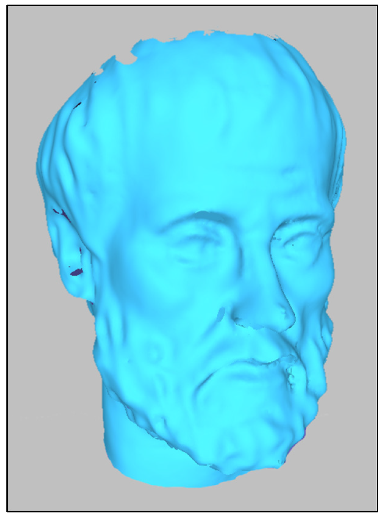
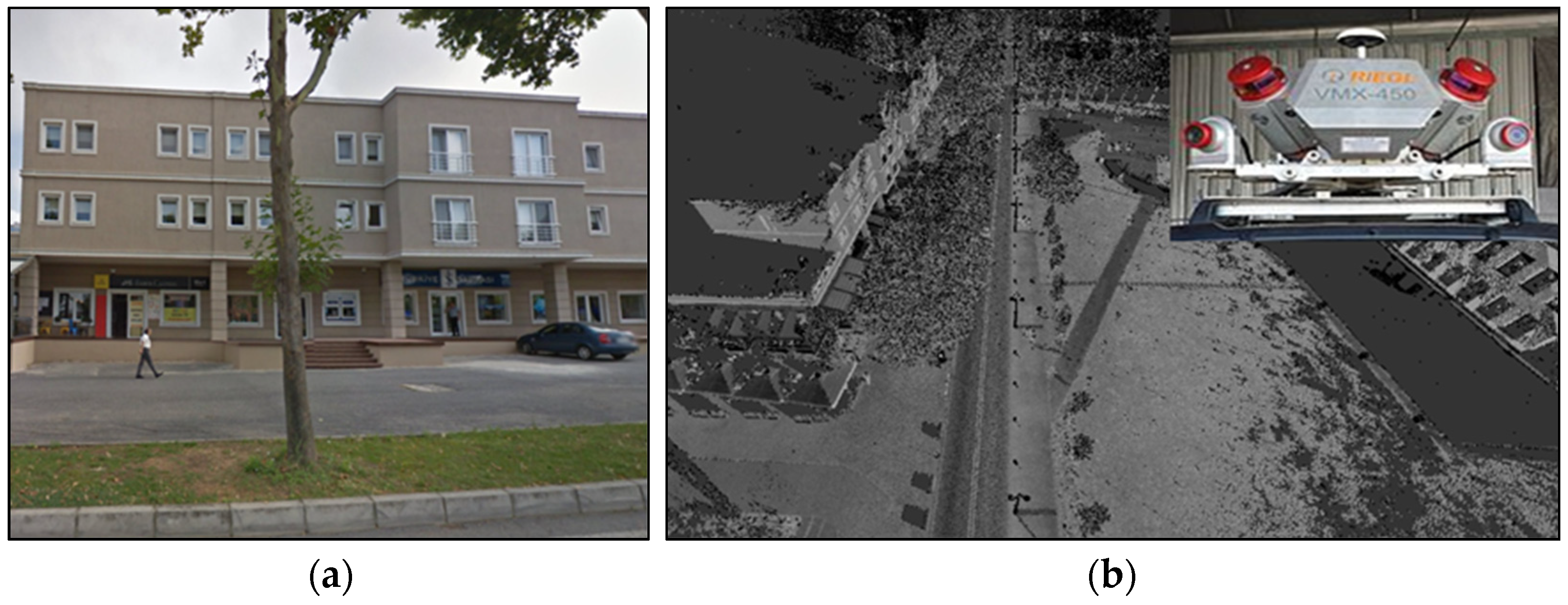
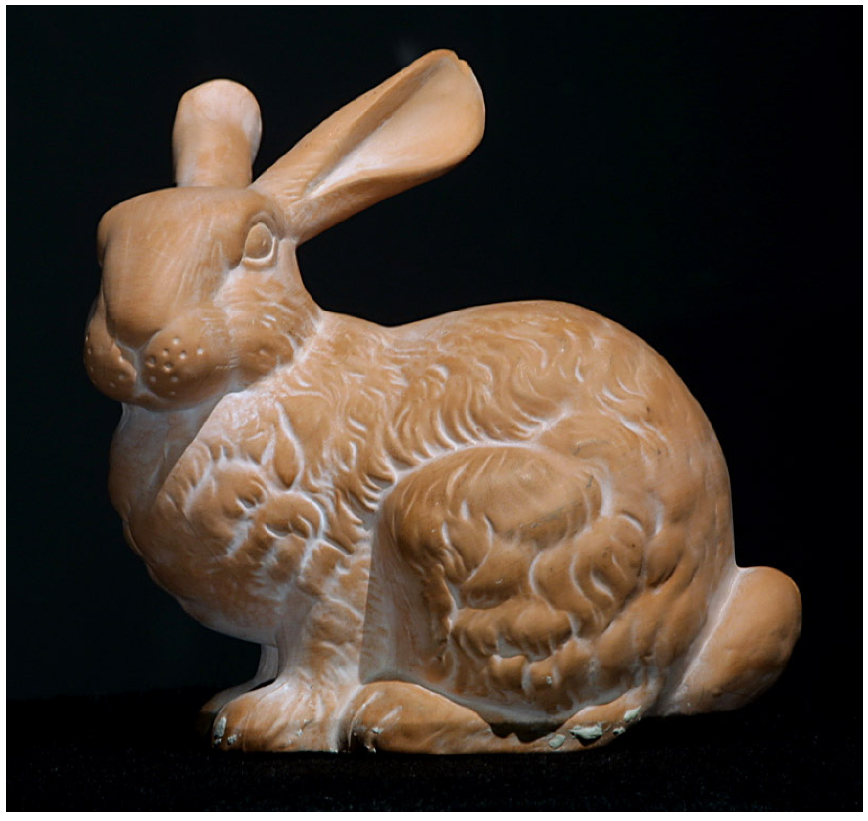
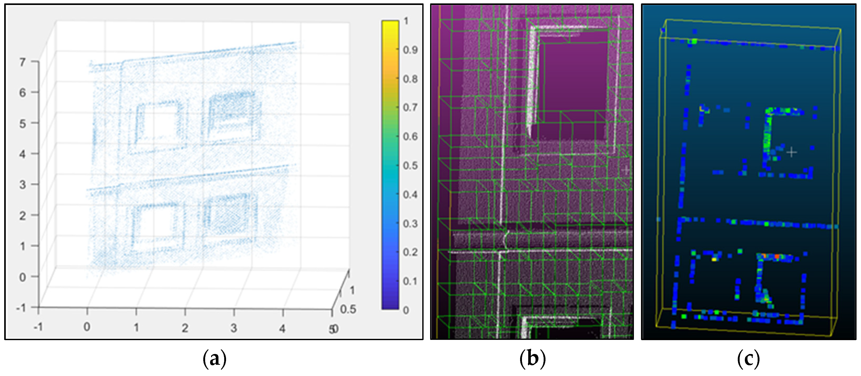
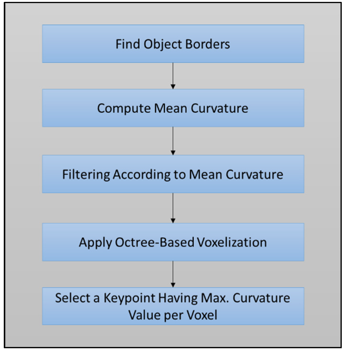
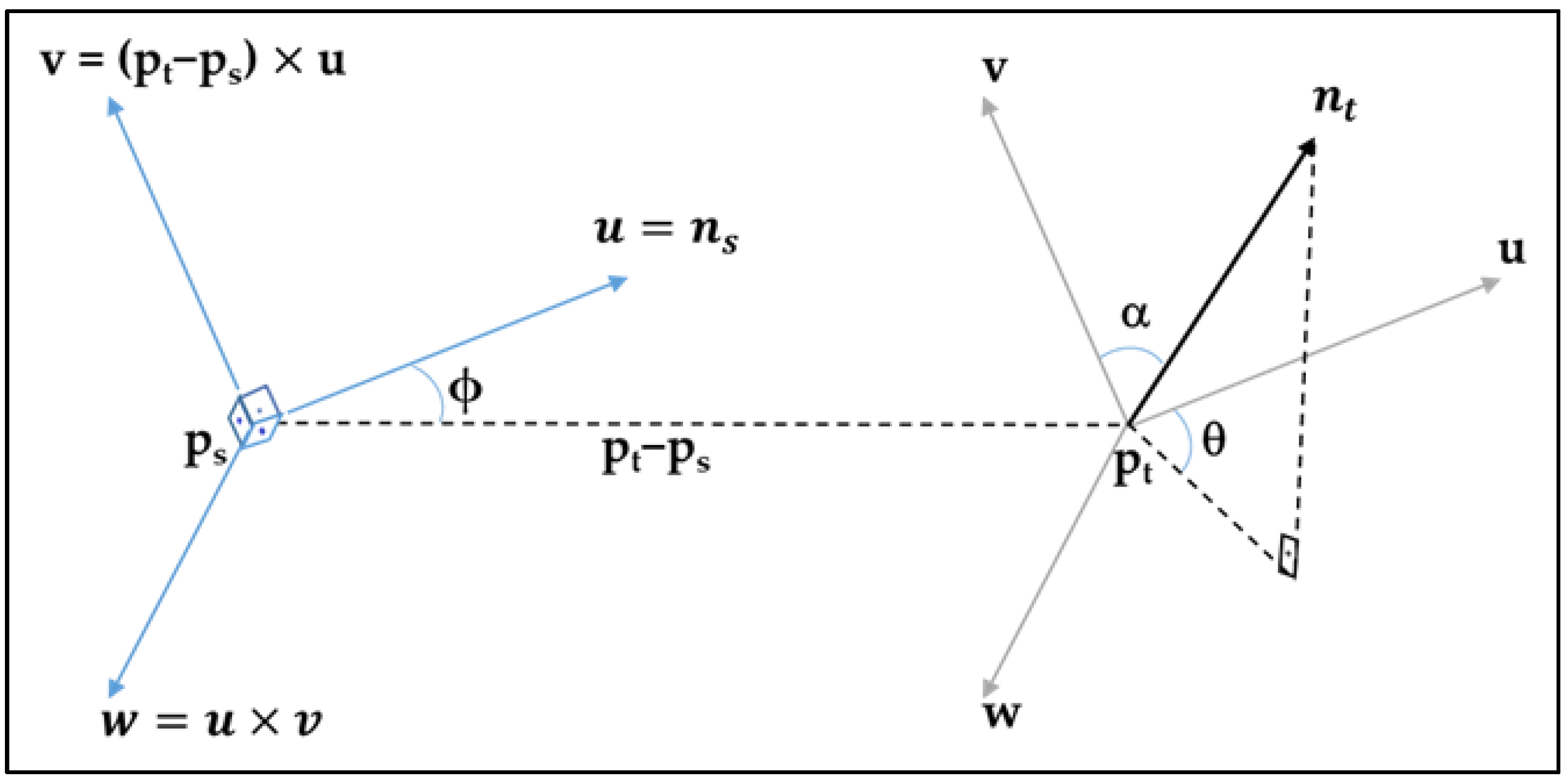
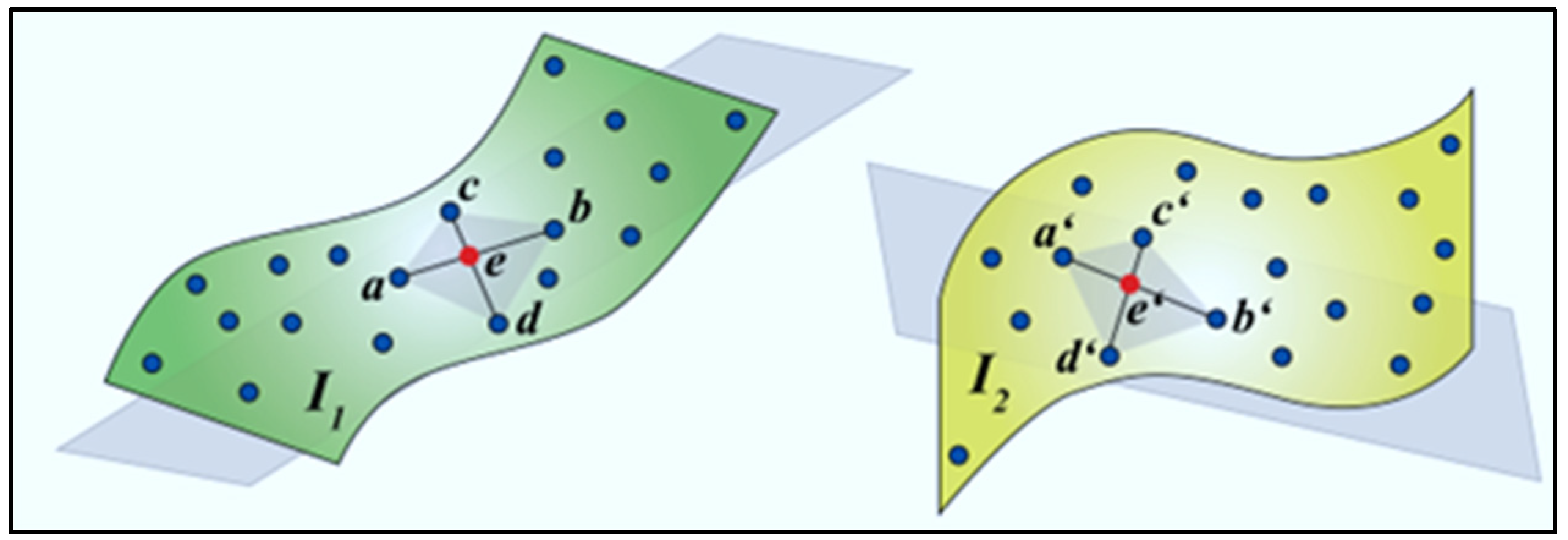
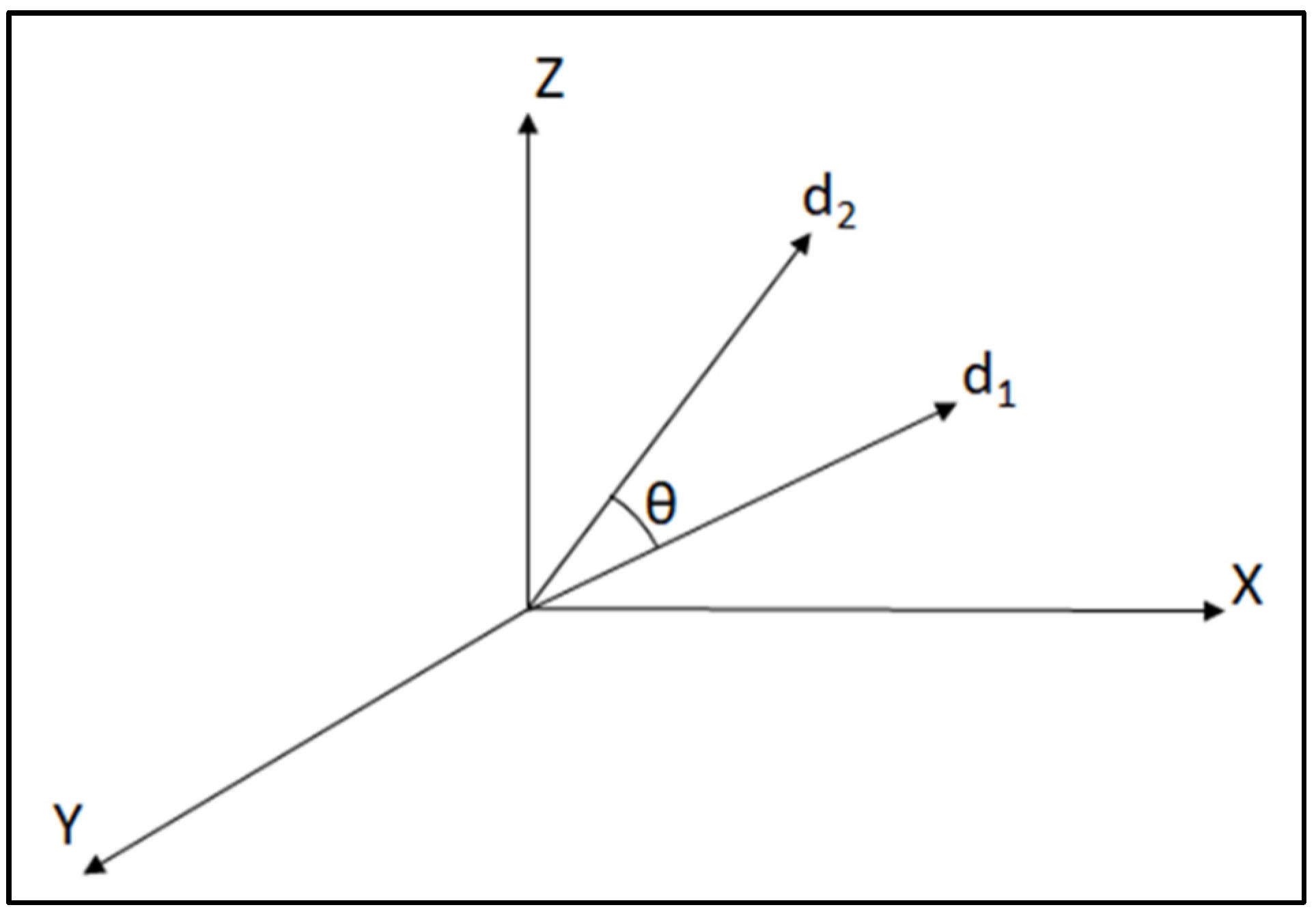
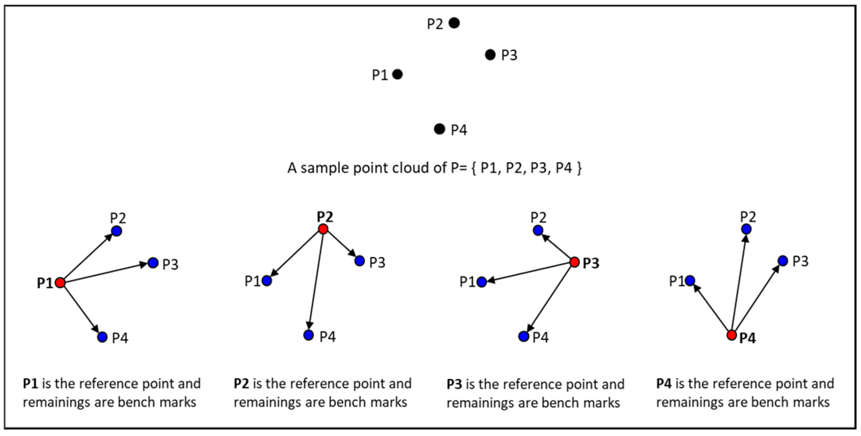
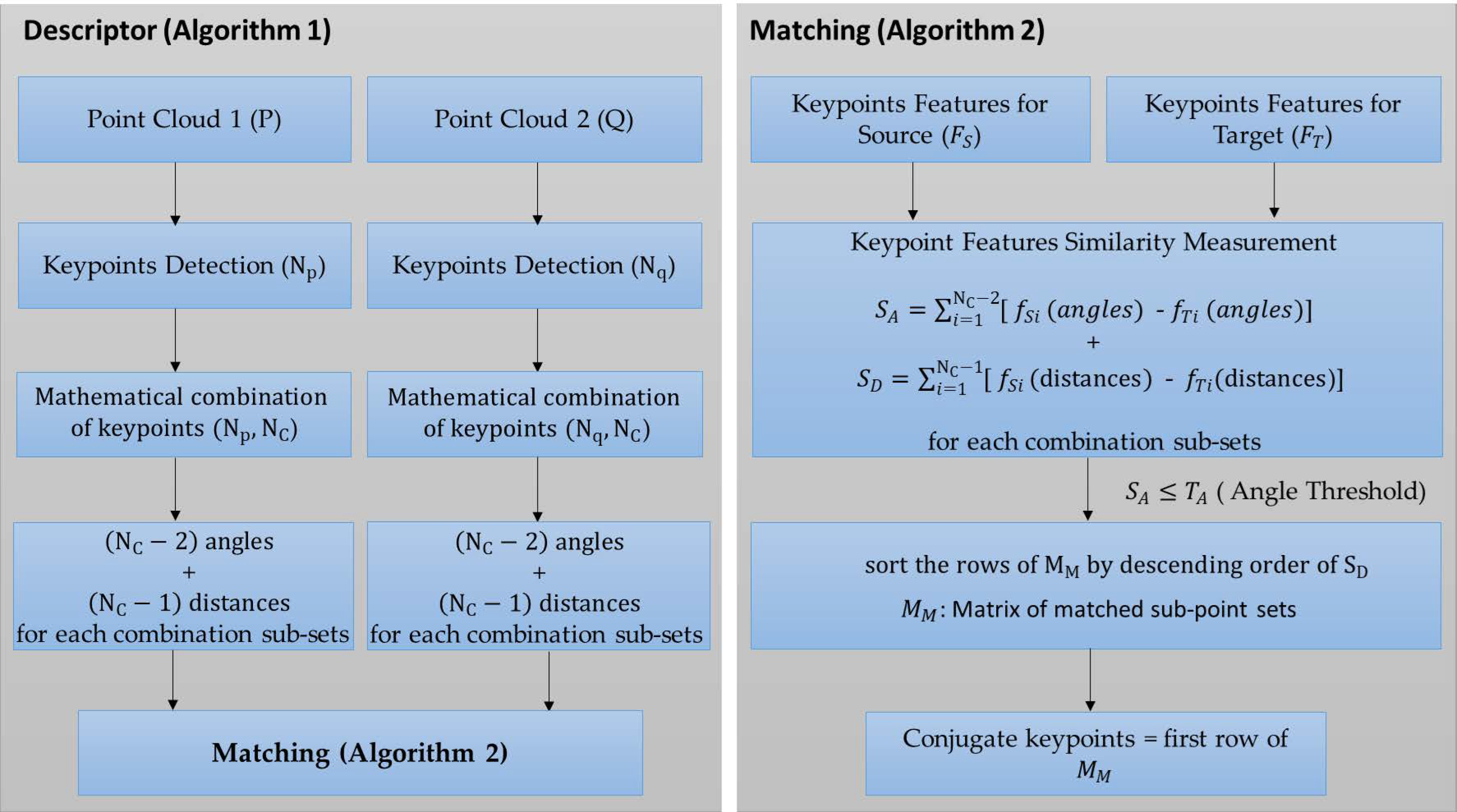
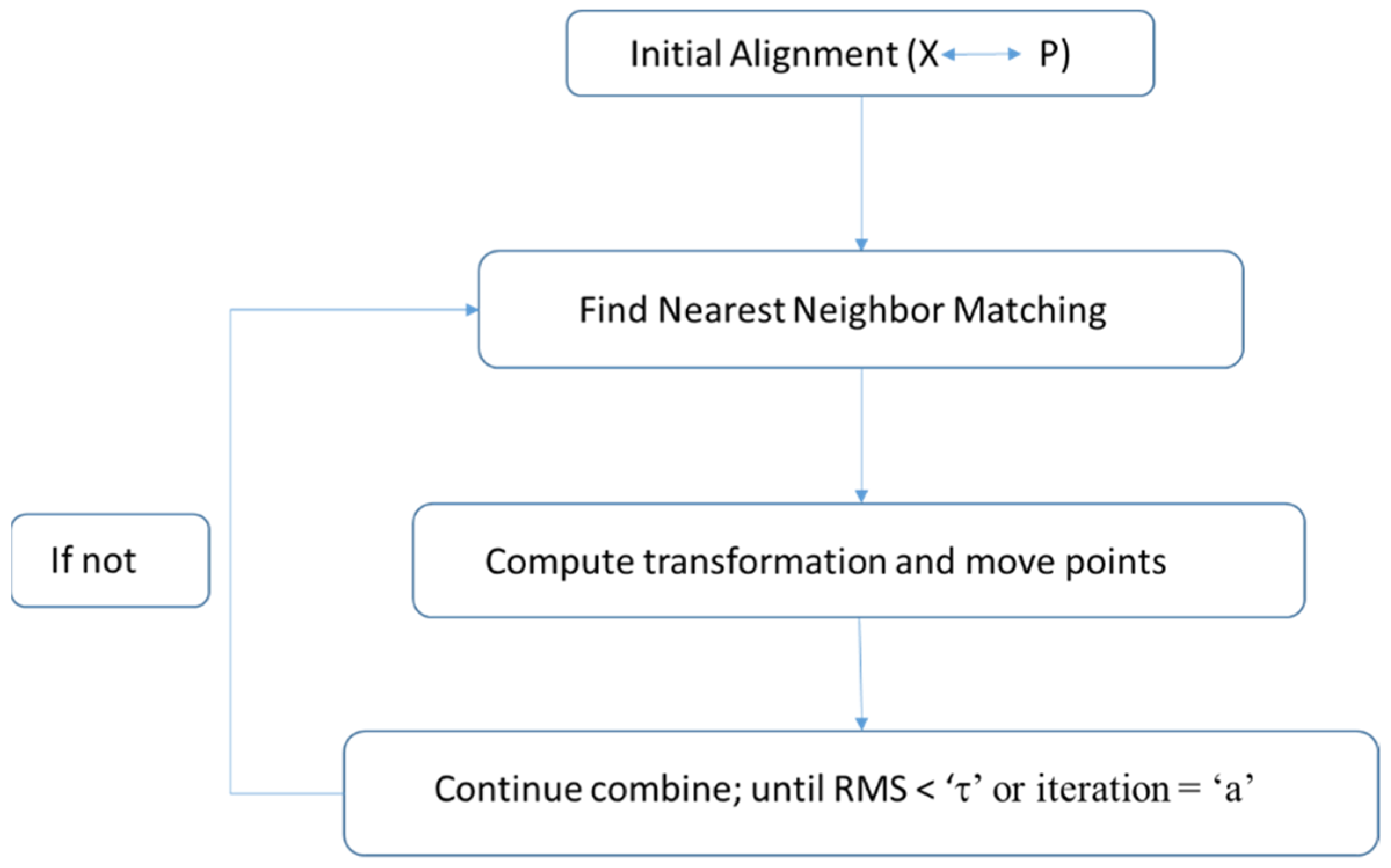
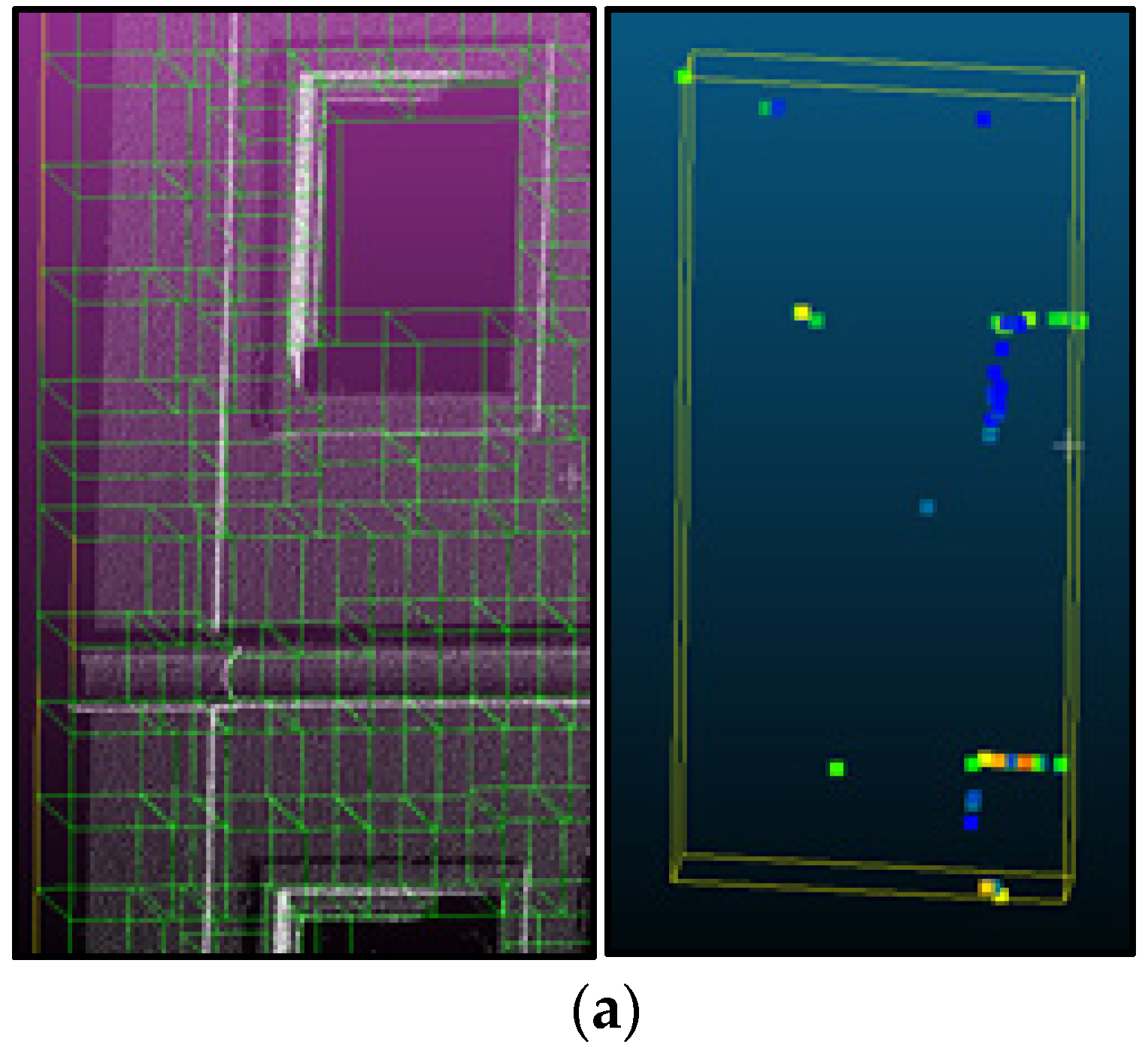
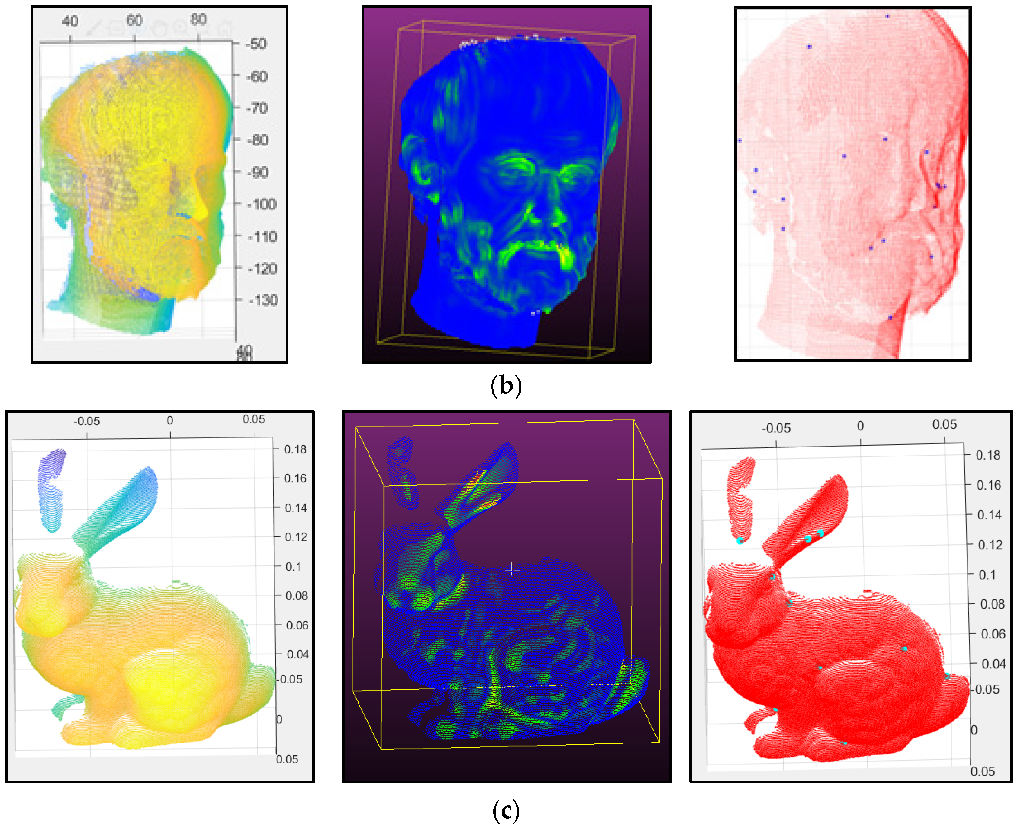
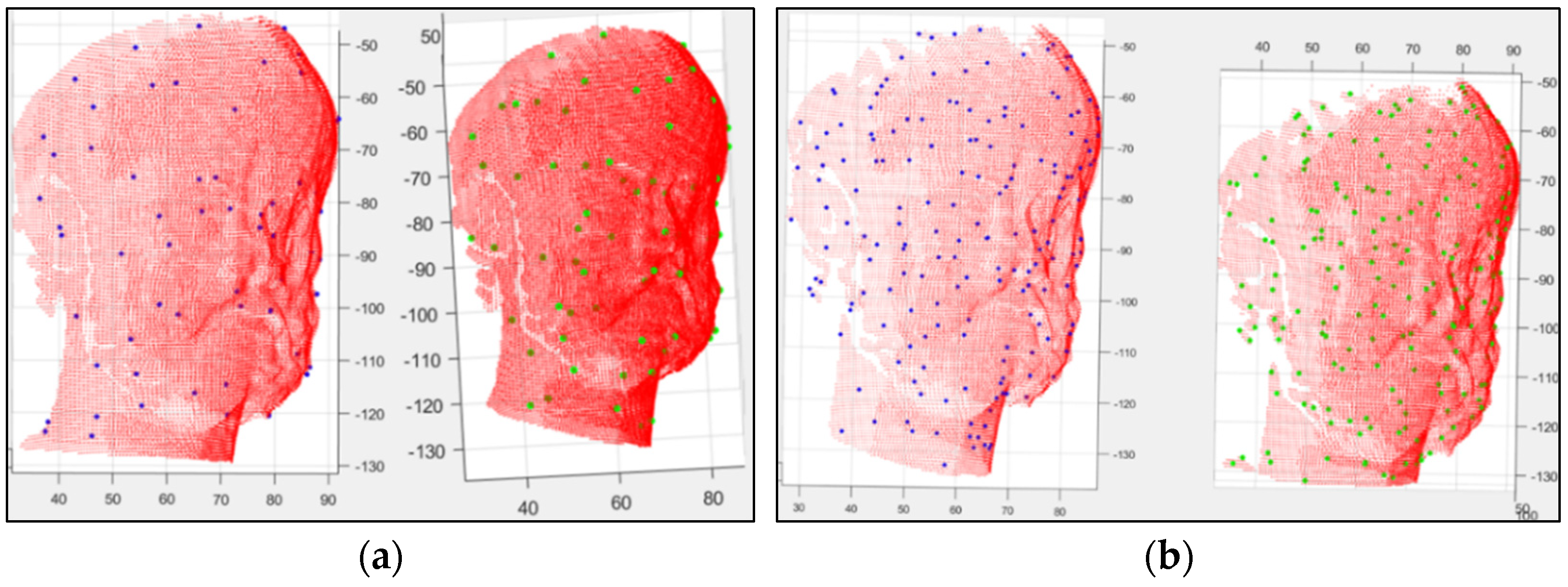
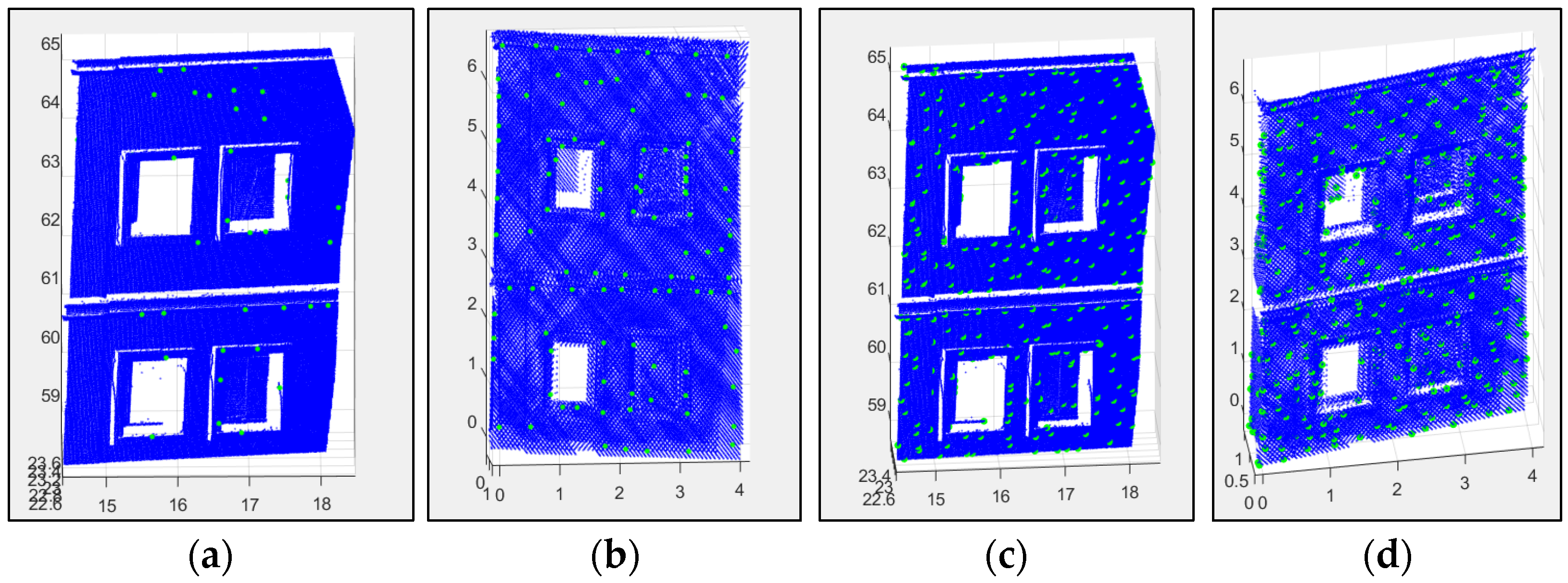
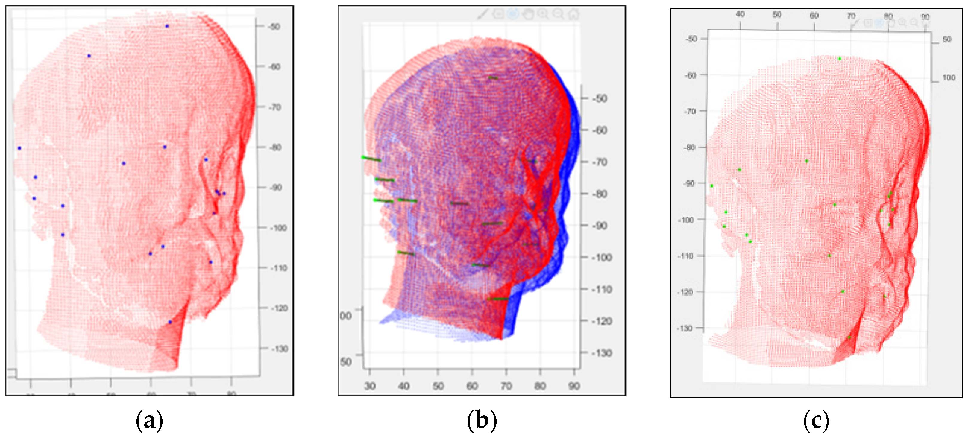
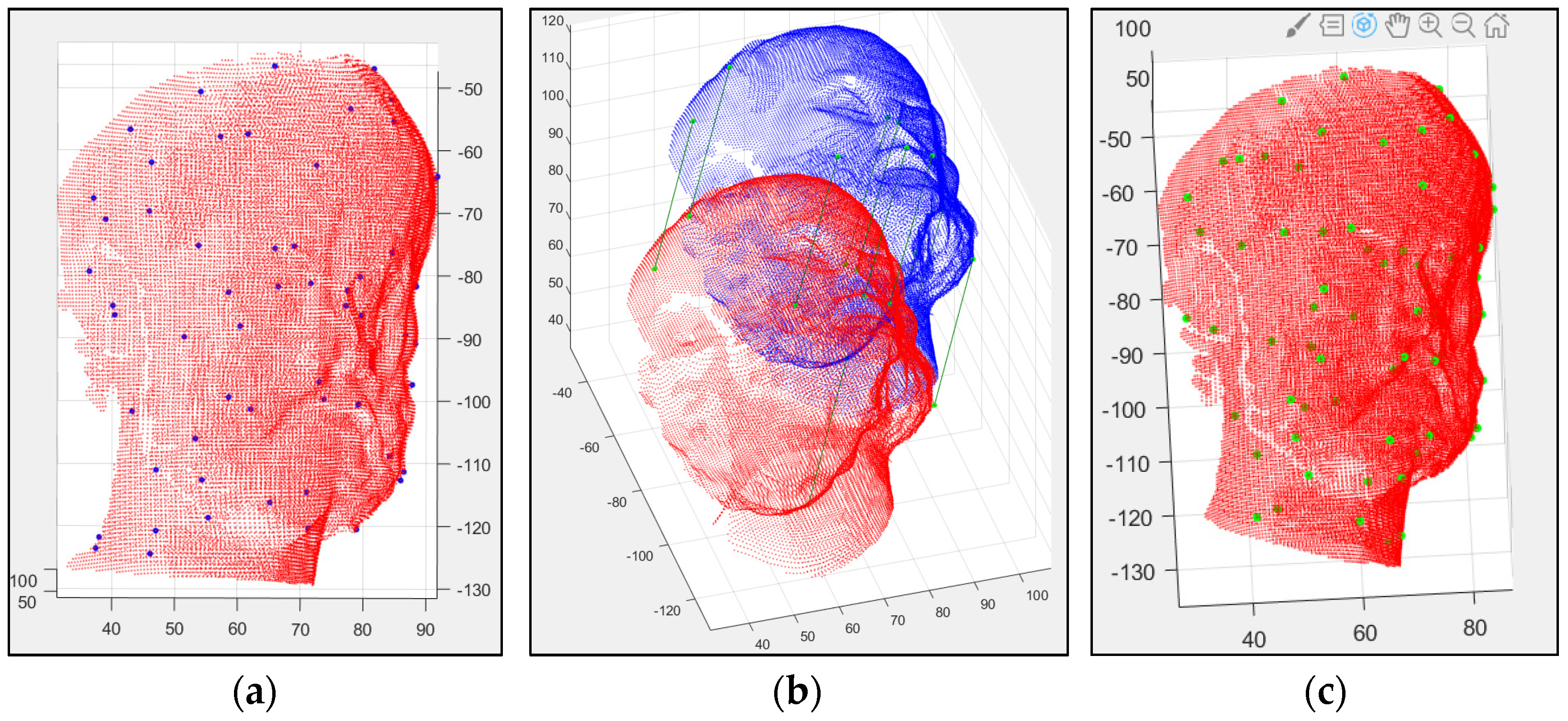
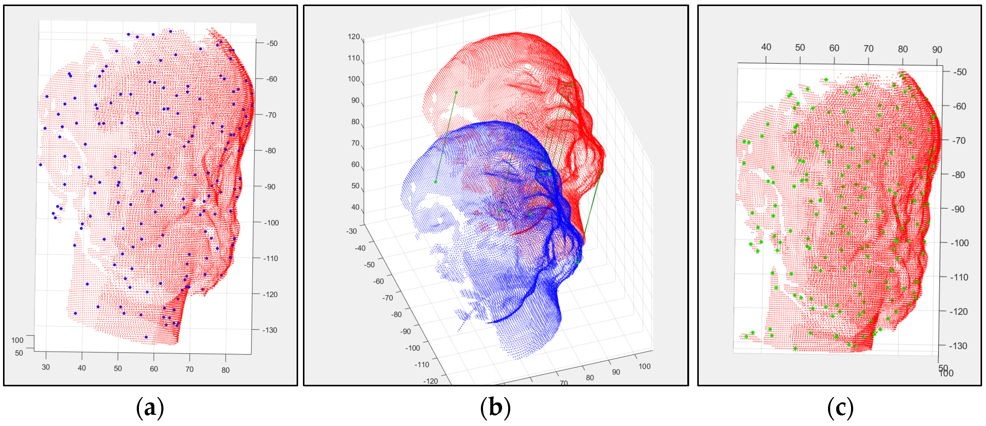
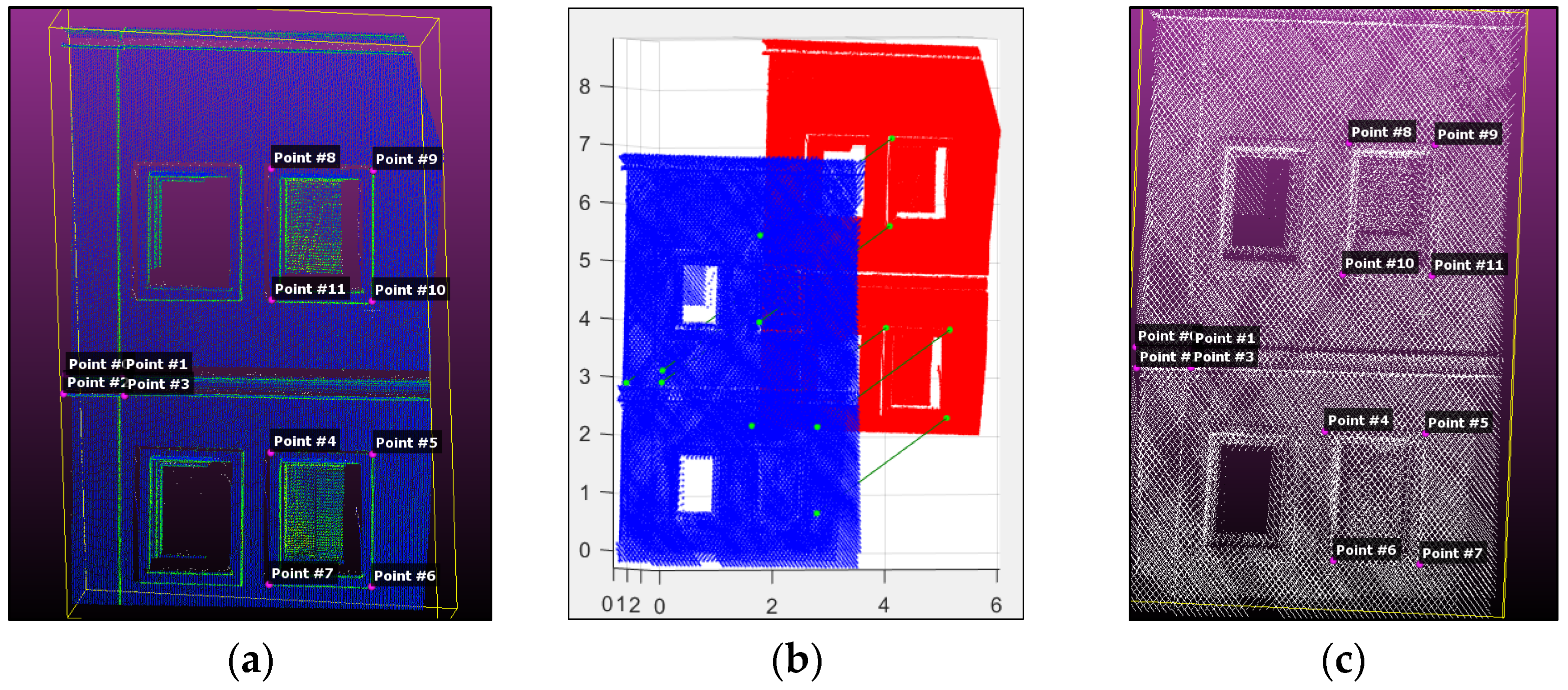
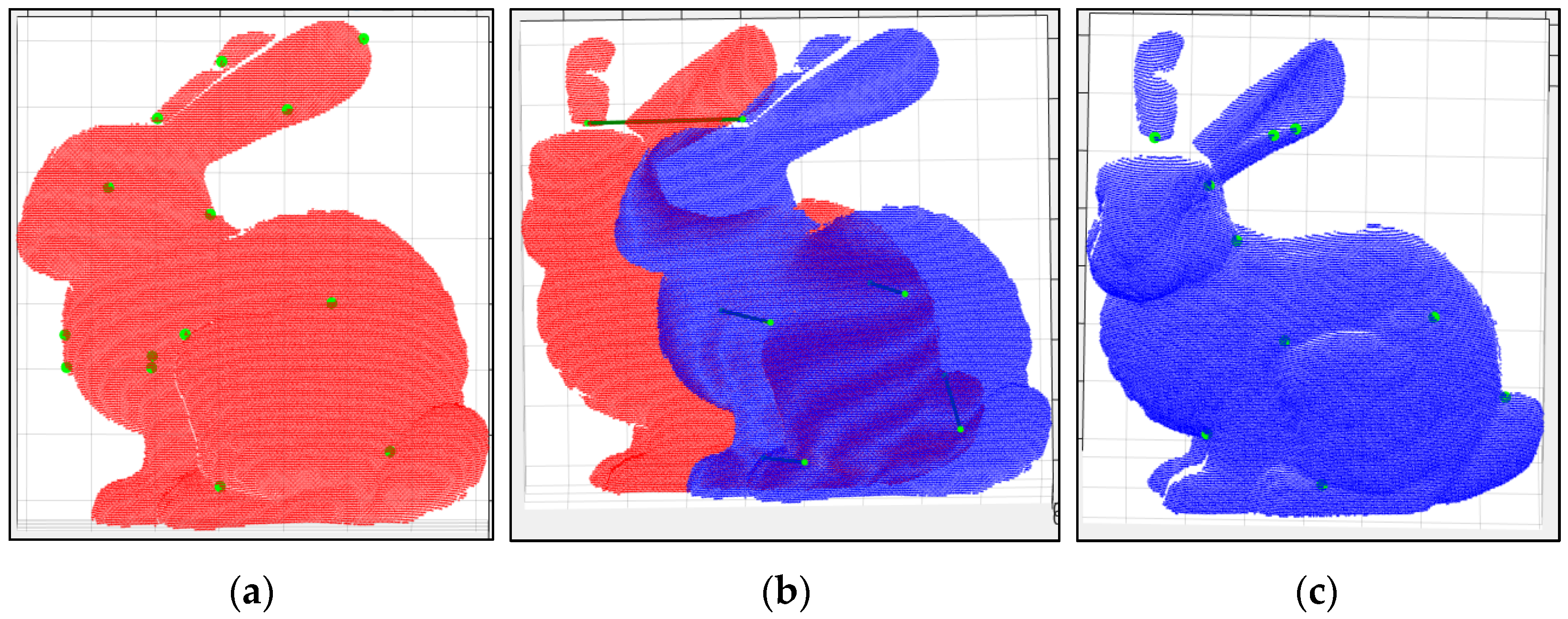
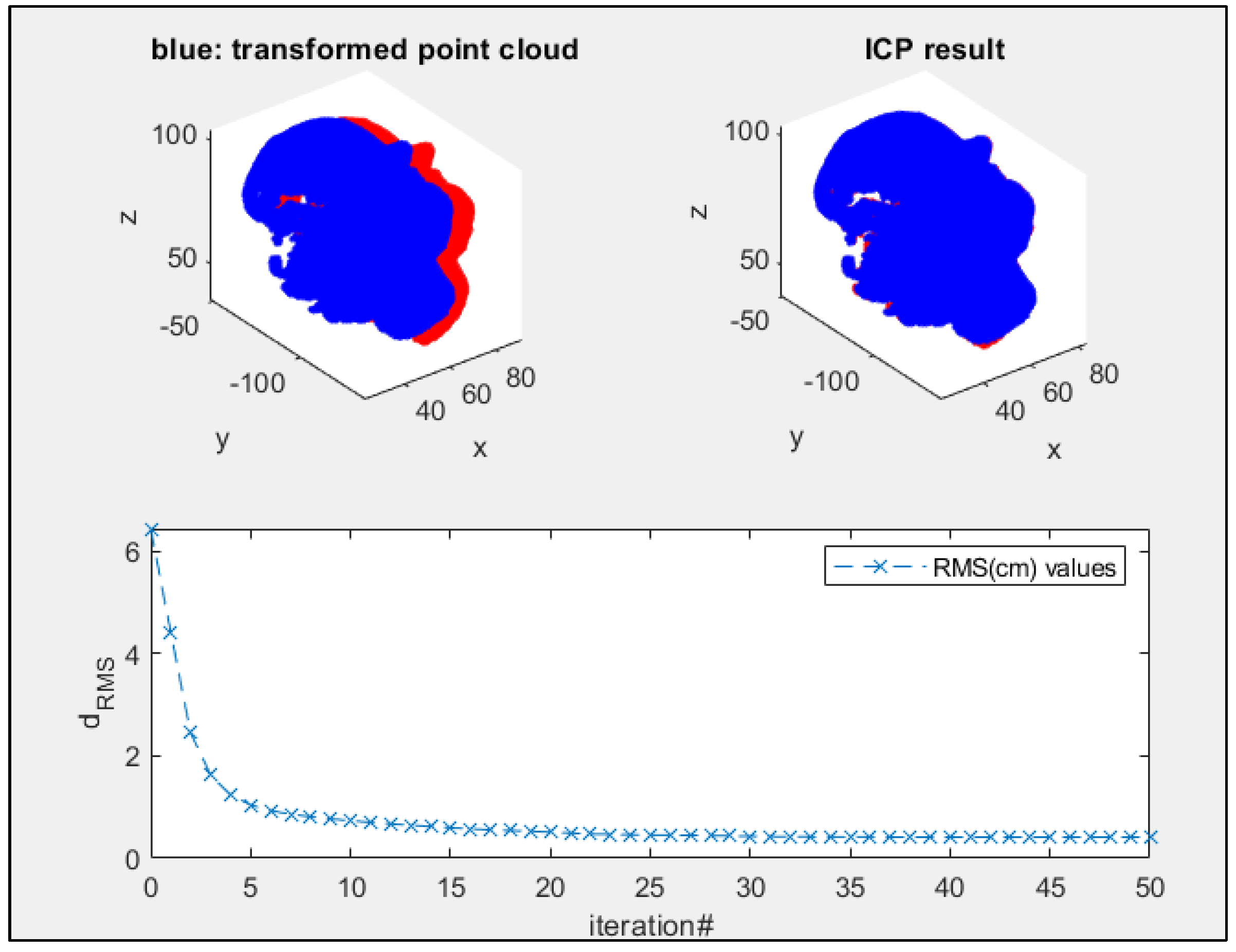
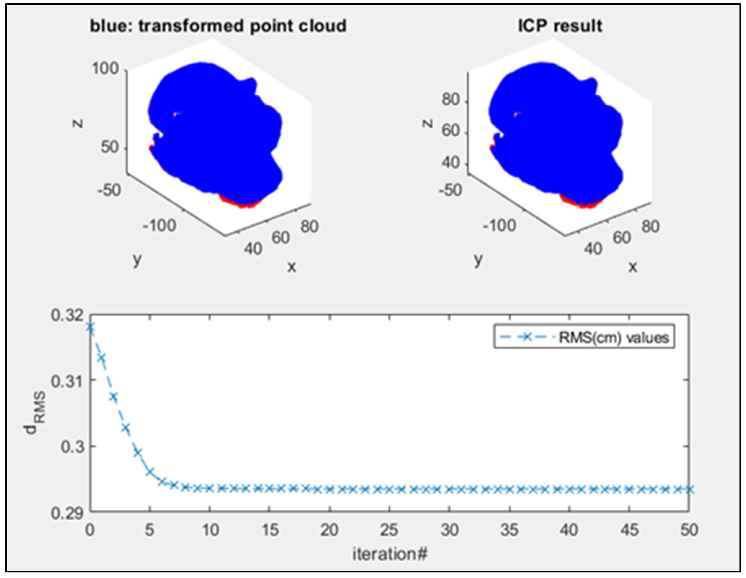
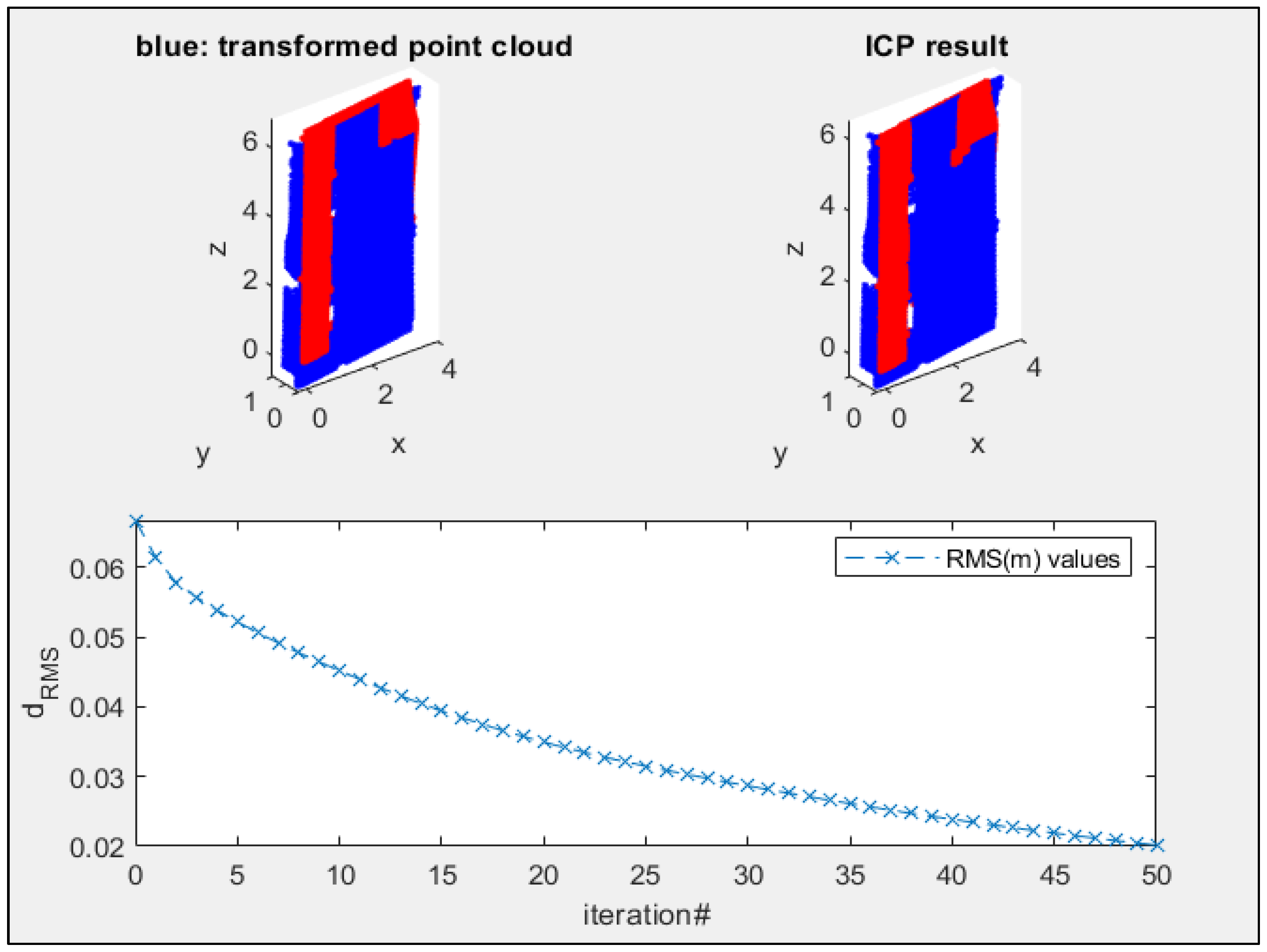
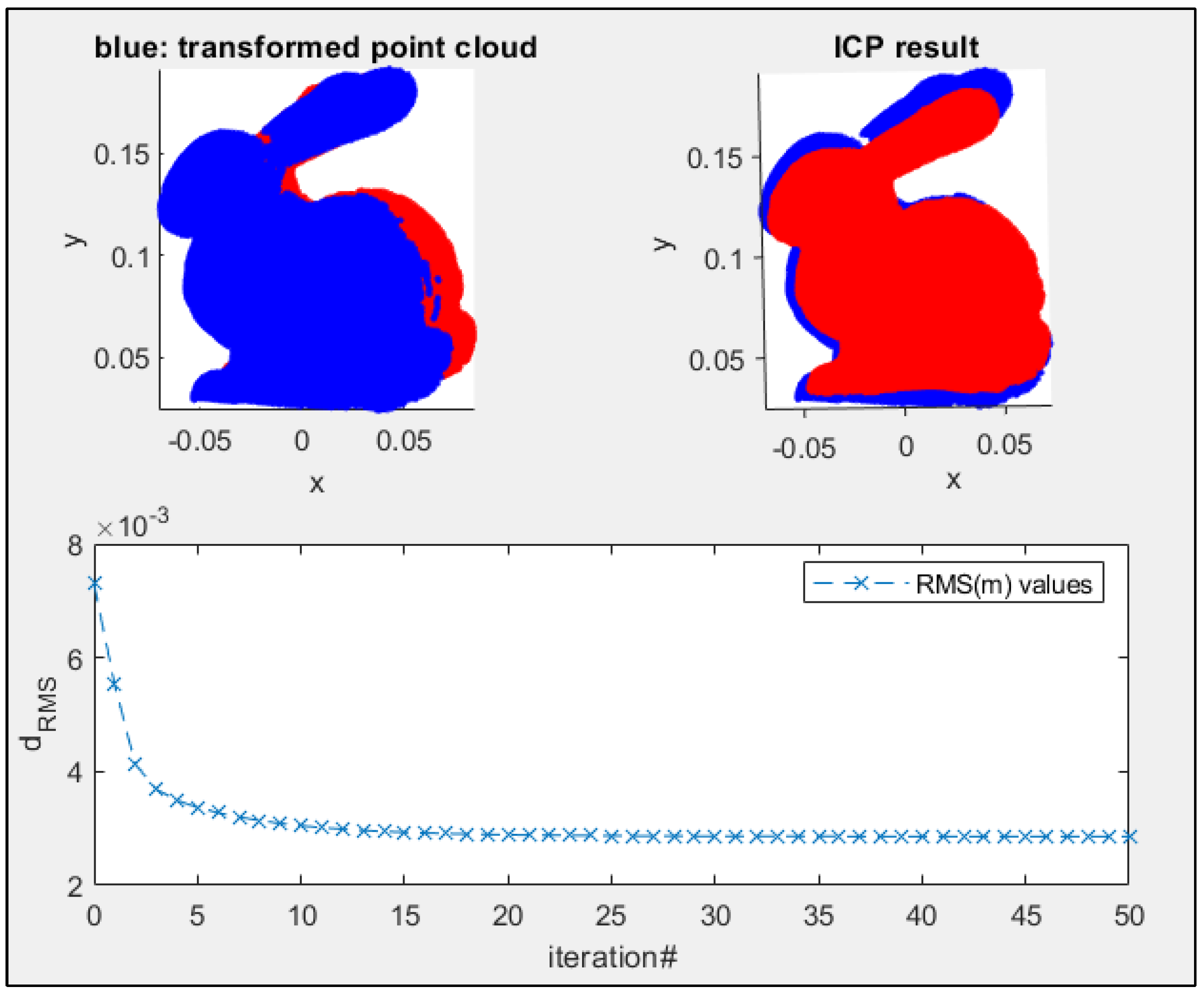
Table 1.
Aristotle sculpture: transformation parameters () with their RMSE (mx) in coarse registration with the ISS+PFH method.
Table 1.
Aristotle sculpture: transformation parameters () with their RMSE (mx) in coarse registration with the ISS+PFH method.
| Parameters | Gauss-Markov | RMSE mx | Gauss-Markov | RMSE mx |
|---|---|---|---|---|
| mo (cm) | 0.2417 | 0.1746 | ||
| (cm) | −5.2107 | 0.5858 | −4.8035 | 0.2615 |
| (cm) | −0.1793 | 0.6005 | 0.1262 | 0.2628 |
| (cm) | 1.3704 | 0.4864 | 1.3367 | 0.2984 |
| s (unitless) | 0.0044 | 0.0033 | 0.0009 | 0.0037 |
| (rad) | 0.0043 | 0.0048 | −0.0057 | 0.0053 |
| (rad) | 0.0020 | 0.0044 | 0.0018 | 0.0021 |
| (rad) | 0.0007 | 0.0040 | −0.0006 | 0.0029 |
Table 2.
Aristotle sculpture: transformation parameters () with their RMSE (mx) in coarse registration with the LSP+PFH method.
Table 2.
Aristotle sculpture: transformation parameters () with their RMSE (mx) in coarse registration with the LSP+PFH method.
| Parameters | Gauss-Markov | RMSE mx | Gauss-Markov | RMSE mx |
|---|---|---|---|---|
| mo (cm) | 0.6500 | 0.3389 | ||
| (cm) | −1.7221 | 2.2380 | −1.8282 | 0.7134 |
| (cm) | −0.8964 | 2.1862 | −3.1901 | 0.6788 |
| (cm) | −2.1867 | 1.8046 | 2.5650 | 0.5924 |
| s (unitless) | 0.0030 | 0.0107 | 0.0373 | 0.0068 |
| (rad) | 0.0247 | 0.0156 | 0.0642 | 0.0094 |
| (rad) | 0.0220 | 0.0143 | 0.0285 | 0.0042 |
| (rad) | 0.0145 | 0.0133 | 0.0319 | 0.0052 |
Table 3.
Aristotle sculpture: transformation parameters () with their RMSE (mx) in coarse registration with the new algorithm.
Table 3.
Aristotle sculpture: transformation parameters () with their RMSE (mx) in coarse registration with the new algorithm.
| Parameters | Gauss-Markov | RMSE mx | Gauss-Markov | RMSE mx |
|---|---|---|---|---|
| mo (cm) | 0.0930 | 0.0550 | ||
| (cm) | 4.4310 | 0.2810 | 4.2760 | 0.1070 |
| (cm) | −0.0490 | 0.3330 | −0.2050 | 0.1070 |
| (cm) | −1.3570 | 0.3060 | −1.2490 | 0.1030 |
| s (unitless) | −0.0020 | 0.0010 | 0.0011 | 0.0010 |
| (rad) | −0.0020 | 0.0020 | 0.0060 | 0.0010 |
| (rad) | −0.0020 | 0.0010 | −0.0040 | 0.0010 |
| (rad) | −0.0040 | 0.0020 | −0.0030 | 0.0010 |
Table 4.
Building facade: transformation parameters () with their RMSE (mx) in coarse registration with the new algorithm.
Table 4.
Building facade: transformation parameters () with their RMSE (mx) in coarse registration with the new algorithm.
| Parameters | Gauss-Markov | RMSE mx | Gauss-Markov | RMSE mx |
|---|---|---|---|---|
| mo (m) | 0.0207 | 0.0143 | ||
| (m) | −0.1355 | 0.0166 | −0.1245 | 0.0090 |
| (m) | 0.0186 | 0.0241 | 0.0152 | 0.0091 |
| (m) | −0.2893 | 0.0162 | −0.3021 | 0.0097 |
| s (unitless) | -0.0016 | 0.0041 | −0.0063 | 0.0032 |
| (rad) | −0.0017 | 0.0057 | −0.0082 | 0.0044 |
| (rad) | −0.0023 | 0.0042 | −0.0013 | 0.0010 |
| (rad) | −0.0002 | 0.0064 | −0.0021 | 0.0012 |
Table 5.
Stanford bunny sculpture: transformation parameters () with their RMSE (mx) in coarse registration with the new algorithm.
Table 5.
Stanford bunny sculpture: transformation parameters () with their RMSE (mx) in coarse registration with the new algorithm.
| Parameters | Gauss-Markov | RMSE mx | Gauss-Markov | RMSE mx |
|---|---|---|---|---|
| mo (m) | 0.0072 | 0.0051 | ||
| (m) | 0.0218 | 0.0077 | 0.0270 | 0.0066 |
| (m) | 0.0092 | 0.0068 | −0.0183 | 0.0058 |
| (m) | 0.0405 | 0.0092 | 0.0426 | 0.0045 |
| s (unitless) | −0.1443 | 0.0550 | 0.0990 | 0.0425 |
| (rad) | −0.0012 | 0.0927 | −0.0072 | 0.0596 |
| (rad) | 0.5441 | 0.0845 | 0.6985 | 0.0687 |
| (rad) | 0.1349 | 0.0609 | 0.0778 | 0.0579 |
Publisher’s Note: MDPI stays neutral with regard to jurisdictional claims in published maps and institutional affiliations. |
© 2021 by the authors. Licensee MDPI, Basel, Switzerland. This article is an open access article distributed under the terms and conditions of the Creative Commons Attribution (CC BY) license (http://creativecommons.org/licenses/by/4.0/).
Share and Cite
MDPI and ACS Style
Kuçak, R.A.; Erol, S.; Erol, B. An Experimental Study of a New Keypoint Matching Algorithm for Automatic Point Cloud Registration. ISPRS Int. J. Geo-Inf. 2021, 10, 204. https://0-doi-org.brum.beds.ac.uk/10.3390/ijgi10040204
AMA Style
Kuçak RA, Erol S, Erol B. An Experimental Study of a New Keypoint Matching Algorithm for Automatic Point Cloud Registration. ISPRS International Journal of Geo-Information. 2021; 10(4):204. https://0-doi-org.brum.beds.ac.uk/10.3390/ijgi10040204
Chicago/Turabian StyleKuçak, Ramazan Alper, Serdar Erol, and Bihter Erol. 2021. "An Experimental Study of a New Keypoint Matching Algorithm for Automatic Point Cloud Registration" ISPRS International Journal of Geo-Information 10, no. 4: 204. https://0-doi-org.brum.beds.ac.uk/10.3390/ijgi10040204
Note that from the first issue of 2016, this journal uses article numbers instead of page numbers. See further details here.