Remote Sensing Data Assimilation in Dynamic Crop Models Using Particle Swarm Optimization


Abstract
:1. Introduction
2. Materials and Methods
2.1. Datasets
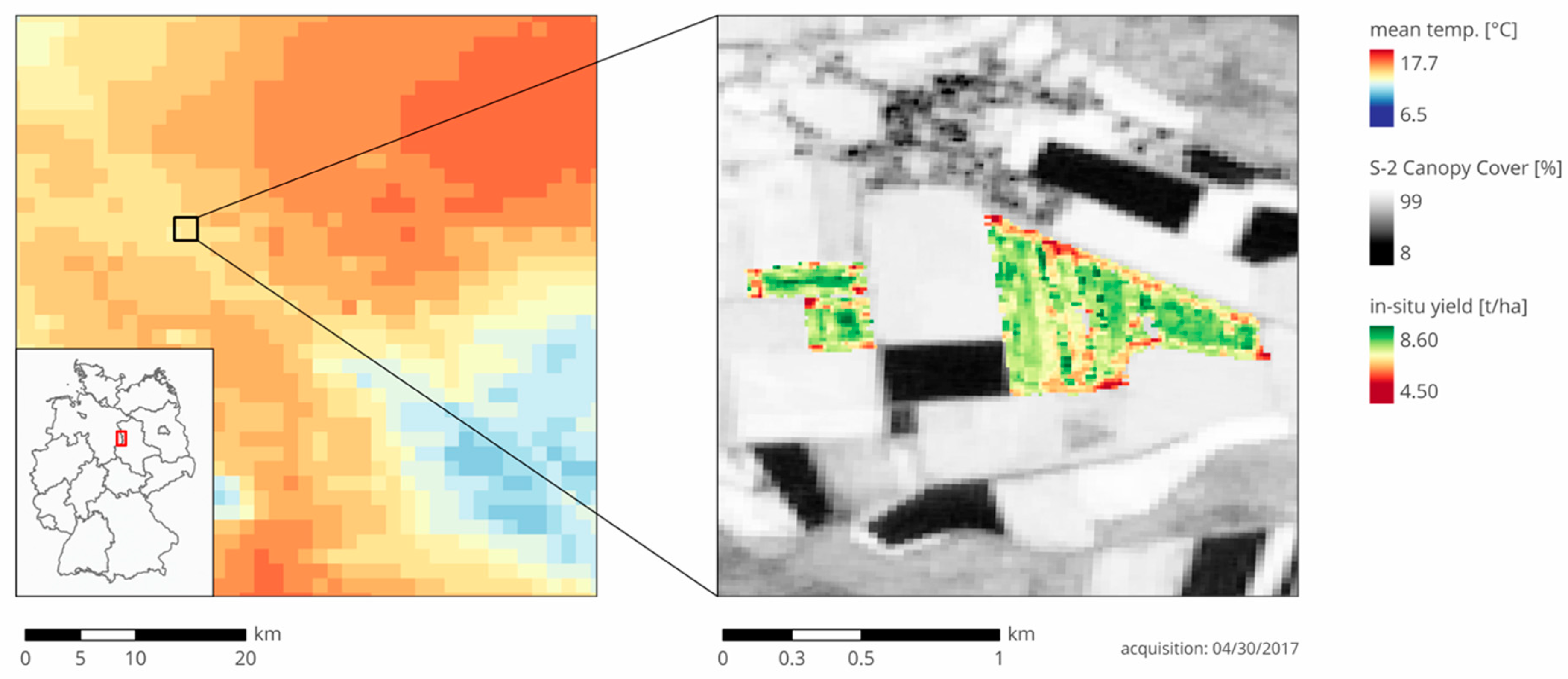
2.1.1. Study Area
2.1.2. Weather Data
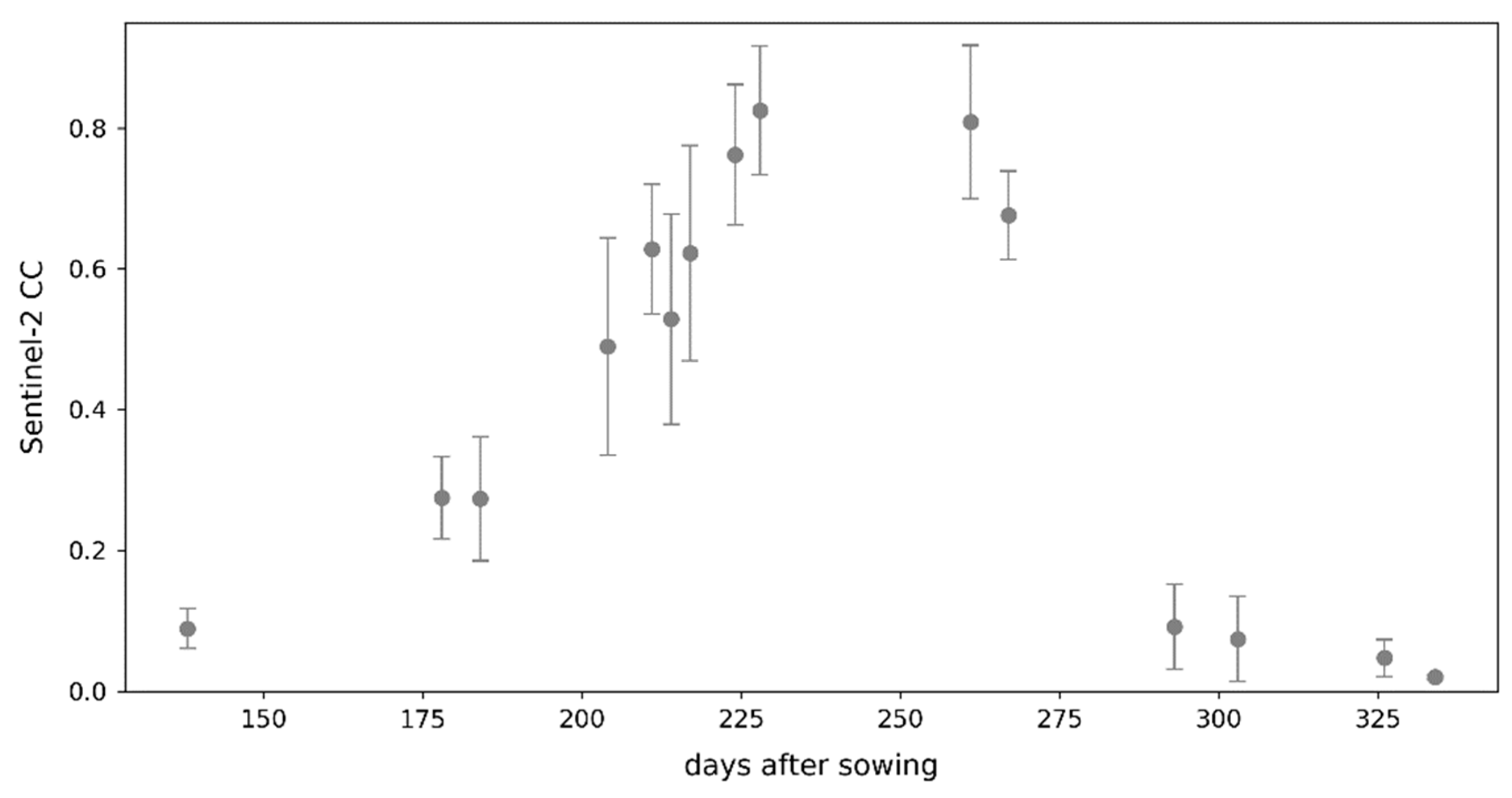
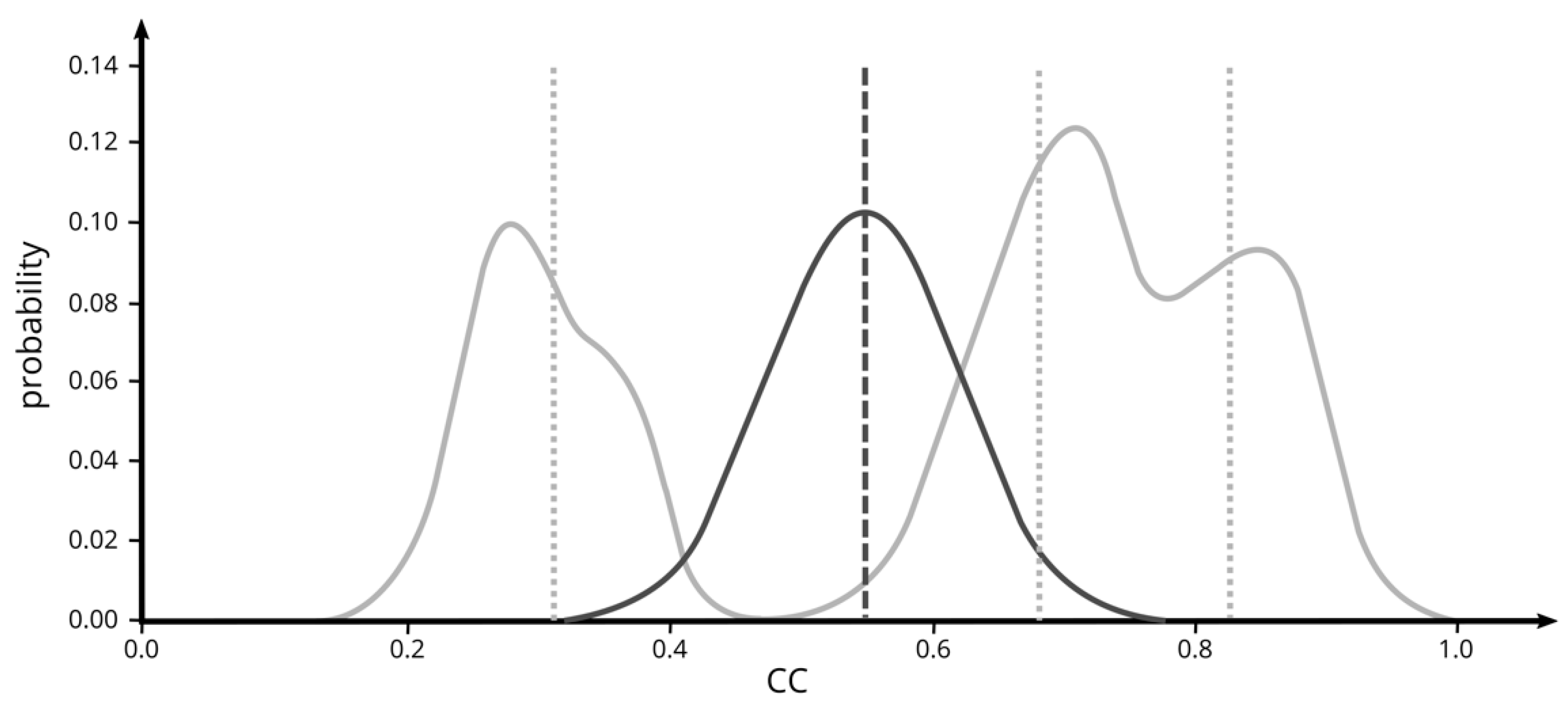
2.1.3. Canopy Cover Data
2.1.4. Yield Data
2.2. Methodological Background
2.2.1. AquaCrop-OS Description
2.2.2. AquaCrop-OS Calibration
2.2.3. Particle Swarm Optimization
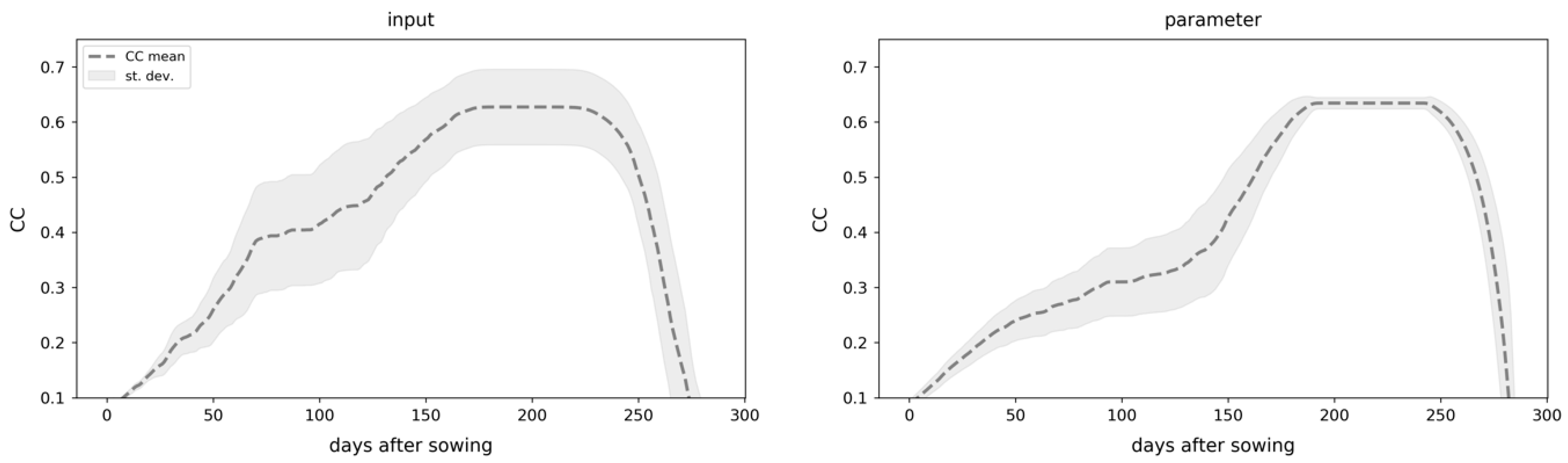
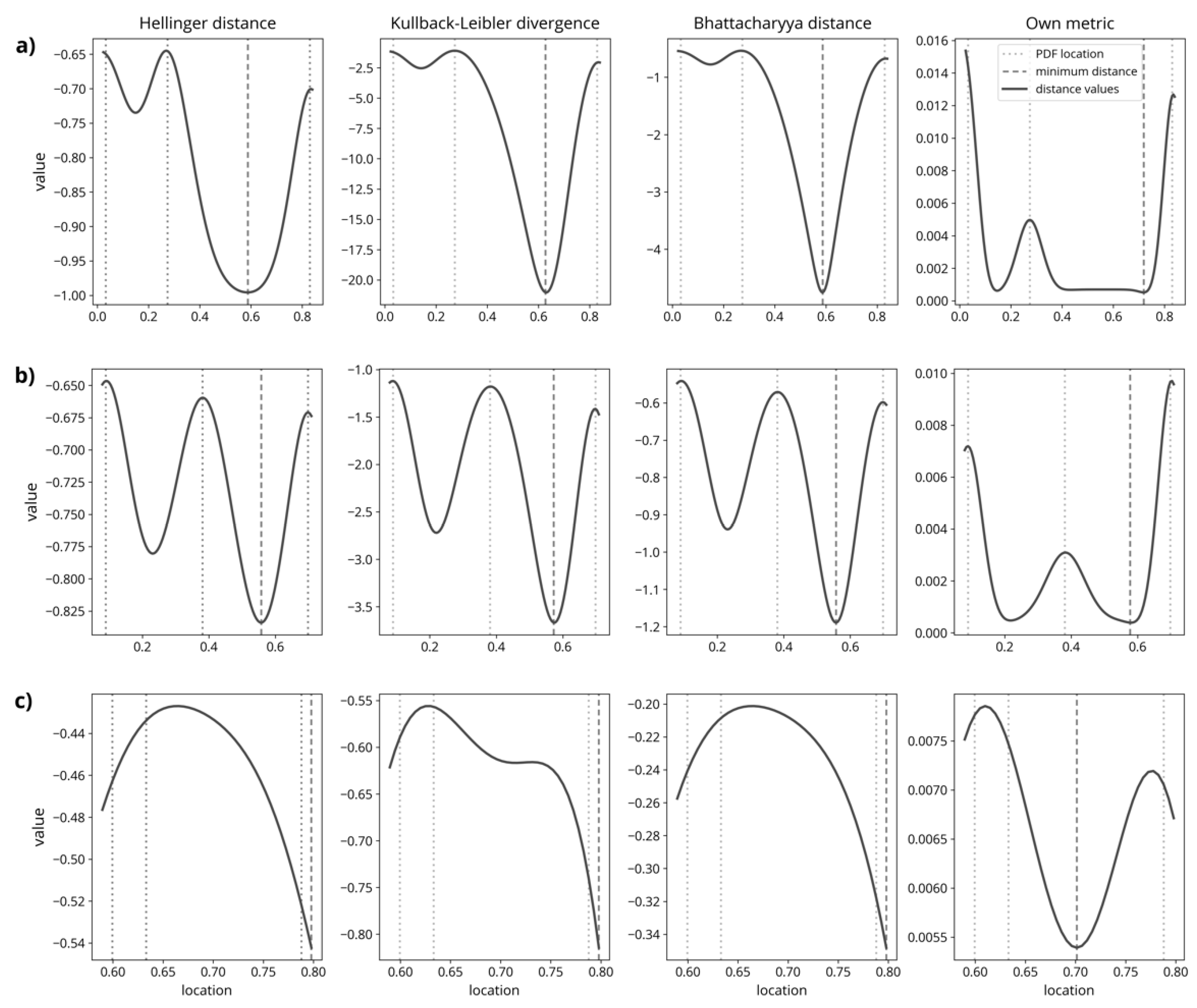
2.2.4. Uncertainty Quantification
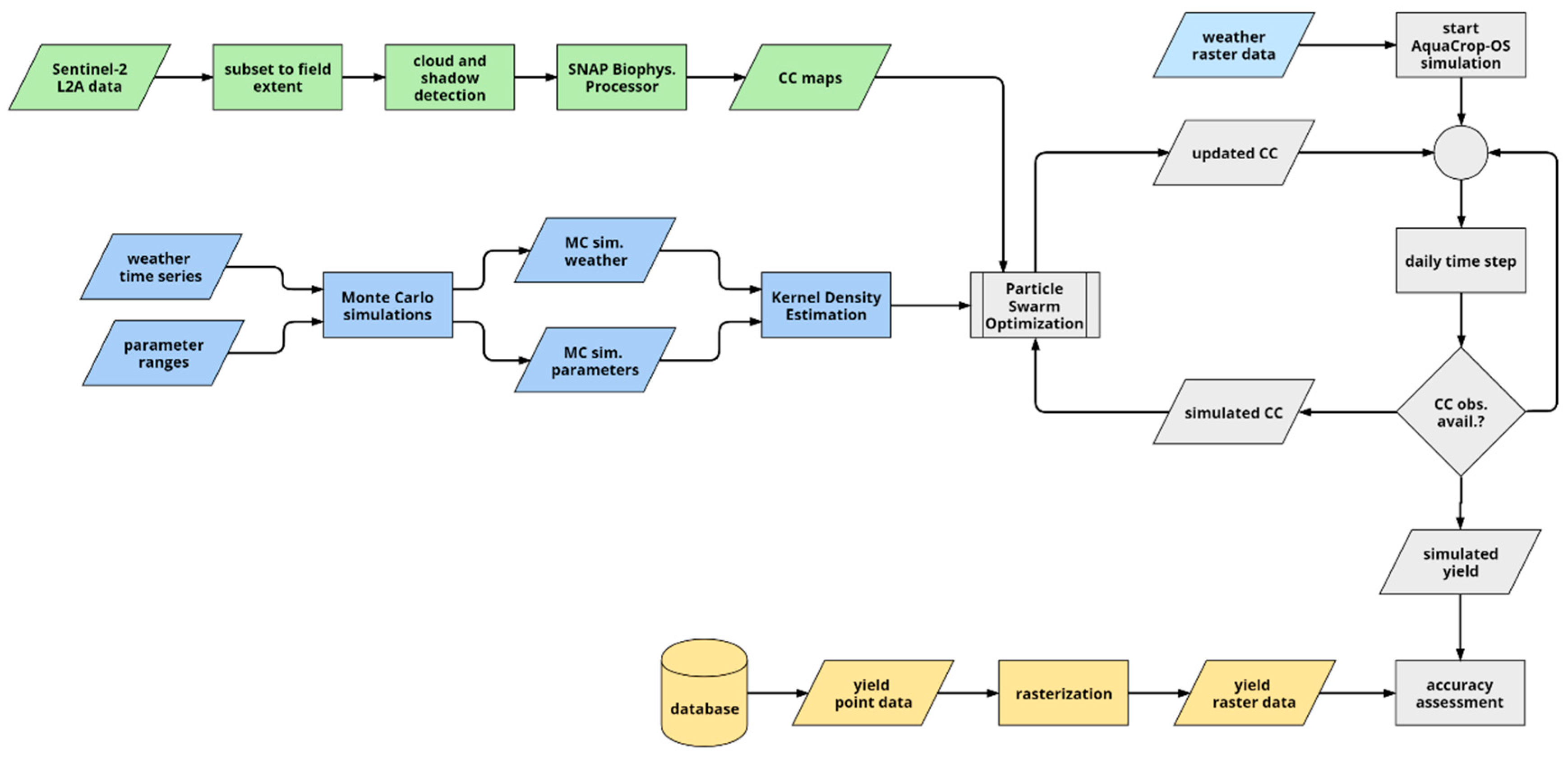
2.3. Updating Methodology
2.3.1. Simple Updating
2.3.2. Extended Kalman Filter Updating
2.3.3. New Updating Scheme
2.3.4. Performance Analysis
3. Results
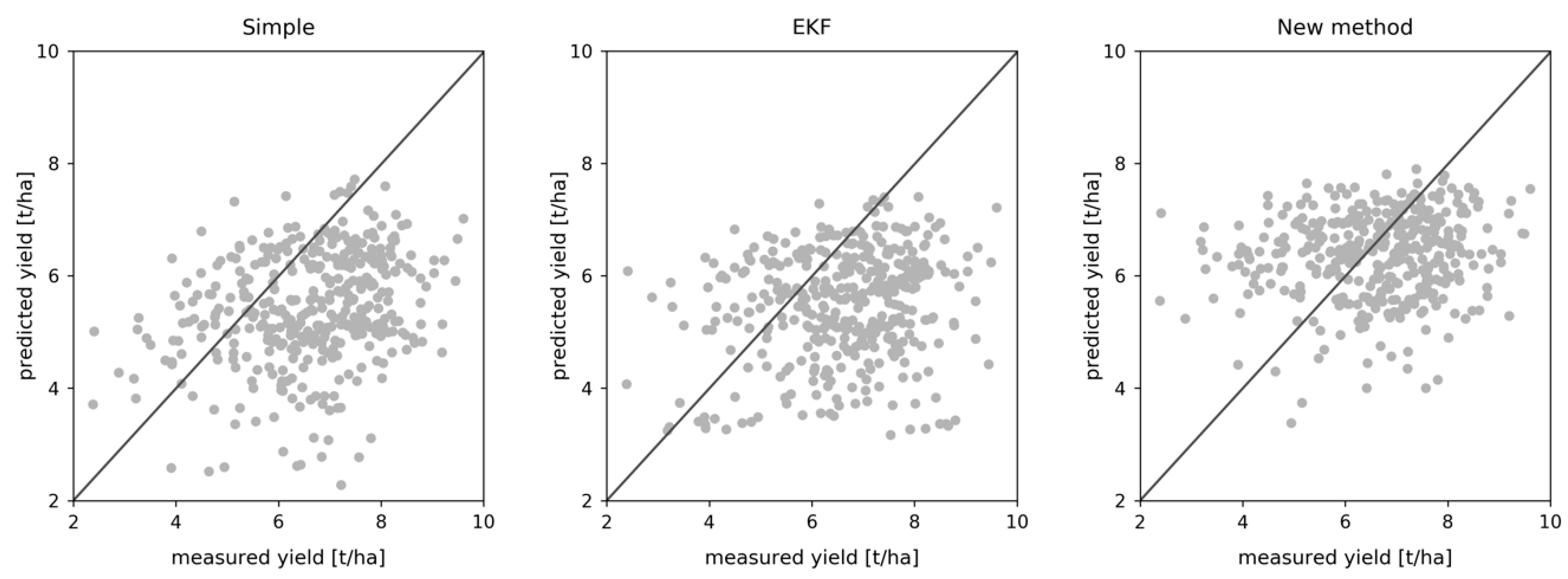
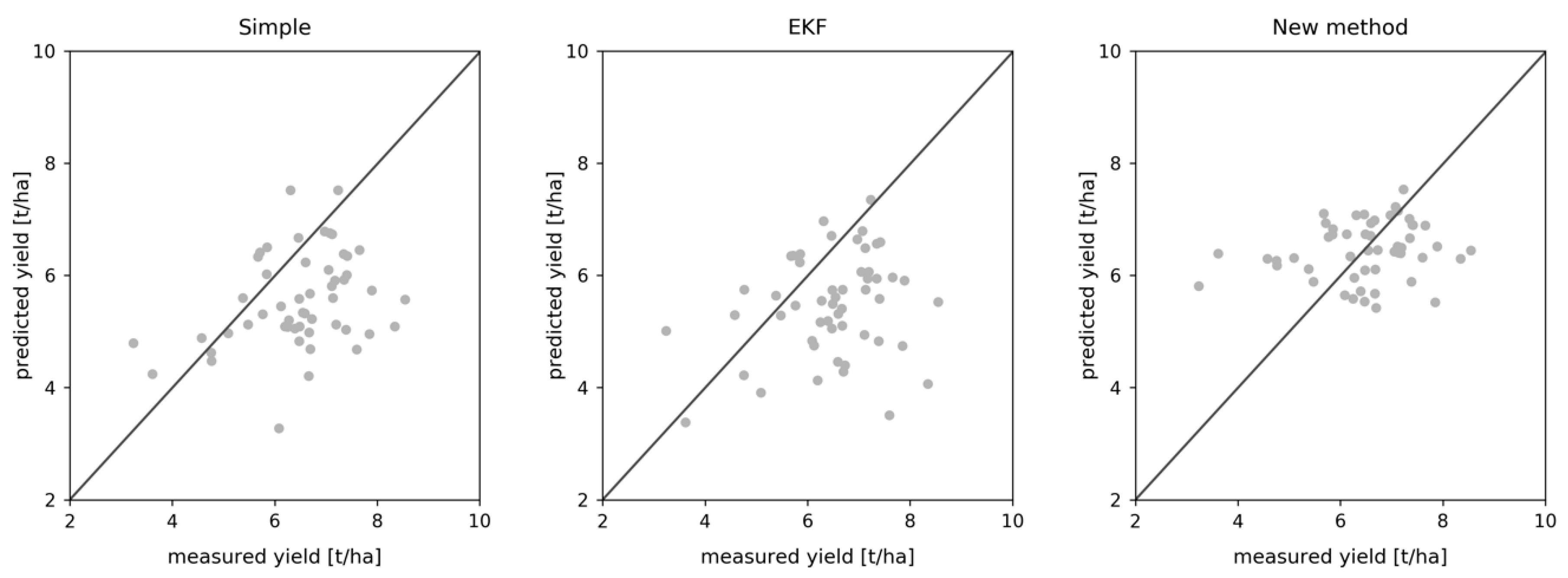
3.1. Field-Level Yield Estimation
3.2. Pixel-Level Yield Estimation
3.3. Pixel-To-Field Aggregated Yield Estimation
3.4. R2 Performance
4. Discussion
5. Conclusions
Author Contributions
Funding
Acknowledgments
Conflicts of Interest
References
- Asseng, S.; Ewert, F.; Martre, P.; Rötter, R.P.; Lobell, D.B.; Cammarano, D.; Kimball, B.A.; Ottman, M.J.; Wall, G.W.; White, J.W.; et al. Rising temperatures reduce global wheat production. Nat. Clim. Chang. 2015, 5, 143–147. [Google Scholar] [CrossRef]
- Food and Agriculture Organization of the United Nations. Climate Change and Food Systems—Global Assessments and Implications for Food Security and Trade; Elbehri, A., Ed.; FAO: Rome, Italy, 2015. [Google Scholar]
- Alexandratos, N.; Bruinsma, J. World Agriculture towards 2030/2050: The 2012 Revision; Food and Agriculture Organization of the United Nations: Rome, Italy, 2012; ISBN 9789251086995. [Google Scholar]
- United Nations, Department of Economic and Social Affairs. Population Division World Population Prospects—The 2017 Revision, Key Findings and Advance Tables; United Nations, Department of Economic and Social Affairs, Population Division: New York, NY, USA, 2015. [Google Scholar]
- Basso, B.; Cammarano, D.; Carfagna, E. Review of Crop Yield Forecasting Methods and Early Warning Systems. In Proceedings of the First Meeting of the Scientific Advisory Committee of the Global Strategy to Improve Agricultural and Rural Statistics, Rome, Italy, 18–19 July 2013. [Google Scholar]
- Jones, J.W.; Antle, J.M.; Basso, B.; Boote, K.J.; Conant, R.T.; Foster, I.; Godfray, H.C.J.; Herrero, M.; Howitt, R.E.; Janssen, S.; et al. Toward a new generation of agricultural system data, models, and knowledge products: State of agricultural systems science. Agric. Syst. 2017, 155, 269–288. [Google Scholar] [CrossRef] [PubMed]
- Delécolle, R.; Maas, S.J.; Guérif, M.; Baret, F. Remote sensing and crop production models: Present trends. ISPRS J. Photogramm. Remote Sens. 1992, 47, 145–161. [Google Scholar] [CrossRef]
- Rembold, F.; Atzberger, C.; Savin, I.; Rojas, O. Using low resolution satellite imagery for yield prediction and yield anomaly detection. Remote Sens. 2013, 5, 1704–1733. [Google Scholar] [CrossRef] [Green Version]
- Maas, S.J. Use of remotely-sensed information in agricultural crop growth models. Ecol. Modell. 1988, 41, 247–268. [Google Scholar] [CrossRef]
- Dorigo, W.A.; Zurita-Milla, R.; de Wit, A.J.W.; Brazile, J.; Singh, R.; Schaepman, M.E. A review on reflective remote sensing and data assimilation techniques for enhanced agroecosystem modeling. Int. J. Appl. Earth Obs. Geoinf. 2007, 9, 165–193. [Google Scholar] [CrossRef]
- Kalman, R.E. A New Approach to Linear Filtering and Prediction Problems. Trans. ASME—J. Basic Eng. 1960, 82, 35–45. [Google Scholar] [CrossRef] [Green Version]
- Evensen, G. The Ensemble Kalman Filter: Theoretical formulation and practical implementation. Ocean Dyn. 2003, 53, 343–367. [Google Scholar] [CrossRef]
- Del Moral, P. Nonlinear filtering: Interacting particle resolution. C. R. l’Académie des Sci.—Ser. I Math. 1997, 325, 653–658. [Google Scholar] [CrossRef]
- Kalman, R.E.; Bucy, R.S. New Results in Linear Filtering and Prediction Theory. J. Basic Eng. 1961, 83, 95–108. [Google Scholar] [CrossRef]
- Kennedy, M.C.; O’Hagan, A. Bayesian calibration of computer models. J. R. Stat. Soc. Ser. B Stat. Methodol. 2001, 63, 425–464. [Google Scholar] [CrossRef]
- Asseng, S.; Ewert, F.; Rosenzweig, C.; Jones, J.W.; Hatfield, J.L.; Ruane, A.C.; Boote, K.J.; Thorburn, P.J.; Rötter, R.P.; Cammarano, D.; et al. Uncertainty in simulating wheat yields under climate change. Nat. Clim. Chang. 2013, 3, 827–832. [Google Scholar] [CrossRef] [Green Version]
- Warszawski, L.; Frieler, K.; Huber, V.; Piontek, F.; Serdeczny, O.; Schewe, J. The Inter-Sectoral Impact Model Intercomparison Project (ISI-MIP): Project framework. Proc. Natl. Acad. Sci. USA 2014, 111, 3228–3232. [Google Scholar] [CrossRef] [PubMed] [Green Version]
- Hoffmann, H.; Zhao, G.; van Bussel LG, J.; Enders, A.; Specka, X.; Sosa, C.; Yeluripati, J.; Tao, F.; Constantin, J.; Raynal, H.; et al. Variability of effects of spatial climate data aggregation on regional yield simulation by crop models. Clim. Res. 2015, 65, 53–69. [Google Scholar] [CrossRef] [Green Version]
- van Bussel LG, J.; Ewert, F.; Zhao, G.; Hoffmann, H.; Enders, A.; Wallach, D.; Asseng, S.; Baigorria, G.A.; Basso, B.; Biernath, C.; et al. Spatial sampling of weather data for regional crop yield simulations. Agric. For. Meteorol. 2016, 220, 101–115. [Google Scholar] [CrossRef]
- Reichle, R.H. Data assimilation methods in the Earth sciences. Adv. Water Resour. 2008, 31, 1411–1418. [Google Scholar] [CrossRef]
- Liu, X.P.; Li, X.; Peng, X.J.; Li, H.B.; He, J.Q. Swarm intelligence for classification of remote sensing data. Sci. China Ser. D Earth Sci. 2008, 51, 79–87. [Google Scholar] [CrossRef]
- Shen, L.; Huang, X.; Fan, C. Double-group particle swarm optimization and its application in remote sensing image segmentation. Sensors 2018, 18, 1393. [Google Scholar] [CrossRef]
- Bansal, S.; Gupta, D.; Panchal, V.K.; Kumar, S. Swarm intelligence inspired classifiers in comparison with fuzzy and rough classifiers: A remote sensing approach. Commun. Comput. Inf. Sci. 2009, 40, 284–294. [Google Scholar] [CrossRef]
- Guo, C.; Zhang, L.; Zhou, X.; Zhu, Y.; Cao, W.; Qiu, X.; Cheng, T.; Tian, Y. Integrating remote sensing information with crop model to monitor wheat growth and yield based on simulation zone partitioning. Precis. Agric. 2017, 19, 1–24. [Google Scholar] [CrossRef]
- Omkar, S.N.; Senthilnath, J.; Mudigere, D.; Manoj Kumar, M. Crop Classification using Biologically-inspired Techniques with High Resolution Satellite Image. J. Indian Soc. Remote Sens. 2008, 36, 175–182. [Google Scholar] [CrossRef]
- Jin, M.; Liu, X.; Wu, L.; Liu, M. An improved assimilation method with stress factors incorporated in the WOFOST model for the efficient assessment of heavy metal stress levels in rice. Int. J. Appl. Earth Obs. Geoinf. 2015, 41, 118–129. [Google Scholar] [CrossRef]
- Silvestro, P.C.; Pignatti, S.; Pascucci, S.; Yang, H.; Li, Z.; Yang, G.; Huang, W.; Casa, R. Estimating Wheat Yield in China at the Field and District Scale from the Assimilation of Satellite Data into the Aquacrop and Simple Algorithm for Yield (SAFY) Models. Remote Sens. 2017, 9, 509. [Google Scholar] [CrossRef] [Green Version]
- Li, Z.; Wang, J.; Xu, X.; Zhao, C.; Jin, X.; Yang, G.; Feng, H. Assimilation of Two Variables Derived from Hyperspectral Data into the DSSAT-CERES Model for Grain Yield and Quality Estimation. Remote Sens. 2015, 7, 12400–12418. [Google Scholar] [CrossRef] [Green Version]
- Son, N.T.; Chen, C.F.; Chen, C.R.; Chang, L.Y.; Chiang, S.H. Rice yield estimation through assimilating satellite data into a crop simumlation model. Int. Arch. Photogramm. Remote Sens. Spat. Inf. Sci.—ISPRS Arch. 2016, 41, 993–996. [Google Scholar] [CrossRef]
- Jin, X.; Kumar, L.; Li, Z.; Xu, X.; Yang, G.; Wang, J. Estimation of winter wheat biomass and yield by combining the aquacrop model and field hyperspectral data. Remote Sens. 2016, 8, 972. [Google Scholar] [CrossRef] [Green Version]
- Jibo, Y.; Haikuan, F.; Xiudong, Q. Monitor key parameters of winter wheat using Crop model. IOP Conf. Ser. Earth Environ. Sci. 2016, 46. [Google Scholar] [CrossRef] [Green Version]
- Kottek, M.; Grieser, J.; Beck, C.; Rudolf, B.; Rubel, F. World Map of the Köppen-Geiger climate classification updated. Meteorol. Zeitschrift 2006, 15, 259–263. [Google Scholar] [CrossRef]
- German Weather Service (DWD) DWD Climate Data Center. Available online: https://cdc.dwd.de/portal/ (accessed on 17 July 2019).
- Bundesanstalt für Geowissenschaften und Rohstoffe (BGR). Bodenübersichtskarte der Bundesrepublik Deutschland 1:200000; Bundesanstalt für Geowissenschaften und Rohstoffe (BGR): Hanover, Germany, 2018.
- Doorenbos, J.; Pruitt, W.O. Guidelines for Predicting Crop Water Requirements; Food and Agriculture Organisation: Rome, Italy, 1977. [Google Scholar]
- Weiss, M.; Baret, F. S2ToolBox Level 2 Products: LAI, FAPAR, FCOVER—Version 1.1; Institut National de la Recherche Agronomique (INRA): Paris, France, 2016. [Google Scholar]
- Statistisches Landesamt Sachsen-Anhalt Tabellen Land- und Forstwirtschaft, Fischerei. Available online: https://statistik.sachsen-anhalt.de/themen/wirtschaftsbereiche/land-und-forstwirtschaft-fischerei/tabelle-land-und-forstwirtschaft-fischerei/ (accessed on 17 July 2019).
- Niedersachsen, L. Bodennutzung und Ernte 2016; Landesamt für Statistik Niedersachsen (LSN): Hanover, Germany, 2018; Volume 2016, p. 21.
- Niedersachsen, L. Bodennutzung und Ernte 2017; Landesamt für Statistik Niedersachsen (LSN): Hanover, Germany, 2018; Volume 2017, p. 21.
- Steduto, P.; Hsiao, T.C.; Raes, D.; Fereres, E. AquaCrop—The FAO crop model to simulate yield response to water: I. concepts and underlying principles. Agron. J. 2009, 101, 426–437. [Google Scholar] [CrossRef] [Green Version]
- Raes, D.; Steduto, P.; Hsiao, T.C.; Fereres, E. AquaCrop—The FAO crop model to simulate yield response to water: II. main algorithms and software description. Agron. J. 2009, 101, 438–447. [Google Scholar] [CrossRef] [Green Version]
- Hsiao, T.C.; Heng, L.; Steduto, P.; Rojas-Lara, B.; Raes, D.; Fereres, E. AquaCrop—The FAO crop model to simulate yield response to water: III. Parameterization and testing for maize. Agron. J. 2009, 101, 448–459. [Google Scholar] [CrossRef]
- Steduto, P.; Hsiao, T.C.; Fereres, E.; Raes, D. Crop yield response to water. FAO Irrig. Drain. Pap. 2012, 66, 500. [Google Scholar]
- Ines, A.V.M.; Das, N.N.; Hansen, J.W.; Njoku, E.G. Assimilation of remotely sensed soil moisture and vegetation with a crop simulation model for maize yield prediction. Remote Sens. Environ. 2013, 138, 149–164. [Google Scholar] [CrossRef] [Green Version]
- Jones, J.W.; Hoogenboom, G.; Porter, C.H.; Boote, K.J.; Batchelor, W.D.; Hunt, L.A.; Wilkens, P.W.; Singh, U.; Gijsman, A.J.; Ritchie, J.T. The DSSAT cropping system model. Eur. J. Agron. 2003, 18, 235–265. [Google Scholar] [CrossRef]
- Raes, D.; Steduto, P.; Hsiao, T.C.; Fereres, E. Chapter 3: Calculation Procedures. In AquaCrop Reference Manual Version 6.0-6.1; FAO: Rome, Italy, 2018. [Google Scholar]
- Foster, T.; Brozović, N.; Butler, A.P.; Neale, C.M.U.; Raes, D.; Steduto, P.; Fereres, E.; Hsiao, T.C. AquaCrop-OS: An open source version of FAO’s crop water productivity model. Agric. Water Manag. 2017, 181, 18–22. [Google Scholar] [CrossRef]
- Kennedy, J.; Eberhart, R.C.; Shi, Y. Swarm Intelligence, 1st ed.; Morgan Kaufmann: Burlington, MA, USA, 2001; ISBN 9781558605954. [Google Scholar]
- Yang, X.-S. Nature-Inspired Optimization Algorithms, 1st ed.; Elsevier: London, UK, 2014; ISBN 978-0128100608. [Google Scholar]
- Kennedy, J.; Eberhart, R. Particle Swarm Optimization. In Proceedings of the ICNN’95—International Conference on Neural Networks, Perth, WA, Australia, 27 November–1 December 1995; pp. 1942–1948. [Google Scholar]
- Reynolds, C.W. Flocks, herds and schools: A distributed behavioral model. In Proceedings of the ACM SIGGRAPH ’87 Conference, Anaheim, CA, USA, 27–31 July 1987; Volume 21, pp. 25–34. [Google Scholar]
- Peram, T.; Veeramachaneni, K.; Mohan, C.K. Fitness-distance-ratio based particle swarm optimization. In Proceedings of the 2003 IEEE Swarm Intelligence Symposium. SIS’03 (Cat. No.03EX706), Indianapolis, IN, USA, 24–26 April 2003; pp. 174–181. [Google Scholar]
- Mendes, R.; Kennedy, J.; Neves, J. Watch thy neighbor or how the swarm can learn from its environment. In Proceedings of the 2003 IEEE Swarm Intelligence Symposium. SIS’03 (Cat. No.03EX706), Indianapolis, IN, USA, 24–26 April 2003; pp. 88–94. [Google Scholar]
- Poli, R.; Kennedy, J.; Blackwell, T. Particle swarm optimization, An overview. Swarm Intell. 2007, 1, 33–57. [Google Scholar] [CrossRef]
- del Valle, Y.; Venayagamoorthy, G.K.; Mohagheghi, S.; Hernandez, J.-C.; Harley, R.G. Particle Swarm Optimization: Basic Concepts, Variants and Applications in Power Systems. IEEE Trans. Evol. Comput. 2008, 12, 171–195. [Google Scholar] [CrossRef]
- Liu, Y.; Ling, X.; Shi, Z.; Lv, M.; Fang, J.; Zhang, L. A survey on particle swarm optimization algorithms for multimodal function optimization. J. Softw. 2011, 6, 2449–2455. [Google Scholar] [CrossRef] [Green Version]
- Clerc, M.; Kennedy, J. The Particle Swarm - Explosion, Stability, and Convergence in a Multidimensional Complex Space. IEEE Trans. Evol. Comput. 2002, 6, 58–73. [Google Scholar] [CrossRef] [Green Version]
- Eberhart, R.C.; Shi, Y. Comparing Inertia Weights and Constriction Factors in Particle Swarm Optimization. In Proceedings of the 2000 Congress on Evolutionary Computation. CEC00 (Cat. No.00TH8512), La Jolla, CA, USA, 16–19 July 2000; pp. 84–88. [Google Scholar]
- Grewal, M.S.; Andrews, A.P. Kalman Filtering—Theory and Practice Using MATLAB, 4th ed.; John Wiley & Sons: Hoboken, NJ, USA, 2015; ISBN 9781118984963. [Google Scholar]
- Hellinger, E. Neue Begründung der Theorie quadratischer Formen von unendlichvielen Veränderlichen. J. für die reine und Angew. Math. 1909, 1909, 210–271. [Google Scholar] [CrossRef]
- Kullback, S.; Leibler, R.A. On Information and Sufficiency. Ann. Math. Stat. 1951, 22, 79–86. [Google Scholar] [CrossRef]
- Bhattacharyya, A. On a measure of divergence between two statistical populations defined by their probability distributions. Indian J. Stat. 1946, 7, 401–406. [Google Scholar]
- Wagner, M.P.; Taravat, A.; Oppelt, N. Particle swarm optimization for assimilation of remote sensing data in dynamic crop models. In Proceedings of the SPIE 11149, Remote Sensing for Agriculture, Ecosystems, and Hydrology XXI, SPIE Remote Sensing 2019, Strasbourg, France, 9–12 September 2019; Neale, C.M.U., Maltese, A., Eds.; SPIE: Bellingham, WA, USA, 2019. [Google Scholar]
- De Lannoy, G.J.M.; Reichle, R.H.; Houser, P.R.; Pauwels, V.R.N.; Verhoest, N.E.C. Correcting for forecast bias in soil moisture assimilation with the ensemble Kalman filter. Water Resour. Res. 2007, 43. [Google Scholar] [CrossRef] [Green Version]


| Parameter | Description | Calibration Range | Calibrated Value |
|---|---|---|---|
| CDC | Canopy Decline Coefficient | 0.0015–0.0065 | 0.0038 |
| CGC | Canopy Growth Coefficient | 0.0025–0.0075 | 0.006 |
| Emergence | Time from sowing to emergence in Growing Degree Days (GDD) | 112–225 | 188 |
| fshape_b | Shape factor of biomass productivity reduction due to insufficient GDDs | 10.36–17.27 | 14.504 |
| HIstart | Time from sowing to start of yield formation in GDDs | 660–1.100 | 748 |
| Kcb | Maximum crop coefficient at full canopy development | 0.825–1.375 | 1.045 |
| Maturity | Time from sowing to maturity in GDDs | 1.800–3.000 | 2.160 |
| Senescence | Time from sowing to senescence in GDDs | 1.275–2.125 | 1.615 |
| Parameter | Value |
|---|---|
| swarm size () | 20 |
| pbest coefficient () | 2.05 |
| nbest coefficient () | 2.05 |
| maximum velocity ( | dynamic range |
| constriction coefficient ( | ~0.72984 |
| topology | von Neumann (4 neighbors) |
| random distribution | uniform |
| Updating | α | Uncertainties | RMSE [t/ha] | MPE [%] | R2 | Pmatch [%] |
|---|---|---|---|---|---|---|
| none | - | - | 1.32 | 15.2 | 0.01 | 70.0 |
| simple | - | - | 1.37 | −15.6 | 0.09 | 70.0 |
| EKF | - | - | 1.20 | −14.8 | 0.35 | 70.0 |
| new method | 5 | RS | 1.14 | −10.5 | 0.08 | 85.0 |
| new method | 5 | RS, pars | 1.09 | 4.3 | 0.04 | 75.0 |
| new method | 5 | RS, pars, weather | 1.04 | 5.7 | 0.06 | 75.0 |
| new method | 10 | RS | 1.23 | −7.5 | 0.13 | 80.0 |
| new method | 10 | RS, pars | 1.11 | 4.2 | 0.10 | 85.0 |
| new method | 10 | RS, pars, weather | 1.05 | 4.0 | 0.11 | 80.0 |
| new method | auto | RS | 1.25 | −8.4 | 0.12 | 75.0 |
| new method | auto | RS, pars | 1.09 | 4.5 | 0.15 | 75.0 |
| new method | auto | RS, pars, weather | 0.90 | 5.9 | 0.21 | 80.0 |
| Updating | α | Uncertainties | RMSE [t/ha] | MPE [%] | R2 | Pmatch [%] |
|---|---|---|---|---|---|---|
| none | - | - | 1.52 | 12.7 | 0.08 | 65.6 |
| simple | - | - | 1.88 | –14.9 | 0.07 | 43.8 |
| EKF | - | - | 1.79 | –13.3 | 0.08 | 45.6 |
| new method | 1 | RS | 1.80 | –12.9 | 0.06 | 43.6 |
| new method | 1 | RS, pars | 1.43 | 1.8 | 0.07 | 64.4 |
| new method | 1 | RS, pars, weather | 1.47 | 2.5 | 0.07 | 64.9 |
| new method | 2 | RS | 1.72 | –12.7 | 0.05 | 49.0 |
| new method | 2 | RS, pars | 1.47 | 0.2 | 0.06 | 61.3 |
| new method | 2 | RS, pars, weather | 1.50 | 3.2 | 0.07 | 64.9 |
| new method | auto | RS | 1.82 | –12.8 | 0.05 | 46.2 |
| new method | auto | RS, pars | 1.52 | –2.9 | 0.07 | 59.7 |
| new method | auto | RS, pars, weather | 1.48 | 1.1 | 0.09 | 62.1 |
| Updating | α | Uncertainties | RMSE [t/ha] | MPE [%] | R2 | Pmatch [%] |
|---|---|---|---|---|---|---|
| none | - | - | 1.12 | 11.6 | 0.09 | 72.2 |
| simple | - | - | 1.36 | –12.5 | 0.11 | 69.4 |
| EKF | - | - | 1.33 | –13.3 | 0.09 | 61.1 |
| new method | 1 | RS | 1.27 | –10.9 | 0.10 | 72.2 |
| new method | 1 | RS, pars | 0.92 | 1.6 | 0.11 | 86.1 |
| new method | 1 | RS, pars, weather | 0.96 | 3.2 | 0.11 | 80.6 |
| new method | 2 | RS | 1.26 | –10.5 | 0.10 | 72.2 |
| new method | 2 | RS, pars | 0.95 | 0.6 | 0.05 | 83.3 |
| new method | 2 | RS, pars, weather | 0.97 | 1.3 | 0.07 | 80.6 |
| new method | auto | RS | 1.28 | –10.4 | 0.08 | 69.4 |
| new method | auto | RS, pars | 0.96 | –2.4 | 0.09 | 86.1 |
| new method | auto | RS, pars, weather | 0.92 | 1.5 | 0.07 | 86.1 |
© 2020 by the authors. Licensee MDPI, Basel, Switzerland. This article is an open access article distributed under the terms and conditions of the Creative Commons Attribution (CC BY) license (http://creativecommons.org/licenses/by/4.0/).
Share and Cite
Wagner, M.P.; Slawig, T.; Taravat, A.; Oppelt, N. Remote Sensing Data Assimilation in Dynamic Crop Models Using Particle Swarm Optimization. ISPRS Int. J. Geo-Inf. 2020, 9, 105. https://0-doi-org.brum.beds.ac.uk/10.3390/ijgi9020105
Wagner MP, Slawig T, Taravat A, Oppelt N. Remote Sensing Data Assimilation in Dynamic Crop Models Using Particle Swarm Optimization. ISPRS International Journal of Geo-Information. 2020; 9(2):105. https://0-doi-org.brum.beds.ac.uk/10.3390/ijgi9020105
Chicago/Turabian StyleWagner, Matthias P., Thomas Slawig, Alireza Taravat, and Natascha Oppelt. 2020. "Remote Sensing Data Assimilation in Dynamic Crop Models Using Particle Swarm Optimization" ISPRS International Journal of Geo-Information 9, no. 2: 105. https://0-doi-org.brum.beds.ac.uk/10.3390/ijgi9020105