A Geometric Perspective on the Modulation of Potential Energy Release by a Lateral Potential Vorticity Gradient


Climate and Global Dynamics Laboratory, National Center for Atmospheric Research, Boulder, CO 80301, USA
†
Current address: 1850 Table Mesa Drive, Boulder, CO 80305, USA.
Fluids 2020, 5(3), 142; https://0-doi-org.brum.beds.ac.uk/10.3390/fluids5030142
Submission received: 21 July 2020
/
Revised: 24 August 2020
/
Accepted: 26 August 2020
/
Published: 28 August 2020
(This article belongs to the Collection Geophysical Fluid Dynamics)
Abstract
:The release of available potential energy by growing baroclinic instability requires the slope of the eddy fluxes to be shallower than that of mean density surfaces, where the amount of energy released depends on both the flux angle and the distance of fluid parcel excursions against the background density gradient. The presence of a lateral potential vorticity (PV) gradient is known to affect the growth rate and energy release by baroclinic instability, but often makes the mathematics of formal linear stability analysis intractable. Here the effects of a lateral PV gradient on baroclinic growth are examined by considering its effects on the slope of the eddy fluxes. It is shown that the PV gradient systematically shifts the unstable modes toward higher wavenumbers and creates a cutoff to the instability at large scales, both of which steepen the eddy flux angle and limit the amount of energy released. This effect may contribute to the severe inhibition of baroclinic turbulence in systems dominated by barotropic jets, making them less likely to transition to turbulence-dominated flow regimes.
1. Introduction
Lateral gradients of potential vorticity (PV) are responsible for several of the most remarkable features studied in the field of geophysical fluid dynamics. This “-effect” (so named because it often refers to the meridional gradient of planetary vorticity via a linear approximation to the Coriolis parameter) is in many ways paradoxical, in that it implicates many fundamental concepts from different branches of fluid dynamics in a somewhat opaque fashion. The effect is associated with the development of laterally sheared jets which simultaneously suppress cross-stream mixing (e.g., [1,2,3]) while enhancing the mixing in the streamwise direction (e.g., [4]), establishes fundamental length scales where both waves and turbulence are of leading-order dynamical importance (e.g., [5]), imparts anisotropy into the inverse cascade of kinetic energy (e.g., [6]), and reinforces its own flow structures through upgradient momentum fluxes (e.g., [7]). These dynamics are most readily observed on gas planets (e.g., [8,9]), but also have terrestrial analogs (e.g., [10,11]) which can play important roles in weather and climate [12,13].
The -effect is known to exert a strong influence on the energetics of chaotic flows, in both the transition from linear instabilities to nonlinear turbulence (e.g., [14]) and in the “arrest” phase where the upscale energy cascade is either steered into predominantly zonal motions (e.g., [15]) or dissipated by large-scale friction (e.g., [16]). The zonation caused by results in the appearance of persistent coherent structures that can emerge even without an upscale cascade [17,18,19] and can be studied based on their statistical equilibria (e.g., [20,21,22]). The most well-recognized of these coherent structures are laterally sheared jets that can suppress or completely eliminate baroclinic instabilities (hereafter BCI; [23,24,25,26]). Recent studies of BCI suppression (e.g., [14,27]) noted that the suppression process tends to occur in distinct stages, where linear instability first begets the onset of baroclinic turbulence, followed by evolution of the flow’s shear and stratification that stabilizes the flow and prevent further significant changes. References [24,28] attribute the suppression partly to meridional confinement of normal modes of instability, wherein the PV gradient restricts the horizontal displacement of fluid parcels and thus limits their ability to tap available potential energy. The suppression is also partly due to a positive feedback loop in which upgradient momentum fluxes reinforce the jet, both enhancing its PV gradient and distorting the normal modes so that they become less coherent. The role of in this process is to generate a horizontally convergent momentum flux that begins the process of jet reinforcement [28].
Though much interest in -plane dynamics has justifiably tended toward these later-stage, nonlinear effects, PV gradients were also shown to have an effect on the linear stability of flows (e.g., [14,29,30,31]). Linear stability has been shown to be key for understanding the tendency of -plane jets to be organized into flow states that are marginally stable to baroclinic instability (“baroclinically adjusted”, e.g., [14,32]), and may also influence how flows transition from turbulent- to jet-dominated states (e.g., [33]). It was recognized in [34] that the linear instability of baroclinic flows can be attributed mechanistically to the release of available potential energy when fluid parcels follow trajectories that are shallower than density surfaces, where the amount of potential energy released depends on the angle the trajectory follows [29,35]. This simple geometric description of baroclinic instability has become a commonly used tool for teaching the basics of instabilities and turbulence (cf. [31]).
The purpose of this study is to examine the effect of on baroclinic instability using the above geometric interpretation; that is, how affects the angle of fluid parcel trajectories for growing baroclinic modes. A combination of theory and numerical modeling will be used to demonstrate that suppresses baroclinic growth by forcing parcels to follow trajectories that are suboptimal for potential energy release. The article concludes with perspectives on these results with regard to the behavior of more realistic flows, and opportunities for future work.
2. Theory
Consider a Boussinesq fluid under the quasigeostrophic (QG) approximation, and for simplicity assume a doubly periodic domain in the horizontal bounded by rigid surfaces in the vertical. The set of state variables that will be sufficient for this study include the horizontal geostrophic velocity, , the ageostrophic vertical velocity, w, buoyancy perturbation, b, and QG potential vorticity, q (QGPV). The Coriolis parameter, , will consist of a fixed reference value, , and meridionally varying component with . The buoyancy frequency associated with the Boussinesq background state will be denoted , and will be treated as a positive constant.
Following Taylor and Ferrari [36], the buoyancy and velocity fields will include a background state which is assumed to be in thermal wind balance, such that the total buoyancy and velocity are given by
and are related via a constant lateral buoyancy gradient, . The prognostic equations will solve for the perturbations away from this background state. Of primary interest in this study are the budgets for the buoyancy and QGPV, which for simplicity will use no diffusivity or viscosity,
and where the QGPV is related to the state variables via the QG streamfunction, :
Here is the material derivative using the horizontal gradient operator , which will be distinct from the three dimensional gradient operator, , used further on. With the doubly periodic domain a Reynolds averaging will be employed, indicated by , such that the overbar indicates a horizontal average in both directions and primes indicate deviations from this average. Please note that with this flow and domain configuration the case where essentially constitutes the classic Eady problem [34]. The emergent dynamics when will be the focus of this study.
Consider a scenario of growing baroclinic instabilities, which are marked by a temporal increase in the magnitude of the eddy available potential energy, (EPE), and eddy potential enstrophy, . The budgets for these variables can be obtained through multiplication and averaging of Equations (3) and (4), and are given by
Please note that the periodicity of the domain and horizontal averaging has allowed the advection and triple correlation terms to be eliminated from these budgets. We first observe that in order for the eddy potential enstrophy to grow in time we must have a QGPV flux that is directed down the background QGPV gradient, which for implies that . Furthermore, assuming is positive (indicating an increase in the eddy kinetic energy, whose budget is not shown here), in order for the EPE to grow in time we must have , so that the horizontal eddy buoyancy flux is also downgradient. Finally, we must have
The parameter describes the slope of the eddy buoyancy fluxes, which for growing instabilities must fall between the horizontal () and the mean isopycnal slope, (). These bounds on establish the concept of the “wedge of instability” (e.g., [29,34,35,37]), inside which the buoyancy force performs positive work on the parcel and tends to vertically accelerate the parcel away from its initial position, increasing the growth of the instability. The seminal work of Eady [34] established the well-known result that the EPE release is maximized when , though this value must be interpreted with caution because it is based on a heuristic argument concerning the displacement of individual fluid parcels rather than the fluid as a whole. Note also that must be zero at the vertical boundaries in order to satisfy the zero flux boundary conditions, implying that varies with z.
The concept of the eddy flux slope optimizing (or limiting) potential energy release is a useful tool for teaching the mechanics of baroclinic instability and its energetics. Here the intent is to take this concept a step further to explore how modulates this energy release through its influence on . To this end, note that one can solve for directly by substituting (9) into (7), which leads to
This expression is consistent with the assumption laid out in (9)—assuming a growing mode the numerator of the second term on the right is positive and (as mentioned previously) its denominator is negative, so that their ratio is negative. Thus, the role of this term is to decrease below one, so that the buoyancy flux slope remains within the wedge of instability.
A lesser-known budget can be obtained by multiplying (3) by q and (4) by b, and after application of the Reynolds averaging one arrives at a prognostic equation for the eddy covariance of the buoyancy and QGPV,
In similar fashion to (9), one may define the slope of the eddy QGPV flux in terms of the mean isopycnal slope,
which can in turn be substituted back into (11) to obtain
Please note that there is no a priori expectation that the tendency of must be positive (e.g., and could be anticorrelated), or that would have the same bounds as .
The significance of can be seen by using thermal wind balance and leveraging the double periodicity and Reynolds averaging to derive a relationship between the slope of the eddy QGPV and buoyancy fluxes,
where the term on the right involves the dot product of the three-dimensional gradient of w with the QGPV induction vector, [38]. Assuming varies rapidly in the vertical compared to , one may substitute (9) and (12) into this expression to obtain
This solution for may then be substituted into (13), yielding
The terms of this equation are labeled with circled numbers for easy reference here and in Section 3. Within this expression for consider specifically term . By the discussion following (7)–(9), both the numerator and denominator of this term are negative for growing instabilities, implying that the full term is guaranteed to be positive as long as . The effect of this term is thus to always increase the slope of the eddy buoyancy flux. Assuming that tends toward the optimal value of for the case, the hypothesis pursued here is that the effect of β is thus to drive the slope of the buoyancy fluxes steeper than their optimal value, limiting the generation of EPE. This hypothesis is tested, and the role of each term in (16) evaluated, using the numerical experiments discussed next.
3. Numerical Simulations and Results
The spectral flow solver Dedalus [39] was used to create a 20-layer quasigeostrophic (QG) model with which to test the behavior of and the growth of eddy energy due to changes in . Since the focus here is on the growth phase of baroclinic instabilities, the linearized QG potential vorticity (QGPV) equations are solved within each layer, which prevents both nonlinear energy transfers between wavenumbers and the formation of jets. To be consistent with (7) and (8), the equations are inviscid and employ no bottom drag. The model is doubly periodic in the horizontal directions, with each layer containing gridpoints and featuring a deformation radius of km. The primary advantage of this domain geometry is that the Dedalus solver allows the QGPV equation for each layer to be defined independently from one another, so that no explicit discretization or spectral basis for the vertical direction is required (the layers are coupled via the vortex stretching terms by defining algebraic equations for q corresponding to each layer—see the Supplemental Materials). The grid spacing is set to be , and the background velocity in each layer n is m s−1. The strength of the background PV gradient is measured by defining the nondimensional variable . Five simulations were run, spanning choices of .
The simulations were initially seeded with random noise at all wavenumbers in the QGPV field in each layer. Only a relatively small subset of the wavenumbers resolved by the grid were linearly unstable and exhibited exponential growth (e.g., [31]), and these modes quickly became distinguishable from the ambient noise. The models were run for 20,000 timesteps, with an initial timestep s. Since Dedalus uses an adaptive timestep, the actual simulated time for each run varied between 1600 and 1800 days, or approximately 40 to 45 times the Eady growth timescale. Snapshots of the model output were taken every 100 timesteps (for 200 snapshots in total).
At each output time t the linear growth rate for each zonal wavenumber k was measured as
which essentially measures the ratio of the eddy kinetic energies at successive snapshots (for details see [14], Equations (11) and (12)). Because there is no dissipation or bottom drag the fields grow exponentially until the simulation is terminated, and would continue to grow in this way if the simulations were not stopped. Thus, the simulations were stopped after the diagnostics exhibited a steady growth rate, which comprised approximately the final 150 snapshots. The model output was averaged over the final 100 snapshots to produce the results shown here. To be consistent with the averaging operation defined previously, the values of each variable at each gridpoint are treated as “prime” quantities, which are multiplied and averaged over the full horizontal domain to produce the mean eddy covariances. The first and last layers are ignored in this analysis to avoid the QGPV gradient associated with the temperature gradient at the boundaries (e.g., [31]), and one more layer is sacrificed from the output in order to calculate via the vertical derivative of . Other layerwise quantities such as and are averaged to the layer interfaces so that they are colocated with . Thus, only output from the remaining seventeen interior layers is considered.
Figure 1 shows the time-averaged values of (panel a), (panel b), and the terms comprising the solution for in (16) (panel c) as a function of the model layer. Please note that values for the case (blue line) are only shown in panel (a), since there is negligible potential enstrophy generation and the theory for becomes invalid with no background QGPV gradient. The average of each curve over all layers is shown using the colored dots on the left side of each panel. It is immediately clear that the slope of the eddy buoyancy fluxes varies significantly across layers, changing by around a factor of two for and up to a factor of three for at larger values of . This supports the aforementioned cautionary note about using parcel excursion theory to interpret the behavior of the full fluid continuum, as the layerwise values of in the case deviate significantly from the predicted optimal value of even though the domain average is relatively close (, blue dot). Both and decrease toward the vertical boundaries because the vertical eddy fluxes must tend to zero to satisfy the no-flux boundary conditions, while the horizontal fluxes do not. It is also evident that increasing serves to increase the mean value of both and , consistent with the hypothesis following (16).
Of more significant interest is the behavior of the terms contributing to in (16), namely how each of them is affected by changes in (Figure 1c). In this panel both terms and are calculated directly from the model output, and term is shown to be the residual from subtracting the other terms from the calculation of . The gross behavior of these terms is consistent with the predictions from theory; term is positive definite and has mean values which increase with larger , and term must be negative to offset the positive values from to keep the eddy flux slope within the wedge of instability. Term also provides a negative-definite contribution to this budget, whose magnitude increases with larger . Perhaps the most interesting feature of these terms is that increases in with increasing are not driven only by the explicit dependence of in , which increases relatively little as grows. Rather, is also affected by a decrease in the magnitude of , which is partially offset by an increase in the magnitude of . Thus, all three labeled terms in (16) play a role in the steepening of the buoyancy fluxes as becomes larger.
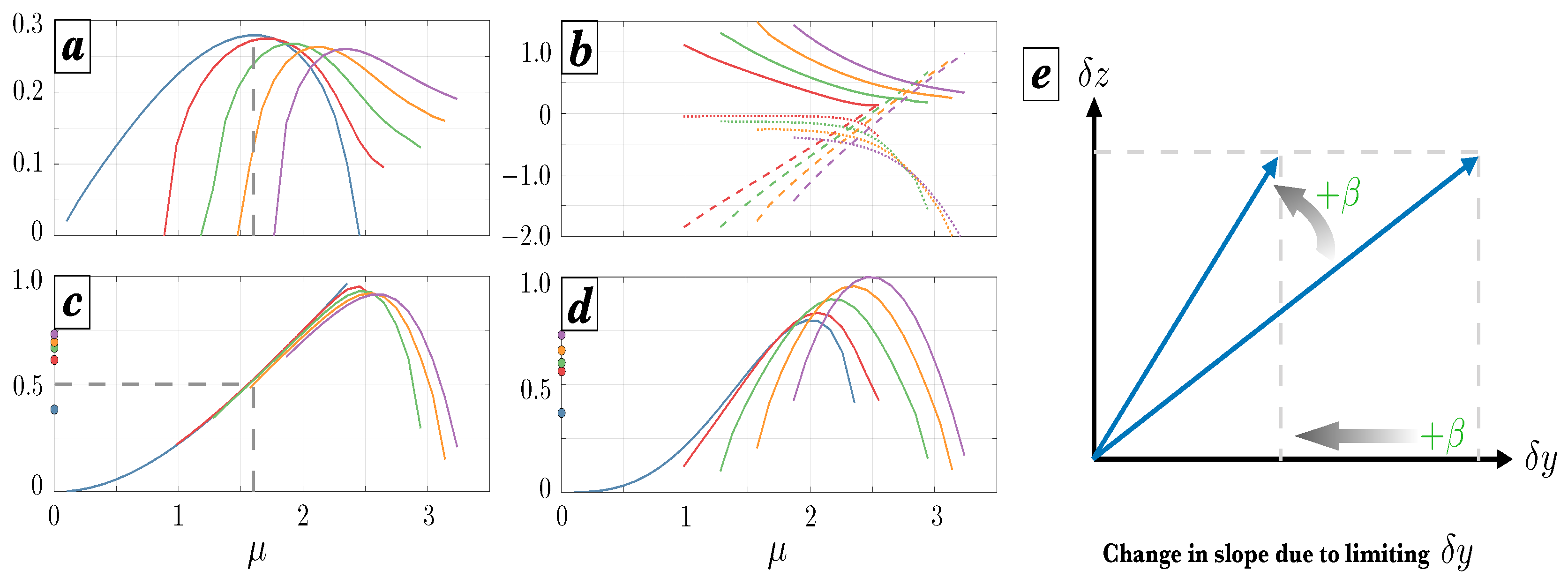
To investigate further, each output snapshot was Fourier transformed to obtain the values of each term in as a function of zonal (k) and meridional (l) wavenumber. Since the fastest growing mode in the linear instability problem corresponds to the gravest meridional mode, only the time-averaged results for are shown here. Figure 2a shows the diagnosed growth rates from layer 10, following the method described in (17) for calculating . The curve for the case, corresponding to the Eady model, matches the theory shown by [31], where the short-wave cutoff occurs at the normalized (nondimensional) wavenumber and maximal nondimensional growth rate occurs at . The curves for are shifted and tail off toward higher wavenumbers, akin to solutions of the Charney problem [40,41]; however, modes smaller than failed to demonstrate steady growth rates and featured erratic behavior of , and are thus excluded from this analysis.
Figure 2b shows the behavior of the terms in (16) as a function of . As predicted, the values of (solid lines) are always positive and become greater as increases. These curves bend upward toward smaller wavenumbers, unlike those of and , which appear to be constant and to trend linearly at small wavenumbers, respectively. Conversely, at large wavenumbers the effect of tends to zero, and the tendency for the slope to remain in the wedge of instability becomes a competition between (negative values) and (positive values). As shown in (14) the presence of the gradient operator in the numerator of suggests that this term should trend linearly with , which appears to be approximately the case for larger wavenumbers. Interestingly, transitions from negative to positive as one moves toward higher wavenumbers, with the transition point occurring near the short-wave cutoff for the Eady problem. Investigation of these behaviors at large wavenumbers are beyond the scope of this study, but are certainly worthy of further consideration.
Panel (c) shows values of as a function of , where the slope of the unstable modes essentially overlap each other regardless of the value of except at large wavenumbers. This suggests that near the deformation radius the slope of the modes becomes set by their physical size (i.e., distance of their meridional oscillations) rather than by . In the Eady case (blue line) where imposes no constraint, the slope of the modes transitions smoothly from the isopycnal slope () at small scales to horizontal () at the domain scale. The gray vertical dashed lines indicate the most unstable Eady mode at , at which conversion of EPE to eddy kinetic energy is maximized. This corresponds to the optimal buoyancy flux slope of (horizontal dashed line), affirming that energy conversion is maximized along the direction of the most unstable linear mode (e.g., [35]). This behavior stands in contrast to the cases , where because imposes a large-scale cutoff (panel a) the curves terminate at large scales with . Because the growth curves are shifted toward larger wavenumbers, the most unstable linear modes no longer correspond to the optimal slope ; rather, they occur at steeper slopes where potential energy conversion is less efficient.
Finally, these curves can be interpreted in the context of Figure 1a, which showed the domain-averaged values of calculated in physical space. The domain averaging essentially represents an average over all wavenumbers, but is weighted toward the more energetic, faster-growing modes. To this end, Figure 2d shows values of in panel (c) weighted by the growth rates in panel (a), and normalized so that the curve has a peak value of one. Here it is evident that the tendency for the growth curves to shift toward higher wavenumbers at larger means that the domain-averaged becomes weighted toward steeper modes.
In summary, the tendency for to increase with occurs because a nonzero imposes a threshold wavenumber above which the flow remains linearly stable. This prevents larger, shallower modes from contributing to the domain-averaged value of , and restricts instability to smaller waves which are less efficient at generating EPE (e.g., Appendix B in [42]). These small waves also are oriented at steeper slopes, further inhibiting EPE generation. A schematic depiction of this behavior is shown in Figure 2e. For a given vertical fluid parcel excursion , increasing restricts the horizontal distance the parcel can travel. The overall parcel trajectory thus becomes steeper, occurring along paths that are suboptimal for EPE generation. Even if the growth rates are not reduced significantly (panel a), limiting means that less EPE is generated overall irrespective of the trajectory. Together these effects can severely inhibit EPE generation (and thus eddy formation), possibly helping to explain observed “threshold behavior” (e.g., [33]) where the flow rapidly switches from eddy-dominated to jet-dominated states despite only small increases in the effective .
4. Conclusions
A useful mnemonic for teaching the concept of slope is “rise over run”, with the “rise” referring to the change in vertical position and the “run” referring to the change in horizontal position. The same mnemonic can be used to understand the effect of in inhibiting potential energy release by baroclinic instability. Two principle restoring forces exist in geophysical fluid dynamics: a vertical restoring force set by the density stratification that controls the “rise”, and a horizontal restoring force set by the potential vorticity gradient (a “half-cycle Coriolis force”, e.g., [43]) that controls the “run”. Thus, when is increased and the “run” is reduced, the slope of the eddy fluxes is increased.
The slope of the eddy fluxes depends on the horizontal wavelength, with larger waves naturally having shallower slopes and shorter waves steeper slopes. When the slopes within the range of unstable wavenumbers smoothly transition from the isopycnal slope at the short-wave cutoff to zero at the domain scale (Figure 2a, blue line). Thus, the set of unstable modes occupies the full extent of the wedge of instability. Nonzero restricts the unstable modes to a progressively smaller portion of this wedge; by imposing a long-wave cutoff, the eddy transport is forced to become steeper, inhibiting its ability to extract potential energy both by forcing it along suboptimal slopes and by limiting the distance of its horizontal excursions. This manifests in reduced linear growth rates and would likely imply a reduced ability to overcome the barotropic governor (e.g., [24]) and manifest baroclinic turbulence from a marginally stable barotropic jet.
This study focused on a relatively narrow portion of the baroclinic life cycle, namely the linear growth phase in the limit of constant . An interesting extension of these results might be found by exploring a flow configuration similar to that of [14], who found that linear growth rates increased with the strength of a spatially varying . Much of the theoretical framework introduced here would still apply when is nonconstant or even negative, albeit any expectations about its effects would have to be made depending on the specific flow configuration. It would be interesting to explore whether this theory has applications for flows where sloping bathymetry introduces an “effective ” and affects the instability of the baroclinic modes (e.g., [44]). It would likely be possible to apply some of the theory here to nonlinear or baroclinically adjusted flows as well (i.e., including jets or lateral shears) with appropriate modifications to the averaging, if necessary. These topics would make for interesting new perspectives on longstanding knowledge about -plane dynamics.
Supplementary Materials
The Dedalus and postprocessing scripts used in this manuscript are available online at https://github.com/sdbachman/Linearized-QG.
Funding
This research was funded by National Science Foundation grant number 1912420. This material is based on work supported by the National Center for Atmospheric Research (NCAR), which is a major facility sponsored by the National Science Foundation under Cooperative Agreement No. 1852977.
Acknowledgments
The author would like to thank John Taylor and Baylor Fox-Kemper for their excellent mentorship and encouragement in exploring this topic, and Jacob Wenegrat for designing the Dedalus script that was modified to conduct the simulations presented in this manuscript.
Conflicts of Interest
The author reports no conflict of interest.
References
- Dritschel, D.G.; McIntyre, M.E. Multiple jets as PV staircases: The Phillips effect and the resilience of eddy-transport barriers. J. Atmos. Sci. 2008, 65, 855–874. [Google Scholar] [CrossRef]
- Greenslade, M.D.; Haynes, P.H. Vertical transition in transport and mixing in baroclinic flows. J. Atmos. Sci. 2008, 65, 1137–1157. [Google Scholar] [CrossRef]
- Ferrari, R.; Nikurashin, M. Suppression of eddy diffusivity across jets in the Southern Ocean. J. Phys. Oceanogr. 2010, 40, 1501–1519. [Google Scholar] [CrossRef] [Green Version]
- Smith, K.S. Tracer transport along and across coherent jets in two-dimensional turbulent flow. J. Fluid Mech. 2005, 544, 133–142. [Google Scholar] [CrossRef] [Green Version]
- Rhines, P.B. Waves and turbulence on a beta-plane. J. Fluid Mech. 1975, 69, 417–443. [Google Scholar] [CrossRef] [Green Version]
- Sukoriansky, S.; Dikovskaya, N.; Galperin, B. On the arrest of inverse energy cascade and the Rhines scale. J. Atmos. Sci. 2007, 64, 3312–3327. [Google Scholar] [CrossRef]
- Dritschel, D.G.; Scott, R.K. Jet sharpening by turbulent mixing. Philos. Trans. R. Soc. A Math. Phys. Eng. Sci. 2011, 369, 754–770. [Google Scholar] [CrossRef]
- Williams, G.P. Planetary circulations: 1. Barotropic representation of Jovian and terrestrial turbulence. J. Atmos. Sci. 1978, 35, 1399–1426. [Google Scholar] [CrossRef] [Green Version]
- Lian, Y.; Showman, A.P. Deep jets on gas-giant planets. Icarus 2008, 194, 597–615. [Google Scholar] [CrossRef]
- Beron-Vera, F.J.; Brown, M.G.; Olascoaga, M.J.; Rypina, I.I.; Kocak, H.; Udovydchenkov, I.A. Zonal jets as transport barriers in planetary atmospheres. J. Atmos. Sci. 2008, 65, 3316–3326. [Google Scholar] [CrossRef]
- Berloff, P.; Kamenkovich, I.; Pedlosky, J. A mechanism of formation of multiple zonal jets in the oceans. J. Fluid Mech. 2009, 628, 395–425. [Google Scholar] [CrossRef] [Green Version]
- Peng, M.S.; Jeng, B.F.; Williams, R.T. A numerical study on tropical cyclone intensification. Part I: Beta effect and mean flow effect. J. Atmos. Sci. 1999, 56, 1404–1423. [Google Scholar] [CrossRef]
- Kidston, J.; Frierson, D.M.W.; Renwick, J.A.; Vallis, G.K. Observations, simulations, and dynamics of jet stream variability and annular modes. J. Clim. 2010, 23, 6186–6199. [Google Scholar] [CrossRef]
- Stamper, M.A.; Taylor, J.R.; Fox-Kemper, B. The growth and saturation of submesoscale instabilities in the presence of a barotropic jet. J. Phys. Oceanogr. 2018, 48, 2779–2797. [Google Scholar] [CrossRef]
- Galperin, B.; Sukoriansky, S.; Dikovskaya, N. Zonostrophic turbulence. Phys. Scr. 2008, 2008, 014034. [Google Scholar] [CrossRef]
- Galperin, B.; Sukoriansky, S.; Dikovskaya, N. Geophysical flows with anisotropic turbulence and dispersive waves: Flows with a β-effect. Ocean Dyn. 2010, 60, 427–441. [Google Scholar] [CrossRef]
- Farrell, B.F.; Ioannou, P.J. Structure and spacing of jets in barotropic turbulence. J. Atmos. Sci. 2007, 64, 3652–3665. [Google Scholar] [CrossRef]
- Srinivasan, K.; Young, W. Zonostrophic instability. J. Atmos. Sci. 2012, 69, 1633–1656. [Google Scholar] [CrossRef] [Green Version]
- Constantinou, N.C.; Farrell, B.F.; Ioannou, P.J. Emergence and equilibration of jets in beta-plane turbulence: Applications of stochastic structural stability theory. J. Atmos. Sci. 2014, 71, 1818–1842. [Google Scholar] [CrossRef] [Green Version]
- Tobias, S.; Marston, J. Direct statistical simulation of out-of-equilibrium jets. Phys. Rev. Lett. 2013, 110, 104502. [Google Scholar] [CrossRef] [Green Version]
- Bakas, N.A.; Ioannou, P.J. A theory for the emergence of coherent structures in beta-plane turbulence. J. Fluid Mech. 2014, 740, 312–341. [Google Scholar] [CrossRef] [Green Version]
- Bakas, N.A.; Constantinou, N.C.; Ioannou, P.J. S3T stability of the homogeneous state of barotropic beta-plane turbulence. J. Atmos. Sci. 2015, 72, 1689–1712. [Google Scholar] [CrossRef] [Green Version]
- Ioannou, P.; Lindzen, R.S. Baroclinic instability in the presence of barotropic jets. J. Atmos. Sci. 1986, 43, 2999–3014. [Google Scholar] [CrossRef]
- James, I.N. Suppression of baroclinic instability in horizontally sheared flows. J. Atmos. Sci. 1987, 44, 3710–3720. [Google Scholar] [CrossRef] [Green Version]
- Nakamura, N. An illustrative model of instabilities in meridionally and vertically sheared flows. J. Atmos. Sci. 1993, 50, 357–376. [Google Scholar] [CrossRef] [Green Version]
- Panetta, R.L. Zonal jets in wide baroclinically unstable regions: Persistence and scale selection. J. Atmos. Sci. 1993, 50, 2073–2106. [Google Scholar] [CrossRef] [Green Version]
- Taylor, J.R.; Bachman, S.D.; Stamper, M.A.; Hosegood, P.; Adams, K.; Sallee, J.B.; Torres, R. Submesoscale Rossby waves on the Antarctic Circumpolar Current. Sci. Adv. 2018, 4, eaao2824. [Google Scholar] [CrossRef] [Green Version]
- Nakamura, N. Momentum flux, flow symmetry, and the nonlinear barotropic governor. J. Atmos. Sci. 1993, 50, 2159–2179. [Google Scholar] [CrossRef]
- Green, J.S.A. A problem in baroclinic stability. Q. J. R. Meteorol. Soc. 1960, 86, 237–251. [Google Scholar] [CrossRef]
- Lindzen, R.S. The Eady problem for a basic state with zero PV gradient but β ≠ 0. J. Atmos. Sci. 1994, 51, 3221–3226. [Google Scholar] [CrossRef]
- Vallis, G.K. Atmospheric and Oceanic Fluid Dynamics; Cambridge University Press: Cambridge, UK, 2017. [Google Scholar]
- Farrell, B.F.; Ioannou, P.J. Formation of jets by baroclinic turbulence. J. Atmos. Sci. 2008, 65, 3353–3375. [Google Scholar] [CrossRef] [Green Version]
- Klocker, A. Opening the window to the Southern Ocean: The role of jet dynamics. Sci. Adv. 2018, 4, eaao4719. [Google Scholar] [CrossRef] [Green Version]
- Eady, E.T. Long waves and cyclone waves. Tellus 1949, 1, 33–52. [Google Scholar] [CrossRef] [Green Version]
- Thorpe, A.J.; Hoskins, B.J.; Innocentini, V. The parcel method in a baroclinic atmosphere. J. Atmos. Sci. 1989, 46, 1274–1284. [Google Scholar] [CrossRef] [Green Version]
- Taylor, J.R.; Ferrari, R. Buoyancy and wind-driven convection at mixed layer density fronts. J. Phys. Oceanogr. 2010, 40, 1222–1242. [Google Scholar] [CrossRef] [Green Version]
- Heifetz, E.; Alpert, P.; Da Silva, A. On the parcel method and the baroclinic wedge of instability. J. Atmos. Sci. 1998, 55, 788–795. [Google Scholar] [CrossRef]
- Maddison, J.; Marshall, D. The Eliassen-Palm flux tensor. J. Fluid Mech. 2013, 729, 69. [Google Scholar] [CrossRef]
- Burns, K.J.; Vasil, G.M.; Oishi, J.S.; Lecoanet, D.; Brown, B.P. Dedalus: A flexible framework for numerical simulations with spectral methods. Phys. Rev. Res. 2020, 2, 023068. [Google Scholar] [CrossRef] [Green Version]
- Charney, J.G. The dynamics of long waves in a baroclinic westerly current. J. Meteorol. 1947, 4, 136–162. [Google Scholar] [CrossRef]
- Kuo, H.L. Baroclinic instabilities of linear and jet profiles in the atmosphere. J. Atmos. Sci. 1979, 36, 2360–2378. [Google Scholar] [CrossRef] [Green Version]
- Haine, T.W.N.; Marshall, J. Gravitational, symmetric, and baroclinic instability of the ocean mixed layer. J. Phys. Oceanogr. 1998, 28, 634–658. [Google Scholar] [CrossRef]
- Cai, M.; Huang, B. A new look at the physics of Rossby waves: A mechanical–Coriolis oscillation. J. Atmos. Sci. 2013, 70, 303–316. [Google Scholar] [CrossRef]
- Blumsack, S.L.; Gierasch, P. Mars: The effects of topography on baroclinic instability. J. Atmos. Sci. 1972, 29, 1081–1089. [Google Scholar] [CrossRef] [Green Version]
Figure 1.
Values of (a) , (b) , and (c) the component terms of in (16), across the interior model layers. Mean values for each curve are shown by the dots on the left side of each panel.
Figure 1.
Values of (a) , (b) , and (c) the component terms of in (16), across the interior model layers. Mean values for each curve are shown by the dots on the left side of each panel.

Figure 2.
(a) Diagnosed growth rates, (b) behavior of the terms in (16), (c) values of , and (d) values of weighted by growth rate, as functions of the nondimensional wavenumber . The gray dashed lines indicate the most unstable Eady wave at . The legend for these plots is the same as in Figure 1. (e) Schematic showing the steepening of the buoyancy flux slope when meridional parcel excursions are limited as increases.

© 2020 by the author. Licensee MDPI, Basel, Switzerland. This article is an open access article distributed under the terms and conditions of the Creative Commons Attribution (CC BY) license (http://creativecommons.org/licenses/by/4.0/).
Share and Cite
MDPI and ACS Style
Bachman, S.D. A Geometric Perspective on the Modulation of Potential Energy Release by a Lateral Potential Vorticity Gradient. Fluids 2020, 5, 142. https://0-doi-org.brum.beds.ac.uk/10.3390/fluids5030142
AMA Style
Bachman SD. A Geometric Perspective on the Modulation of Potential Energy Release by a Lateral Potential Vorticity Gradient. Fluids. 2020; 5(3):142. https://0-doi-org.brum.beds.ac.uk/10.3390/fluids5030142
Chicago/Turabian StyleBachman, Scott D. 2020. "A Geometric Perspective on the Modulation of Potential Energy Release by a Lateral Potential Vorticity Gradient" Fluids 5, no. 3: 142. https://0-doi-org.brum.beds.ac.uk/10.3390/fluids5030142