1. Introduction
The large skin-friction drag characterizing wall-bounded turbulent flows, as compared to laminar ones, represents a major challenge in engineering applications where efficiency and running costs of fluid transport systems are of interest. This has motivated several experimental and numerical studies aimed at a better understanding of the phenomenon of turbulence production and generation of Reynolds shear stress in such flows [
1,
2,
3,
4]; the coherent structures in the inner region of the wall layer and the
bursting (ejection) and
sweep (inrush) events related to such structures have been the object of intense research activities [
5,
6,
7,
8]. The design of active or passive techniques for turbulent drag reduction requires in-depth understanding of the interacting mechanisms which contribute to near-wall turbulence, in order for its effective control. The near-wall flow is characterized by a self-sustaining cycle responsible for the regeneration of turbulent fluctuations, owing to the dynamic interaction between longitudinal velocity streaks and quasi-streamwise vortices; this cycle is independent of the nature of the outer flow [
9]. Attenuating (or suppressing) any of the processes involved in this autonomous cycle can lead to a less disturbed flow field (or even to relaminarization) [
9], a clear advantage when the objective of the control is skin-friction drag.
Many investigations have been conducted to optimize and assess the effectiveness and feasibility of active and passive drag reduction techniques, to favorably alter the structure of the turbulent boundary layer. Active techniques, involving energy input, have proved to yield significant drag reduction in wall-bounded turbulent flows. For instance, optimized uniform blowing of the fluid through a spanwise slot can produce a local drag reduction of
downstream of the slot [
10], while sufficiently high suction rates through a short porous flush-mounted strip can allow for local relaminarization of the turbulent boundary layer, resulting in a drag reduction of more than
[
11]. Counter-rotating large-scale streamwise vortices, externally initiated by a transverse array of longitudinal plasma actuators, can stabilize the streaks in the near-wall flow and attenuate the coherent structures, interrupting the turbulence regeneration cycle; a drag reduction of more than
can be achieved [
12,
13]. Other studies focused on forcing wall-normal fluctuations [
14] or in-plane wall oscillations [
15,
16]. Passive drag reduction techniques have also been investigated extensively, along with remarkable advances in bio-inspired designs. Riblets (longitudinal surface grooves) have proved to mitigate the velocity fluctuations near the wall, resulting in a more uniform flow field [
17]; studies on different configurations of riblets revealed that an optimized drag reduction of almost
can be achieved [
18]. Super-hydrophobic surfaces can reduce drag up to approximately
under optimal conditions, mainly due to the large effective slip of aqueous solutions on the walls [
19]. The ability of anisotropic permeable substrates to reduce skin-friction drag in turbulent channel flows has recently attracted much interest; this constitutes the main objective of the present study.
Porous substrates are encountered in various natural and engineering applications, and have been a source of inspiration for many studies in which the influence of wall permeability has been assessed on the behavior of the overlying turbulent boundary layer and ensuing drag alteration. Several configurations of the porous substrate have been investigated, with different values of the porosity (
) and at different flow conditions. The main parameters tested in previous studies are the diagonal components of the permeability tensor of the porous medium (
,
,
) and the Navier-slip coefficients (
,
) at the dividing surface between the free-fluid region in the channel and the permeable layer. In the following,
x,
y and
z denote, respectively, the streamwise, wall-normal and spanwise directions. The numerical work by Rosti et al. [
20] on turbulent channel flows over isotropic porous substrates (
) has shown that even small values of the medium permeability can affect the response of the adjacent turbulent boundary layer: the disturbances were found to be intensified and the Reynolds stresses enhanced, with a consequent increase in skin-friction drag. This is in general agreement with the findings of earlier studies [
21,
22,
23]. A similar behavior of disturbance intensification is observed when the porous substrates have preferential spanwise permeability. Wang et al. [
24] investigated the dynamic interaction between a turbulent channel flow and a porous bed made of spanwise-aligned cylinders, for which
. The structure of the
blowing (upwelling) and
suction (downwelling) events through the pores has been analyzed, particularly in terms of their role on the onset of the Kelvin–Helmholtz instability near the permeable wall. Other studies have focused on permeable walls potentially capable to yield turbulent drag reduction. Rosti et al. [
25] studied the turbulent flow over anisotropic porous beds characterized by equal values of the permeability in the streamwise and the spanwise directions, i.e.,
. They showed that a drag reduction of up to 20% can be achieved from walls of high in-plane permeability (
), whereas the skin-friction drag may increase by the same amount for substrates of preferential wall-normal permeability. Among the different configurations considered in the literature, the use of porous substrates of preferential permeability along the streamwise direction, consisting, e.g., of longitudinal cylinders with
, appears to provide the best results in terms of turbulent drag reduction. The drag reduction curves for this configuration are similar to those of riblets [
26], and the theory behind the ability of such substrates to reduce skin-friction drag has been elaborated by Abderrahaman-Elena and García-Mayoral [
27]. Conceptually, the drag reduction (
) is proportional to the difference between the slip lengths along the streamwise and the spanwise directions, that is,
[
28,
29], which has been approximated by
[
27]. All the macroscopic parameters are measured in wall units and this is indicated by the superscript ‘+’; the coefficient
is a function of the Reynolds number [
30], while the parameter
characterizes the inter-connectivity of the flow between the pores [
27]. The relation above in terms of the square root of the permeability components holds for substrates of relatively low wall-normal permeability; if
exceeds some critical threshold, Kelvin–Helmholtz-like rollers are developed near the interface, and the drag reduction mechanism is adversely affected [
31].
With the significant progress in manufacturing and fabrication techniques, the study of the interaction between the microscale features of the surface (such as roughness, porosity, irregularity, compliance, etc.) and the adjacent fluid flow has become more important for several applications. The numerical complexity of fully resolving the micro-details of the surface in Direct Numerical Simulations (DNS) or even in Large Eddy Simulations (LES) of turbulence represents a challenge, especially if optimization of the surface is the ultimate goal. The multiscale homogenization approach adopted in this paper is a mathematical framework through which the rapidly varying properties of the surface (the porous substrate in the present case) can be replaced by upscaled properties such as slip, interface permeability, etc. [
32,
33], which contribute to the definition of
effective boundary conditions at a virtual plane surface. The macroscale behavior of, for instance, the turbulent channel flow is then targeted, bypassing the need to fully resolve the motion within the permeable substrate; the mesh requirements of the numerical simulations are therefore significantly alleviated. Multiscale homogenization has been known and used by applied mathematicians for a long time. In more recent years, it has been rediscovered and applied to a variety of physically relevant cases. Although the classical first-order slip condition over a generic solid surface, proposed by Navier [
34], was based on empirical considerations concerning the near-wall flow behavior, recent studies adopting the homogenization technique have provided a robust mathematical framework for the estimation of Navier’s slip length,
, without the need for any ad hoc correlation [
35]. A tensorial generalization of the first-order Navier’s slip condition over a micro-textured surface was given by Zampogna et al. [
36], via the definition of a third-order slip tensor which depends on the geometry of the roughness pattern. The homogenized model was later extended to study the fluid motion over deformable riblets, to assess the potential drag reduction [
37]. The so-called
transpiration-resistance model by Lācis et al. [
38] shed light on the role of the wall-normal velocity at the fictitious interface in improving the predictions of the homogenization-based direct simulations for turbulent flows over micro-patterned surfaces. The homogenization model for the flow over a rough surface was later pushed to third-order in terms of a small parameter, ratio of microscopic to macroscopic length scales, by Bottaro and Naqvi [
39]. Most recently, the asymptotic homogenization theory has been employed by Ahmed et al. [
40] to study buoyancy-driven flows over vertical rough surfaces, by deriving and implementing upscaled velocity and temperature boundary conditions at a smooth virtual surface. Effective boundary conditions at the interface between a porous bed and an unconfined flow region have been explored by Sudhakar et al. [
41] and by Naqvi and Bottaro [
42].
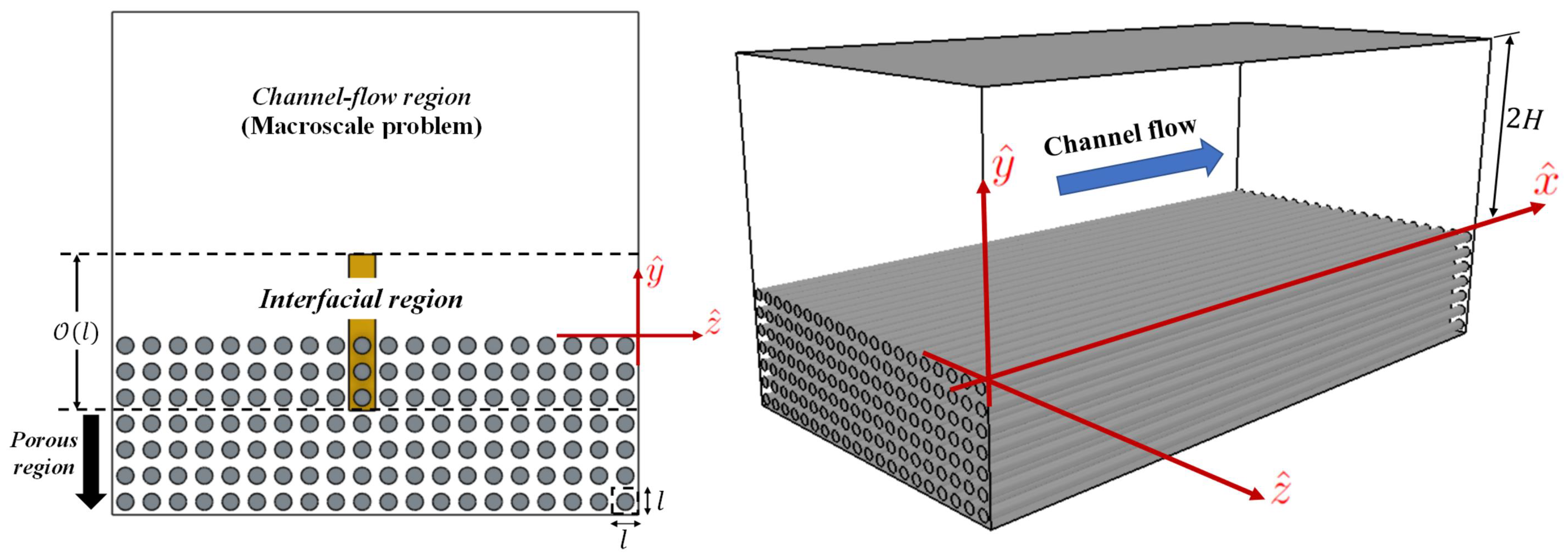
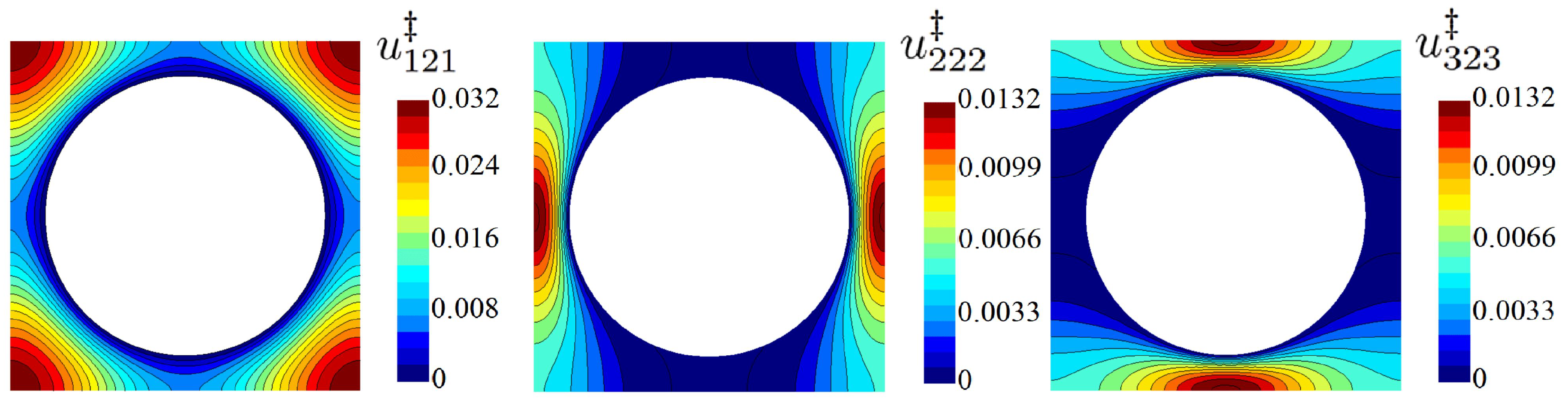
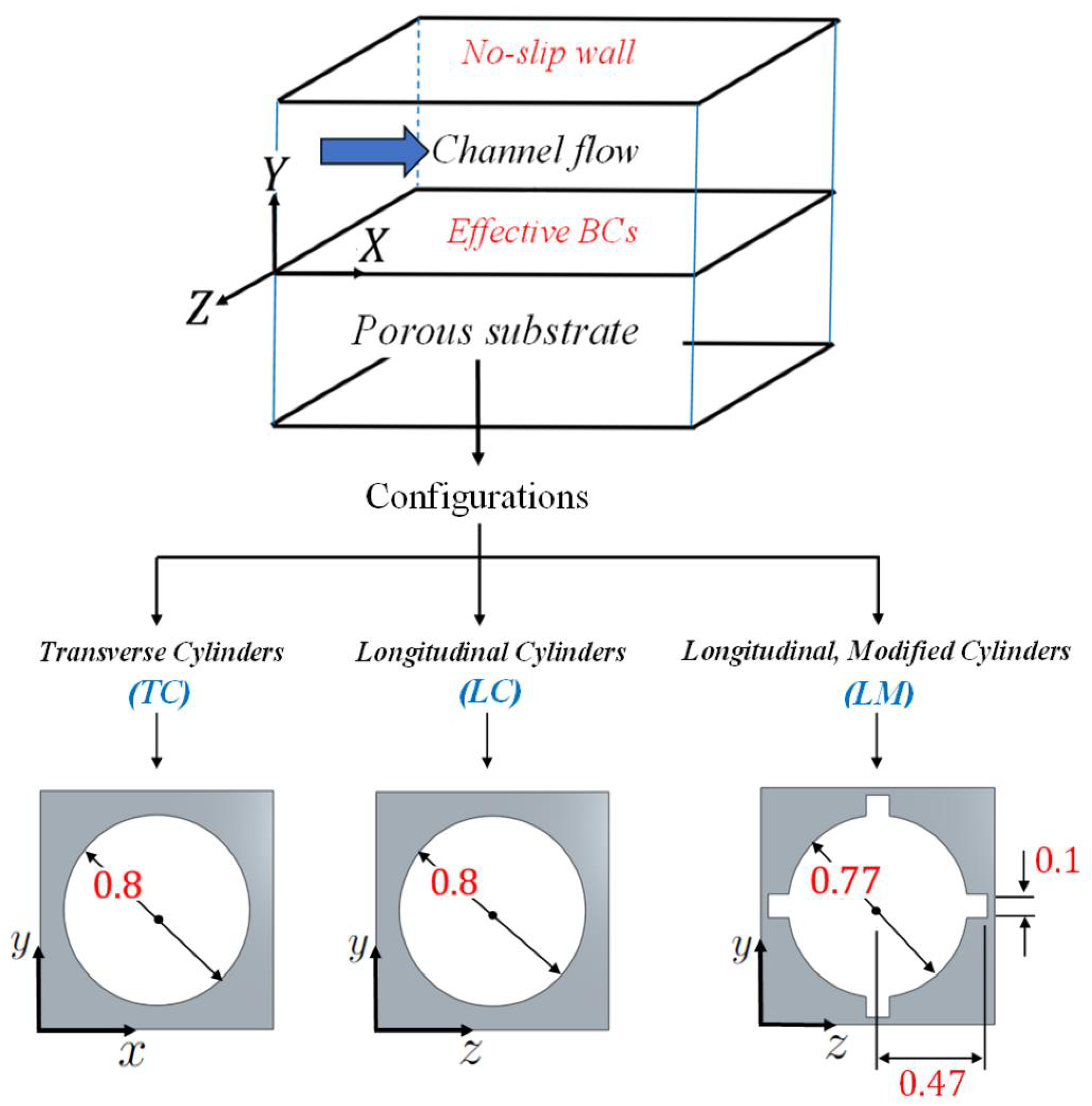
In this work, asymptotic homogenization is used to derive second-order accurate
effective boundary conditions for the three velocity components at a fictitious interface, chosen tangent to the porous material, to macroscopically mimic the effects of the small-scale features of an anisotropic porous layer on a turbulent boundary layer. The technique relies on reconstructing the microscale problem via asymptotic expansions of the microscopic dependent variables (velocity components and pressure) in powers of a small parameter
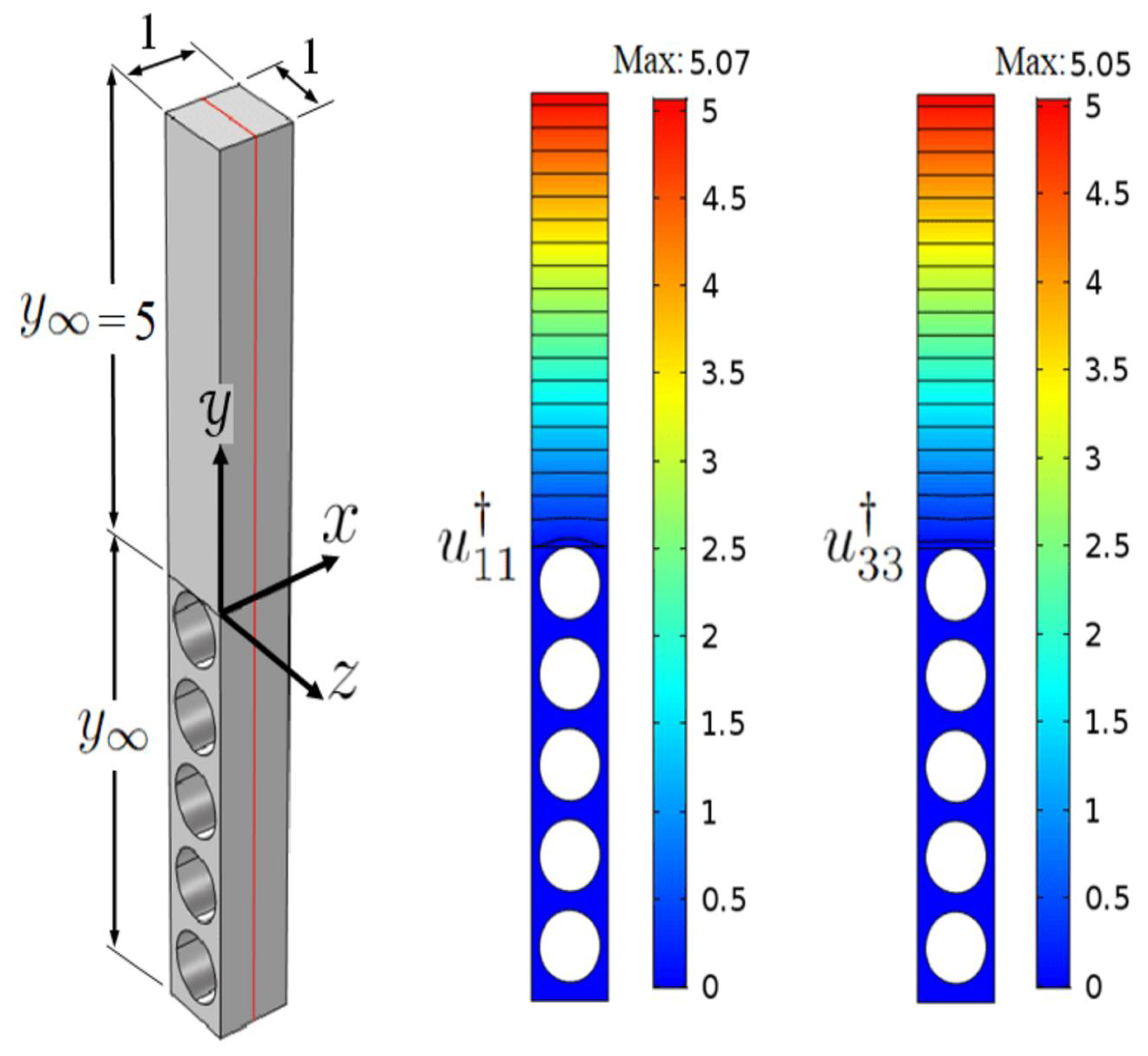
, which represents the ratio between two well-separated scales, for instance the periodicity of the porous pattern (microscopic length scale) and half the channel height (macroscopic length scale). The problem is then solved up to any order in
via numerical solution of ad hoc auxiliary systems which hold in a doubly periodic
representative elementary volume. The equations governing the physical problem, the domain decomposition, and the chosen scales for each sub-domain are outlined in
Section 2, with detailed explanation of the adopted asymptotic approach and with illustration of the numerical solutions for the auxiliary problems that arise. Different configurations of the porous substrate are considered for the evaluation of the macroscopic coefficients of the model, in particular, spanwise- and streamwise-aligned elements of two different shapes.The macroscopic problem is addressed in
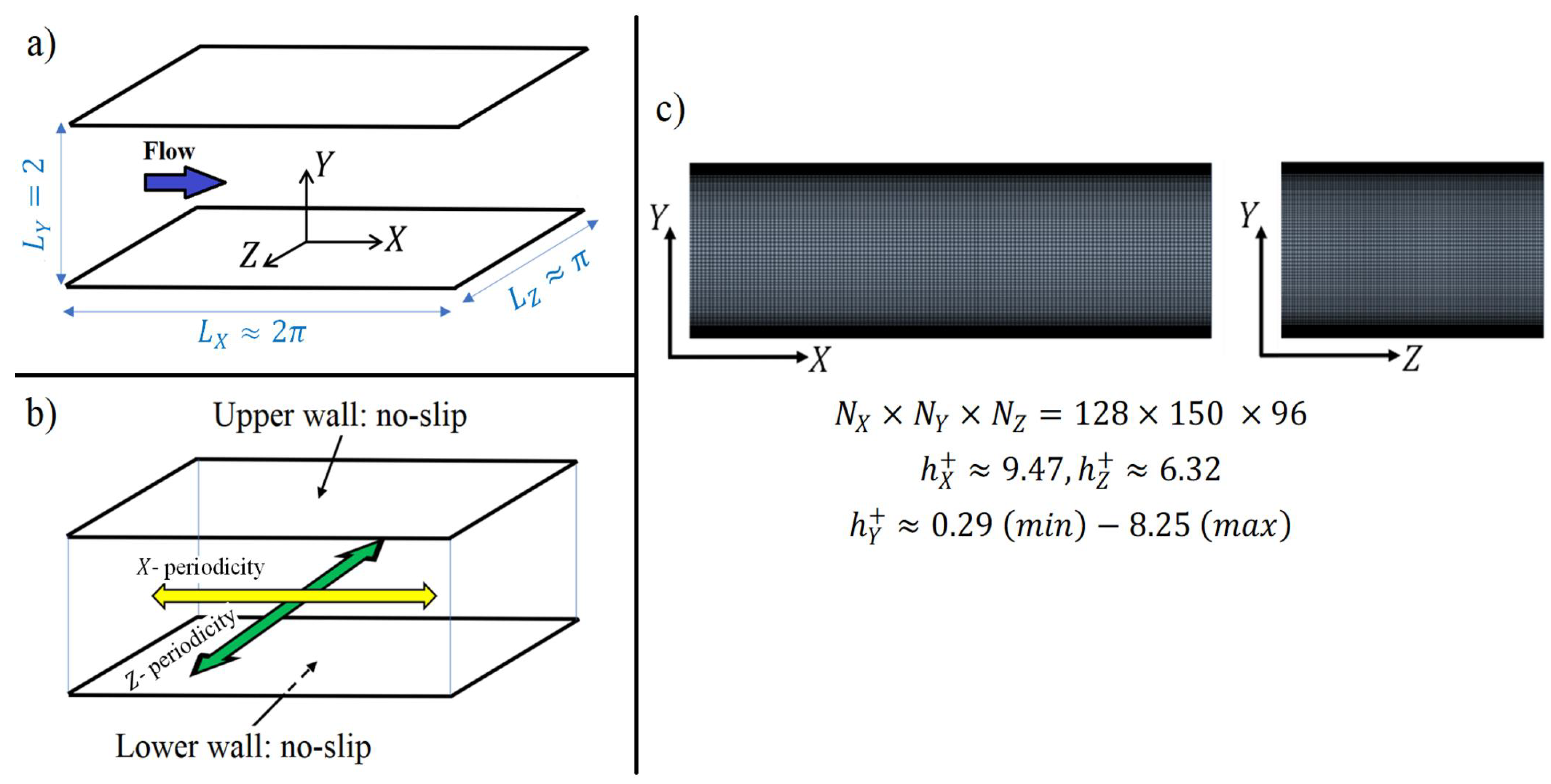
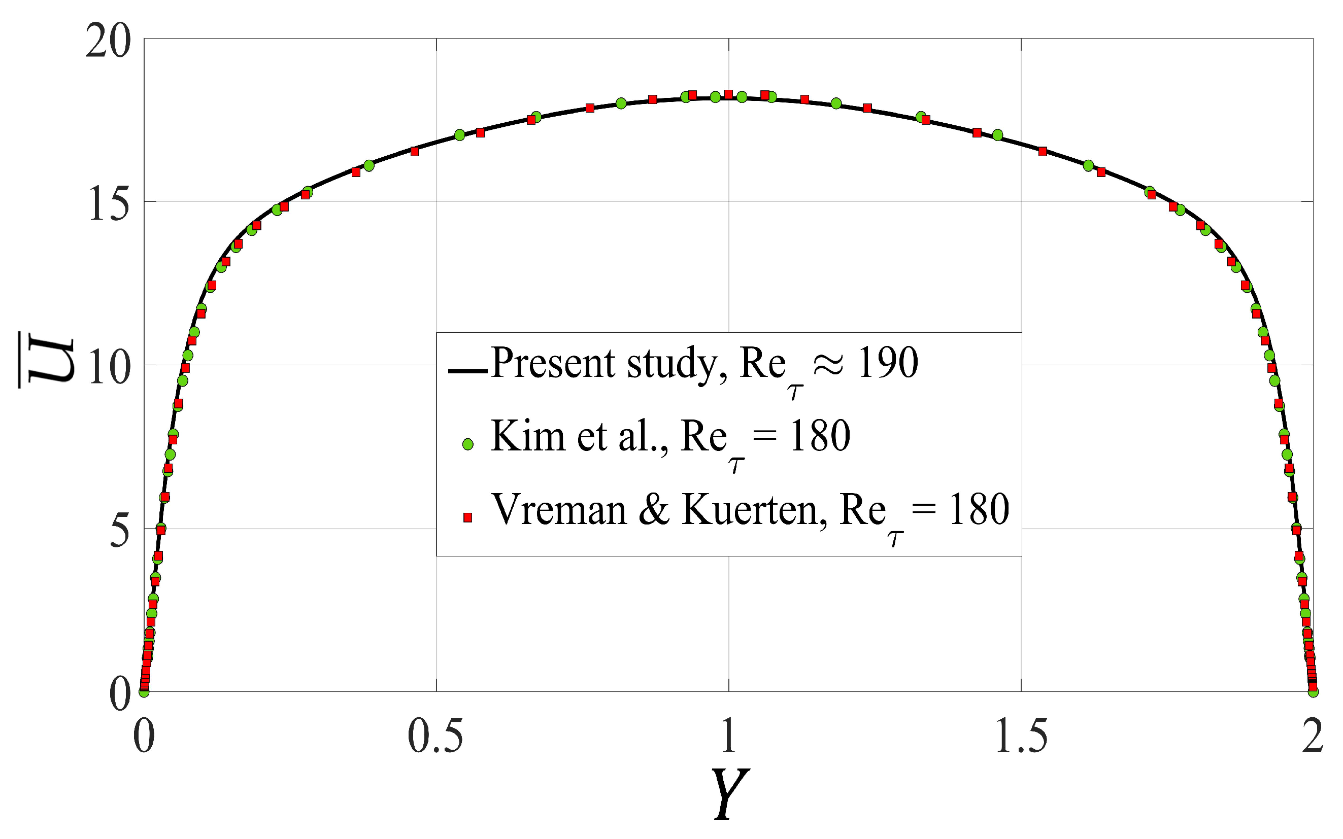
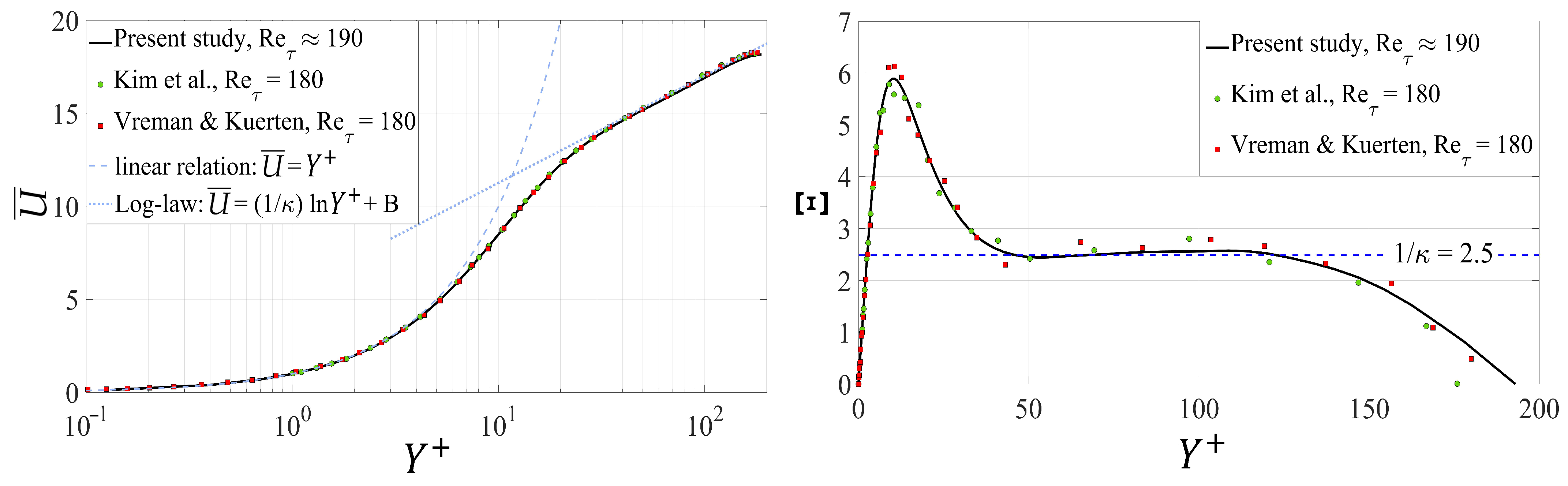
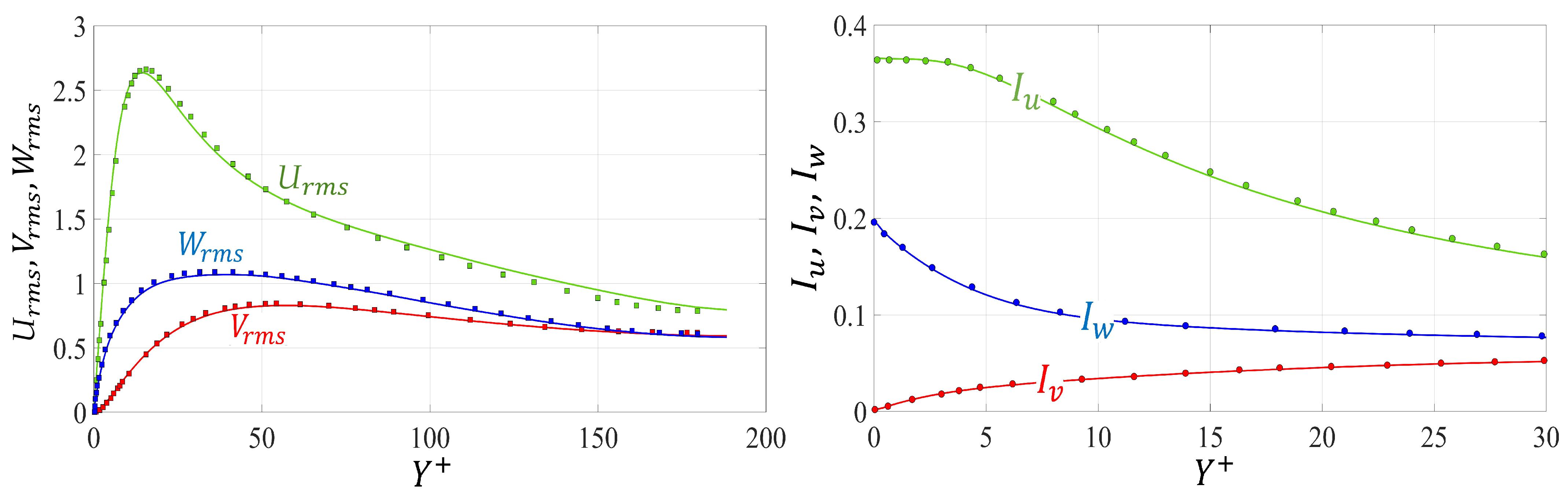
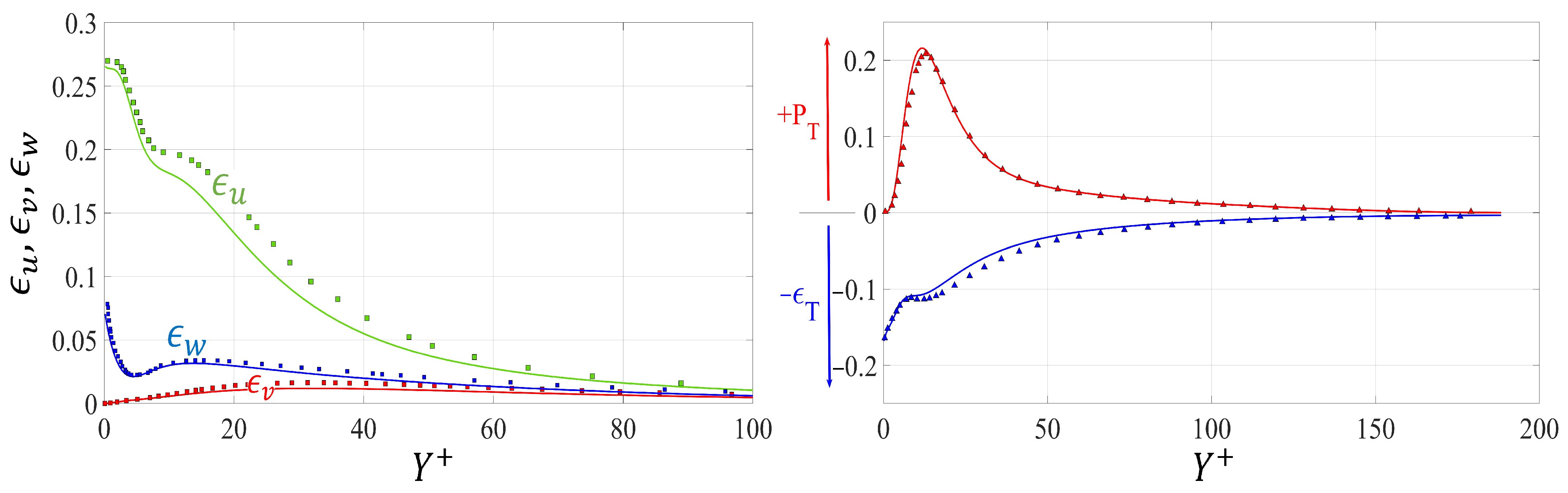
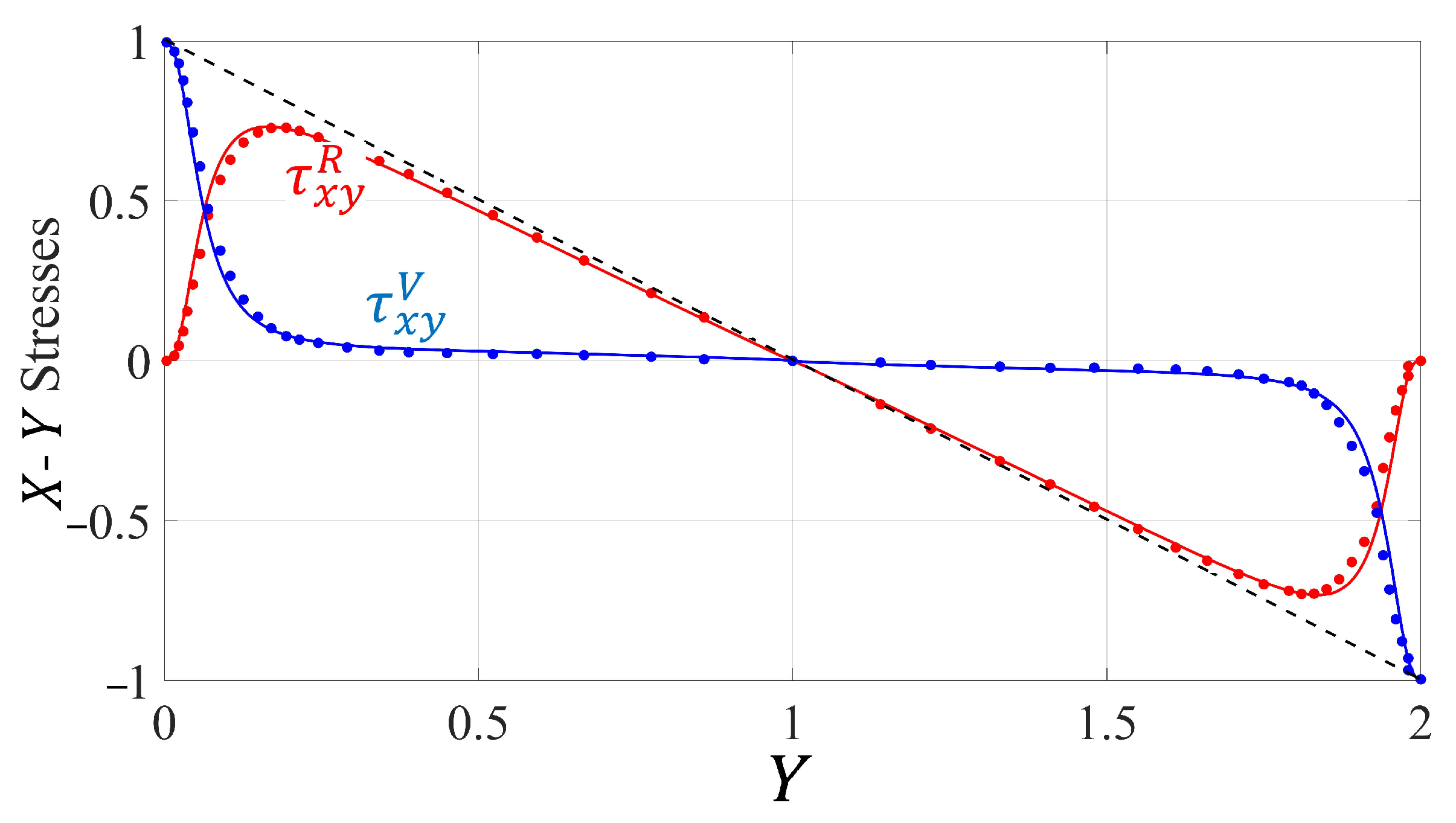
Section 3. A direct numerical simulation was first conducted for a turbulent flow through a channel with smooth, impermeable walls at
, to validate the numerical code, the domain size, etc. The wall-bounded turbulent flow over a porous substrate is then considered. Standard turbulence statistics are compared for different porous substrates, and consequent skin-friction drag increase/reduction is indicated. The main findings of the study are highlighted in the concluding section.
4. Conclusions
The high skin-friction drag characterizing wall-bounded turbulent flows adversely affects the efficiency of fluid transportation systems. It is thus important to develop effective drag reduction strategies, e.g., properly engineered passive flow control surfaces/substrates. In the present work, turbulent channel flows over transversely isotropic permeable beds of different types were numerically studied, and the consequent favorable/adverse changes in the skin-friction drag coefficient were monitored and described by analyzing turbulence statistics.
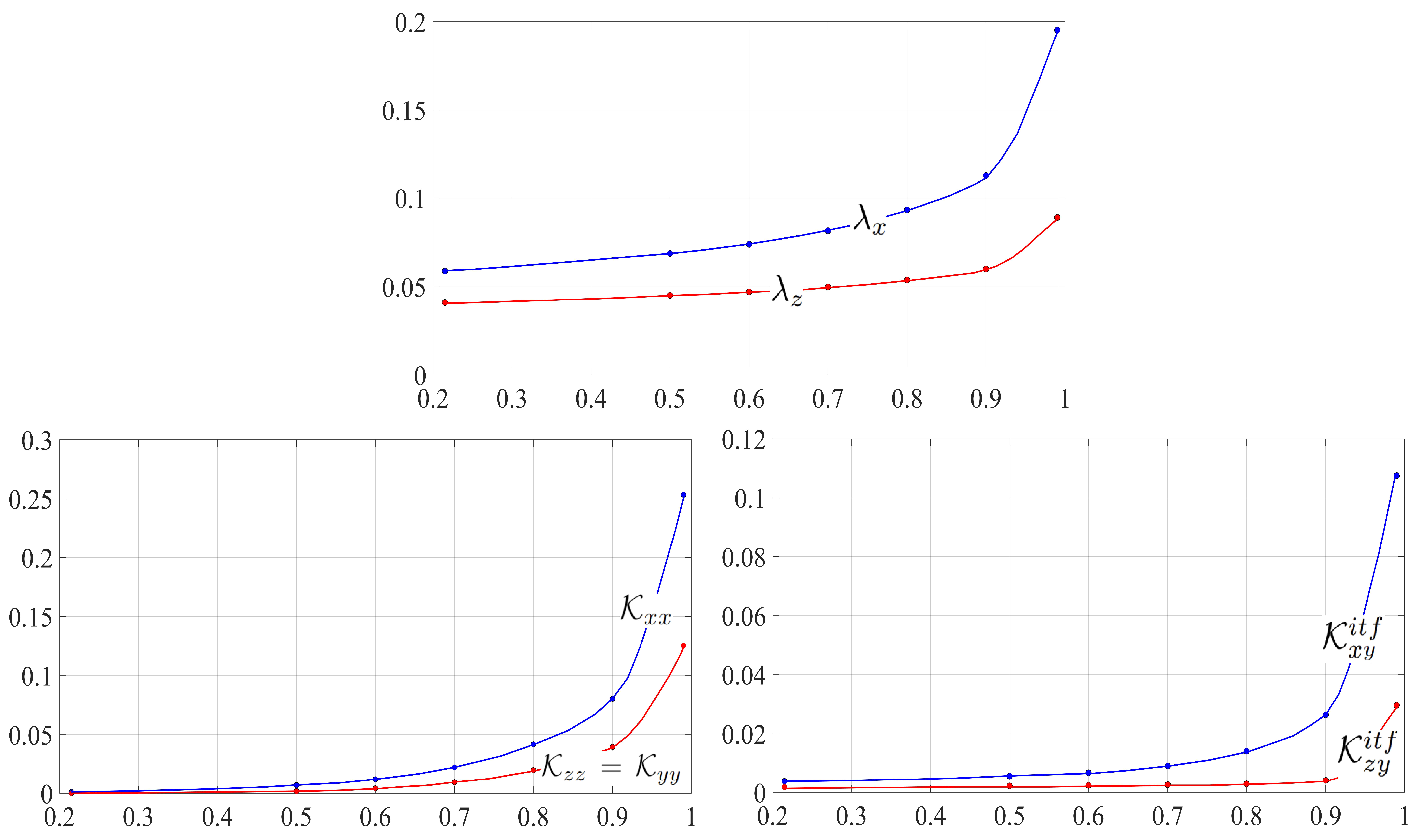
A multiscale homogenization approach was introduced to avoid the numerical complexity and the expensive mesh requirements of a full resolution of the flow within the porous media. Expressions for the effective boundary conditions of the three velocity components were sought at a fictitious interface between the channel flow and the porous bed, up to second-order accuracy in terms of a small parameter . The upscaled coefficients appearing in the definition of the effective boundary conditions, i.e., the slip lengths (), the medium permeability in the wall-normal direction () and the interfacial permeabilities (), were numerically calculated for three microstructures of the porous substrate. In particular, the microstructures considered were: () transverse, Z-aligned, plain cylinders; () longitudinal, X-aligned plain cylinders; () longitudinal, X-aligned, cylinders modified by the addition of four fins on the circumference, especially designed to amplify the quantity () while reducing the medium permeability, .
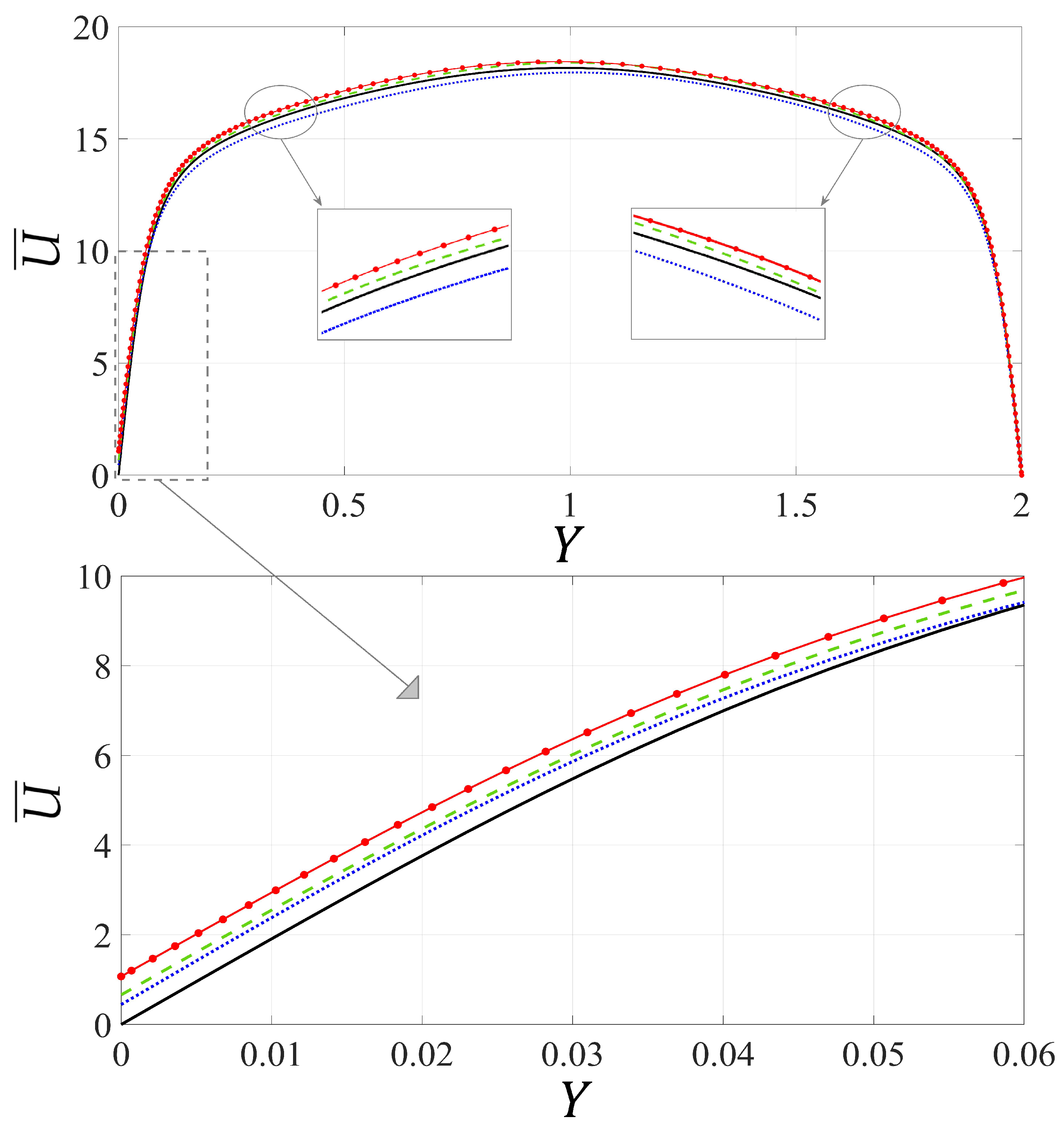
Direct numerical simulations of the macroscale problem above the virtual interface with the different porous beds have been conducted, employing the finite volume method with the Hybrid MUSCL 3rd-order/central-differencing discretization scheme, initially validated on the flow through a smooth channel. A value of was first employed, in order to focus on relatively small surface protrusions; the flow over the substrates , and was numerically studied, and the turbulence statistics were analyzed in detail. Secondly, the value of was increased to for the substrates , , and the consequent changes in the skin-friction drag coefficient and other flow metrics of interest were examined. Clearly, the gauge factor cannot be increased too much for the asymptotic expansion to remain valid. The range of validity of the approach, in terms of acceptable values of , will be investigated in future work. The major findings of the present study are summarized below:
- (i)
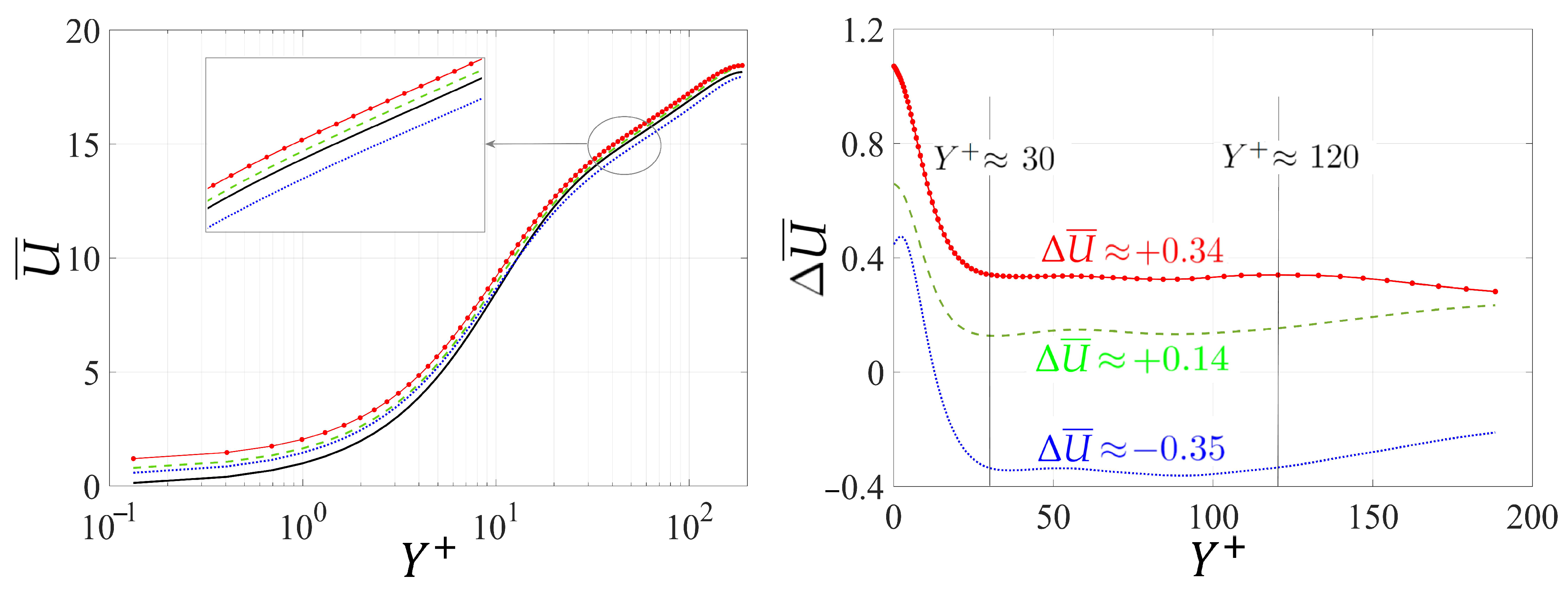
The permeable substrates with preferential slip in the streamwise direction (
), i.e., those designed with longitudinal (either plain or modified) cylinders, are able to reduce skin-friction drag. This conclusion should hold up to some critical value of
at which large-scale instabilities have their onset in the near-wall layer [
31].
- (ii)
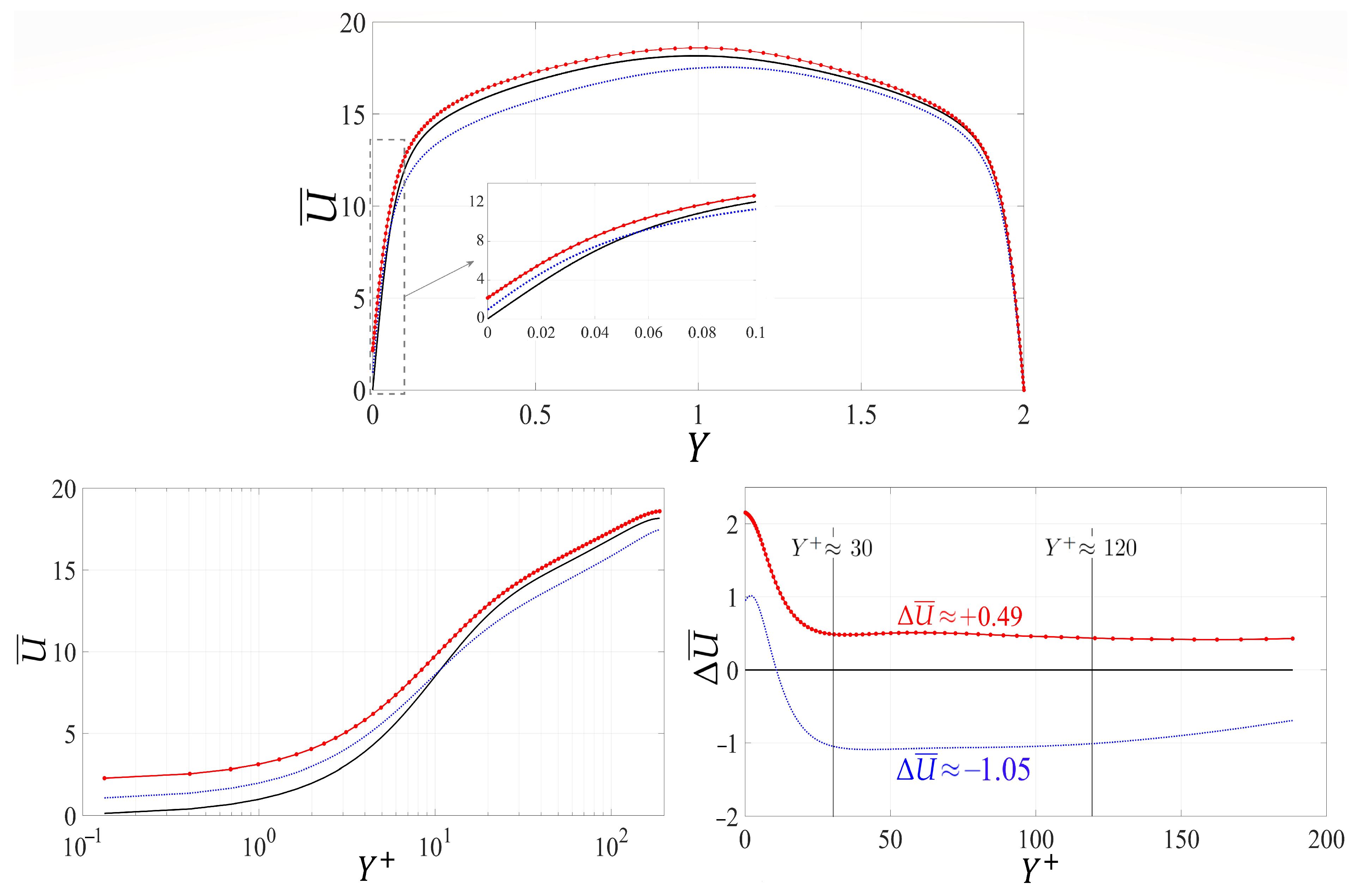
The adverse/favorable changes in the skin-friction drag coefficient are more pronounced for the substrates with . The drag coefficient increases by almost with the substrate , while about drag reduction is obtained with the substrate .
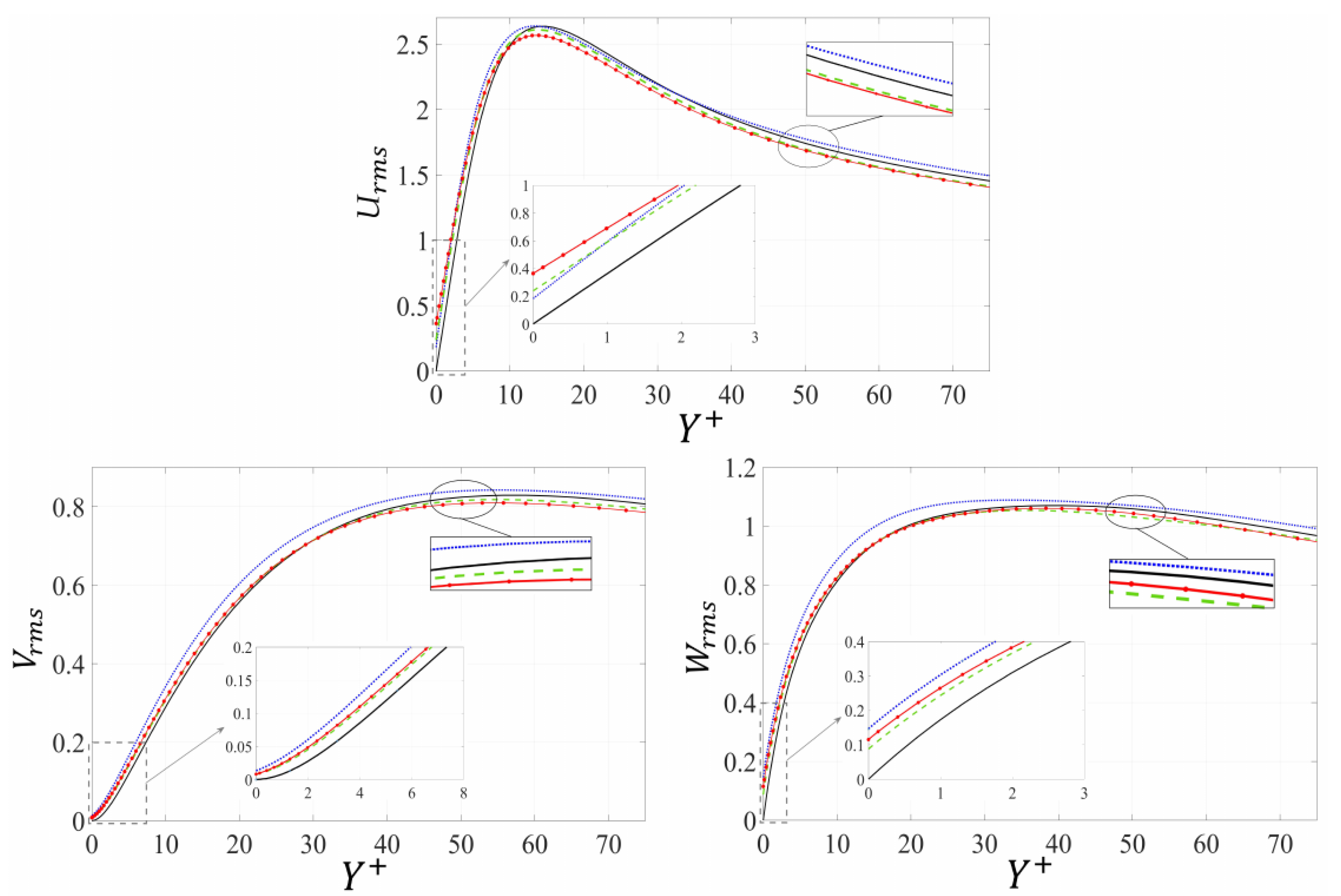
- (iii)
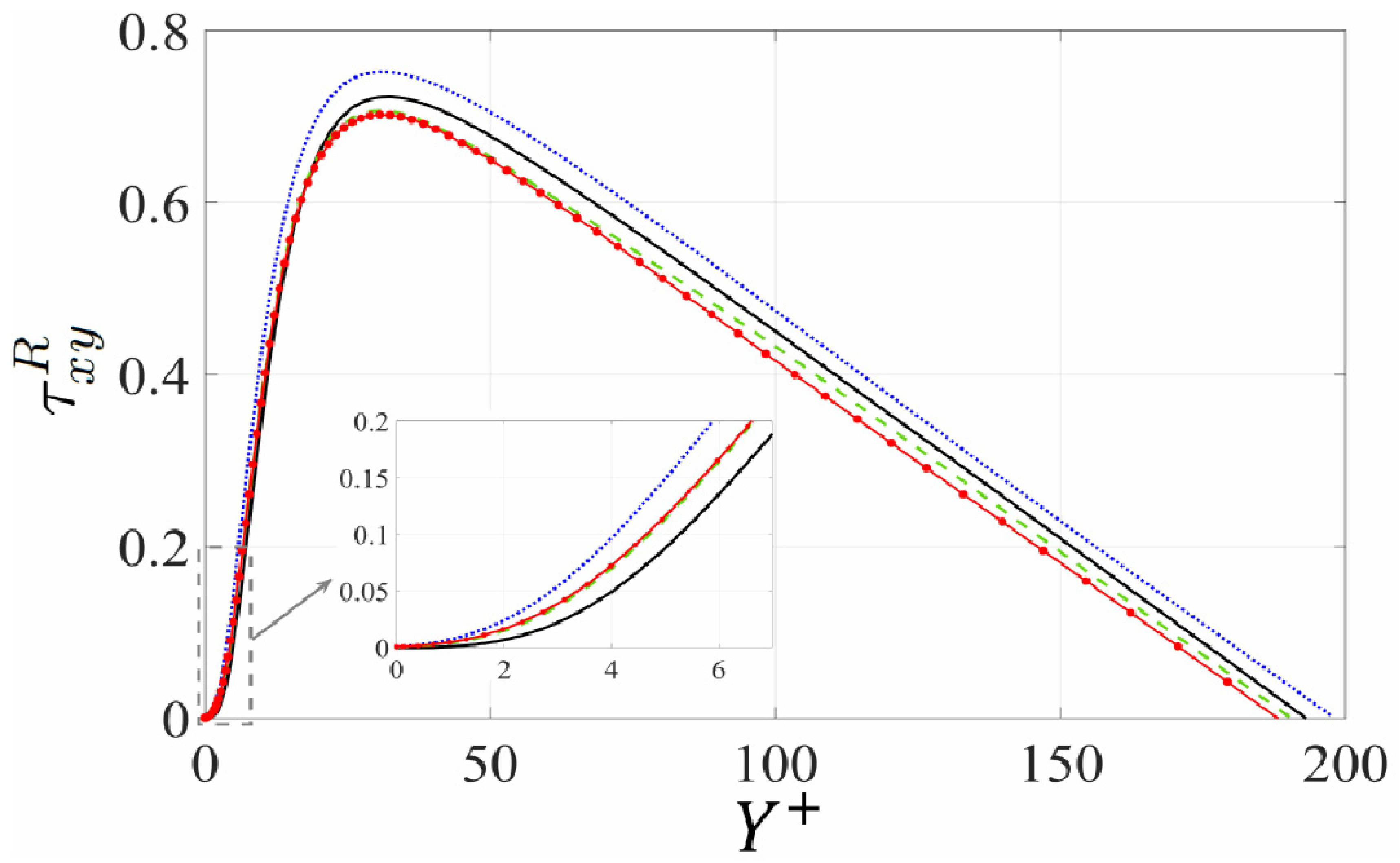
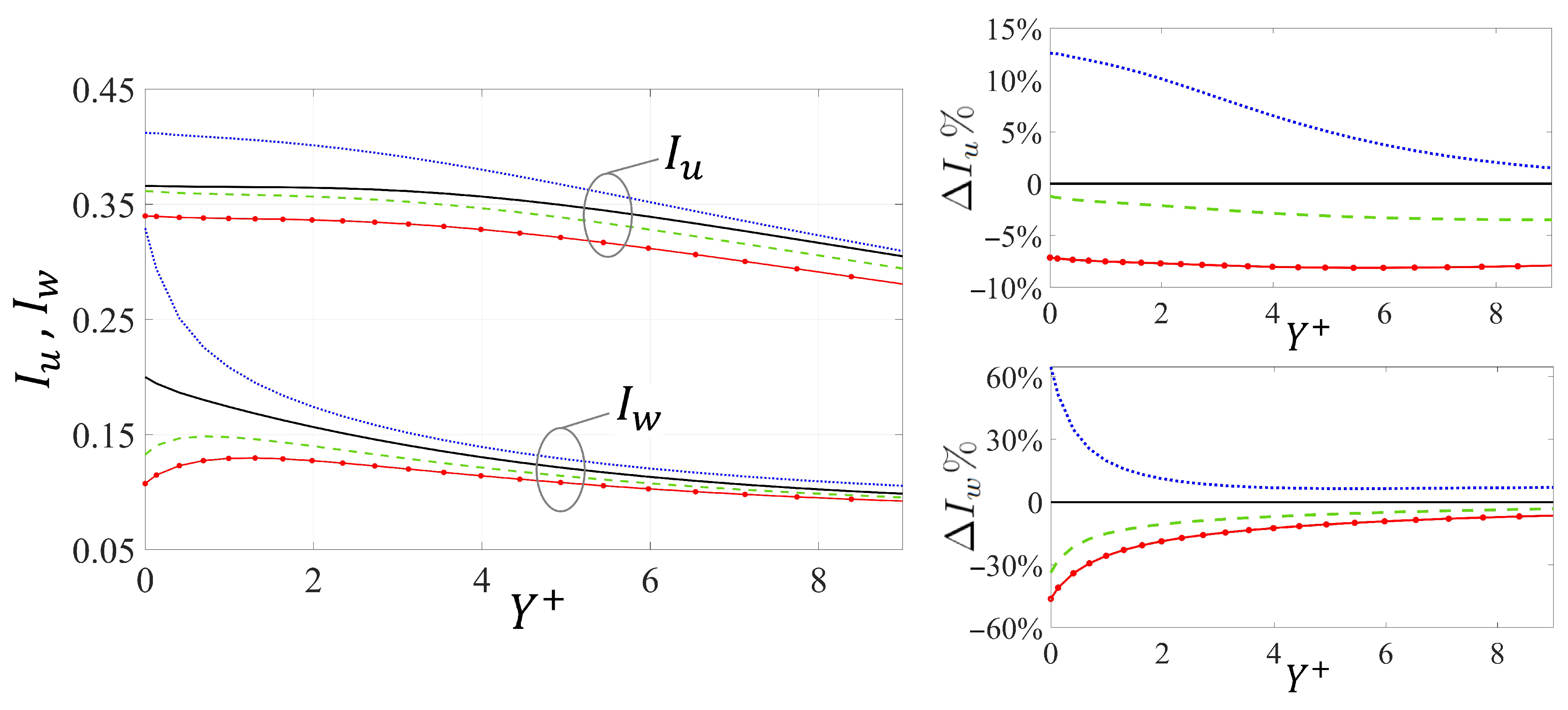
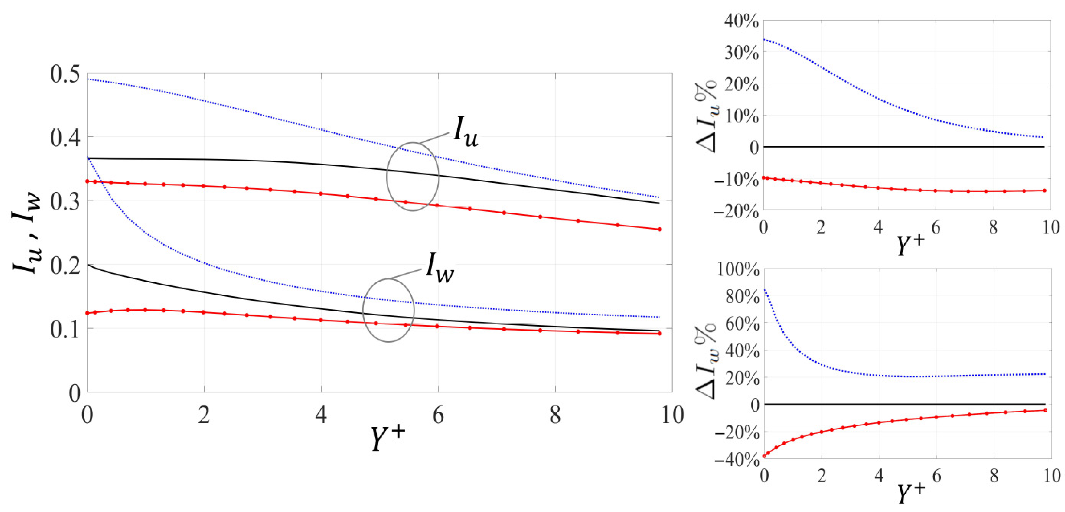
The analysis of the turbulence intensities and provides a meaningful picture of the levels of disturbances in the neighborhood of the permeable walls; such intensities can be used, together with the streamwise slip velocity, to interpret changes in skin-friction drag.
- (iv)
The implementation of the homogenization approach significantly reduces the numerical cost of direct numerical simulations over porous layers, since only the motion in the free-fluid region needs to be resolved. With the dimensions chosen for the domain, the total number of grid points is below
, while the mesh requirements for a full feature-resolving simulation (including the porous substrate) may exceed
(cf. Wang et al. [
24]).
The present approximate framework needs to be properly validated against feature-resolving simulations which include the permeable medium, in order to provide full confidence in the model developed. This task is currently underway and preliminary results are encouraging. Once this validation phase is terminated, the homogenization model developed will be employed in a large-scale optimization study: different microstructures of the porous substrate will be examined in pursuit of the
optimal topology, size and arrangement of the solid grains, capable to yield the largest skin-friction reduction. It will also be of interest to compare the homogenized results for porous substrates with inline and staggered arrangements of grains; this is the case since the configuration of randomly arranged inclusions might be expected to lie in between these two limiting cases, as observed by Naqvi and Bottaro [
42].


