Dynamic Equilibrium Equations in Unified Mechanics Theory

Abstract

Traditionally dynamic analysis is done using Newton’s universal laws of the equation of motion. According to the laws of Newtonian mechanics, the x, y, z, space-time coordinate system does not include a term for energy loss, an empirical damping term “C” is used in the dynamic equilibrium equation. Energy loss in any system is governed by the laws of thermodynamics. Unified Mechanics Theory (UMT) unifies the universal laws of motion of Newton and the laws of thermodynamics at ab-initio level. As a result, the energy loss [entropy generation] is automatically included in the laws of the Unified Mechanics Theory (UMT). Using unified mechanics theory, the dynamic equilibrium equation is derived and presented. One-dimensional free vibration analysis with frictional dissipation is used to compare the results of the proposed model with that of a Newtonian mechanics equation. For the proposed entropy generation equation in the system, the trend of predictions is comparable with the reported experimental results and Newtonian mechanics-based predictions.

1. Introduction

Many of mechanics’ problems involve the action of dissipative forces and hence the problem is to be dealt with the laws of thermodynamics [1] in addition to Newton’s laws of motion. In the context of thermodynamics, the work done by dissipative forces is known as pseudo-works [2]. These pseudo-works are treated as the equivalent heat dissipated, to explain the irreversibility of the process [3,4]. However, the heat dissipation is an outside quantity in Newton’s laws of motion. None of the real systems are conservative and hence, the dissipation process is essential to explain the irreversibility in mechanics. Since the mid-19th century, the unification of Newton’s laws of motion and laws of thermodynamics has been a pursuit of many researchers around the world. However, the fundamental procedure adopted in such attempts has been to incorporate suitable empirical energy dissipation parameters addressing problem-specific dissipation processes within the system [5]. Ludwig Boltzmann attempted to reduce thermodynamics to the time-reversible laws of Newton’s mechanics [6]. Boltzmann postulated that a transition from one configuration or microstate to another configuration or microstate is equally probable [7].

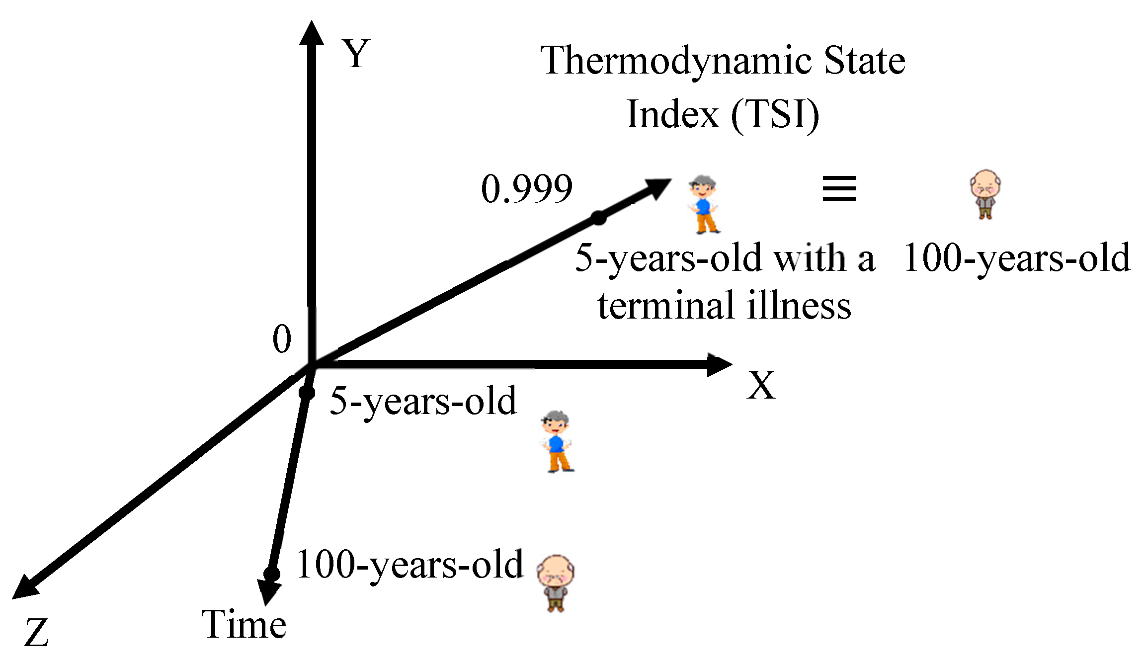
In the recent past, Boltzmann’s model for the irreversibility of dissipative processes has been unified with the laws of Newton [8], called unified mechanics theory [9]. In the unified mechanics’ theory (UMT) [9], dissipation mechanisms are represented by the Thermodynamics State Index (TSI) [9,10] of the system. The TSI represents the thermodynamic state of a physical system, as a function of entropy generation. Hence, the unified mechanics’ theory (UMT) explicitly introduces a new linearly independent axis in addition to Newtonian coordinates, x, y, z, and time [9,10].This concept was introduced [8,9,10,11] based on Boltzmann’s statistical relation of entropy with the probability of microstates within the system. Several published works can be seen in the literature, which address various types of dissipation processes, such as fatigue in metals [8,10,11,12], electromigration and thermomigration in nanoelectronics [13,14,15], damage in eutectic Pb/Sn solder joints [16,17,18], micromechanics of thermally induced dislocation annihilation [19], damage evolution in a particle-filled polymer matrix composite [20], damage due to concurrent thermal and vibration loading in electronic packaging [21], damage due to nanoindentation [22], etc. The TSI, $\mathsf{\Phi }$ represents an index called Thermodynamic State Index (TSI), as shown in Figure 1, which is a linearly independent axis, spanning between zero and one.

The coordinate system in the unified mechanics theory (UMT) is explained in the literature [9,10] as shown in Figure 1. Let us assume that there is a 5-year-old boy with a terminal illness and 100-year-old sick man. In Newtonian mechanics, both the 5-year-old boy and 100-year-old man, are represented by using Cartesian coordinates and time axis. Their physical states can only be represented by the laws of thermodynamics. However, in the unified mechanics, the thermodynamic state of both the 5-year-old boy with a terminal illness and 100-year-old sick man are represented by TSI axis, in addition to the space-time coordinates. On TSI axis at $\mathsf{\Phi }=0.999$, 5-year-old boy with a terminal illness and 100-year-old will have the same thermodynamic state index coordinate. TSI, $\mathsf{\Phi }$ is given by the following equation [8,9],

$$\mathsf{\Phi }={\mathsf{\Phi }}_{\mathrm{c}}\left[1-{\mathrm{e}}^{\left(-\Delta \mathrm{S}\frac{{\mathrm{m}}_{\mathrm{s}}}{\mathrm{R}}\right)}\right]$$

(1)

where, $\Delta \mathrm{S}$ represents total change in entropy calculated from the thermodynamic fundamental equation of the system, during the time, $\Delta \mathrm{t}$. The terms, ${\mathrm{m}}_{\mathrm{s}}$, ${\mathsf{\Phi }}_{\mathrm{c}}$, and $\mathrm{R}$ represent the molar mass, critical TSI value [10], and gas constant, respectively. If there are ‘n’ independent dissipation mechanisms in a system, general representation of the second law of unified mechanics theory [9], can be given as follows,

$${\displaystyle \sum }_{\mathrm{i}=1}^{\mathrm{n}}{\mathrm{F}}_{\mathrm{i}}\left({\mathsf{\Phi }}_{\mathrm{i}}\right)=\frac{\mathrm{d}\left(\mathrm{m}\left({\mathsf{\Phi }}_{\mathrm{m}}\right)\dot{\mathrm{u}}\right)}{\mathrm{dt}}$$

(2)

where, ${\mathrm{F}}_{\mathrm{i}}\left({\mathsf{\Phi }}_{\mathrm{i}}\right)$ is the ${\mathrm{i}}^{\mathrm{th}}$ force as a function of the thermodynamic state index which governs the dissipation in momentum, $\mathrm{m}\left({\mathsf{\Phi }}_{\mathrm{m}}\right)$ is the mass as a function of thermodynamic state index which governs the loss in mass. The concept given in Equation (2) denotes that, a physical system can undergo various independent dissipation processes along with the change in space-time coordinates of the system. Thermodynamics deals with dissipative mechanisms, representing the energy state of a system. Newton’s laws of motion give the space-time coordinates of a material point in a physical system. Thermodynamic fundamental equation of a system denotes the coordinate of the system on the TSI axis. Unified mechanics unifies Newton’s law of motion with the second law of thermodynamics, at an ab-initio level. In this study, our objective is to derive the dynamic equilibrium equation of a dissipative system and compare the results of the unified mechanics theory (UMT) with that of a Newtonian mechanics equation of motion. A free vibration analysis on a mass-spring single degree of freedom system subjected to sliding friction is done to demonstrate the results in both cases. Sliding friction is a dissipative process. In Newton’s model, the sliding friction is accounted for by frictional force. Coulombs model for friction is dependent on the applied normal contact force and independent of the area of contact and velocity of motion. In Newton’s equation of motion for dynamic equilibrium, the Coulomb model for friction uses an experimental curve-fitted parameter called a frictional coefficient to account for the non-conservative generalized force due to frictional dissipation. Variants of Coulomb’s model for dynamic analysis are reported in the literature [23]. Even though Newton’s laws of motion do not directly account for the thermodynamics of frictional dissipation, the Coulomb model for frictional dissipation is empirically incorporated in Newtonian mechanics models [24,25,26,27,28] by adding a frictional damping term “C” in the equation of motion. Since 1895, when Painlevé first discovered the incompatibility of frictional dissipation with Newtonian mechanics [29], many researchers have been attempting to resolve the paradox [30,31]. In tribology, frictional dissipation has been introduced with the concept of thermodynamic quantity, known as entropy [32,33]. Such a thermodynamic approach of introducing friction using entropy is often questioned for its practical feasibility [32]. Unified mechanics theory deals with the mechanics of both the conservative and non-conservative systems. In this study we present a novel and practically feasible approach to introduce friction as a thermodynamic dissipative process, and solve one-dimensional free vibration problems, using the unified mechanics’ theory. The presented approach is thermodynamically consistent and requires no empirical addition of functionals or curve-fit methods to introduce dissipative terms in the dynamic equilibrium equation.

The work is organized as follows. In Section 2, a basic form of dynamic equilibrium equation is derived from the general form Lagrangian and using fundamental principles of finding the local extremum of integrals. A mass-spring single degree of freedom system subjected to sliding contact friction is considered to derive a dynamic equilibrium equation for the specific case, using the equation derived in Section 2, and the derivation is presented in Section 3. An entropy generation function under sliding contact friction is presented in Section 4. Using the dynamic equilibrium equation derived in Section 3 and the thermodynamics fundamental equation of the system presented in Section 4, free vibration analysis is done and the results are presented along with the results using the Newtonian mechanics’ equilibrium equation and test data, in Section 5. The main conclusions from the observations on the proposed model and the results are presented in Section 6.

2. Derivation of the Dynamic Equilibrium Equation

The action of a material point, over a period,$\Delta \mathrm{t}={\mathrm{t}}_2-{\mathrm{t}}_1$, can be defined by the following integral,

$$\mathrm{I}={{\displaystyle \int }}_{{\mathrm{t}}_1}^{{\mathrm{t}}_2}\mathcal{L} \mathrm{dt}$$

(3)

where $\mathcal{L}$ represents the Lagrangian of the system [34]. Classical mechanics using Lagrangian applies to macroscopic systems under energy-conserving motion. If irreversible processes are to be included in the Lagrangian, the second law of thermodynamics must be considered [3]. In Newtonian mechanics, the effect of dissipative forces is included as impulsive forces and pseudo-forces [4]. Hence, the Newtonian mechanics deals with space-time coordinates and does not consider a change in entropy of the system. In recent years, some research works are focusing on the formulation of dissipative processes in Lagrangian formalism. For example, Musielak [35] introduced first-order time derivative terms (functions in terms of velocity) with coefficients varying in time or space, to include the dissipative terms in the Lagrangian of dynamical systems. Lazo and Kumreich [36] proposed Lagrangian function, depending on mixed-integer order and fractional order derivatives to formulate a quadratic Lagrangian for non-conservative systems. Even though the approach [36] is consistent with the variational principles, the Riemann-Liouville fractional derivatives in the Lagrangian, were introduced without any thermodynamic basis. Mart´ınez-P´erez and Ram´ırez [37] studied the doubled variable Lagrangian formulation of dissipative mechanical systems by the application of the Noether theorem. Szegleti and Márkus [38] presented a method which creates a potential function that generates the measurable physical quantity, to describe a dissipative system modeled by a linear differential equation in Lagrangian formalism. It is stated in the literature [38] that the numerical solutions to the differential equations formulated by the presented [38] method would yield non-physical solutions, if not stabilized by appropriate conditions. However, the method [38] did not give any physical basis in incorporating a potential in the Lagrangian. None of the above approaches brought the idea to describe dissipation within Lagrangian formalism based on the second law of thermodynamics.

In this study, we attempt to introduce second law of thermodynamics in the Lagrangian system, using the unified mechanics theory. In the unified mechanics theory [8,9,10], each material point in a dynamics problem is defined in the space-time-TSI coordinate system. Hence the material point shall be a function of $\left(\mathrm{x},\mathrm{t},\mathsf{\Phi }\right)$. The additional parameter $\mathsf{\Phi }$, called Thermodynamic State Index (TSI) [9,10] of the material point represents the physical state (corresponding to an entropy generation mechanism) of the material point. Using the unified mechanics theory [9], Lagrangian of the system is written as follows,

$$\mathcal{L}=\mathcal{L}\left(\mathrm{t},\mathrm{u},\dot{\mathrm{u}},{\mathsf{\Phi }}_{\mathrm{i}}\right)$$

(4)

where $\mathrm{u}$ and $\dot{\mathrm{u}}$ represents displacement and velocity of a material point, respectively. The term ${\mathsf{\Phi }}_{\mathrm{i}}$ is used represent n number of different independent dissipation mechanisms within a given thermodynamic system at a material point. If the integral function in Equation (3) attains a local minimum at a point, $\mathrm{q}$ and let $\mathsf{\zeta }\left(\mathrm{t}\right)$ be an arbitrary function that has at least one derivative and vanishes at the initial time, ${\mathrm{t}}_1$ and final time,${ \mathrm{t}}_2$; then for any real number $\mathsf{ϵ}$, closer to zero, the following condition is valid,

$$\mathrm{I}\left(\mathrm{q}\right)\le \mathrm{J}\left(\mathsf{ϵ}\right)$$

(5)

where the real-valued function, $\mathrm{J}$ is represented as follows,

$$\mathrm{J}\left(\mathsf{ϵ}\right)=\mathrm{I}\left(\mathrm{q}+\mathsf{ϵ}\mathsf{\zeta }\right)$$

(6)

The functional ‘$\mathrm{I}$’ is said to have a local minimum at $\mathrm{u}=\mathrm{q}$, the function $\mathrm{J}$ equivalently has a local minimum at $\mathsf{ϵ}=0$. Hence the following equation is valid,

$${\left[\frac{\mathrm{dJ}}{\mathrm{d}\mathsf{ϵ}}\right]}_{\mathsf{ϵ}=0}={{\displaystyle \int }}_{{\mathrm{t}}_1}^{{\mathrm{t}}_2}{\left[\frac{\mathrm{d}\mathcal{L}}{\mathrm{d}\mathsf{ϵ}}\right]}_{\mathsf{ϵ}=0}\mathrm{dt}=0$$

(7)

Taking the total derivative of $\mathcal{L}$, we get the following equation, which has an additional term compared to Newtonian mechanics,

$$\frac{\mathrm{d}\mathcal{L}}{\mathrm{d}\mathsf{ϵ}}=\frac{\partial \mathcal{L}}{\partial \mathrm{u}}\frac{\mathrm{du}}{\mathrm{d}\mathsf{ϵ}}+\frac{\partial \mathcal{L}}{\partial \dot{\mathrm{u}}}\frac{\mathrm{d} \dot{\mathrm{u}}}{\mathrm{d}\mathsf{ϵ}}+{\displaystyle \sum }_{\mathrm{i}=1}^{\mathrm{n}}\frac{\partial \mathcal{L}}{\partial {\mathsf{\Phi }}_{\mathrm{i}}}\frac{{\mathrm{d}\mathsf{\Phi }}_{\mathrm{i}}}{\mathrm{d}\mathsf{ϵ}}$$

(8)

It is important to note in Equation (8) that the derivative of Lagrangian with respect to the new axis, TSI is non-zero. The displacement is represented as follows,

$$\mathrm{u}=\mathrm{q}+\mathsf{ϵ}\mathsf{\zeta }$$

(9)

Taking the time derivative of Equation (9), we get the following equation for velocity,

$$\dot{\mathrm{u}}=\dot{\mathrm{q}}+\mathsf{ϵ}\dot{\mathsf{\zeta }}$$

(10)

Using Equations (9) and (10), we get the following form for Equation (8),

$$\frac{\mathrm{d}\mathcal{L}}{\mathrm{d}\mathsf{ϵ}}=\frac{\partial \mathcal{L}}{\partial \mathrm{u}}\mathsf{\zeta }+\frac{\partial \mathcal{L}}{\partial \dot{\mathrm{u}}}\dot{\mathsf{\zeta }}+{\displaystyle \sum }_{\mathrm{i}=1}^{\mathrm{n}}\frac{\partial \mathcal{L}}{\partial {\mathsf{\Phi }}_{\mathrm{i}}}\frac{{\mathrm{d}\mathsf{\Phi }}_{\mathrm{i}}}{\mathrm{d}\mathsf{ϵ}}$$

(11)

In this study, we consider a friction driven dissipation mechanism for a single degree of freedom mass-spring system, subjected to Coulomb friction. Hence, with the TSI, ${\mathsf{\Phi }}_{\mathrm{i}}=\mathsf{\Phi }\left(\mathrm{u},\dot{\mathrm{u}},\mathrm{t}\right)$ and we write the following total derivative of $\mathsf{\Phi }$ with respect to $\mathsf{ϵ}$,

$$\frac{\mathrm{d}\mathsf{\Phi }}{\mathrm{d}\mathsf{ϵ}}=\frac{\partial \mathsf{\Phi }}{\partial \mathrm{u}}\frac{\mathrm{du}}{\mathrm{d}\mathsf{ϵ}}+\frac{\partial \mathsf{\Phi }}{\partial \dot{\mathrm{u}}}\frac{\mathrm{d}\dot{\mathrm{u}}}{\mathrm{d}\mathsf{ϵ}}$$

(12)

Hence, by substituting Equation (12) in Equation (11), we get the following equation,

$$\frac{\mathrm{d}\mathcal{L}}{\mathrm{d}\mathsf{ϵ}}=\left(\frac{\partial \mathcal{L}}{\partial \mathrm{u}}+\frac{\partial \mathcal{L}}{\partial \mathsf{\Phi }}\frac{\partial \mathsf{\Phi }}{\partial \mathrm{u}}\right)\mathsf{\zeta }+\left(\frac{\partial \mathcal{L}}{\partial \dot{\mathrm{u}}}+\frac{\partial \mathcal{L}}{\partial \mathsf{\Phi }}\frac{\partial \mathsf{\Phi }}{\partial \dot{\mathrm{u}}}\right)\dot{\mathsf{\zeta }}$$

(13)

Therefore, Equation (7) takes the following form,

$${{\displaystyle \int }}_{{\mathrm{t}}_1}^{{\mathrm{t}}_2}{\left[\frac{\mathrm{d}\mathcal{L}}{\mathrm{d}\mathsf{ϵ}}\right]}_{\mathsf{ϵ}=0} \mathrm{dt}={{\displaystyle \int }}_{{\mathrm{t}}_1}^{{\mathrm{t}}_2}{\left[\left(\frac{\partial \mathcal{L}}{\partial \mathrm{u}}+\frac{\partial \mathcal{L}}{\partial \mathsf{\Phi }}\frac{\partial \mathsf{\Phi }}{\partial \mathrm{u}}\right)\mathsf{\zeta }\right]}_{\mathsf{ϵ}=0}\mathrm{dt}+{{\displaystyle \int }}_{{\mathrm{t}}_1}^{{\mathrm{t}}_2}{\left[\left(\frac{\partial \mathcal{L}}{\partial \dot{\mathrm{u}}}+\frac{\partial \mathcal{L}}{\partial \mathsf{\Phi }}\frac{\partial \mathsf{\Phi }}{\partial \dot{\mathrm{u}}}\right)\dot{\mathsf{\zeta }}\right]}_{\mathsf{ϵ}=0}\mathrm{dt}=0$$

(14)

Integrating the second term on the right-hand side of Equation (14) by parts, we get the following equation,

$${{\displaystyle \int }}_{{\mathrm{t}}_1}^{{\mathrm{t}}_2}{\left[\left(\frac{\partial \mathcal{L}}{\partial \mathrm{u}}+\frac{\partial \mathcal{L}}{\partial \mathsf{\Phi }}\frac{\partial \mathsf{\Phi }}{\partial \mathrm{u}}-\frac{\mathrm{d}}{\mathrm{dt}}\left(\frac{\partial \mathcal{L}}{\partial \dot{\mathrm{u}}}+\frac{\partial \mathcal{L}}{\partial \mathsf{\Phi }}\frac{\partial \mathsf{\Phi }}{\partial \dot{\mathrm{u}}}\right)\right)\mathsf{\zeta }\right]}_{\mathsf{ϵ}=0}\mathrm{dt}+{\left\{\left(\frac{\partial \mathcal{L}}{\partial \dot{\mathrm{u}}}+\frac{\partial \mathcal{L}}{\partial \mathsf{\Phi }}\frac{\partial \mathsf{\Phi }}{\partial \dot{\mathrm{u}}}\right){\left[\mathsf{\zeta }\right]}_{\mathsf{ϵ}=0}\right\}}_{{\mathrm{t}}_1}^{{\mathrm{t}}_2}=0$$

(15)

By the definition of $\mathsf{\zeta }$, the second term in Equation (15) vanishes at the boundary of the integral domain. Hence, using Equations (9) and (10) in Equation (14) and by applying the principle of local state, we get the following equation,

$$\frac{\partial \mathcal{L}}{\partial \mathrm{u}}+\frac{\partial \mathcal{L}}{\partial \mathsf{\Phi }}\frac{\partial \mathsf{\Phi }}{\partial \mathrm{u}}-\frac{\mathrm{d}}{\mathrm{dt}}\left(\frac{\partial \mathcal{L}}{\partial \dot{\mathrm{u}}}+\frac{\partial \mathcal{L}}{\partial \mathsf{\Phi }}\frac{\partial \mathsf{\Phi }}{\partial \dot{\mathrm{u}}}\right)=0$$

(16)

Unlike in the Newtonian mechanics-based Euler-Lagrange equation, Equation (16) has an additional derivative as a function of TSI. Using Equation (9), the variation statement of any function, $\mathsf{\Psi }$ in $\mathrm{u}$, is represented as follows.

$${\left[\frac{\mathrm{d}\mathsf{\Psi }}{\mathrm{d}\mathsf{ϵ}}\right]}_{\mathsf{ϵ}=0}=\mathsf{\delta }\mathsf{\Psi }$$

(17)

Using Lagrange-d’Alembert’s principle, and representation of variation statement, given in Equation (17), for an externally applied force,${ \mathrm{F}}_{\mathrm{ext}}$, we can write the following equation,

$$\frac{\partial \mathcal{L}}{\partial \mathrm{u}}+\frac{\partial \mathcal{L}}{\partial \mathsf{\Phi }}\frac{\partial \mathsf{\Phi }}{\partial \mathrm{u}}-\frac{\mathrm{d}}{\mathrm{dt}}\left(\frac{\partial \mathcal{L}}{\partial \dot{\mathrm{u}}}+\frac{\partial \mathcal{L}}{\partial \mathsf{\Phi }}\frac{\partial \mathsf{\Phi }}{\partial \dot{\mathrm{u}}}\right)+{\mathrm{F}}_{\mathrm{ext}}=0$$

(18)

Equation (18) represents the basic form of dynamic equilibrium equation in unified mechanics theory. Specific form for a given system is derived by writing the fundamental equation for entropy generation in the system and the Lagrangian of the system. In the succeeding section, a mass-spring system with friction as the source of dissipation is considered to apply the basic form of structural dynamic equilibrium equation given in Equation (18).

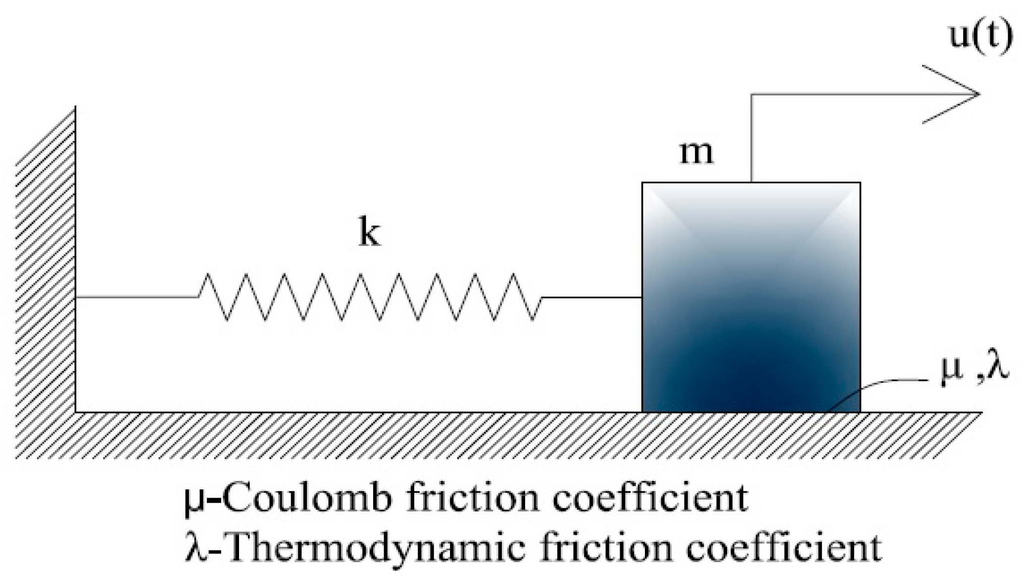
3. Application of the Equation on the Vibration of a Mass-spring System Subjected to Friction

In this section, a mass-spring system under frictional dissipation is used to derive the governing equation of motion using Equation (18) and compare the solution of the equation of motion with that of a Newtonian mechanics equilibrium equation. A schematic representation of the mass-spring system is given in Figure 2.

Lagrangian of the system is given by,

$$\mathcal{L}=\mathrm{K}-\mathrm{V}$$

(19)

where $\mathrm{K}$ and $\mathrm{V}$ are the total kinetic energy and total potential energy of the system, respectively. In the derivation, mass is considered to be constant and hence, ${\mathsf{\Phi }}_{\mathrm{m}}=0$, in Equation (2). For a mass $\mathrm{m}$, excited by an external force, ${\mathrm{F}}_{\mathrm{ext}}\left(\mathrm{t}\right)$, the total kinetic energy of a conservative system (without damping) is given by the following equation,

$$\mathrm{K}=\frac{1}{2}\mathrm{m}{\dot{\tilde{\mathrm{u}}}}^2$$

(20)

where, the velocity, $\dot{\tilde{\mathrm{u}}}$ in Equation (20), represents the velocity of a mass-spring system in Newtonian mechanics with no dissipation due to friction. Using unified mechanics theory, any dissipative processes in a system can be modeled by using TSI, $\mathsf{\Phi }$. TSI, $\mathsf{\Phi }$ is an index, which evolves from zero to one, as a function of entropy generation. Hence, we represent the net kinetic energy of the mass m, with a resultant velocity, $\dot{\mathrm{u}}$ as follows,

$$\frac{1}{2}{\mathrm{m}\dot{\mathrm{u}}}^2=\frac{1}{2}\mathrm{m}{\dot{\tilde{\mathrm{u}}}}^2\left(1-\mathsf{\Phi }\right)$$

(21)

the potential energy is expressed similarly, by introducing entropy generation due to friction. Hence, the Lagrangian in the unified mechanics theory is given by the following equation,

$$\mathcal{L}=\frac{1}{2}\mathrm{m}{\dot{\tilde{\mathrm{u}}}}^2-\frac{1}{2}{\mathrm{k}\tilde{\mathrm{u}}}^2=\frac{1}{\left(1-\mathsf{\Phi }\right)}\frac{1}{2}{\mathrm{m}\dot{\mathrm{u}}}^2-\frac{1}{\left(1-\mathsf{\Phi }\right)}\frac{1}{2}{\mathrm{ku}}^2$$

(22)

In Equation (22), entropy generation due to degradation in spring stiffness is ignored.

Derivative terms in Equation (18) are calculated using Equation (22) as follows,

$$\frac{\partial \mathcal{L}}{\partial \mathrm{u}}=-{\left(1-\mathsf{\Phi }\right)}^{-1}\mathrm{ku}$$

(23)

$$\frac{\partial \mathcal{L}}{\partial \mathsf{\Phi }}=\frac{1}{{\left(1-\mathsf{\Phi }\right)}^2}\frac{1}{2}{\mathrm{m}\dot{\mathrm{u}}}^2-\frac{1}{{\left(1-\mathsf{\Phi }\right)}^2}\frac{1}{2}{\mathrm{ku}}^2$$

(24)

$$\frac{\partial \mathsf{\Phi }}{\partial \mathrm{u}}=\frac{{\mathrm{m}}_{\mathrm{s}}}{\mathrm{R}}{\mathrm{e}}^{\left(-\Delta \mathrm{S}\frac{{\mathrm{m}}_{\mathrm{s}}}{\mathrm{R}}\right)}\frac{\partial \Delta \mathrm{S}}{\partial \mathrm{u}}=\frac{{\mathrm{m}}_{\mathrm{s}}}{\mathrm{R}}\left(1-\mathsf{\Phi }\right)\frac{\partial \Delta \mathrm{S}}{\partial \mathrm{u}}$$

(25)

$$\frac{\partial \mathcal{L}}{\partial \dot{\mathrm{u}}}={\left(1-\mathsf{\Phi }\right)}^{-1}\mathrm{m}\dot{\mathrm{u}}$$

(26)

$$\begin{gathered} \frac{\mathrm{d}}{\mathrm{dt}}\left(\frac{\partial \mathcal{L}}{\partial \dot{\mathrm{u}}}\right)=\mathrm{m}\dot{\mathrm{u}}\frac{\mathrm{d}}{\mathrm{dt}}\left({\left(1-\mathsf{\Phi }\right)}^{-1}\right)+\frac{1}{\left(1-\mathsf{\Phi }\right)}\mathrm{m}\ddot{\mathrm{u}} \\ \mathrm{or}, \\ \frac{\mathrm{d}}{\mathrm{dt}}\left(\frac{\partial \mathcal{L}}{\partial \dot{\mathrm{u}}}\right)=\mathrm{m}\dot{\mathrm{u}}\frac{\left(\frac{\mathrm{d}\mathsf{\Phi }}{\mathrm{dt}}\right)}{{\left(1-\mathsf{\Phi }\right)}^2}+\frac{1}{\left(1-\mathsf{\Phi }\right)}\mathrm{m}\ddot{\mathrm{u}} \end{gathered}$$

(27)

$$\frac{\mathrm{d}\mathsf{\Phi }}{\mathrm{dt}}=\frac{{\mathrm{m}}_{\mathrm{s}}}{\mathrm{R}}\left(1-\mathsf{\Phi }\right)\frac{\mathrm{d}\Delta \mathrm{S}}{\mathrm{dt}}$$

(28)

$$\frac{\mathrm{d}}{\mathrm{dt}}\left(\frac{\partial \mathcal{L}}{\partial \mathsf{\Phi }}\frac{\partial \mathsf{\Phi }}{\partial \dot{\mathrm{u}}}\right)=\frac{\mathrm{d}}{\mathrm{dt}}\left(\frac{\partial \mathcal{L}}{\partial \mathsf{\Phi }}\right)\frac{\partial \mathsf{\Phi }}{\partial \dot{\mathrm{u}}}+\frac{\partial \mathcal{L}}{\partial \mathsf{\Phi }}\frac{\mathrm{d}}{\mathrm{dt}}\left(\frac{\partial \mathsf{\Phi }}{\partial \dot{\mathrm{u}}}\right)$$

(29)

$$\begin{gathered} \frac{\mathrm{d}}{\mathrm{dt}}\left(\frac{\partial \mathcal{L}}{\partial \mathsf{\Phi }}\right)=\frac{\mathrm{d}}{\mathrm{dt}}\left(\frac{1}{{\left(1-\mathsf{\Phi }\right)}^2}\frac{1}{2}{\mathrm{m}\dot{\mathrm{u}}}^2\right)-\frac{\mathrm{d}}{\mathrm{dt}}\left(\frac{1}{{\left(1-\mathsf{\Phi }\right)}^2}\frac{1}{2}{\mathrm{ku}}^2\right) \\ =\frac{1}{2}{\mathrm{m}\dot{\mathrm{u}}}^2\frac{\mathrm{d}}{\mathrm{dt}}\left(\frac{1}{{\left(1-\mathsf{\Phi }\right)}^2}\right)+\frac{1}{{\left(1-\mathsf{\Phi }\right)}^2}\frac{\mathrm{d}}{\mathrm{dt}}\left(\frac{1}{2}{\mathrm{m}\dot{\mathrm{u}}}^2\right)-\frac{1}{2}{\mathrm{ku}}^2\frac{\mathrm{d}}{\mathrm{dt}}\left(\frac{1}{{\left(1-\mathsf{\Phi }\right)}^2}\right)-\frac{1}{{\left(1-\mathsf{\Phi }\right)}^2}\frac{\mathrm{d}}{\mathrm{dt}}\left(\frac{1}{2}{\mathrm{ku}}^2\right) \\ \mathrm{or}, \\ \frac{\mathrm{d}}{\mathrm{dt}}\left(\frac{\partial \mathcal{L}}{\partial \mathsf{\Phi }}\right)=\left(\frac{1}{2}{\mathrm{m}\dot{\mathrm{u}}}^2-\frac{1}{2}{\mathrm{ku}}^2\right)\left(\frac{1}{{\left(1-\mathsf{\Phi }\right)}^2}2\frac{{\mathrm{m}}_{\mathrm{s}}}{\mathrm{R}}\frac{\mathrm{d}\Delta \mathrm{S}}{\mathrm{dt}}\right)+\frac{1}{{\left(1-\mathsf{\Phi }\right)}^2}\left(\mathrm{m}\ddot{\mathrm{u}}-\mathrm{ku}\right)\dot{\mathrm{u}} \end{gathered}$$

(30)

$$\frac{\partial \mathsf{\Phi }}{\partial \dot{\mathrm{u}}}=\frac{{\mathrm{m}}_{\mathrm{s}}}{\mathrm{R}}\left(1-\mathsf{\Phi }\right)\frac{\partial \Delta \mathrm{S}}{\partial \dot{\mathrm{u}}}$$

(31)

$$\begin{gathered} \frac{\mathrm{d}}{\mathrm{dt}}\left(\frac{\partial \mathsf{\Phi }}{\partial \dot{\mathrm{u}}}\right)=\frac{{\mathrm{m}}_{\mathrm{s}}}{\mathrm{R}}\frac{\mathrm{d}}{\mathrm{dt}}\left(\left(1-\mathsf{\Phi }\right)\frac{\partial \Delta \mathrm{S}}{\partial \dot{\mathrm{u}}}\right) \\ =\frac{{\mathrm{m}}_{\mathrm{s}}}{\mathrm{R}}\frac{\partial \Delta \mathrm{S}}{\partial \dot{\mathrm{u}}}\frac{\mathrm{d}}{\mathrm{dt}}\left(\left(1-\mathsf{\Phi }\right)\right)+\frac{{\mathrm{m}}_{\mathrm{s}}}{\mathrm{R}}\left(1-\mathsf{\Phi }\right)\frac{\mathrm{d}}{\mathrm{dt}}\left(\frac{\partial \Delta \mathrm{S}}{\partial \dot{\mathrm{u}}}\right) \\ \mathrm{or}, \\ \frac{\mathrm{d}}{\mathrm{dt}}\left(\frac{\partial \mathsf{\Phi }}{\partial \dot{\mathrm{u}}}\right)=\frac{{\mathrm{m}}_{\mathrm{s}}}{\mathrm{R}}\left(1-\mathsf{\Phi }\right)\frac{\mathrm{d}}{\mathrm{dt}}\left(\frac{\partial \Delta \mathrm{S}}{\partial \dot{\mathrm{u}}}\right)-{\left(\frac{{\mathrm{m}}_{\mathrm{s}}}{\mathrm{R}}\right)}^2\left(1-\mathsf{\Phi }\right)\frac{\partial \Delta \mathrm{S}}{\partial \dot{\mathrm{u}}}\frac{\mathrm{d}\Delta \mathrm{S}}{\mathrm{dt}} \end{gathered}$$

(32)

$$\begin{gathered} \frac{\mathrm{d}}{\mathrm{dt}}\left(\frac{\partial \mathcal{L}}{\partial \mathsf{\Phi }}\frac{\partial \mathsf{\Phi }}{\partial \dot{\mathrm{u}}}\right)=\left\{\left(\frac{1}{2}{\mathrm{m}\dot{\mathrm{u}}}^2-\frac{1}{2}{\mathrm{ku}}^2\right)\left(\frac{1}{{\left(1-\mathsf{\Phi }\right)}^2}2\frac{{\mathrm{m}}_{\mathrm{s}}}{R}\frac{\mathrm{d}\Delta \mathrm{S}}{\mathrm{dt}}\right) \\ +\frac{1}{{\left(1-\mathsf{\Phi }\right)}^2}\left(\mathrm{m}\ddot{\mathrm{u}}-\mathrm{ku}\right)\dot{\mathrm{u}}\right\}\frac{{\mathrm{m}}_{\mathrm{s}}}{\mathrm{R}}\left(1-\mathsf{\Phi }\right)\frac{\partial \Delta \mathrm{S}}{\partial \dot{\mathrm{u}}} \\ +\left\{\frac{1}{{\left(1-\mathsf{\Phi }\right)}^2}\frac{1}{2}{\mathrm{m}\dot{\mathrm{u}}}^2-\frac{1}{{\left(1-\mathsf{\Phi }\right)}^2}\frac{1}{2}{\mathrm{ku}}^2\right\}\left\{\frac{{\mathrm{m}}_{\mathrm{s}}}{\mathrm{R}}\left(1-\mathsf{\Phi }\right)\frac{\mathrm{d}}{\mathrm{dt}}\left(\frac{\partial \Delta \mathrm{S}}{\partial \dot{\mathrm{u}}}\right) \\ -{\left(\frac{{\mathrm{m}}_{\mathrm{s}}}{\mathrm{R}}\right)}^2\left(1-\mathsf{\Phi }\right)\frac{\partial \Delta \mathrm{S}}{\partial \dot{\mathrm{u}}}\frac{\Delta \mathrm{S}}{\mathrm{dt}}\right\} \end{gathered}$$

(33)

Using Equation (1), Equation (18), and Equation (23) through Equation (33), we get the following force balance equilibrium equation,

$$\frac{1}{\left(1-\mathsf{\Phi }\right)}\mathrm{m}\ddot{\mathrm{u}}+\frac{1}{\left(1-\mathsf{\Phi }\right)}\mathrm{ku}+\left(\mathrm{m}\frac{{\mathrm{m}}_{\mathrm{s}}}{\mathrm{R}}\frac{1}{\left(1-\mathsf{\Phi }\right)}\frac{\mathrm{d}\Delta \mathrm{S}}{\mathrm{dt}}\right)\dot{\mathrm{u}}+\frac{{\mathrm{m}}_{\mathrm{s}}}{\mathrm{R}}\frac{1}{\left(1-\mathsf{\Phi }\right)}\left\{\frac{1}{2}{\mathrm{ku}}^2-\frac{1}{2}{\mathrm{m}\dot{\mathrm{u}}}^2\right\}\frac{\partial \Delta \mathrm{S}}{\partial \mathrm{u}}+ℊ\left(\frac{\partial \Delta \mathrm{S}}{\partial \dot{\mathrm{u}}}\right)+{\mathrm{F}}_{\mathrm{ext}}=0$$

(34)

The function, $ℊ$ is the summation of all the terms as a function of $\frac{\partial \Delta \mathrm{S}}{\partial \dot{\mathrm{u}}}$ and ${\mathrm{F}}_{\mathrm{ext}}$ is the external excitation force.

On the other hand, in Newtonian mechanics, the governing equation of motion under sliding friction is given by the following equation,

$$\mathrm{m}\ddot{\mathrm{u}}+\mathrm{ku}+\mathsf{\mu }\mathrm{mg} \mathrm{sgn}\left(\dot{\mathrm{u}}\right)+{\mathrm{F}}_{\mathrm{ext}}=0$$

(35)

where, μ is the Coulomb friction coefficient, m is the mass, g is the gravitational constant, and $\mathrm{sgn}$ is the signum function. The damping term ‘C’ in Equation (35) is represented by the Coulomb friction force. Equation (35) does not include any dissipation other than mechanical work due to friction. However, there are also other dissipative processes that are accounted for in unified mechanics equilibrium Equation (34). These additional entropy generation mechanisms are defined in terms of change in entropy, $\Delta \mathrm{S},$ and energy loss, represented along the thermodynamic state index axis, $\mathsf{\Phi }$. The entropy generation function during the sliding friction is derived in the following section.

4. Entropy Generation in Sliding Friction Contact: Thermodynamic Fundamental Equation

Sliding friction is a dissipative mechanism. Experimental results on free vibration of a single degree of freedom system with Coulomb friction shows that the decay in the amplitude of free vibration is bilinear and linearity is lost towards the end of vibration [39,40,41]. However, such bi-linearity is not captured in the Newtonian mechanics’ equation given in Equation (35). There are several dissipation mechanisms in sliding friction, such as mechanical work dissipation, heat generation [33], and acoustic losses [42]. In this section, we attempt to derive an entropy generation equation for the sliding friction in a single degree of freedom mass-spring system. Mechanical work dissipated during friction sliding is given by the following equation,

$${\mathrm{W}}_{\mathrm{m}}={{\displaystyle \int }}_{{\mathrm{t}}_1}^{{\mathrm{t}}_2}\mathsf{\mu }\mathrm{mg}\left|\mathrm{du}\right|$$

(36)

The coefficient of friction is obtained empirically. It is defined by the critical force that causes the onset of sliding. But it does not account for heating caused by sliding, and acoustic losses. The heat generation during sliding friction is dependent on the velocity of motion [33]. Temperature rise due to heating of the contact surfaces increases the entropy generation. A very large increment in temperature leads to diffusion of the material and such process is applied in friction welding applications [43]. This study does not deal with such diffusion mechanisms due to heating. Since the current study is limited to the derivation of the dynamic equilibrium equation of unified mechanics theory for a dynamic event and to demonstrating the application of the resulting governing equation of motion, this study does not deal with the derivation of the fundamental equation for diffusion in sliding friction. Nevertheless, for the validation of the proposed governing equation of motion, we propose a model for dissipation due to the probable mechanisms other than mechanical dissipation given in Equation (36). It is postulated that the dissipation due to all other mechanisms, such as heating and acoustics, is directly proportional to dissipation due to mechanical sliding, given in Equation (36). Hence, we give the following relation to total dissipation,

$${\mathrm{W}}_{\mathrm{d}}^{\mathrm{T}}=\left(1+{\mathsf{\kappa }}_{\mathrm{d}}\right){\mathrm{W}}_{\mathrm{m}}$$

(37)

where,${ \mathrm{W}}_{\mathrm{d}}^{\mathrm{T}}$ is the total dissipation and ${\mathsf{\kappa }}_{\mathrm{d}}$ is the fraction of work dissipated as heat, acoustic losses, etc. Since the proposed model is based on the second law of thermodynamics for dissipation mechanism, entropy generation, $\Delta \mathrm{S}$, representing the dissipation process in a mass-spring system under friction has to be calibrated with an in-efficiency parameter. The initial potential energy of the mass-spring system under free-vibration will be dissipated as work of friction, heat, and acoustic losses. However, this conversion cannot be perfect. Hence, the specific entropy generated is given by the following equation,

$$\Delta \mathrm{S}=\frac{1}{\mathrm{mT}}\left(1+{\mathsf{\kappa }}_{\mathrm{d}}\right){\mathsf{\psi }}_{\mathrm{s}}{{\displaystyle \int }}_{{\mathrm{t}}_1}^{{\mathrm{t}}_2}\mathrm{m}\mathsf{\mu }\mathrm{g}\left|\mathrm{du}\right|$$

(38)

where ${\mathsf{\psi }}_{\mathrm{s}}$ represents the in-efficiency factor. We define the factor, ${\mathsf{\psi }}_{\mathrm{s}}$ as the ratio between the maximum entropy at which TSI, $\mathsf{\Phi }$ tends to unity (say, at $\mathsf{\Phi }=0.99$) and the maximum entropy that the mass-spring system could generate, for an initial excitation, if it had zero in-efficiency. Hence, by substituting Equation (38) in Equation (34), we get the following equation,

$$\frac{1}{\left(1-\mathsf{\Phi }\right)}\mathrm{m}\ddot{\mathrm{u}}+\frac{1}{\left(1-\mathsf{\Phi }\right)}\mathrm{ku}+\frac{{\mathrm{m}}_{\mathrm{s}}}{\mathrm{R}}\frac{1}{\left(1-\mathsf{\Phi }\right)}\left\{\frac{1}{2}{\mathrm{ku}}^2+\frac{1}{2}{\mathrm{m}\dot{\mathrm{u}}}^2\right\}\left[\frac{1}{\mathrm{mT}}\left(1+{\mathsf{\kappa }}_{\mathrm{d}}\right){\mathsf{\psi }}_{\mathrm{s}} \mathrm{m}\mathsf{\mu }\mathrm{g} \mathrm{sgn}\left(\dot{\mathrm{u}}\right)\right]={\mathrm{F}}_{\mathrm{ext}}$$

(39)

In Equation (39), determination of the fraction of dissipated work, ${\mathsf{\kappa }}_{\mathrm{d}}$ is required to get the solution. To calculate ${\mathsf{\kappa }}_{\mathrm{d}}$, we assume the following condition. The rate of heat generation and acoustic losses are dependent on the state of contact surfaces and the impulse force generated due to friction. Since friction is proportional to normal reaction, it will be impulsive when normal force is impulsive. Due to unevenness (asperity) of the contact surface, a sudden change in the direction of the normal contact force generates an impulsive friction force in addition to the sliding friction force. Impulse force due to interface surface asperities increases the dissipation. It is shown in the literature [10] that the rate of dissipation is maximum in the initial state and is dependent on the TSI,$\mathsf{\Phi }$. In a similar way given in the literature [10], we represent the dependence of ${\mathsf{\kappa }}_{\mathrm{d}}$ with $\mathsf{\Phi }$ and propose the following relation for the determination of parameter, ${\mathsf{\kappa }}_{\mathrm{d}}$.

$${\mathsf{\kappa }}_{\mathrm{d}}=\mathsf{\Phi }\left(\frac{\mathsf{\lambda }\mathrm{mg} \Delta \mathrm{t}}{\mathrm{m}\left|\dot{\mathrm{u}}\right|}\right)$$

(40)

where $\Delta \mathrm{t}$ represents the duration for which the momentum is calculated and $\mathsf{\lambda }$ is the thermodynamic friction coefficient to be determined with experimental data. The in-efficiency factor, ${\mathsf{\psi }}_{\mathrm{s}}$ representing the dissipation of initial strain energy during a free vibration. Once the TSI, $\mathsf{\Phi }$, is close to unity (say 0.99), the maximum entropy for a value of, assuming ${\mathsf{\Phi }}_{\mathrm{c}}=1$, can be calculated from Equation (1) as follows,

$${\Delta \mathrm{S}}_{\mathrm{u}}^{\prime }=4.605\frac{\mathrm{R}}{{\mathrm{m}}_{\mathrm{s}}}$$

(41)

where, ${\Delta \mathrm{S}}_{\mathrm{u}}^{\prime }$ is the maximum entropy, for which TSI is close to unity. At the ultimate state (TSI,$\mathsf{\Phi }$ reaches unity), the total initial energy, gets dissipated. Hence, for any initial potential energy, the maximum entropy generation possible cannot be more than the initial potential energy, hence it is given by the following equation,

$${\Delta \mathrm{S}}_{\mathrm{u}}=\frac{1}{\mathrm{mT}}\frac{1}{2}{ \mathrm{ku}}_0^2$$

(42)

where, ${\mathrm{u}}_0$ is the initial excitation displacement. Hence the in-efficiency factor is given by the following equation,

$${\mathsf{\psi }}_{\mathrm{s}}=\frac{{\Delta \mathrm{S}\prime }_{\mathrm{u}}}{{\Delta \mathrm{S}}_{\mathrm{u}}}$$

(43)

The proposed Equation (39), is solved together with Equations (38) and (43) and the results are presented in the following section.

5. Results and Discussion

5.1. Comparison with the Newton’s Model

Free vibration analysis is done for a single degree of freedom system under frictional damping. Equations (35) and (39) are solved by using Newmark’s method [44] in a MATLAB editor. Details of the numerical procedure using Newmark’s method can be found elsewhere [45]. The model parameters used in the present study are listed in

Table 1. List of Parameters used to solve the proposed model and the Newtonian mechanics equation.

Parameter	Value	Unit
Spring stiffness,$\mathrm{k}$	$6.3\times {10}^5$	N/m
Critical TSI, ${\mathsf{\Phi }}_{\mathrm{c}}$	1	-
$\mathrm{Thermodynamic} \mathrm{friction} \mathrm{coefficient}, \mathsf{\lambda }$	0.003	-
Mass, $\mathrm{m}$	2	kg
Sliding friction coefficient, $\mathsf{\mu }$	0.2	-
Molar mass for iron, ${\mathrm{m}}_{\mathrm{s}}$	$55.84\times {10}^{-3}$	Kg/mol
Displacement at t = 0, ${\mathrm{u}}_0$	$6.25\times {10}^{-4}$	m

.

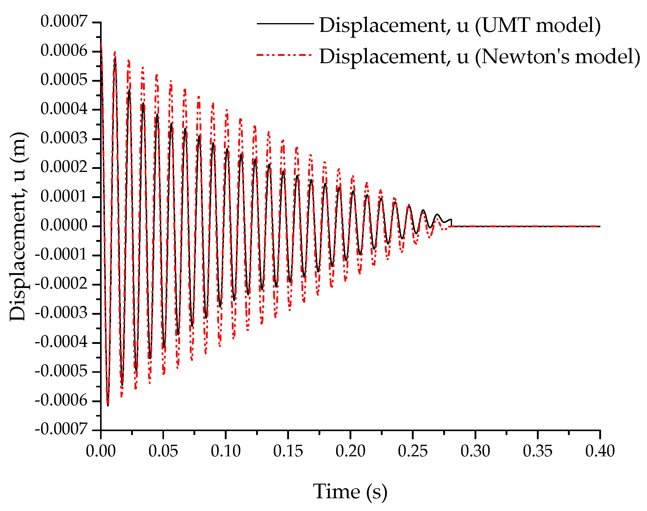
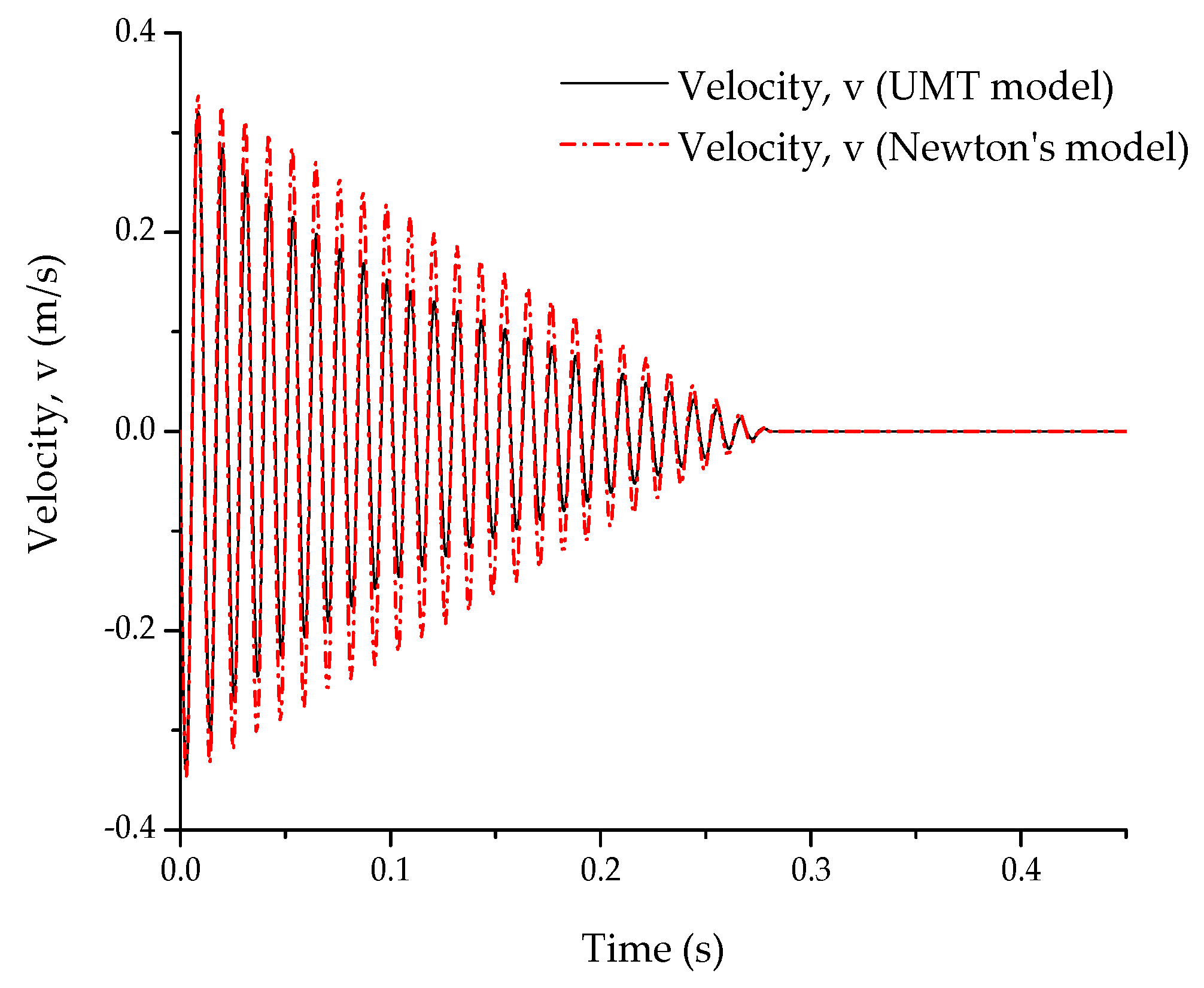
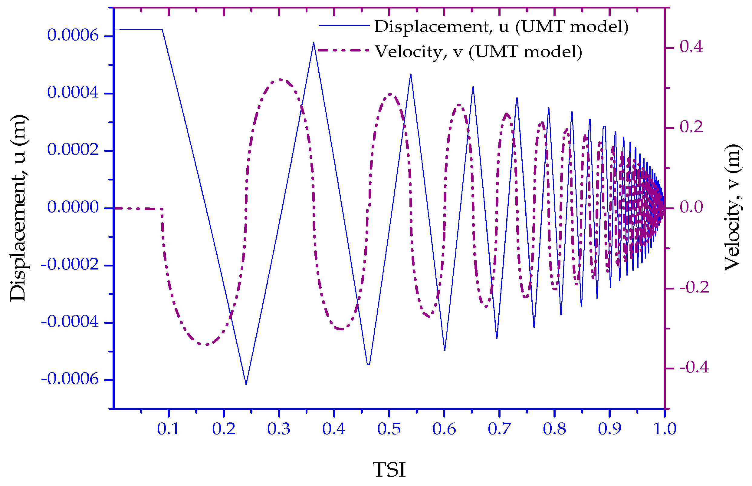
Newtonian mechanics equilibrium Equation (35) and unified mechanics equilibrium Equation (39) were solved for an initial excitation. Results are plotted in Figure 3 through Figure 6 for the input parameters given in Table 1. The solution of the equation of motion in unified mechanics theory and Newton’s law for damped oscillation of the mass are shown in Figure 3 for displacement and Figure 4 for velocity, respectively. It can be readily noticed that both models capture damped oscillation. However, the decay in amplitude is linear for Newton’s model, and in unified mechanics, the response is nonlinear. Experimental results on similar models [39,41] show that the amplitude decay is not linear. Since the response of the mass-spring system in the unified mechanics equilibrium equation is dependent on the entropy evolution within the system, a detailed study is required to get the entropy generation function, also known as thermodynamic fundamental equation. However, the current study is limited to the derivation of the governing equation using the fundamental principles of unified mechanic theory on a dissipative system and limit to a macroscopic (experimental level) model for dissipation at the friction-contact interface, as given in Equation (38).

Figure 5 shows the response of mass-spring oscillator subjected friction, along the TSI axis. In the present context, the TSI axis represents the thermodynamic state of oscillation. Hence, the interpretation of TSI in the present study is limited to the dissipation of strain energy stored in the spring. As shown in Figure 5, the oscillations dampen and the strain energy and kinetic energy of the mass-spring system decays. Even though the Newtonian equation of motion given in Equation (35) for the mass-spring system takes care of damping due to friction, the equation does not directly deal with the thermodynamics of the energy dissipation. However, the unified mechanics theory accounts for the thermodynamics of the system, in the equation of motion, as derived in Equation (34). Dynamic equilibrium Equation (34) in unified mechanics theory accounts for all the dissipative processes in an entropy generation function.

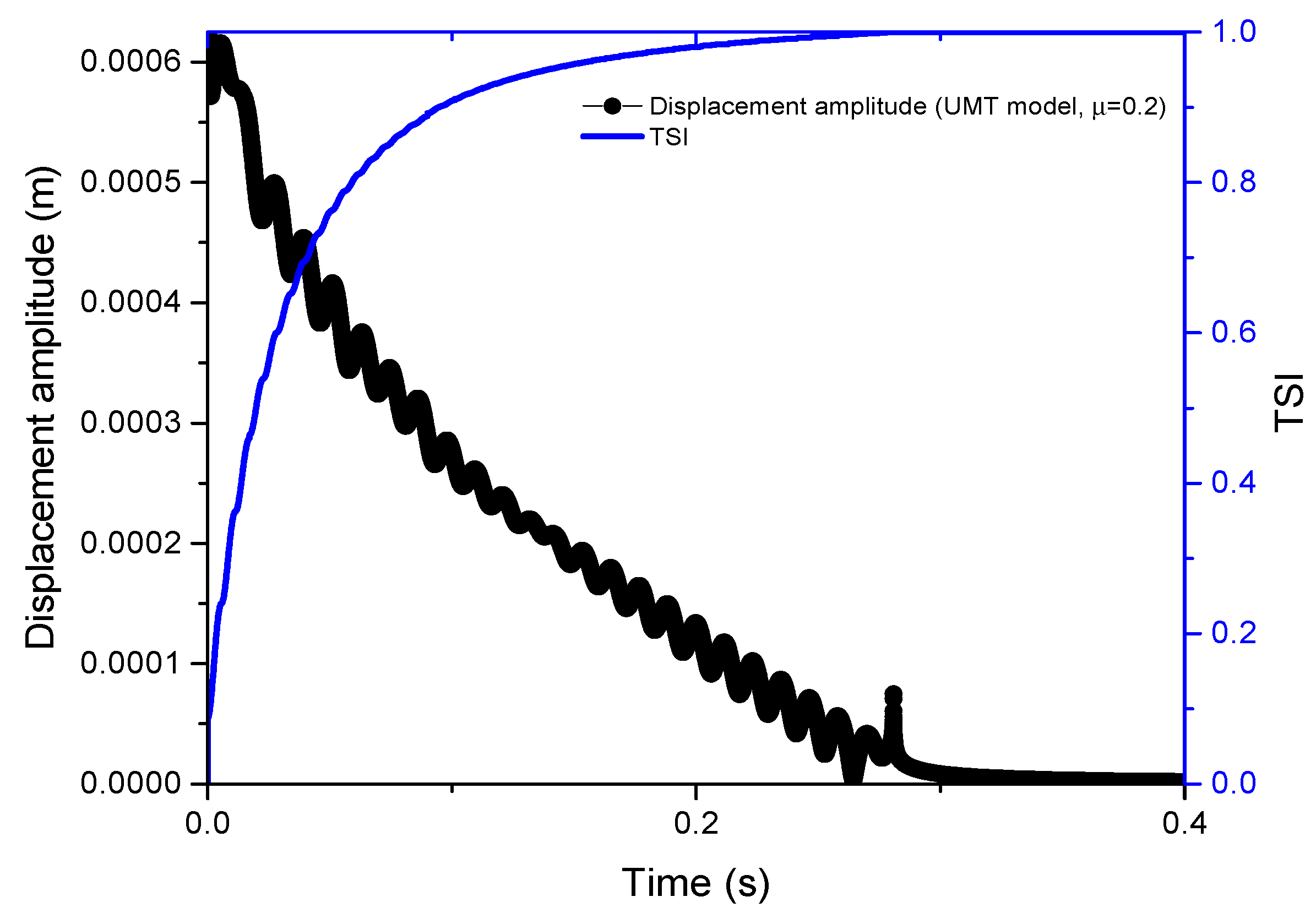
Unified mechanics theory (UMT) [9] proposes a space-time-TSI coordinate system [9,10]. Figure 6 shows the results from the present study, for the space-time-TSI relation of the damped oscillation under friction. Such a relationship cannot be obtained by Newton’s equations unless the laws of thermodynamics are invoked separately. Even if they are invoked separately, in Newton’s equations, the derivative of entropy with respect to displacement is zero, which is obviously not correct. Amplitude variations for the model parameters listed in Table 1 are oscillatory as shown Figure 6. This is due to the numerical error in the approximation of the solution of the differential equation given in Equation (34) using Newmark’s method. Since the present study is not focused on the numerical accuracy of the solution techniques, exploration of other methods of numerical techniques are excluded from the present study. The similarity in the trends of TSI plotted for the various physical systems [9] including the mass-spring system in the present study, is due to the statistical nature of Boltzmann’s equation for entropy, from which the unified mechanic theory is based on [8].

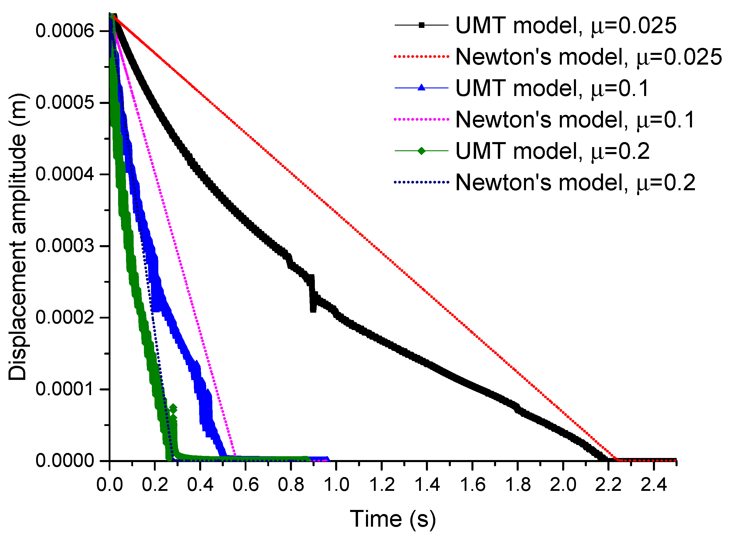
The linearity of amplitude decay in the Newtonian equation of motion for friction is not observed in experiments and in the unified mechanics theory-based formulation, as shown in Figure 7. From Figure 7, one can readily notice that the rate of amplitude decay is constant for the Newtonian mechanics equation. Nevertheless, tangents to the curves in Figure 7 would show that the rate of amplitude decay in the unified mechanics theory-based model is high in the initial stage of oscillation when compared with the final stage. This could be due to the macro-level model approximations for the entropy generation equation proposed in Equation (38). A separate detailed study is required for the identification of all the entropy generation sources that are active in the contact surfaces of the friction block model. Such a study can help in reproducing the nonlinear response of friction block experiments [39,41].

Figure 7 shows the variation in amplitudes of vibration for the mass-spring system with different frictional coefficients. The unified mechanics theory captures the time at which oscillation stops, as predicted by using the Newtonian mechanics equation. All the results using the proposed model show numerical errors in the solution. Since the objective of this study is limited to the derivation of the governing equation of motion in unified mechanics theory and to compare the results with that of the Newtonian mechanics equation of motion, various aspects of numerical solution techniques are excluded from the present study.

5.2. Comparison with Experimental Data

An experimental data set published in the literature [46] is used to compare the predictions using the dynamic equilibrium Equation (39) in the unified mechanics’ theory (UMT) and Newton’s equilibrium Equation (35). The experimental setup consists of a mass-spring single degree of freedom system with dry friction [46] subjected to an initial displacement. A linear voltage differential transformer is used to sense the motion of mass [46]. A combined effect of Coulomb friction and viscous damping on a single degree of freedom system is investigated by using a similar experimental setup [47]. A list of the model parameters used in this comparative study is given in

Table 2. List of parameters used to compare the proposed model and the Newtonian mechanics equation with experimental data.

Parameter	Value	Unit
Spring stiffness,$\mathrm{k}$ [47]	$54$	N/m
Critical TSI, ${\mathsf{\Phi }}_{\mathrm{c}}$	1	-
$\mathrm{Thermodynamic} \mathrm{friction} \mathrm{coefficient}, \mathsf{\lambda }$	0.003	-
Mass, $\mathrm{m}$ [47]	1.51	kg
Sliding friction coefficient, $\mathsf{\mu }$ [47]	$4.23\times {10}^{-4}$	-
Molar mass for iron, ${\mathrm{m}}_{\mathrm{s}}$	$55.84\times {10}^{-3}$	Kg/mol
Displacement at t = 0, ${\mathrm{u}}_0$	$4.25\times {10}^{-3}$	m

.

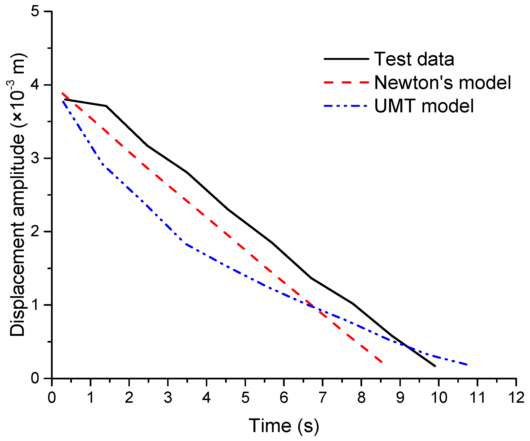
Results are plotted in Figure 8 and Figure 9 by using the input parameters given in Table 2. Model predictions and test data for displacements and displacement-amplitude of vibration are shown in Figure 8 and Figure 9, respectively. As shown in Figure 8, both the unified mechanics’ theory-based model and Newton’s equation of motion capture damped oscillations under Coulomb friction. The amplitude variations, as shown in Figure 9, show a different trend for the unified mechanics theory-based model when compared with the predictions using Newton’s equation of motion. Newton’s equation of motion predicts closer results to the test data [47]. However, it is to be noted that Newton’s model parameter involves an experimental curve-fit data, representing the frictional force. Nevertheless, the unified mechanics theory-based model involves TSI, which evolves with the thermodynamics of dissipative mechanisms that are associated with friction. In other words, Newton’s model captures a dissipative process under friction, without considering the thermodynamics of the vibration.

From Figure 8 and Figure 9, it can be seen that the amplitude decay is not exactly linear in the dry-friction experiment [47]. It can also be noticed in the test data [47] that the mean position at the end of oscillation deviates from the initial equilibrium position of the mass by an amplitude of $4.1\times {10}^{-4}$ m. However, the calculated value of the amplitude of displacement of the mass under static equilibrium condition, ${\left|\mathrm{u}\right|}_{\mathrm{static}}=\frac{\mathsf{\mu }\mathrm{mg}}{\mathrm{k}}$ is $1.16\times {10}^{-4}$ m. This could be due to a difference in the spring stiffness in the experimental setup [47] while the mass oscillates in the negative displacement half-cycles, when compared to the stiffness of the spring during the positive displacement half cycles and also due to the damage in the spring due to the mechanical deformation. Since the spring stiffness in the models is constant under both the compressive and tensile loading directions, such a variation cannot be noticed in the model predictions. With the experimental curve-fitted data for frictional coefficient, the results using the solution of Newton’s equilibrium Equation (35) agree with the initial positive peaks of half-cycles of oscillation and do not predict the negative peaks of initial half-cycle data for displacement. While comparing the duration of free vibration in Figure 8, the equilibrium Equation (39) in UMT predicts a close result with the test data. Since the equilibrium equation in UMT is a function of thermodynamic quantity, entropy, the model requires estimation of entropy evolution to get the solution matching with the test data. Linearity or the nonlinearity of the predicted amplitude variation using the equilibrium equation in UMT, is dependent on the thermodynamic fundamental equation in Equation (38). Current scope of the study is to derive and present the dynamic equilibrium equation in UMT. Hence, we limit the application of the derived dynamic equilibrium equation in UMT in a Coulomb friction model using a macroscopic model for entropy generation function at the friction-contact interface, in Equation (38).

6. Conclusions

In this work, we attempted to derive the dynamic equilibrium equations based on the unified mechanics theory for a dissipative free-vibration problem. The generic form of the dynamic equilibrium equations of the unified mechanics theory in terms of Lagrangian for the nonconservative system is presented. Unlike Newtonian mechanics equations, this generic form has a new axis, called the Thermodynamic State Index (TSI) axis in addition to space-time axes. Unlike in the Newtonian mechanics equation such as the one presented in Equation (34), in unified mechanics theory-based Equation (22), the derivative of displacement with respect to TSI is non-zero. The term representing nonconservative force in Equation (22), is dependent on the entropy generation of the system rather than an empirical damping term ‘C’ in the Newtonian mechanics equilibrium equations. Hence the proposed model has a physical basis and does not require empirical curve-fit to the experimental data. However, friction coefficients must be measured experimentally.

The proposed model is applied on a mass-spring single degree of freedom system subjected to friction and the results are compared with that of a Newtonian mechanics formulation.

In unified mechanics theory, in dynamic equilibrium equations all dissipation mechanisms must be included in the thermodynamic fundamental equation. There is no need for an empirical C constant. Hence, the unified mechanics dynamic equilibrium is more fundamental and physics-based than using thermodynamically consistent Newtonian mechanics formulation.

Thermodynamic state index can also be used to model degradation evolution in the spring in the system without any empirical test data. Examples of this are given in references [1,2,3,4,5,6,7,8,9,10,11,12,13,14,15,16]. In Newtonian mechanics, degradation evolution must be introduced by an empirical curve fit.

As shown in Figure 8, ideally the predictions using the Newtonian model Equation (35) with a test data-fitted friction coefficient, match well when compared with the same test data. However, the equilibrium Equation (34) in the unified mechanics theory is a function of the entropy generation, which is not a curve-fitted coefficient. Hence the predictions using Equation (34) are dependent on the form of the thermodynamic fundamental equation for entropy generation. Thermodynamic fundamental Equation (39) for the sliding friction is derived to include mainly the mechanical dissipation. Hence, a separate study is required to incorporate other dissipative processes such as a contact material diffusion, acoustic losses etc., in the thermodynamic fundamental equation and to match the solutions of the unified mechanics’ theory-based dynamic equilibrium equation with the test data.

The dynamic equilibrium Equation (34) can be used in various applications. One of the applications involves one of the oldest scientific topics, the study of the dynamics of pendulum. Under large amplitudes of oscillations, Newton’s model with linear friction is inadequate to model the experimental observations. For this reason, nonlinearities are introduced [48] in the model. Such nonlinearities associated with the dynamic event are governed not only by the mechanics of motion, but also by the thermodynamics involved in it. Hence, the Equation (34) contributes to an approach of thermodynamically consistent modelling of such nonlinearities associated with the motion of pendulum-oscillator, without an extended empirical nonlinear model. Further, the applications of the thermodynamically consistent dynamic equilibrium Equation (35) can be extended to study the friction pendulum dampers used in structural isolations [49,50,51] and other friction dampers used as an energy dissipation devices for structures against an earthquake load [52,53,54]. The dynamic equilibrium equation can also be used for investigating frictional dissipation in vibration energy harvesters [55], independent energy dissipation mechanisms in impact-pendulum [56] and in rub-impact events [57], and influence of wear-dust on contacting surfaces or on the dissipation characteristics etc.

References

- David Halliday; Resnick, R.; Walker, J. Fundamentals of Physics, 9th ed.; John Wiley & Sons: Hoboken, NJ, USA, 2011. [Google Scholar]
- Penchina, C.M. Pseudowork-energy principle. Am. J. Phys. 1978, 46, 295–296. [Google Scholar] [CrossRef]
- Silverberg, J.; Widom, A. Classical analytical mechanics and entropy production. Am. J. Phys. 2007, 75, 993–996. [Google Scholar] [CrossRef] [Green Version]
- Güémez, J.; Fiolhais, M. Dissipation effects in mechanics and thermodynamics. Eur. J. Phys. 2016, 37, 045101. [Google Scholar] [CrossRef] [Green Version]
- Basaran, C. Entropy Based Fatigue, Fracture, Failure Prediction and Structural Health Monitoring. Entropy 2020, 22, 1178. [Google Scholar] [CrossRef] [PubMed]
- Broda, E. Ludwig Boltzmann? Man, physicist, philosopher, biologist. Rheol. Acta 1982, 21, 357–359. [Google Scholar] [CrossRef]
- Boltzmann, L. On the Relation of a General Mechanical Theorem to the Second Law of Thermodynamics. In Kinetic Theory; Elsevier: Amsterdam, The Netherlands, 1966. [Google Scholar]
- Basaran, C.; Yan, C.-Y. A Thermodynamic Framework for Damage Mechanics of Solder Joints. J. Electron. Packag. 1998, 120, 379–384. [Google Scholar] [CrossRef] [Green Version]
- Basaran, C. Introduction to Unified Mechanics Theory with Applications; Springer International Publishing: Berlin/Heidelberg, Germany, 2021. [Google Scholar]
- Bin Jamal M., N.; Kumar, A.; Chebolu, L.R.; Basaran, C. Low Cycle Fatigue Life Prediction Using Unified Mechanics Theory in Ti-6Al-4V Alloys. Entropy 2020, 22, 24. [Google Scholar] [CrossRef] [Green Version]
- Basaran, C.; Nie, S. An Irreversible Thermodynamics Theory for Damage Mechanics of Solids. Int. J. Damage Mech. 2004, 13, 205–223. [Google Scholar] [CrossRef]
- Basaran, C.; Chandaroy, R. Using finite element analysis for simulation of reliability tests on solder joints in microelectronic packaging. Comput. Struct. 2000, 74, 215–231. [Google Scholar] [CrossRef]
- Basaran, C.; Lin, M. Damage mechanics of electromigration induced failure. Mech. Mater. 2008, 40, 66–79. [Google Scholar] [CrossRef]
- Basaran, C.; Lin, M. Damage mechanics of electromigration in microelectronics copper interconnects. Int. J. Mater. Struct. Integr. 2007, 1, 16. [Google Scholar] [CrossRef]
- Li, S.; Abdulhamid, M.F.; Basaran, C. Simulating Damage Mechanics of Electromigration and Thermomigration. Simulation 2008, 84, 391–401. [Google Scholar] [CrossRef]
- Gomez, J.; Basaran, C. Damage mechanics constitutive model for Pb/Sn solder joints incorporating nonlinear kinematic hardening and rate dependent effects using a return mapping integration algorithm. Mech. Mater. 2006, 38, 585–598. [Google Scholar] [CrossRef]
- Tang, H.; Basaran, C. A Damage Mechanics-Based Fatigue Life Prediction Model for Solder Joints. J. Electron. Packag. 2003, 125, 120–125. [Google Scholar] [CrossRef]
- Basaran, C.; Zhao, Y.; Tang, H.; Gomez, J. A Damage-Mechanics-Based Constitutive Model for Solder Joints. J. Electron. Packag. 2004, 127, 208–214. [Google Scholar] [CrossRef]
- M, N.B.J.; Rao, C.L.; Basaran, C. A unified mechanics theory-based model for temperature and strain rate dependent proportionality limit stress of mild steel. Mech. Mater. 2021, 155, 103762. [Google Scholar] [CrossRef]
- Basaran, C.; Nie, S. A thermodynamics based damage mechanics model for particulate composites. Int. J. Solids Struct. 2007, 44, 1099–1114. [Google Scholar] [CrossRef] [Green Version]
- Gomez, J.; Lin, M.; Basaran, C. Damage Mechanics Modeling of Concurrent Thermal and Vibration Loading on Electronics Packaging. Multidiscip. Model. Mater. Struct. 2006, 2, 309–326. [Google Scholar] [CrossRef]
- Gomez, J.; Basaran, C. Nanoindentation of Pb/Sn solder alloys; experimental and finite element simulation results. Int. J. Solids Struct. 2006, 43, 1505–1527. [Google Scholar] [CrossRef] [Green Version]
- Mostaghel, N.; Davis, T. Representations of Coulomb Friction for Dynamic Analysis. Earthq. Eng. Struct. Dyn. 1997, 26, 541–548. [Google Scholar] [CrossRef]
- Stewart, D.E. Rigid-Body Dynamics with Friction and Impact. SIAM Rev. 2000, 42, 3–39. [Google Scholar] [CrossRef] [Green Version]
- Quinn, D.D. A New Regularization of Coulomb Friction. J. Vib. Acoust. 2004, 126, 391–397. [Google Scholar] [CrossRef]
- Andreaus, U.; Casini, P. Dynamics of Friction Oscillators Excited by a Moving base and/or Driving Force. J. Sound Vib. 2001, 245, 685–699. [Google Scholar] [CrossRef]
- Shiryaev, V.; Orlik, J. A one-dimensional computational model for hyperelastic string structures with Coulomb friction. Math. Methods Appl. Sci. 2016, 40, 741–756. [Google Scholar] [CrossRef]
- Shiryaev, V.; Neusius, D.; Orlik, J. Extension of One-Dimensional Models for Hyperelastic String Structures under Coulomb Friction with Adhesion. Lubrication 2018, 6, 33. [Google Scholar] [CrossRef] [Green Version]
- Champneys, A.R.; Várkonyi, P.L. The Painlevé paradox in contact mechanics. IMA J. Appl. Math. 2016, 81, 538–588. [Google Scholar] [CrossRef] [Green Version]
- Nosonovsky, M.; Breki, A.D. Ternary Logic of Motion to Resolve Kinematic Frictional Paradoxes. Entropy 2019, 21, 620. [Google Scholar] [CrossRef] [Green Version]
- Preclik, T.; Rüde, U. Numerical Experiments with the Painlevé Paradox: Rigid Body vs. Compliant Contact. In Proceedings of the Joint International Conference on Multibody System Dynamics, Stuttgart, Germany, 29 May–1 June 2012. [Google Scholar]
- Nosonovsky, M. Entropy in Tribology: In the Search for Applications. Entropy 2010, 12, 1345–1390. [Google Scholar] [CrossRef]
- Amiri, M.; Khonsari, M.M. On the Thermodynamics of Friction and Wear―A Review. Entropy 2010, 12, 1021–1049. [Google Scholar] [CrossRef] [Green Version]
- Marion, J.B. Hamilton’s Principle—Lagrangian and Hamiltonian Dynamics. In Classical Dynamics of Particles and Systems; Elsevier: Amsterdam, The Netherlands, 1965; pp. 214–266. [Google Scholar]
- E Musielak, Z. Standard and non-standard Lagrangians for dissipative dynamical systems with variable coefficients. J. Phys. A Math. Theor. 2008, 41, 41. [Google Scholar] [CrossRef] [Green Version]
- Lazo, M.J.; Krumreich, C.E. The action principle for dissipative systems. J. Math. Phys. 2014, 55, 122902. [Google Scholar] [CrossRef] [Green Version]
- Martínez-Pérez, N.E.; Ramirez, C. On the Lagrangian description of dissipative systems. J. Math. Phys. 2018, 59, 032904. [Google Scholar] [CrossRef] [Green Version]
- Szegleti, A.; Márkus, F. Dissipation in Lagrangian Formalism. Entropy 2020, 22, 930. [Google Scholar] [CrossRef]
- Torzo, G.; Peranzoni, P. The Real Pendulum: Theory, Simulation, Experiment. Latin-American J. Phys. Educ. 2009, 3, 221–228. [Google Scholar]
- Marino, L.; Cicirello, A. Experimental investigation of a single-degree-of-freedom system with Coulomb friction. Nonlinear Dyn. 2020, 99, 1781–1799. [Google Scholar] [CrossRef] [Green Version]
- Onorato, P.; Mascoli, D.; DeAmbrosis, A. Damped oscillations and equilibrium in a mass-spring system subject to sliding friction forces: Integrating experimental and theoretical analyses. Am. J. Phys. 2010, 78, 1120–1127. [Google Scholar] [CrossRef]
- Knopoff, L.; Macdonald, G.J.F. Models for acoustic loss in solids. J. Geophys. Res. Space Phys. 1960, 65, 2191–2197. [Google Scholar] [CrossRef]
- Uday, M.B.; Fauzi, M.N.A.; Zuhailawati, H.; Ismail, A.B. Advances in friction welding process: A review. Sci. Technol. Weld. Join. 2010, 15, 534–558. [Google Scholar] [CrossRef]
- Newmark, N.M. A Method of Computation for Structural Dynamics. J. Eng. Mech. Div. 1959, 85, 67–94. [Google Scholar] [CrossRef]
- Lindfield, G.; Penny, J. Solution of Differential Equations. In Numerical Methods, 4th ed.; Academic Press: Cambridge, MA, USA, 2019; ISBN 9780128122563. [Google Scholar]
- Feeny, B.; Liang, J. A decrement method for the simultaneous estimation of coulomb and viscous friction. J. Sound Vib. 1996, 195, 149–154. [Google Scholar] [CrossRef]
- Liang, J.-W. Identifying Coulomb and viscous damping from free-vibration acceleration decrements. J. Sound Vib. 2005, 282, 1208–1220. [Google Scholar] [CrossRef]
- Leven, R.; Koch, B. Chaotic behaviour of a parametrically excited damped pendulum. Phys. Lett. A 1981, 86, 71–74. [Google Scholar] [CrossRef]
- Nedelcu, D.; Iancu, V.; Gillich, G.-R.; Bogdan, S.L. Study on the effect of the friction coefficient on the response of structures isolated with friction pendulums. Vibroeng. Procedia 2018, 19, 6–11. [Google Scholar] [CrossRef]
- Nedelcu, D.; Malin, C.-T.; Gillich, G.-R.; Petrica, A.; Padurean, I. Comparison of the performance of friction pendulums with uniform and variable radii. Vibroengineering Procedia 2019, 23, 81–86. [Google Scholar] [CrossRef]
- Hong, X.; Guo, W.; Wang, Z. Seismic Analysis of Coupled High-Speed Train-Bridge with the Isolation of Friction Pendulum Bearing. Adv. Civ. Eng. 2020, 2020, 1–15. [Google Scholar] [CrossRef]
- Min, K.-W.; Seong, J.-Y.; Kim, J. Simple design procedure of a friction damper for reducing seismic responses of a single-story structure. Eng. Struct. 2010, 32, 3539–3547. [Google Scholar] [CrossRef]
- Ribakov, Y. Semi-active predictive control of non-linear structures with controlled stiffness devices and friction dampers. Struct. Des. Tall Spéc. Build. 2004, 13, 165–178. [Google Scholar] [CrossRef]
- Seong, J.-Y.; Min, K.-W.; Kim, J.-C. Analytical investigation of an SDOF building structure equipped with a friction damper. Nonlinear Dyn. 2012, 70, 217–229. [Google Scholar] [CrossRef]
- Nammari, A.; Caskey, L.; Negrete, J.; Bardaweel, H. Fabrication and characterization of non-resonant magneto-mechanical low-frequency vibration energy harvester. Mech. Syst. Signal Process. 2018, 102, 298–311. [Google Scholar] [CrossRef]
- Witelski, T.; Virgin, L.; George, C. A driven system of impacting pendulums: Experiments and simulations. J. Sound Vib. 2014, 333, 1734–1753. [Google Scholar] [CrossRef]
- Huang, Z.; Tan, J.; Liu, C.; Lu, X. Dynamic Characteristics of a Segmented Supercritical Driveline with Flexible Couplings and Dry Friction Dampers. Symmetry 2021, 13, 281. [Google Scholar] [CrossRef]
Figure 2.
Block diagram of a mass-spring system subjected to friction.
Figure 3.
Position versus time for a damped oscillator in the presence of contact surface friction.
Figure 4.
Velocity versus time for a damped oscillator in the presence of contact surface friction.
Figure 5.
The response of mass-spring oscillator along with the Thermodynamic State Index (TSI) axis.
Figure 6.
Change in the amplitude of oscillation and evolution of TSI with time for frictional dissipation.
Figure 7.
Amplitude versus time for various values of frictional coefficients.
Figure 8.
Comparison between model predictions and test data [47] for the displacement versus time data.
Figure 9.
Comparison between the model predictions and test data [47] for the amplitude versus time data.