Polyhedral DC Decomposition and DCA Optimization of Piecewise Linear Functions


Institut für Mathematik, Humboldt-Universität zu Berlin, 10099 Berlin, Germany
*
Author to whom correspondence should be addressed.
Algorithms 2020, 13(7), 166; https://0-doi-org.brum.beds.ac.uk/10.3390/a13070166
Submission received: 28 May 2020
/
Revised: 5 July 2020
/
Accepted: 8 July 2020
/
Published: 11 July 2020
(This article belongs to the Special Issue Nonsmooth Optimization in Honor of the 60th Birthday of Adil M. Bagirov)
Abstract
:For piecewise linear functions we show how their abs-linear representation can be extended to yield simultaneously their decomposition into a convex and a concave part , including a pair of generalized gradients . The latter satisfy strict chain rules and can be computed in the reverse mode of algorithmic differentiation, at a small multiple of the cost of evaluating f itself. It is shown how and can be expressed as a single maximum and a single minimum of affine functions, respectively. The two subgradients and are then used to drive DCA algorithms, where the (convex) inner problem can be solved in finitely many steps, e.g., by a Simplex variant or the true steepest descent method. Using a reflection technique to update the gradients of the concave part, one can ensure finite convergence to a local minimizer of f, provided the Linear Independence Kink Qualification holds. For piecewise smooth objectives the approach can be used as an inner method for successive piecewise linearization.
1. Introduction and Notation
There is a large class of functions that are called DC because they can be represented as the difference of two convex functions, see for example [1,2]. This property can be exploited in various ways, especially for (hopefully global) optimization. We find it notationally and conceptually more convenient to express these functions as averages of a convex and a concave function such that
Throughout we will annotate the convex part by superscript and the concave part by superscript , which seems rather intuitive since they remind us of the absolute value function and its negative. Since we are mainly interested in piecewise linear functions we assume without much loss of generality that the functions f and the convex and concave components are well defined and finite on all of the Euclidean space . Allowing both components to be infinite outside their proper domain would obviously generate serious indeterminacies, i.e., s in the numerical sense. As we will see later we can in fact ensure in our setting that pointwise
which means that we actually obtain an inclusion in the sense of interval mathematics [3]. This is one of the attractions of the averaging notation. We will therefore also refer to and as the concave and convex bounds of f.
Conditioning of the Decomposition
In parts of the literature the two convex functions and are assumed to be nonnegative, which has some theoretical advantages. In particular, see, e.g., [4], one obtains for the square of a DC function f the decomposition
The sign conditions of and are necessary to ensure that the three squares on the right hand side are convex functions. Using the Apollonius identity one may then deduce in a constructive way that not only sums but also products of DC functions inherit this property. In general, since the convex functions and have both supporting hyperplanes one can at least theoretically always find positive coefficients and such that
Then the average of these modified functions is still f and their respective convexity/concavity properties are maintained. In fact, this kind of proximal shift can be used to show that any twice Lipschitz continuously differentiable function is DC, which raises the suspicion that the property by itself does not provide all that much exploitable structure from a numerical point of view. We believe that for its use in practical algorithms one has to make sure or simply assume that the condition number
is not too large. Otherwise, there is the danger that the value of f is effectively lost in the rounding error of evaluating . For sufficiently large quadratic shifts of the nature specified above one has . The danger of an excessive growth in seems akin to the successive widening in interval calculations and similarly stems also from the lack of strict arithmetic rules. For example doubling f and then subtracting it yields the successive decompositions
If in Equation (3) by chance we had originally so that with the condition number we would get after the doubling and subtraction the condition number . So it is obviously important that the original algorithm avoids as much as possible calculations that are ill-conditioned in that they even just partly compensate each other.
Throughout the paper we assume that the functions in question are evaluated by a computational procedure that generates a sequence of intermediate scalars, which we denote generically by and w. The last one of these scalar variables is the dependent, which is usually denoted by f. All of them are continuous functions of the vector of independent variables. As customary in mathematics we will often use the same symbol to identify a function and its dependent variable. For the overall objective we will sometimes distinguish them and write . For most of the paper we assume that the intermediates are obtained from each other by affine operations or the absolute value function so that the resulting are all piecewise linear functions.
The paper is organized as follows. In the following Section 2 we develop rules for propagating the convex/concave decomposition through a sequence of abs-linear operations applied to intermediate quantities u. This can be done either directly on the pair of bounds or on their average u and their halved distance . In Section 3 we organize such sequences into an abs-linear form for f and then extend it to simultaneously yield the convex/concave decomposition. As a consequence of this analysis we get a strengthened version of the classical representation of piecewise linear functions, which reduces to the difference of two polyhedral parts in max- and min-form. In Section 4 we develop strict rules for propagating certain generalized gradient pairs of exploiting convexity and the cheap gradient principle [5]. In Section 5 we discuss the consequences for the DCA when using limiting gradients , solving the inner, linear optimization problem (LOP) exactly, and ensuring optimality via polyhedral reflection. In Section 6 we demonstrate the new results on the nonconvex and piecewise linear chained Rosenbrock version of Nesterov [6]. Section 7 contains a summary and preliminary conclusion with outlook. In the Appendix A we give the details of the necessary and sufficient optimality test from [7] in the present DC context.
2. Propagating Bounds and/or Radii
In Equation (3) we already assumed that doubling is done componentwise and that for a difference of DC functions w and u, one defines the convex and concave parts by
respectively. This yields in particular for the negation
For piecewise linear functions we need neither the square formula Equation (2) nor the more general decompositions for products. Therefore we will not insist on the sign conditions even though they would be also maintained automatically by Equation (4) as well as the natural linear rules for the convex and concave parts of the sum and the multiple of a DC function, namely
However, the sign conditions would force one to decompose simple affine functions as
which does not seem such a good idea from a computational point of view.
The key observation for this paper is that as is well known (see e.g., [8]), one can propagate the absolute value operation according to the identity
Here the equality in the second line can be verified by shifting the difference into the two arguments of the max. Again we see that when applying the absolute value operation to an already positive convex function we get and so that the condition number grows from to . In other words, we observe once more the danger that both component functions drift apart. This looks a bit like simultaneous growth of numerator and denominator in rational arithmetic, which can sometimes be limited through cancelations by common integer factors. It is currently not clear when and how a similar compactification of a given convex/concave decomposition can be achieved. The corresponding rule for the maximum is similarly easy derived, namely
When u and w as well as their decomposition are identical we arrive at the new decomposition , which obviously represents again some deterioration in the conditioning.
While it was pointed out in [4] that the DC functions themselves form an algebra, their decomposition pairs are not even an additive group, as only the zero has a negative partner, i.e., an additive inverse. Naturally, the pairs form the Cartesian product between the convex cone of convex functions and its negative, i.e., the cone of concave functions. The DC functions are then the linear envelope of the two cones in some suitable space of locally Lipschitz continuous functions. It is not clear whether this interpretation helps in some way, and in any case we are here mainly concerned with piecewise linear functions.
Propagating the Center and Radius
Rather than propagating the pairs through an evaluation procedure as defined in [5] to calculate the function value at a given point x, it might be simpler and better for numerical stability to propagate the pair
This representation resembles the so-called central form in interval arithmetic [9] and we will call therefore u the central value and the radius. In other words, u is just the normal piecewise affine intermediate function and the is a convex distance function to the hopefully close convex and concave part. Should the potential blow-up discussed above actually occur, this will only effect but not the central value u itself. Moreover, at least theoretically one might decide to reduce from time to time making sure of course that the corresponding and as defined in Equation (7) stay convex and concave, respectively. The condition number now satisfies the bound
Recall here that all intermediate quantities are functions of the independent variable vector . Naturally, we will normally only evaluate the intermediate pairs u and at a few iterates of whatever numerical calculation one performs involving f so that we can only sample the ratio
pointwise, where the denominator is hopefully nonzero. We will also refer to this ratio as the relative gap of the convex/concave decomposition at a certain evaluation point x. The arithmetic rules for propagating radii of the central form in central convex/concave arithmetic are quite simple.
Lemma 1 (Propagation rules for central form).
Withtwo constants and an independent variable we have
Proof.
The last rule follows from Equation (6) by
☐
The first equation in Equation (8) means that for all quantities u that are affine functions of the independent variables x the corresponding radius is zero so that until we reach the first absolute value. Notice that does indeed grow additively for the subtraction just like for the addition. By induction it follows from the rules above for an inner product that
where the are assumed to be constants. As we can see from the bounds in Lemma 1 the relative gap can grow substantially whenever one performs an addition of values with opposite sign or applies the absolute value operation. In contrast to interval arithmetic on smooth functions one sees that the relative gap, though it may be zero or small initially immediately jumps above 1 when one hits the first absolute value operation. This is not really surprising since the best concave lower bound on itself is so that , and thus constantly. On the positive side one should notice that throughout we do not lose sight of the actual central values , which can be evaluated with full arithmetic precision. In any case we can think of neither nor as small numbers, but we must be content if they do not actually explode too rapidly. Therefore they will be monitored throughout our numerical experiments.
Again we see that the computational effort is almost exactly doubled. The radii can be treated as additional variables that occur only in linear operations and stay nonnegative throughout. Notice that in contrast to the (nonlinear) interval case we do not loose any accuracy by propagating the central form. It follows immediately by induction from Lemma 1 that any function evaluated by a evaluation procedure that comprises a finite sequence of
- initializations to independent variables
- multiplications by constants
- additions or subtractions
- absolute value applications
is piecewise affine and continuous. We will call these operations and the resulting evaluation procedure abs-linear. It is also easy to see that the absolute values can be replaced by the maximum or the minimum or the positive part function or any combination of them, since they can all be mutually expressed in terms of each other and some affine operations. Conversely, it follows from the min-max representation established in [10] (Proposition 2.2.2) that any piecewise affine function f can be evaluated by such an evaluation procedure. Consequently, by applying the formulas Equations (4)–(6) one can propagate at the same time the convex and concave components for all intermediate quantities. Alternatively, one can propagate the centered form according to the rules given in Lemma 1. These rules are also piecewise affine so that we have a finite procedure for simultaneously evaluating and or u and as piecewise linear functions. The combined computation requires about 2–3 times as many arithmetic operations and twice as many memory accesses. Of course due to the interdependence of the two components it is not possible to evaluate just one of them without the other. As we will see the same is true for the generalized gradients to be discussed later in Section 4.
3. Forming and Extending the Abs-Linear Form
In practice all piecewise linear objectives can be evaluated by a sequence of abs-linear operations, possibly after min and max have been rewritten as
Our only restriction is that the number s of intermediate scalar quantities, say , is fixed, which is true for example in the representation. Then we can immediately cast the procedure in matrix-vector notation as follows:
Lemma 2 (Abs-Linear Form).
Any continuous piecewise affine functioncan be represented by
wherestrictly lower triangular,anddenotes the componentwise modulus of the vector z.
It should be noted that the construction of this general abs-linear form requires no analysis or computation whatsoever. However, especially for our purpose of generating a reasonably tight DC decomposition, it is advantages to reduce the size of the abs-normal form by eliminating all intermediates with for which never occurs on the right hand side. To this end we may simply substitute the expression of given in the j-th row in all places where itself occurs on the right hand side. The result is what we will call a reduced abs-normal form, where after renumbering, all remaining with are switching variables in that occurs somewhere on the right hand side. In other words, all but the last column of the reduced, strictly lower triangular matrix L are nontrivial. Again, this reduction process is completely mechanical and does not require any nontrivial analysis, other than looking up which columns of the original L were zero. The resulting reduced system is smaller and probably denser, which might increase the computation effort for evaluating f itself. However, in view of Equation (9) we must expect that for the reduced form the radii will grow slower if we first accumulate linear coefficients and then take their absolute values. Hence we will assume in the remainder of this paper that the abs-normal form for our objective f of interest is reduced.
Based on the concept of abs-linearization introduced in [11], a slightly different version of a (reduced) abs-normal form was already proposed in [12]. Now in the present paper, both z and y depend directly on z via the matrix M and the vector b, but y does no longer depend directly on . All forms can be easily transformed into each other by elementary modifications. The intermediate variables can be calculated successively for by
where , and denote the ith rows of the corresponding matrix. By induction on i one sees immediately that they are piecewise affine functions , and we may define for each x the signature vector
Consequently we get the inverse images
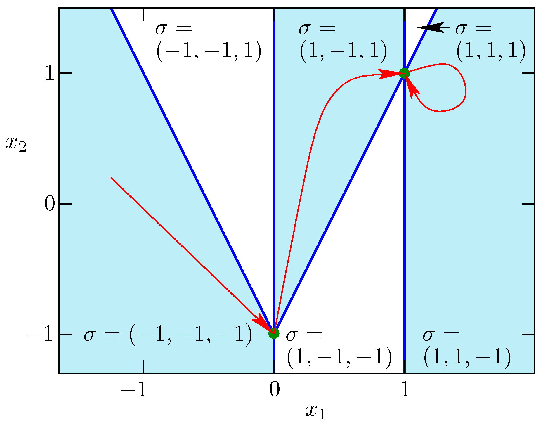
which are relatively open polyhedra that form collectively a disjoint decomposition of . The situation for the second example of Nesterov is depicted in Figure 3 in the penultimate section. There are six polyhedra of full dimension, seven polyhedra of co dimension 1 drawn in blue and two points, which are polyhedra of dimension 0. The point with signature is stationary and the point with signature is the minimizer as shown in [7]. The arrows indicate the path of our reflection version of the DCA method as described in Section 5.
When is definite, i.e., has no zero components, which we will denote by , it follows from the continuity of that has full dimension n unless it is empty. In degenerate situations this may also be true for indefinite but then the closure of is equal to the extended closure
for some definite . Here the (reflexive) partial ordering ≺ between the signature vectors satisfies the equivalence
as shown in [13]. One can easily check that for any there exists a unique signature
We call the reflection of at , which satisfies also and we have in fact . Hence the relation between and is symmetric in that also . Therefore we will call a complementary pair with respect to . In the very special case for the are orthants and their reflections at the origin are their geometric opposites with . Here one can see immediately that all edges, i.e., one-dimensional polyhedra, have Cartesian signatures for and belong to or for any given . Notice that is a local minimizer of a piecewise linear function if and and only if it is a local minimizer along all edges of nonsmoothness emanating form it. Consequently, optimality of f restricted to a complementary pair is equivalent to local optimality on , not only in this special case, but whenever the Linear Independence Kink Qualification (LIKQ) holds as introduced in [13] and defined in the Appendix A. This observation is the basis of the implicit optimality condition verified by our DCA variant Algorithm 1 through the use of reflections. The situation is depicted in Figure 3 where the signatures and as well as and form complementary pairs at and , respectively. At both reflection points there are four emanating edges, which all belong to one of the three polyhedra mentioned.
Applying the propagation rules from Lemma 1, one obtains with the recursion
where the modulus is once more applied componentwise for vectors and matrices. Hence, we have again in matrix vector notation
which yields for the explicit expression
Here, is the so-called switching depth of the abs-linear form of f, namely the largest such that , which is always less than s due to the strict lower triangularity of M and L. The unit lower triangular is an M-matrix [14], and interestingly enough does not even depend on x but directly maps to . For the radius of the function itself, the propagation rules from Lemma 1 then yield
Theorem 1 (Inclusion by convex/concave decomposition).
For any piecewise affine function f in abs-linear form, the construction defined in Section 2 yields a convex/concave inclusion
Moreover, the convex and the concave partsandhave exactly the same switching structure asin that they are affine on the same polyhedradefined in (13).
Proof.
It follows from Equation (17) that the radii are like the piecewise linear with the only nonsmoothness arising through the switching variables themselves. Obviously this property is inherited by and the linear combinations and , which completes the proof. ☐
Combining Equations (16) and (18) with the abs-linear form of the piecewise affine function f and defining , one obtains for the calculation of the following abs-linear form
with the vectors and matrices defined by
Then, Equations (19) and (20) yield
i.e., Equations (16) and (18). As can be seen, the matrices and have the required strictly lower triangular form. Furthermore, it is easy to check, that the switching depth of the abs-linear form of f carries over to the abs-linear form for in that also . However, notice that this system is not reduced since the s radii are not switching variables, but globally nonnegative anyhow. We can now obtain explicit expressions for the central values, radii, and bounds for a given signature .
Corollary 1 (Explicit representation of the centered form).
For any definite signatureand allwe have with
where the restrictions of the functions and their gradients toare denoted by subscript σ. Notice that the gradients are constant on these open polyhedra.
Proof.
As one can see the computation of the gradient requires the solution of one unit upper triangular linear system and that of both and one more. Naturally, upper triangular systems are solved by back substitution, which corresponds to the reverse mode of algorithmic differentiation as described in the following section. Hence, the complexity for calculating the gradients is exactly the same as that for calculating the functions, which can be obtained by one forward substitution for and an extra one for and thus and . The given and are proper gradients in the interior of the full dimensional domains . For some or even many the inverse image of the map may be empty, in which case the formulas in the corollary do not apply. Checking the nonemptiness of for a given signature amounts to checking the consistency of a set of linear inequalities, which costs the same as solving an LOP and is thus nontrivial. Expressions for the generalized gradients at points in lower dimensional polyhedra are given in the following Section 4. There it is also not required that the abs-linear normal form has been reduced, but one may consider any given sequence of abs-linear operations.
The Two-Term Polyhedral Decomposition
It is well known ([15], Theorem 2.49) that all piecewise linear and globally convex or concave functions can be represented as the maximum or the minimum of a finite collection of affine functions, respectively. Hence, from the convex/concave decomposition we get the following drastic simplification of the classical min-max representation given, e.g., in [10].
Corollary 2 (Additive max/min decomposition of PL functions).
For every piecewise affine functionthere existaffine functionsforandaffine functions for such that at all
where furthermore .
The max-part of this representation is what is called a polyhedral function in the literature [15]. Since the min-part is correspondingly the negative of a polyhedral function we may also refer to Equation (26) as a DP decomposition, i.e., the difference of two polyhedral functions.
We are not aware of a publication that gives a practical procedure for computing such a collection of affine functions , , and , , for a given piecewise linear function f. Of course the critical question is in which form the function f is specified. Here as throughout our work we assume that it is given by a sequence of abs-linear operations. Then we can quite easily compute for each intermediate variable v representations of the form
with index sets and since one has to consider all possibilities of selecting one affine function each from one of the max and min groups, respectively. Obviously, (28) involves and affine function terms in contrast to the first representation (27) which contains just and of them. Still the second version conforms to the classical representation of convex and concave piecewise linear functions, which yields the following result:
Corollary 3 (Explicit computation of the DP representation).
For any piecewise linear function given as abs-linear procedure one can explicitly compute the representation (26) by implementing the rules of Lemma 1.
Proof.
We will consider the representations (27) from which (26) can be directly obtained in the form (28). Firstly, the independent variables are linear functions of themselves with gradient and inhomogeneity . Then for multiplications by a constant we have to scale all affine functions by c. Secondly, addition requires appending the expansions of the two summands to each other without any computation. Taking the negative requires switching the sign of all affine functions and interchanging the max and min group. Finally, to propagate through the absolute values we have to apply the rule (6), which means switching the signs in the min group, expressing it in terms of max and merging it with the existing max group. Here merging means pairwise joining each polyhedral term of the old max-group with each term in the switched min-group. Then the new min-group is the old one plus the old max-group with its sign switched. ☐
We see that taking the absolute value or, alternatively, maxima or minima generates the strongest growth in the number of polyhedral terms and their size. It seems clear that this representation is generally not very useful because the number of terms will likely blow up exponentially. This is not surprising because we will need one affine function for each element of the polyhedral decompositions of the domain of the max and min term. Typically, many of the affine terms will be redundant, i.e., could be removed without changing the values of the polyhedral terms. Unfortunately, identifying those already requires solving primal or dual linear programming problems, see, e.g., [16]. It seems highly doubtful that this would ever be worthwhile. Therefore, we will continue to advocate dealing with piecewise linear functions in a convenient procedural abs-linear representation.
4. Computation of Generalized Gradients and Constructive Oracle Paradigm
For optimization by variants of the DCA algorithm [17] one needs generalized gradients of the convex and the concave component. Normally, there are no strict rules for propagating generalized gradients through nonsmooth evaluation procedures. However, exactly this is simply assumed in the frequently invoked oracle paradigm, which states that at any point the function value and an element can be evaluated. We have argued in [18] that this is not at all a reasonable assumption.
On the other hand, it is well understood that for the convex operations: Positive scaling, addition, and taking the maximum the rules are strict and simple. Moreover, then the generalized gradient in the sense of Clarke is actually a subdifferential in that all its elements define supporting hyperplanes. Similarly might be called a superdifferential in that the tangent planes bound the concave part from above.
In other words, we have at all and for all increments
and
which imply for and that
where the lower bound on the left is a concave function and the upper bound is convex, both with respect to . Notice that the generalized superdifferential being the negative of the subdifferential of is also a convex set.
Now the key question is how we can calculate a suitable pair of generalized gradients . As we noted above the convex part and the negative of the concave part only undergo convex operations so that for
and for
Finally, for we find by Equation (6) that as well as
where we have used that in Equation (32). The sign of the arguments u of the absolute value function are of great importance, because they determine the switching structure. For this reason, we formulated the cases in terms of u rather than in the convex/concave components. The operator denotes taking the convex hull or envelope of a given usually closed set. It is important to state that within an abs-linear representation the multipliers c will stay constant independent of the argument x, even if they were originally computed as partial derivatives by an abs-linearization process and thus subject to round-off error. In particular their sign will remain fixed throughout whatever algorithmic calculation we perform involving the piecewise linear function f. So, actually the case could be eliminated by dropping this term completely and just initializing the left hand side v to zero.
Because we have set identities we can propagate generalized gradient pairs and perform the indicated algebraic operations on them, starting with the Cartesian basis vectors
The result of this propagation is guaranteed to be an element of . Recall that in the merely Lipschitz continuous case generalized gradients cannot be propagated with certainty since for example the difference generates a proper inclusion . In that vein we must emphasize that the average need not be a generalized gradient of as demonstrated by the possibility that algebraically but we happen to calculate different generalized gradients of and at a particular point x. In fact, if one could show that one would have verified the oracle paradigm, whose use we consider unjustified in practice. Instead, we can formulate another corollary for sufficiently piecewise smooth functions.
Definition 1.
For any, the set of functionsdefined by an abs-normal form
withand, is denoted by
Once more, this definition differs slightly from the one given in [7] in that y depends only on z
and not on |z| in order to match the abs-linear form used here. Then one can show the following result:
Corollary 4 (Constructive Oracle Paradigm).
For any functionand a given point x there exist a convex polyhedral functionand a concave polyhedral functionsuch that
Moreover, both terms and their generalized gradients ator anywhere else can be computed with the same order of complexity as f itself.
Proof.
In [11], we show that
where is a piecewise linearization of f developed at x and evaluated at Applying the convex/concave decomposition of Theorem 1, one obtains immediately the assertion with a convex polyhedral function and a concave polyhedral function evaluated at The complexity results follow from the propagation rules derived so far. ☐
We had hoped that it would be possible to use this approximate decomposition into polyhedral parts to construct at least locally an exact decomposition of a general function into a convex and compact part. The natural idea seems to add a sufficiently large quadratic term to
such that it would become convex. Then the same term could be subtracted from maintaining its concavity. Unfortunately, the following simple example shows that this is not possible.
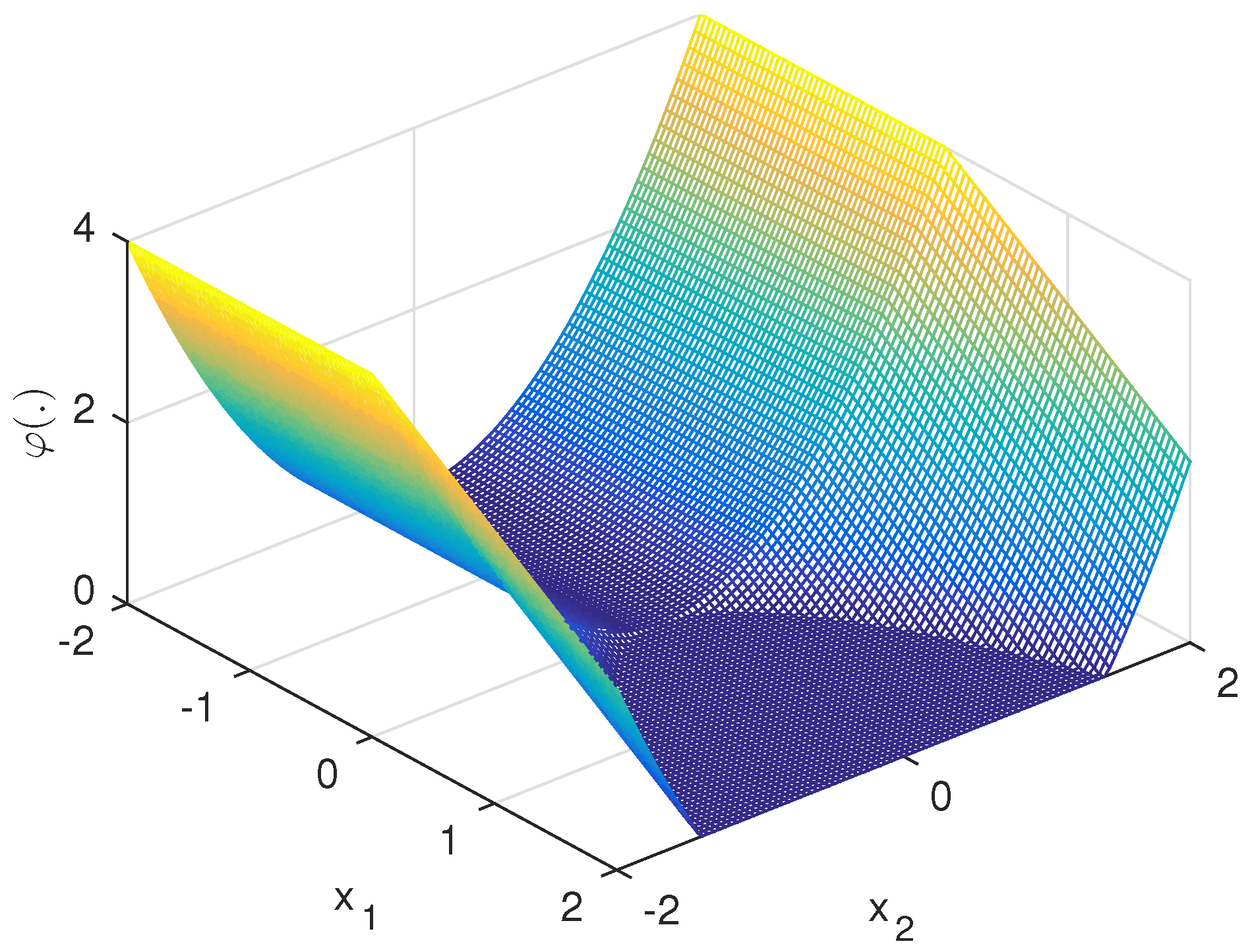
Example 1 (Half pipe).
The function
in the classis certainly nonconvex as shown in Figure 1. As already observed in [19] this generally nonsmooth function is actually Fréchet differentiable at the origin x = 0 with a vanishing gradient Hence, we have and may simply choose constantly However, neither by adding nor any other smooth function to can we eliminate the downward facing kink along the vertical axis In fact, it is not clear whether this example has any DC decomposition at all.
Applying the Reverse Mode for Accumulating Generalized Gradients
Whenever gradients are propagated forward through a smooth evaluation procedure, i.e., for functions in , they are uniquely defined as affine combinations of each other, starting from Cartesian basis vectors for the components of x. Given only the coefficients of the affine combinations one can propagate corresponding adjoint values, or impact factors backwards, to obtain the gradient of a single dependent with respect to all independents at a small multiple of the operations needed to evaluate the dependent variable by itself. This cheap gradient result is a fundamental principle of computational mathematics, which is widely applied under various names, for example discrete adjoints, back propagation, and reverse mode differentiation. For a historical review see [20] and for a detailed description using similar notation to the current paper see our book [5]. For good reasons, there has been little attention to the reverse mode in the context of nonsmooth analysis, where one can at best obtain subgradients. The main obstacle is again that the forward propagation rules are only sharp when all elementary operations maintain convexity, which is by the way the only constructive way of verifying convexity for a given evaluation procedure. While general affine combinations and the absolute value are themselves convex functions, they do not maintain convexity when applied to a convex argument.
The last equation of Lemma 1 shows that one cannot directly propagate a subgradient of the convex radius functions because there is a reference to itself, which does not maintain convexity except when it is redundant due to its argument having a constant sign. However, it follows from the identity that for all intermediates u
Hence one can get affine lower bounds of the radii, although one would probably prefer upper bounds to limit the discrepancy between the convex and concave parts. When and we may choose according to Equation (32) any convex combination
It is tempting but not necessarily a good idea to always choose the weight μ equal to for simplicity.
Before discussing the reasons for this at the end of this subsection, let us note that from the values of the constants c, the intermediate values u, and the chosen weights μ it is clear how the next generalized gradient pair is computed as a linear combination of the generalized gradients of the inputs for each operation, possibly with a switch in their roles. That means after only evaluating the function f itself, not even the bounds and , we can compute a pair of generalized gradients in using the reverse mode of algorithmic differentiation, which goes back to at least [21] though not under that name. The complexity of this computation will be independent of the number of variables and relative to the complexity of the function f itself. All the operations are relatively benign, namely scaling by constants, interchanges and additions and subtractions. After all the reverse mode is just a reorganization of the linear algebra in the forward propagation of gradients. Hence, it appears that we can be comparatively optimistic regarding the numerical stability of this process.
To be specific we will indicate the (scalar) adjoint value of all intermediates and as usual by and . They are all initialized to zero except for either or . Then at the end of the reverse sweep, the vectors represent either or , respectively. For computational efficiency one may propagate both adjoint components simultaneously, so that one computes with sextuplets consisting of and their adjoints with respect to and . In any case we have the following adjoint operations. For
for
and finally for
Of course, the update for the critical case of the absolute value is just the convex combination for the two cases and weighted by μ. Due to round-off errors it is very unlikely that the critical case ever occurs in floating point arithmetic. Once more, the sign of the arguments u of the absolute value function are of great importance, because they determine on which faces of the polyhedral functions and the current argument x is located. In some situations one prefers a gradient that is limiting in that it actually occurs as a proper gradient on one of the adjacent smooth pieces. For example, if we had simply for and chose we would get and find by Equation (34) that at . This is not a limiting gradient of
since , whose interior contains the particular generalized gradient 0.
5. Exploiting the Convex/concave Decomposion for the DC Algorithm
In order to minimize the decomposed objective function f we may use the DCA algorithm [17] which is given in its basic form using our notation by
where denotes the Fenchel conjugate of . For a convex function one has
see [15], Chapter 11. Hence, the classic DCA reduces in our Euclidean scenario to a simple recurrence
The objective function on the left hand side is a constantly shifted convex polyhedral upper bound on since
It follows from Equation (29) and being a minimizer that
Now, since (36) is an LOP, an exact solution can be found in finitely many steps, for example by a variant of the Simplex method. Moreover, we can then assume that is one of finitely many vertex points of the epigraph of . At these vertex points, f itself attains a finite number of bounded values. Provided f itself is bounded below, we can conclude that for any choice of the the resulting function values can only be reduced finitely often so that and w.l.o.g. eventually. We then choose the next with as the reflection of at as defined in (15). If then again it follows from Corollary A2 that is a local minimizer of f and we may terminate the optimization run. Hence we obtain the DCA variant listed in Algorithm 1, which is guaranteed to reach local optimality under LIKQ. It is well defined even without this property and we conjecture that otherwise the final iterate is still a stationary point of f. The path of the algorithm on the example discussed in Section 5 is sketched in Figure 3. It reaches the stationary point where from within the polyhedron with the signature and then continues after the reflection . From within that polyhedron the inner loop reaches the point with signature , whose minimality is established after a search in the polyhedron .
If the function is unbounded below, so will be one of the inner convex problems and the convex minimizer should produce a ray of infinite descent instead of the next iterate . This exceptional scenario will not be explicitly considered in the remainder of the paper. The reflection operation is designed to facilitate further descent or establish local optimality. It is discussed in the context of general optimality conditions in the following subsection.
| Algorithm1 Reflection DCA |
Require:
|
5.1. Checking Optimality Conditions
Stationarity of happens when the convex function is minimal at so that for all large k
The nonemptiness condition on the right hand side is known as criticality of the DC decomposition at , which is necessary but not sufficient even for local optimality of at . To ensure the latter one has to verify that all satisfy the criticality condition (38) so that
The left inclusion is a well known local minimality condition [22], which is already sufficient in the piecewise linear case. The right inclusion is equivalent to the left one due to the convexity of .
If and were unrelated convex and concave polyhedral functions, one would normally consider it extremely unlikely that were nonsmooth at any one of the finitely many vertices of the polyhedral domain decomposition of . For instance when is smooth at we find that is a singleton so that criticality according to Equation (38) is already sufficient for local minimality according to Equation (39). As we have seen in Theorem 1 the two parts have exactly the same switching structure. That means they are nonsmooth on the same skeleton of lower dimensional polyhedra. Hence, neither nor will be singletons at minimizing vertices of the upper bound so that checking the validity of Equation (39) appears to be a combinatorial task at first sight.
However, provided the Linear Independence Kink Qualification (LIKQ) defined in [7] is satisfied at the candidate minimizer , the minimality can be tested with cubic complexity even in case of a dense abs-linear form. Moreover, if the test fails one can easily calculate a descent direction d. The details of the optimality test in our context including the calculation of a descent direction are given in the Appendix A. They differ slightly from the ones in [7]. Rather than applying the optimality test Proposition A1 explicitly, one can use its Corollary A2 stating that if with is a local minimizer of the restriction of f to a polyhedron with definite then it is a local minimizer of the unrestricted f if and only if it also minimizes the restriction of f to with the reflection . The latter condition must be true if also minimizes , which can be checked by solving that convex problem. If that test fails the optimization can continue.
5.2. Proximal Rather Than Global
By some authors the DCA algorithm has been credited with being able to reach global minimizers with a higher probability than other algorithms. There is really no justification for this optimism in the light of the following observation. Suppose the objective has an isolated local minimizer . Then there exists an such that the level set has a bounded connected component containing , say . Now suppose DCA is started from any point . Since is by Equation (37) a convex upper bound on its level set will be contained in . Hence any step from that reduces the upper bound must stay in the same component, so there is absolutely no chance to move away from the catchment of towards another local minimizer of f, whether global or not. In fact, by adding the convex term
which vanishes at , to the actual objective one performs a kind of regularization, like in the proximal point method. This means the step is actually held back compared to a larger step that might be taken by a method that only requires the reduction of itself.
Hence we may interpret DCA as a proximal point method where the proximal term is defined as an affinely shifted negative of the concave part. Since in general the norm and the coefficient defining the proximal term may be quite hard to select, this way of defining it may make a lot of sense. However, it is certainly not global optimization. Notice that in this argument we have used neither the polyhedrality nor the inclusion property. So it applies to a general DC decomposition on Euclidean space. Another conclusion from the "holding back" observation is that it is probably not worthwhile to minimize the upper bound very carefully. One might rather readjust the shift after a few or even just one iteration.
6. Nesterov’s Piecewise Linear Example
According to [6], Nesterov suggested three Rosenbrock-like test functions for nonsmooth optimization. One of them given by
is nonconvex and piecewise linear. It is shown in [6] that this function has Clarke stationary points only one of which is a local and thus the global minimizer. Numerical studies showed that optimization algorithms tend to be trapped at one of the stationary points making it an interesting test problem. We have demonstrated in [23] that using an active signature strategy one can guarantee convergence to the unique minimizer from any starting point albeit using in the worst case iterations as all stationary points are visited. Let us first write the problem in the new abs-linear form.
Defining the switching variables
and
the resulting objective function is then simply identical to . With the vectors and matrices
where Z and L have different row partitions, one obtains an abs-linear form (11) of f. Here, denotes the identity matrix of dimension k, the vector containing only ones and the symbol 0 pads with zeros to achieve the specified dimensions. One can easily check that , hence this example has switching depth . The geometry of the situation is depicted in Figure 3, which was already briefly discussed in Section 3 and Section 5.
Since the corresponding extended abs-linear form for does not provide any new insight we do not state it here. Directly in terms of the original equations we obtain for the radii
and
Clearly is a concave function and to check the convexity of we note that
The last expression is the sum of an affine function and the positive part of the sum of the absolute value and an affine function, which must therefore also be convex. The corresponding term in Equation (42) is the same with the convex function added, so that is also convex in agreement with the general theory. Finally, one verifies easily that
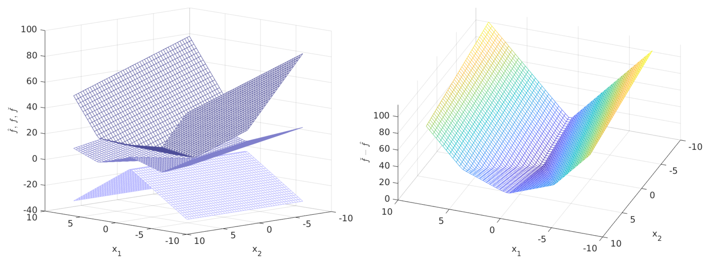
which is the whole idea of the decomposition. It would seem that the automatic decomposition by propagation through the abs-linear procedure yields a rather tight result. The function f as well as the lower and upper bound given by the convex/concave decomposition are illustrated on the left hand side of Figure 2. Notice that the switching structure is indeed identical for all three as stated in Theorem 1. On the right hand side of Figure 2, the difference between the upper, convex and lower, concave bound is shown, which is indeed convex.
It is worthwhile to look at the condition number of the decomposition, namely we get the following trivial bound
The disappointing right hand side value follows from the fact that at the well known unique global optimizer the numerator is zero and the denominator positive. However, elsewhere, we can bound the conditioning as follows.
Lemma 3.
Proof.
Since the denominator is piecewise linear and vanishes only at the minimizer there must be a constant such that for
which takes the value on the boundary. On the other hand we get for and thus in particular
Assuming without loss of generality that we can combine the two bounds to obtain the assertion with . ☐
Hence, we see the condition number is nicely bounded and the decomposition should work as long as our optimization algorithm has not yet reached its goal . It is verified in the companion article [24], that the DCA exploiting the observations made in this paper reaches the global minimizer in finitely many steps. It was already shown in [7] that the LIKQ condition is satisfied everywhere and that the optimality test singles out the unique minimizer correctly. In Figure 3, the arrows indicate the path of our reflection version of the DCA method as described in Section 5.
7. Summary, Conclusions and Outlook
In this paper the following new results were achieved
- For every piecewise linear function f given as an abs-linear evaluation procedure, rules for simultaneously evaluating its representation as the average of a concave lower bound and a convex upper bound are derived.
- The two bounds can be constructively expressed as a single maximum and minimum of affine functions, which drastically simplifies the classical representation. Due to its likely combinatorial complexity we do not recommend this form for practical calculations.
- For the two bounds and , generalized gradients and can be propagated forward or reverse through the convex or concave operations that define them. The gradients are not unique but guaranteed to yield supporting hyperplanes and thus provide a verified version of the oracle paradigm.
- The DCA algorithm can be implemented such that a local minimizer is reached in finitely many iterations, provided the Linear Independence Kink Qualification (LIKQ) is satisfied. It is conjectured that without this assumption the algorithm still converges in finitely many steps to a Clarke stationary point. Details on this can be found in the companion paper [24].
These results are illustrated on the piecewise linear Rosenbrock variant of Nesterov.
On a theoretical level it would be gratifying and possibly provide additional insight, to prove the result of Corollary A3 directly using the explicit representations of the generalized differentials of the convex and concave part given in Corollary 1. Moreover, it remains to be explored what happens when LIKQ is not satisfied. We have conjectured in [25] that just verifying the weaker Mangasarian Fromovitz Kink Qualification (MFKQ) represents an NP hard task. Possibly, there are other weaker conditions that can be cheaply verified and facilitate the testing for at least local optimality.
Global optimality can be characterized theoretically in terms of subgradients, albeit with ε arbitrarily large [26]. There is the possibility that the alternative definition of ε-gradients given in [18] might allow one to constructively check for global optimality. It does not really seem clear how these global optimality conditions can be used to derive corresponding algorithms.
The implementation of the DCA algorithm can be optimized in various ways. Notice that for applying the Simplex method in standard form, one could use for the representation as DC function the max-part in the more economical representation Equation (27) introducing additional variables, rather than the potentially combinatorial Equation (28) to assemble the constraint matrix. In any case it seems doubtful that solving each sub problem to completion is a good idea, especially as the resulting step in the outer iteration is probably much too small anyhow. Therefore, the generalized gradient of the concave part, which defines the inner problem, should probably be updated much more frequently. Moreover, the inner solver might be an SQOP type active signature method or a matrix free gradient method with momentum term, as is used in machine learning, notwithstanding the nonsmoothness of the objective. Various options in that range will be discussed and tested in the companion article [24].
Finally, one should always keep in mind that the task of minimizing a piecewise linear function will most likely occur as an inner problem in the optimization of a piecewise smooth and nonlinear function. As we have shown in [27] the local piecewise linear model problem can be obtained easily by a slight generalization of automatic or algorithmic differentiation, e.g., ADOL-C [28] and Tapenade [29].
Author Contributions
Conceptualization, A.G. and A.W.; methodology, A.G. and A.W.; writing—original draft preparation; writing—review and editing, A.G. and A.W. All authors have read and agreed to the published version of the manuscript.
Funding
We acknowledge support by the German Research Foundation (DFG) and the Open Access Publication Fund of Humboldt-Universität zu Berlin.
Acknowledgments
We thank Napsu Karmitsa and Sona Taheri for inviting us to participate in this special issue in honor of Adil M. Bagirov. We also thank the three anonymous referees, who asked for various corrections and clarifications, which made the paper much more self-contained and readable.
Conflicts of Interest
The authors declare no conflict of interest.
Appendix A. Polynomial Optimality Test Based on Abs-Linear Form
As illustrated for the Nesterov test function, it may be advantageous to use intermediate variables that are not arguments of the absolute value themselves. For simplicity, we assume that these switching variables that do not impose nonsmoothness are located in the last components of z and that only the components are arguments of the absolute value. Let us abbreviate the current iterate with and denote the corresponding switching vector by , the signature vector and the active index set by with cardinality . Consequently, there are exactly definite signatures by and the same number of limiting gradients for the three generalized differentials , and .
For all , the signature is constant and we can use Corollary 1 to define the smooth function
where we have pulled out the unit lower triangular factor such that
For to be contained in the extended closure as defined in Equation (14), it must satisfy the m linear equations
with denoting the ith unit vector in . Thus it is necessary and sufficient for to be a polyhedron of dimension that the Jacobian has full row rank m. This rank condition was introduced as LIKQ in [7] and obviously requires that no more than n switches are active at . As discussed in [7], for the point to be a local minimizer of f it is necessary that it solves the trunk problem
Here is the projection onto the vector components whose indices do not belong to α so the equality constraint combines (A1) and the constraint . Now we get from KKT theory or equivalently LOP duality that is a minimizer on if and only if for some Lagrange multiplier vector
Since we derive that
where . This is a generally overdetermined system of n equations in the m components of . If it is solvable the full multiplier vector is immediately available. Because of the assumed full rank of the Jacobian we have , and if is a vertex in that the tangential stationarity condition (A3) is automatically satisfied.
Now it is necessary and sufficient for local minimality that is also a minimizer of f on all polyhedra with definite . Any such can be written as with structurally orthogonal to such that for we have the matrix equations
Then we can express the for as
with . Now must be the minimizer of f on , i.e., solve the problem
Notice that the inequalities are only imposed on the sign constraints that are active at since the strict inequalities are maintained in a neighborhood of due to the continuity of . Then we get again from KKT theory or equivalently LOP duality that still and for a second multiplier vector the equalities
Multiplying from the right by the projection we find that the conditions (A2) and (A3) must still hold so that λ remains exactly the same. Moreover, multiplying from the right by we get with and after some rearrangement the inequality
Now the key observation is that this condition is linear in Γ and is strongest for the choice for yielding the inequalities
In other words, is a solution of the branch problems (A4) if and only if it is for the worst case where for . When coincidentally we can define arbitrarily. Note that the complementarity condition associated with Equation (A4) is automatically satisfied at for any μ, since by definition of the active index set α. These observations yield immediately:
Proposition A1 (Necessary and sufficient minimality condition).
Assume LIKQ holds in thathas full row rank. Then the pointis a local minimizer of f if and only if we have tangential stationarity in thatbelongs to the range ofand normal growth holds in that.
The verification that LIKQ holds and subsequently the test whether tangential stationarity is satisfied can be based on a QR decomposition of the active Jacobian . The main expense here is the calculation of itself, which requires one forward substitution on for each of n columns of Z and hence at most fused multiply adds. Very likely this effort will already be made by any kind of active set method for reaching the candidate point . Once the multiplier vector λ is obtained the remaining test (A7) for normal growth is almost for free so that we have a polynomial minimality criterion provided LIKQ holds. Otherwise one may assume a weaker generalization of the Mangasarian Fromovitz constrained qualification called MFKQ in [25]. However, we have conjectured in [19] that verifying MFKQ is probably already NP-hard.
Corollary A1 (Descent direction in the nonoptimal case).
Suppose that LIKQ holds. If tangential stationarity is violated there exits some directionsuch thatbut, which implies descent in thatfor. If tangential stationarity holds but normal growth fails there exists at least onewith. Defining, any d satisfyingis a descent direction.
Proof.
In the first case it is clear that for since the components of with indices in α stay zero and the others vary only slightly. Then the directional derivative of at in direction is given by
which proves the first assertion. Otherwise, λ is well defined and we can choose with . Setting with , one obtains for d with that for . On that polyhedron the Lagrange multiplier vector μ is also well defined by Equation (A6) but we have
Then we get the directional derivative of at in direction
where we have used identity (A5). Hence we have again descent, which completes the proof.
☐
Corollary A2 (Optimality via Reflection).
Suppose anwhere LIKQ holds has been reached by minimizingwithfor. Thenis a local minimizer of f onif and only if it is also a minimizer ofwithas defined in (15).
Proof.
By assumption solves one of the branch problems of f itself. Hence we must have tangential stationarity (A5) with the corresponding for . Since we conclude from (A6) that
which implies that
Hence both tangential stationarity and normal growth are satisfied, which completes the proof by Proposition A1 as the converse implication is trivial. ☐
The key conclusion is that if an is the solution of two complementary convex problems it must be locally optimal in the full dimensional space . Hence one can establish local optimality just using the preferred convex solver. If this test fails one naturally obtains descent to function values below until eventually a local minimizer is found.
Equivalence to DC Optimality Condition
Using the explicit expressions given in Lemma 1 we find that (see [18])
where γ ranges over all complements of such that is definite. Similarly we obtain with
the limiting differentials of the convex and the concave part as
Hence we have an explicit representation for the limiting gradients of f as well as its convex and concave part and at . It is easy to see that the minimality condition (A5) requires a to be in the range of so that we have again yielding
We had hoped to be able to derive directly from these expressions that normal growth implies the condition (39), but we have so far not been able to do so. However, we can indirectly derive the following equivalence.
Corollary A3 (First order minimality condition).
Under LIKQ the limiting differentialis contained in the convex hull ofif and only if tangential stationarity and normal growth condition hold according to Proposition A1.
References
- Joki, K.; Bagirov, A.; Karmitsa, N.; Mäkelä, M. A proximal bundle method for nonsmooth DC optimization utilizing nonconvex cutting planes. J. Glob. Optim. 2017, 68, 501–535. [Google Scholar] [CrossRef]
- Tuy, H. DC optimization: Theory, methods and algorithms. In Handbook of Global Optimization; Springer: Boston, MA, USA, 1995; pp. 149–216. [Google Scholar]
- Rump, S. Fast and parallel interval arithmetic. BIT 1999, 39, 534–554. [Google Scholar] [CrossRef]
- Bačák, M.; Borwein, J. On difference convexity of locally Lipschitz functions. Optimization 2011, 60, 961–978. [Google Scholar]
- Griewank, A.; Walther, A. Evaluating Derivatives: Principles and Techniques of Algorithmic Differentiation; Society for Industrial and Applied Mathematics: Philadelphia, PA, USA, 2008. [Google Scholar]
- Gürbüzbalaban, M.; Overton, M. On Nesterov’s nonsmooth Chebyshev-Rosenbrock functions. Nonlinear Anal. Theory Methods Appl. 2012, 75, 1282–1289. [Google Scholar]
- Griewank, A.; Walther, A. First and second order optimality conditions for piecewise smooth objective functions. Optim. Methods Softw. 2016, 31, 904–930. [Google Scholar] [CrossRef]
- Strekalovsky, A. Local Search for Nonsmooth DC Optimization with DC Equality and Inequality Constraints. In Numerical Nonsmooth Optimization. State of the Art Algorithms; Springer Nature Switzerland AG: Cham, Switzerland, 2020; pp. 229–261. [Google Scholar]
- Hansen, E. (Ed.) The centred form. In Topics in Interval Analysis; Oxford University Press: Oxford, UK, 1969; pp. 102–105. [Google Scholar]
- Scholtes, S. Introduction to Piecewise Differentiable Functions; Springer: New York, NY, USA, 2012. [Google Scholar]
- Griewank, A. On Stable Piecewise Linearization and Generalized Algorithmic Differentiation. Optim. Methods Softw. 2013, 28, 1139–1178. [Google Scholar] [CrossRef]
- Griewank, A.; Bernt, J.U.; Radons, M.; Streubel, T. Solving piecewise linear equations in abs-normal form. Linear Algebra Appl. 2015, 471, 500–530. [Google Scholar] [CrossRef]
- Griewank, A.; Walther, A.; Fiege, S.; Bosse, T. On Lipschitz optimization based on gray-box piecewise linearization. Math. Program. Ser. A 2016, 158, 383–415. [Google Scholar] [CrossRef]
- Golub, G.; Van Loan, C. Matrix Computations, 4th ed.; Johns Hopkins University Press: Baltimore, MD, USA, 2013. [Google Scholar]
- Rockafellar, R.; Wets, R.B. Variational Analysis; Springer: Berlin/Heidelberg, Germany, 1998. [Google Scholar]
- Fukuda, K.; Gärtner, B.; Szedlák, M. Combinatorial redundancy detection. Ann. Oper. Res. 2018, 265, 47–65. [Google Scholar] [CrossRef] [Green Version]
- Le Thi, H.; Pham Dinh, T. DC programming and DCA: Thirty years of developments. Math. Program. Ser. B 2018, 169, 5–68. [Google Scholar] [CrossRef]
- Griewank, A.; Walther, A. Beyond the Oracle: Opportunities of Piecewise Differentiation. In Numerical Nonsmooth Optimization. State of the Art Algorithms; Springer: Cham, Switzerland, 2020; pp. 331–361. [Google Scholar]
- Walther, A.; Griewank, A. Characterizing and testing subdifferential regularity in piecewise smooth optimization. SIAM J. Optim. 2019, 29, 1473–1501. [Google Scholar] [CrossRef]
- Griewank, A. Who invented the reverse mode of differentiation? Doc. Math. 2012, 389–400. [Google Scholar]
- Linnainmaa, S. Taylor expansion of the accumulated rounding error. BIT 1976, 16, 146–160. [Google Scholar] [CrossRef]
- Sun, W.; Sampaio, R.; Candido, M. Proximal point algorithm for minimization of DC function. J. Comput. Math. 2003, 21, 451–462. [Google Scholar]
- Griewank, A.; Walther, A. Finite convergence of an active signature method to local minima of piecewise linear functions. Optim. Methods Softw. 2019, 34, 1035–1055. [Google Scholar] [CrossRef]
- Griewank, A.; Walther, A. The True Steepest Descent Methods Revisited; Technical Report; Humboldt-Universität zu Berlin: Berlin, Germany, 2020. [Google Scholar]
- Griewank, A.; Walther, A. Relaxing kink qualifications and proving convergence rates in piecewise smooth optimization. SIAM J. Optim. 2019, 29, 262–289. [Google Scholar] [CrossRef] [Green Version]
- Niu, Y. Programmation DC & DCA en Optimisation Combinatoire et Optimisation Polynomiale via les Techniques de SDP. Ph.D. Thesis, INSA Rouen, Rouen, France, 2010. [Google Scholar]
- Fiege, S.; Walther, A.; Kulshreshtha, K.; Griewank, A. Algorithmic differentiation for piecewise smooth functions: A case study for robust optimization. Optim. Methods Softw. 2018, 33, 1073–1088. [Google Scholar] [CrossRef]
- Walther, A.; Griewank, A. Getting Started with ADOL-C. In Combinatorial Scientific Computing; Chapman & Hall/CRC Computational Science Series; CRC Press: Boca Raton, FL, USA, 2012; pp. 181–202. [Google Scholar]
- Hascoët, L.; Pascual, V. The Tapenade Automatic Differentiation tool: Principles, Model, and Specification. ACM Trans. Math. Softw. 2013, 39, 20:1–20:43. [Google Scholar]
Figure 1.
Half pipe example as defined in Equation (33).

Figure 2.
Nesterov–Rosenbrock test function polyhedral inclusion for .

Figure 3.
Signatures and reflection-based DCA for Nesterov–Rosenbrock variant (40) with .
Figure 3.
Signatures and reflection-based DCA for Nesterov–Rosenbrock variant (40) with .

© 2020 by the authors. Licensee MDPI, Basel, Switzerland. This article is an open access article distributed under the terms and conditions of the Creative Commons Attribution (CC BY) license (http://creativecommons.org/licenses/by/4.0/).
Share and Cite
MDPI and ACS Style
Griewank, A.; Walther, A. Polyhedral DC Decomposition and DCA Optimization of Piecewise Linear Functions. Algorithms 2020, 13, 166. https://0-doi-org.brum.beds.ac.uk/10.3390/a13070166
AMA Style
Griewank A, Walther A. Polyhedral DC Decomposition and DCA Optimization of Piecewise Linear Functions. Algorithms. 2020; 13(7):166. https://0-doi-org.brum.beds.ac.uk/10.3390/a13070166
Chicago/Turabian StyleGriewank, Andreas, and Andrea Walther. 2020. "Polyhedral DC Decomposition and DCA Optimization of Piecewise Linear Functions" Algorithms 13, no. 7: 166. https://0-doi-org.brum.beds.ac.uk/10.3390/a13070166
Note that from the first issue of 2016, this journal uses article numbers instead of page numbers. See further details here.