Sampling Effects on Algorithm Selection for Continuous Black-Box Optimization


1
School of Mathematics and Statistics, The University of Melbourne, Parkville, VIC 3010, Australia
2
School of Computer and Information Systems, The University of Melbourne, Parkville, VIC 3010, Australia
*
Author to whom correspondence should be addressed.
Algorithms 2021, 14(1), 19; https://0-doi-org.brum.beds.ac.uk/10.3390/a14010019
Submission received: 9 November 2020
/
Revised: 24 December 2020
/
Accepted: 6 January 2021
/
Published: 11 January 2021
(This article belongs to the Special Issue Benchmarking, Selecting and Configuring Learning and Optimization Algorithms)
Abstract
:In this paper, we investigate how systemic errors due to random sampling impact on automated algorithm selection for bound-constrained, single-objective, continuous black-box optimization. We construct a machine learning-based algorithm selector, which uses exploratory landscape analysis features as inputs. We test the accuracy of the recommendations experimentally using resampling techniques and the hold-one-instance-out and hold-one-problem-out validation methods. The results demonstrate that the selector remains accurate even with sampling noise, although not without trade-offs.
1. Introduction
A significant challenge in continuous optimization is to quickly find a target solution to a problem lacking algebraic expressions, calculable derivatives or a well-defined structure. For such black-box problems, the only reliable information available is the set of responses to a group of candidate solutions. Bound-constrained, single-objective, continuous Black-Box Optimization (BBO) problems arise in domains such as science and engineering [1]. Topologically, these problems can have local and global optima, large quality fluctuations between adjacent solutions, and inter-dependencies among variables. Such problem characteristics are typically unknown. Furthermore, BBO problems commonly involve computationally intensive simulations. Hence, finding a target solution is difficult and expensive.
Automated algorithm selection and configuration [2,3,4,5,6,7] solves this problem by constructing a machine learning model that uses Exploratory Landscape Analysis (ELA) features [8] as inputs, where the output is a recommended algorithm. To calculate the ELA features, a sample of candidate solutions must be estimated. Since performance is measured in terms of the number of function evaluations, the added cost of extracting the features must be low enough to avoid significant drops in performance. Precise features are obtained as the sample size increases [9,10,11,12,13,14]; hence, approximated features are used in practice [5,6,7,15]. However, even these successful works acknowledge that with small sample sizes, feature convergence cannot be guaranteed and uncertainty on their values can exist.
There is limited literature exploring the reliability of approximated features. In [16], we explored the effect that translations had on the features, when the cost function is bound-constrained, demonstrating that translations led to phase transitions; hence, providing evidence of non-generality of the features across instances. Renau et al. [17] explored the robustness of the features against the random sampling, number of sample points, and the expressiveness in terms of ability to discriminate problems. Focusing on a fixed dimension of five and seven feature sets, they determined that most features are not robust against the sampling. Saleem et al. [12] proposed a method to evaluate features based on a ranking of similar problems and Analysis of Variance (ANOVA), which does not require machine learning models or confounding experimental factors. Focusing on 12 features, four benchmark sets in two- and five-dimensions, and four one-dimensional transformed functions, they identified that some features effectively capture certain characteristics of the landscape. Moreover, they emphasize the necessity to examine the variability of a feature with different sample sizes, as some can be estimated with small sizes, while others not. Škvorc et al. [13] used ELA to develop a generalized method for visualizing a set of arbitrary optimization functions, focusing on two- and ten-dimensional functions. By applying feature selection, they showed that many features are redundant, and most are non-invariant to simple transformations such as scaling and shifting. Then, Renau et al. [18] identified that the choice of sample generator influences the convergence of the features, depending on their space-covering characteristics. Finally, in more recent work [14], we explored the reliability of five well-known ELA feature sets on a larger set of dimensions, across multiple sample sizes, using a systematic experimental methodology combing exploratory and statistical validation stages, which statistical significance tests and resampling techniques to minimize the computational costs. The results showed that some features are highly volatile for particular functions and sample sizes. In addition, a feature may have significantly different values between two instances of a function due to the bounds of the input space. This implies that the results from an instance should not be generalized across all instances. Moreover, the results show evidence of a curse of the modality, which means that the sample size should increase with the number of local optima in the function.
However, none of these works explore the effect that uncertainty on the features has on the performance of automated algorithm selectors. In this paper, we examine this issue by constructing an automated algorithm selector based on a multi-class, cost-sensitive Random Forest (RF) classification model, which weighted each observation according to the difference in performance between algorithms. We validated our selector on new instances of observed and unobserved problems, achieving good performance with relatively small sample sizes. Then, using resampling strategies, we estimate the systemic error on the selector, demonstrating that randomness in the sample has a minor effect on the accuracy. These results demonstrate that as long as the features are informative, and have low variability, the systemic error on the selector will be small. This conclusion is the main contribution of our paper. The data generated from our experiments has been collected and is available in the LEarning and OPtimization Archive of Research Data (LEOPARD) v1.0 [19].
The remainder of the paper is organized as follows: Section 2 describes the continuous BBO problem and its characteristics using the concepts of fitness landscape, neighborhood, and basin of attraction. In addition, this section describes the algorithm selection framework [20] on which the selector is based. Section 3 presents the components of the selector. Section 4 describes the implementation and validation procedure. We present the results in Section 6. Finally, Section 7 concludes the paper with a discussion of the findings and the limitations of this work.
2. Background and Related Work
2.1. Black-Box Optimization and Fitness Landscapes
Before describing the methods employed, let us define our notation. Without losing generality over maximization, we assume minimization throughout this paper. The goal in a bound-constrained, single-objective, continuous black-box optimization problem is to minimize a cost function where is the input space, is the output space, and is the dimensionality of the problem. A candidate solution is a D-dimensional vector, and the scalar is the candidate’s cost. A continuous BBO problem is the one such that f is unknown; the gradient information is unavailable or uninformative; and there is a lack of specific goals or solution paths. Only the inputs and the outputs of the function are reliable information, and they are analyzed without considering the internal workings of the function. Therefore, a target solution, , is found by sampling the input space.
To find a target solution we may use a search algorithm, which is a systematic procedure that takes previous candidates and their cost as inputs, and generates new and hopefully less costly candidates as outputs. For this purpose, the algorithm maintains a simplified model of the relationship between solutions and costs. The model assumes that the problem has an exploitable structure. Hence, the algorithm can infer details about the structure of the problem by collecting information during the run. We call this structure fitness landscape [21], which is defined as the tuple , where d denotes a distance metric that quantifies the similarity between candidates in the input space. Similar candidates are those where the distance between each one of them is less than a radius [22], forming a neighborhood, , which defines associations between the candidates in the input space.
A local optimum is a candidate such that for all . We denote the set of local optima as . The global optimum for a landscape is a candidate such that for all . We denote the set of global optima as . A fitness landscape can be described using the cardinality of and . An unimodal landscape is the one such that . A multimodal landscape is the one such that . A closely related concept is smoothness, which refers to the magnitude of the change in cost between neighbors. A landscape can be informally classified as rugged, smooth, or neutral. A rugged landscape has large cost fluctuations between neighbors. It presents several local optima and steep ascents and descents. A neutral landscape has large flat areas or plateaus, where changes in the input fail to generate significant changes in the output. At these extremes, both gradient and correlation values are uninformative [23].
The set of local optima can constitute a pattern known as the global structure, which can be used to guide the search for . If the global structure is smooth, it may provide exploitable information. If the global structure is rugged or nonexistent, finding an optimum can be challenging, even impossible [24]. It is also possible to find problems that exhibit deceptiveness, i.e., the global structure and gradient information leads the algorithm away from an optimum, resulting in a performance similar to a random search [23].
A landscape can also be described using its basins of attraction, which is the subset of in which a local search always converges to the same local optimum. The shape of the basins of attraction is a key attribute of the fitness landscape. Landscapes with isotropic or spherical basins have a uniform gradient direction. Landscapes with anisotropic or non-spherical basins are the result of non-uniform variable scaling. This means that changes in one variable result in smaller changes in cost compared to changes in other variables. A successful search in such landscapes requires a small change over one variable and a large change in the others. Anisotropic basins might be non-elliptical. These problems cannot be broken into smaller problems of lower dimensionality, each of which is easier to solve [24]. These problems are non-separable.
In summary, the concepts of basin of attraction, neighborhood and fitness landscape are useful to describe the characteristics of a given optimization problem. The characteristics can be described qualitatively when the structure of the function is known, using descriptors such as rugged or unimodal [24]. On the other hand, the characteristics of the function are unknown in a BBO problem. In addition, the only information available for black-box problems is the set of candidate solutions and their cost values. As such, data-driven methods are the only approach to acquire appropriate knowledge about the structure of the landscape.
A search algorithm should produce in finite time. However, the algorithm may converge prematurely, generating candidates in a small area without finding . This effect is a direct consequence of the model the algorithm maintains of the problem, which is a hard coded bias in the algorithm [25]. The impact that the problem characteristics have on algorithm performance is significant [26]. Both theoretical and experimental studies demonstrate that each algorithm exploits the problem structure differently. As a consequence, no algorithm can solve all possible problems with the best performance [27]. In addition, the relationship between problem structure and algorithm performance is unclear. Furthermore, the significant algorithmic diversity compromises our ability to deeply understand all reported algorithms. Consequently, practitioners may find the algorithm selection stage to be a stumbling block. Most likely, a practitioner will select and adjust/modify one or two algorithms—including their parameters—hoping to obtain the best performance. However, unless the hard coded bias in the algorithm matches the landscape characteristics, we misplace computational resources and human effort. Ideally, we should use an automatic algorithm selection framework.
2.2. The Algorithm Selection Framework
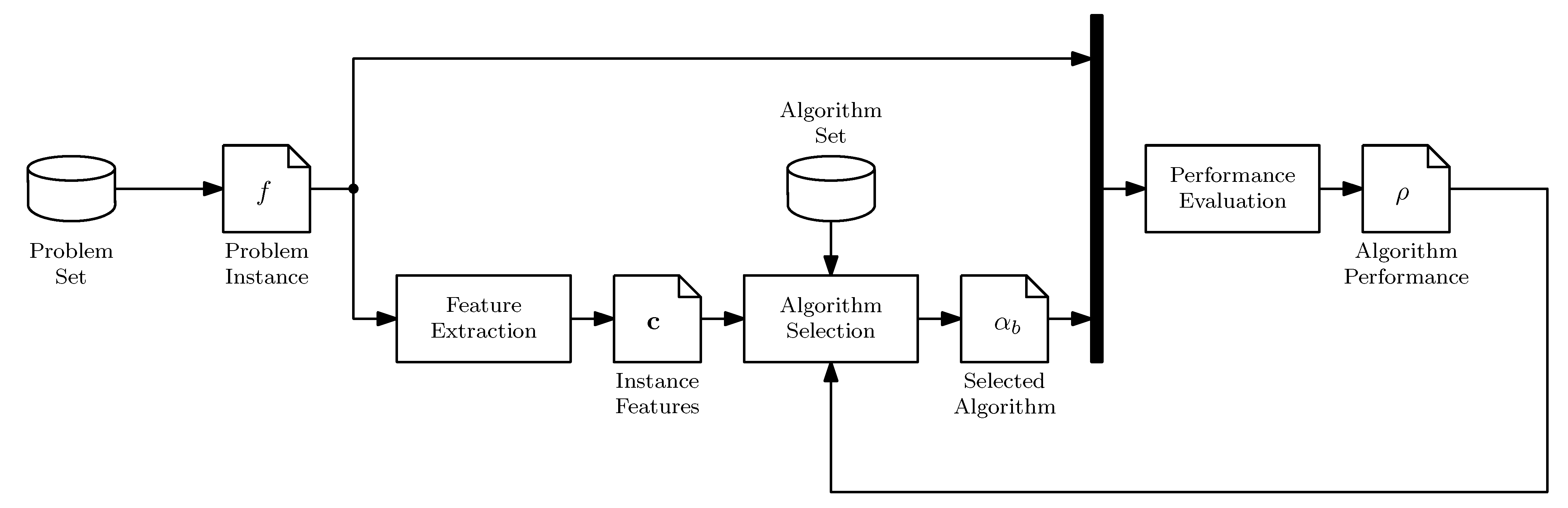
Rice [20] proposed an algorithm selection framework based on measurements of the characteristics of the problem. Successful implementations of this framework can be found in graph coloring, program induction, satisfiability, among other problem domains [28,29,30,31]. Our interpretation of the framework results in the selector illustrated in Figure 1, whose components are:
- Problem set () contains all the relevant BBO problems. It is hard to formally define and has infinite cardinality.
- Algorithm set () contains all search algorithms. This set potentially has infinite cardinality.
- Performance evaluation is a procedure to evaluate the solution quality or speed of a search algorithm in a function f, using a performance measure, .
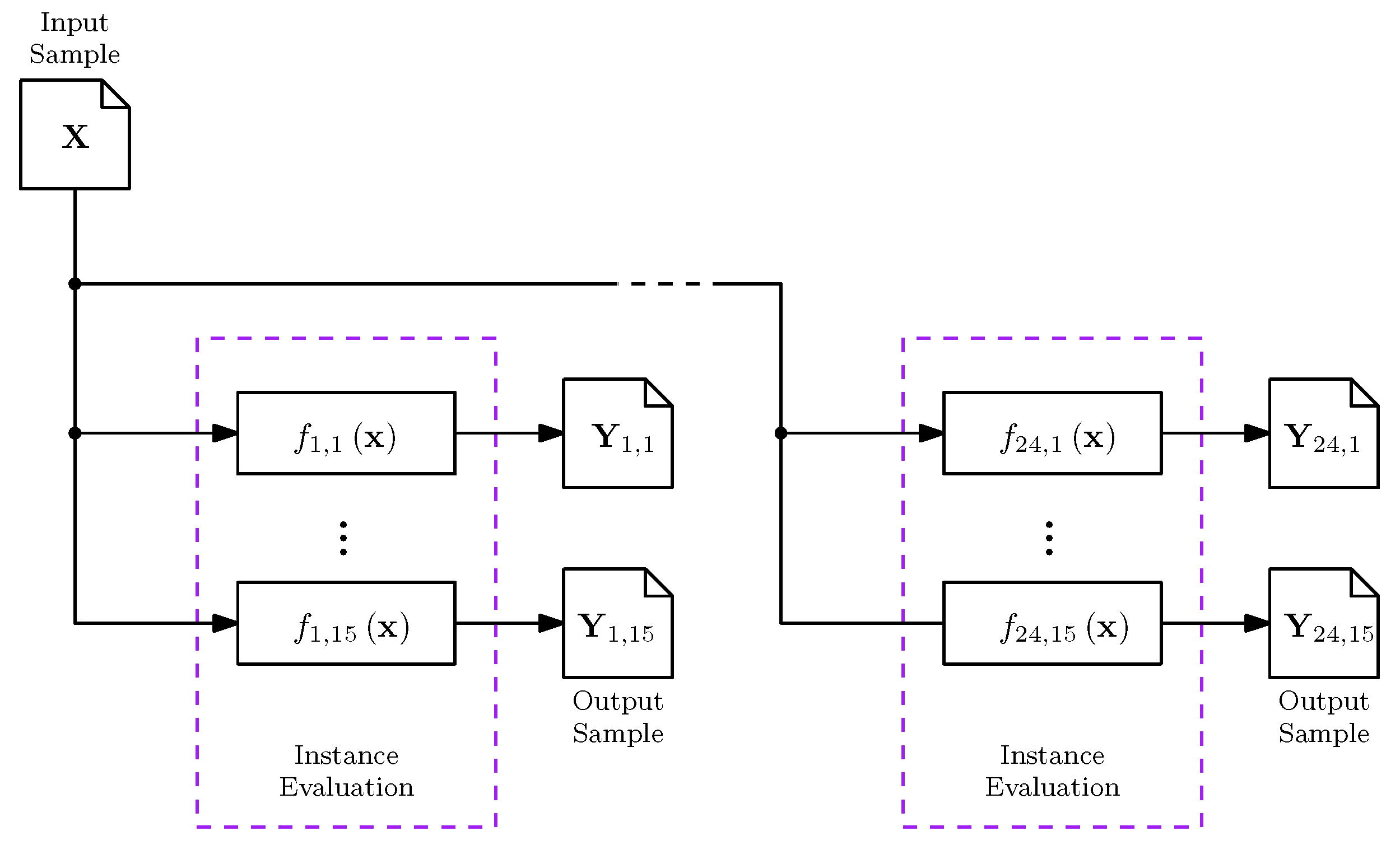
- Feature extraction is a procedure where an input sample, , is evaluated in the problem instance, resulting in an output sample, . These two samples are then used to calculate the ELA features, , as illustrated in Figure 2.
- Algorithm selection is a procedure to find the best algorithm using . Its main component is the learning model [28], as illustrated in Figure 2. The learning model maps the characteristics to the performance of a subset of complementary or well-established algorithms, , also known as algorithm portfolio. A method known as pre-selector constructs . The learning model is trained using experimental data contained in the knowledge base [32]. To predict the best performing algorithm for a new problem, it is necessary to estimate and evaluate the model.
3. Methods
In this section, we describe the architecture of the selector. Section 3.1 describes the structure of the learning model. Section 3.2 describes the details of the ELA features used as inputs. Section 3.3 describes the expected running time [33], which is used measure of algorithm performance.
3.1. Learning Model
We use as learning model a multi-class classification model, in which each class represents the best performing algorithm, instead of a regression model, which predicts the actual performance of the algorithms. Classification avoids the censoring issue existing in regression, i.e., one or more algorithms cannot find a target solution for all the problems in the training set, leaving gaps on the knowledge base. Although these gaps may be ignored or corrected, it is still possible for a regression model to overestimate the performance [30]. On the other hand, a classification model will be properly fitted if there is at least one algorithm that finds the target solution.
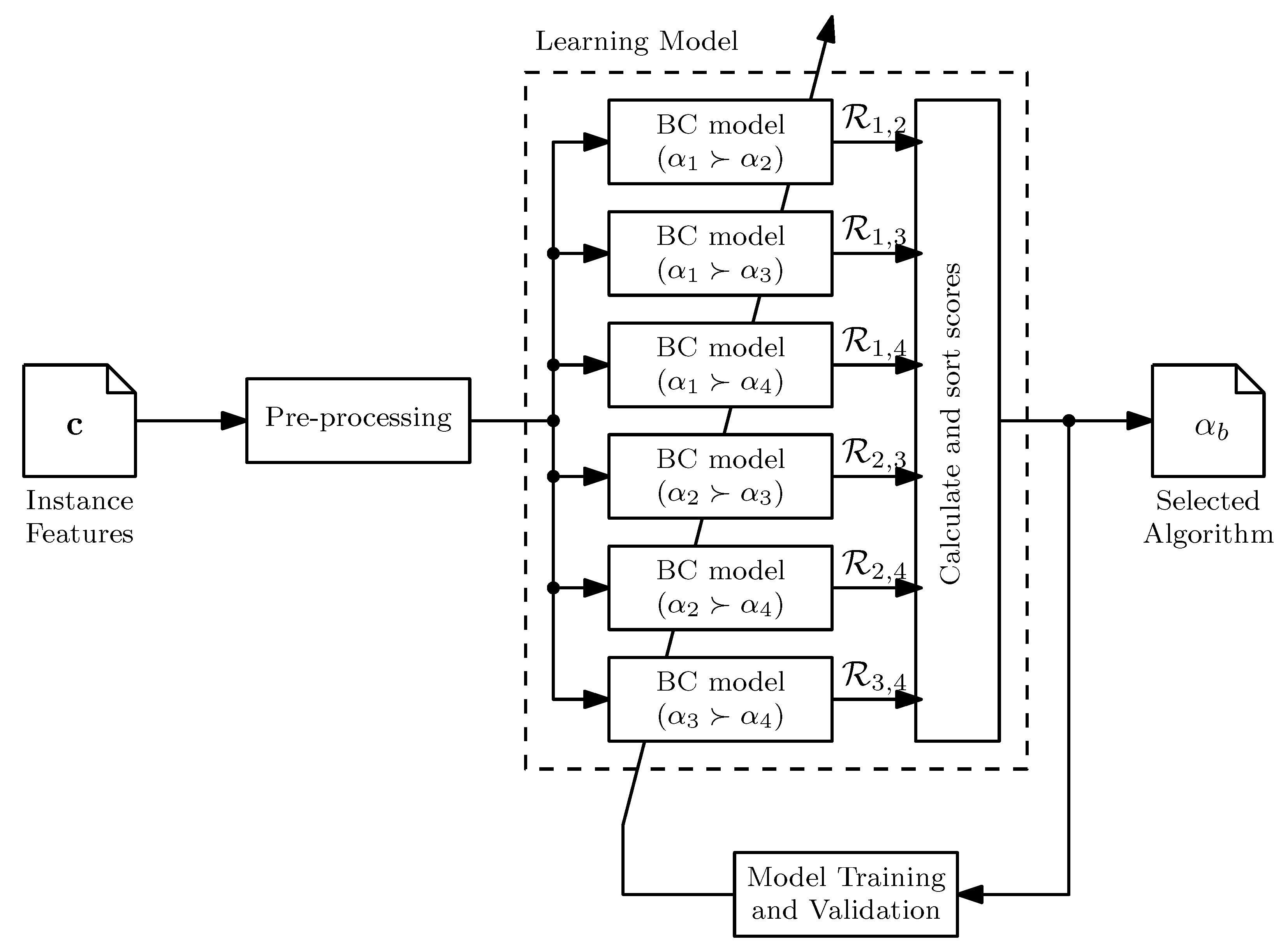
An ensemble of Binary Classification (BC) models is used where each one produces a probability score, , as output, where are candidate algorithms in a set . This score represents the truth level of . Correspondingly, . The pairwise scores are combined to generate an algorithm score, . The selected algorithm is the one that maximizes [34]. The architecture of the model is illustrated in Figure 3 for a portfolio of four algorithms. This architecture does have some shortcomings worth acknowledgment. The number of individual BC models increases at . However, as shown by Bischl et al. [35], only a small number of algorithms are required to obtain good performance in many domains. Moreover, it is possible for the model to select the worst performing algorithm due to a classification error. This results in performance degradation on problems for which all the algorithms find target solutions, or no solution at all, or if only one algorithm finds a target solution.
3.2. Exploratory Landscape Analysis Features
As inputs to the selector, we use the features summarized in Table 1, as they are quick and simple to calculate. Furthermore, these features can share a sample obtained through a Latin Hypercube Design (LHD), guaranteeing that the differences observed between features depend only on the instance, and not on sample size or sampling method. For example, the convexity and local search methods described by [8] use independent sampling approaches; hence, they cannot share a sample between them nor with the methods in Table 1. The convexity method takes two candidates, , and forms a linear combination with random weights, . Then, the difference between and the convex combination of and is computed. The result is the number of iterations out of 1000 in which the difference is less than a threshold. Meanwhile, the local search method uses the Nelder–Mead algorithm, starting from 50 random points. The solutions are hierarchically clustered to identify the local optima of the function. The basin of attraction of a local optimum, , i.e., the subset from from which a local search converges to , is approximated by the number of algorithm runs that terminate at each . Both sampling approaches do not guarantee the resulting sample is unbiased; hence, reusable. Besides ensuring a fair comparison, sharing a LHD sample reduces the overall computational cost, as no new candidates must be taken from the space.
The adjusted coefficient of determination, , measures the fit of linear or quadratic least squares regression models. This approach estimates the level of modality and the global structure [8], and it can be thought of as measuring the distance between a problem under analysis and a reference one [29]. To provide information about variable scaling, the ratio between the minimum and the maximum absolute values of the quadratic term coefficients in the quadratic model, , is also calculated [8].
The mutual information can be used as a measure of non-linear variable dependency [36]. Let be a set of variables indexes, and be a combination of such variables. The information significance, , is calculated as follows:
where is the information entropy, is the mutual information, with being the cost of . The information entropy of a continuous distribution is estimated through a -tree partition method [37] and it is not bounded between . Let be the order of information significance. The mean information significance of order k is defined as:
Please note that as D increases the number of possible variable combinations increases. Therefore, we limit ourselves to .
The probability distribution of may indicate whether the function is neutral, smooth or rugged, as well as the existence or lack of a global structure [8]. The shape of the distribution is characterized by estimating the sample skewness, , and kurtosis, [8], and entropy, [38].
Other reported measures with similar sampling simplicity were discarded as they are co-linear with those in Table 1 [16]. For example: Fitness distance correlation [39], , is co-linear with (). Dispersion at 1%, , is co-linear with D (). The adjusted coefficient of determination of a linear regression model, , is co-linear with (). The adjusted coefficient of determination of a quadratic regression model including variable interactions, , is co-linear with (). The minimum of the absolute value of the linear model coefficients [8], , is co-linear with (). The maximum of the absolute value of the linear model coefficients, , is co-linear with (). Significance of second order [36], , is co-linear with (). Finally, the length scale entropy [40], , is co-linear with ().
3.3. Algorithm Performance Measure
To measure the efficiency of an algorithm—and indirectly the selector—we use the expected running time, , which estimates the average number of function evaluations required by an algorithm to reach within a target precision for the first time [33]. A normalized, log-transformed version is calculated as follows:
where is the target precision, is the number of function evaluations over all runs where the best cost, , is greater than the optimal cost, and is the number of successful runs. The distribution is log-transformed to compensate for its heavy left tail, i.e., most problems require many function evaluations to reach the target. When some runs are unsuccessful, depends on the termination criteria of the algorithm. The average expected running time over a subset of problems, , is defined as:
4. Selector Implementation
To implement the selector, our first step is to choose representative subsets for the problem, , and algorithm, , spaces. We use the MATLAB implementation of the Comparing Continuous Optimizers (COCO) noiseless benchmarks v13.09 [33] as representative of . The motivation for this choice of benchmark problems revolves around practical advantages. For example, there is a wealth of data collected about the performance of a large set of search algorithms, and there are established conventions on the number of dimensions and the limits on the function evaluation budget. The software implementation of COCO generates instances by translating and rotating the function in the input and output spaces. For example, let be a functions in COCO, where is an orthogonal rotation matrix, and cause translational shifts on the input and output space respectively. A function instance is generated by providing values for , , and . To allow replicable experiments, the software uniquely identifies each instance using an index. For each function at each dimension, we analyze instances at , giving us a total of 1440 problem instances for analysis.
As a representative subset of the algorithm space, , we have used a subset of algorithms from the Black-Box Optimization Benchmarking (BBOB) sessions, composed of CMA-ES, BIPOP-CMA-ES, LStep and Nelder–Mead with Resize and Half-Runs. Corresponding results are publicly available at the benchmark website (http://coco.gforge.inria.fr/doku.php). The subset was selected using ICARUS (Identification of Complementary algoRithms by Uncovered Sets), a heuristic method to construct portfolios based on uncovered sets, a concept derived from voting systems theory [41]. As a comparison algorithm we use a portfolio composed of the BFGS, BIPOP-CMA-ES, LSfminbnd, and LSstep algorithms (BBLL) [2]. In contrast to our automatically selected portfolios, the algorithms in this portfolio were manually selected to minimize over all the benchmark functions within a target of . The descriptions of all algorithms employed are presented in Table 2.
As our next step, we calculate the ELA features. Ideally, if the features are to be used for algorithm selection, their additional computational cost should be a fraction of the cost associated with a single search algorithm, which is usually bounded at function evaluations [33]. Belkhir et al. [47] and Kerschke et al. [15] use sample sizes of and respectively, which are close to the population size of an evolutionary algorithm. However, Belkhir et al. [47] establishes that produces poor approximations of the feature values, although they can be improved by training and resampling a surrogate model. Nevertheless, their experiments also demonstrate that most features for the COCO benchmark set level-off between and . These results are supported by Škvorc et al. [13], who determined that for a sample size of at least was necessary to guarantee convergence.
Given this evidence, and to balance the cost of our computations, we set the lower bound for the sample size at , corresponding to 1% of the budget, and the upper bound at , corresponding to 10% of the budget, which we consider to be reasonable sample sizes. We divided the range between and into five equally sized intervals in base-10 logarithmic scale, aiming to produce a geometric progression analogous to the progression in D. As a result, we have five samples for each dimension. The samples have sizes n equal to points, where each one is roughly 80% larger than the previous. We generate the input samples, , using MATLAB’s Latin Hypercube Sampling function lhsdesign with default parameters.
We generate the output sample, , by evaluating in one of the first 15 instances of the 24 functions from COCO, guaranteeing that the differences observed on the ELA features only depend on the function value and sample size, as illustrated in Figure 4. As D increases, the size of becomes relatively smaller because the input space has increased geometrically, while the sample has increased linearly. This is an unavoidable limitation due to the curse of dimensionality. The combination of input/output sample are analyzed using the features. To sum up, the input patterns database for a sample size n has a total of 1440 observations, one per each instance, with ten predictors. All data used for training is made available in the LEarning and OPtimization Archive of Research Data (LEOPARD) v1.0 [19].
5. Selector Validation
Given the data-driven nature of the ELA features, the randomness and size of the input sample used to calculate may also affect accuracy. Therefore, through the validation process we aim to answer the following questions:
- Q1
- Does the selector’s accuracy increases with the size of the sample used to calculate the ELA features?
- Q2
- What is the effect of the sample randomness on the selector performance?
The validation process is based on the Hold-One-Instance-Out (HOIO) and Hold-One-Problem-Out (HOPO) approaches proposed by Bischl et al. [2]. For HOIO, the data from one instance of each problem at all dimensions is removed from the training set. For HOPO, all the instances for one problem at all dimensions are removed from the training set. HOIO measures the performance for instances of problems previously observed; whereas HOPO measures the performance for instances of unobserved problems.
To answer Q1, we train 30 different models for each validation approach, and average the performance over them. We use a cost-sensitive Random Forest (RF) classification model with 100 binary trees, which weighted each observation according to the difference in performance between algorithms [48] as BCs. The performance is measured for each value of n in terms of the success, best and worst-case selection, and total failure rates. The Success Rate () is the percentage of solved problems by the selector; the Best Case Selection Rate () is the percentage of problems for which the best algorithm was selected; the Worst-Case Selection Rate () is the percentage of problems for which the worst algorithm was selected; and the Total Failure Rate () is the percentage of unsolved problems due to selecting the worst performing algorithm. To summarize the efficiency and accuracy results of the selector, we define a normalized performance score, , as follows:
where is a baseline algorithm for which . For our cases, the baseline algorithm will be the BBLL portfolio with random selection, .
Once we have verified that the architecture of the selector produces satisfactory results, we address Q2. To do this, we estimate the empirical probability distribution of each feature, . There are multiple approaches to this problem. For example, to take multiple, independent trial sets per function [17], which guarantees the most accurate estimator of , although with the substantial computational of cost collecting the function responses and calculating the features, particularly as n and D increase. Another approach is to train a surrogate model with a small sample, and then resample from the model [47], which provides a low computational cost estimate of , although the resample also includes assumptions generated by the surrogate which may not correspond to the actual function. Moreover, parametric assumptions cannot be made, and there is no guarantee of fulfilling asymptotic convergence. Therefore, we use bootstrapping [49] to estimate , which allows us to use one, potentially small sample, hence it can be applied on expensive problems, without adding assumptions to the methodology.
Bootstrapping is a type of resampling method that uses the empirical distribution to learn about the population distribution as follows: Let be a sample of n independent and identically distributed random variables drawn from the distribution . We can consider to be a summary statistic of , for example the mean, the standard deviation, or in our case an ELA feature. Let be a bootstrap sample, which is a new set of n points independently sampled with replacement from . From each one of the N bootstrap samples, we calculate a bootstrap statistic, , also in our case a feature. In other words, from each sample of size n we create N resamples with replacement, also of size n, from which we estimate all the features. This feature vectors are fed into the meta-models during the HOIO and HOPO validation. With , we estimate the 95% confidence intervals and bias of for all values of n. The confidence intervals are estimated using Efron’s non-parametric corrected percentile method [50], i.e., we compute the 2.5th and 97.5th percentiles of the bootstrap distributions for each performance measure.
6. Results
6.1. Performance of the Selector
We now provide an answer to the questions formulated above. The results show that a larger value of n does not translate to higher selection accuracy, while greatly increasing the cost for easier problems. The remaining budget to find a solution decreases due to an increase of used to estimate the ELA features. Furthermore, changes in the input sample have minor effects on the performance. This implies that the selector is reliable even with noisy features, suggesting that their variance is small. Let us examine the results in detail.
The performance of the best algorithm for a given problem is illustrated in Figure 5 for the ICARUS/HOPO and BBLL portfolios. We observe that BIPOP-CMA-ES is the dominant algorithm for dimensions in both portfolios. The Nelder–Doerr algorithm replaces BFGS in the ICARUS/HOPO portfolio, resulting in deterioration of for . There are specialized algorithms for particular problems regardless of the number of dimensions, e.g., LSstep is the best for . Table 3 shows the performance of the individual algorithms, the selectors during HOIO and HOPO. In addition, the results from an oracle, i.e., a method which always selects the best algorithm without incurring any cost, and a random selector are presented. The performance is measured as , the 95% Confidence Interval (CI) of , , , , , and . In boldface are the best values of each performance measure over each validation method and . The table shows that only the oracles achieve , with the ICARUS portfolio having the best overall performance with during HOPO. The table also shows that is always the lowest for , given that less of the budget is used to calculate the ELA features. Highest is achieved with for the ICARUS portfolios and for the BBLL portfolio. However, the differences with smaller n may not justify the additional cost. For example, a of and a of is achieved with for the ICARUS sets, a difference of in and in for . Compared with total random selection, the selectors’ and are at least one order of magnitude smaller. Table 3 also shows on average a decrease on of , an increase of and of ≈7% and ≈3% respectively; although the results for the ICARUS sets are below average for and , indicating better performance. Furthermore, is always above 90% for the ICARUS sets, while falls below 90% during HOPO for the BBLL set. Only BIPOP-CMA-ES with can match the overall performance of a selector.
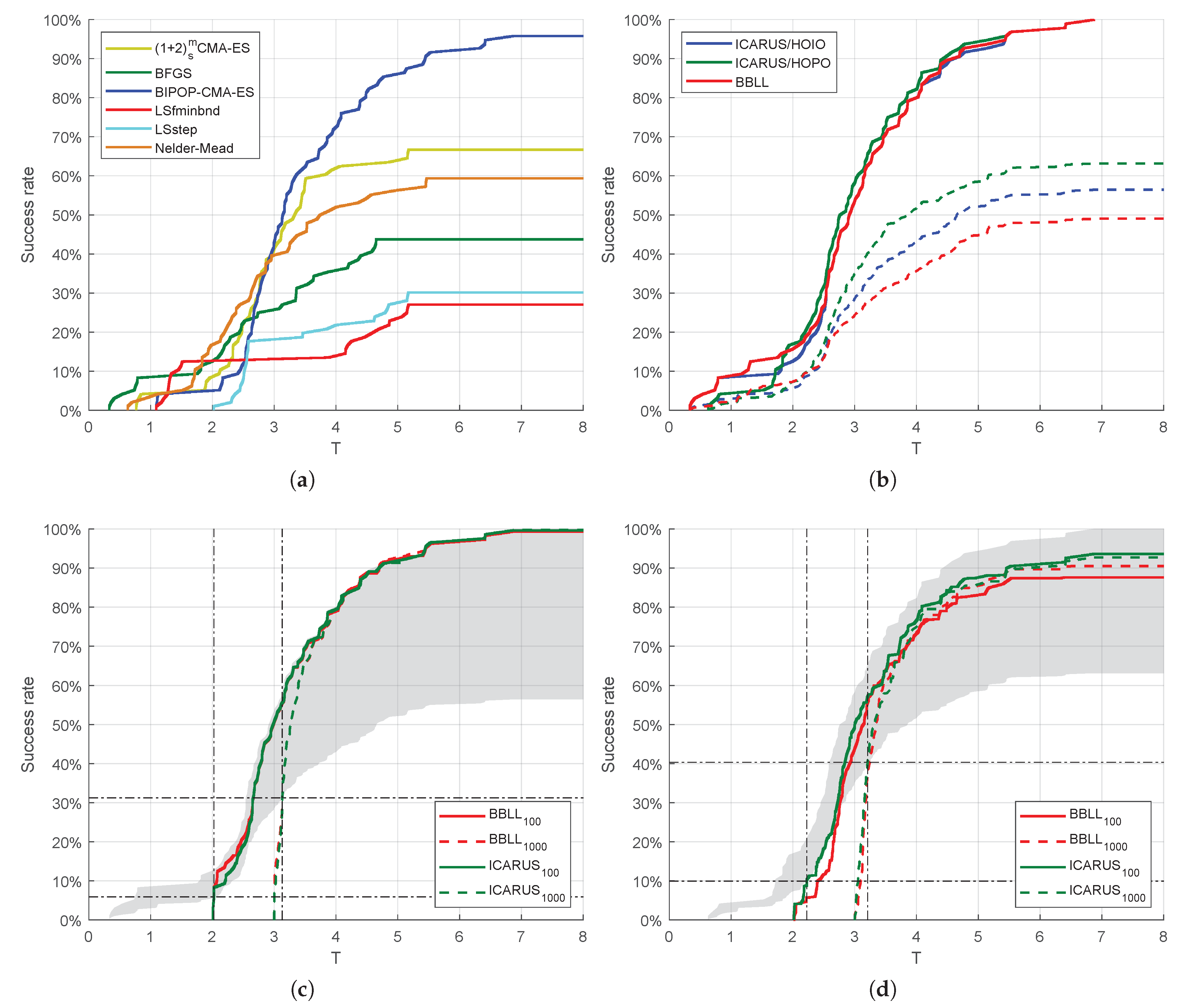
Figure 6 illustrate the against for the complete benchmark set. Figure 6a shows the results of individual algorithms, while Figure 6b shows the performance of such oracle as solid lines and the random selector as dashed lines for the ICARUS/HOIO, ICARUS/HOPO, and BBLL portfolios. As expected from Figure 5a, the ICARUS/HOPO oracle has a degradation in performance in the easier 10% of the problems. On the top 10% of the problems the performance of the three oracles is equivalent. The ICARUS/HOPO oracle has a small improvement on performance between 10% and 90% of the problems. Figure 6c,d illustrate the performance of the selectors for . The shaded region indicates the theoretical area of performance, with the upper bound representing the ICARUS oracle and the lower bound random selection. Although it is unfeasible to match the performance of the oracle, due to the cost of extracting the ELA measures and a less than 100%, the figure shows the performance improvement against random selection. During HOIO, the ICARUS selector surpasses random selection at with , representing 5.9% of the problems; and at with , representing 31.2% of the problems. During HOPO, the ICARUS selector surpasses random selection at with , representing 9.9% of the problems; and at with , representing 40.3% of the problems.
To understand where the selectors fail, we calculate the average , , and for a given problem or a given dimension during HOIO and HOPO validations. Table 4 shows these results, where in boldface are the and less than 90%, and the and higher than 10%. The table shows that an instance of either have the highest possibility of remaining unsolved, despite the model having information about other instances of these functions. Some problems, such as , have high and low values, which can be explained by their simplicity, as most algorithms can solve them. The performance appears to be evenly distributed in terms of dimension. Overall, the selector appears to struggle with those problems where only one algorithm may be the best. Nevertheless, these results indicate that the architecture of the selector is adequate for testing the effect of systemic errors.
6.2. Sampling Effects on Selection
Table 5 shows the 95% CI of . The sub-index represents estimation bias, defined as the difference between the bootstrap mean and the original mean, which was presented in Table 3. A large bias implies that the estimated CI is less reliable. In boldface are those intervals whose range is the smallest for a given validation. The lowest bias is also in boldface. This table shows the smallest range is achieved with , implying more stable predictions are made the selector with a large sample size. This also implies more stable ELA features. However, the differences are relatively minor. For example, the difference between the upper and lower bounds of represent 65 for , 63 for , and 37 for . For , the difference is 0.8% for , 0.6% for , and 0.4% for . Hence, the ELA features are sufficiently stable with a small n, to achieve reliable selection by the selector.
7. Discussion
The overarching aim of this paper was to explore the effect that uncertainty in the features has on the performance of automated algorithm selectors. To meet this aim, we have designed, implemented and validated an algorithm selector, and analyzed the effects that the features accuracy have on the selector performance. These methods were described in Section 3. We have carried out an experimental validation using the COCO noiseless benchmark set [33] as representative problems. The results described in Section 6 are encouraging, as they demonstrate that as long as the features are informative, and have low variability, the selection error will be small. This conclusion is the main contribution of our paper. However, there are several trade-offs in the selector performance associated with the methodology employed. We discuss these points in detail below.
The results have shown that an increase in the sample size n does not improve and . On the contrary, large sample sizes deteriorate the performance in terms of for the easier problems. Although is a reasonable cost for calculating the ELA features, this cost could be distributed if each candidate used to calculate features is also the starting point of a random restart. It is known that random restarts improve the heavy-tailed behavior of optimization algorithms [51]. It may also be possible that an optimal n exists for every problem instance and ELA measure. Potentially, n could be decreased until the accuracy of the selector deteriorates. However, it should be noted that the learning model does not predict the variance of , which is an indicator of the reliability of the algorithm. Therefore, the selector does not differentiate between reliable and unreliable algorithms. A model that predicts the variance may improve the selector accuracy. Further investigation of these issues is left for further research.
The results confirm that the ‘no-free-lunch’ theorem [27] still holds for the selector. The cost of ELA stage decreases the selector performance in the simplest problems compared to a method such as BFGS. Moreover, a parallel implementation of the portfolio would certainly achieve a with a trade-off on . However, it should be noted that the component algorithms were selected using the complete information from the knowledge base. Hence, it is an estimate of the ideal performance. A key advantage of the selector is that after the allocated budget exceeds a threshold, performance gains are evident, particularly if the budget is a few orders of magnitude larger. Therefore, the selector is competitive when the precision of the solution is more important than the computational cost. Considering a BBO problem, where there is no certainty about the difficulty, the selector gives some assurances that a solution could be found with a small trade-off. Additionally, the results show that the selector is robust to noise in the ELA features.
Due to their algorithmic simplicity and scalability with D, the ELA features allowed us to ‘sample once and measure many’. Therefore, they reduced the cost measured as of the measuring phase. However, this does not mean that they are sufficient, complete or even necessary. Therefore, other features may be investigated that may potentially improve accuracy.
Finally, the reduced number of problems in the COCO benchmark set limits the generality of our results. The set is considered to be a space filling benchmark set [2]. However, this conclusion was based on a graphical representation, which is dependent on the employed ELA features. Therefore, we consider it necessary to add functions to the training set. This can be accomplished by using an automatic generator [52] or examining other existing benchmark sets. In conjunction with a visualization technique, this approach may reveal new details about the nature of the problem set [31]. This is a significant challenge in continuous BBO, for which the selector is a fundamental part of the solution.
Author Contributions
Conceptualization, M.A.M. and M.K.; methodology, M.A.M.; software, M.A.M.; validation, M.A.M; formal analysis, M.A.M.; data curation, M.A.M.; writing—original draft preparation, M.A.M.; writing—review and editing, M.K.; supervision, M.K.; funding acquisition, M.A.M. All authors have read and agreed to the published version of the manuscript.
Funding
This work was funded by The University of Melbourne through MIRS/MIFRS scholarships awarded to M.A. Muñoz.
Data Availability Statement
The data presented in this study are openly available in FigShare at DOI:10.6084/m9.figshare.c.5106758.
Acknowledgments
We thank Saman Halgamuge and Kate Smith-Miles for the support in the preparation of this manuscript.
Conflicts of Interest
The authors declare no conflict of interest. The funders had no role in the design of the study; in the collection, analyses, or interpretation of data; in the writing of the manuscript, or in the decision to publish the results.
References
- Lozano, M.; Molina, D.; Herrera, F. Editorial scalability of evolutionary algorithms and other metaheuristics for large-scale continuous optimization problems. Soft Comput. 2011, 15, 2085–2087. [Google Scholar] [CrossRef]
- Bischl, B.; Mersmann, O.; Trautmann, H.; Preuß, M. Algorithm selection based on exploratory landscape analysis and cost-sensitive learning. In Proceedings of the 14th Annual Conference on Genetic and Evolutionary Computation (GECCO’12), Philadelphia, PA, USA, 7–11 July 2012; pp. 313–320. [Google Scholar] [CrossRef]
- Muñoz, M.; Kirley, M.; Halgamuge, S. A Meta-Learning Prediction Model of Algorithm Performance for Continuous Optimization Problems. In Proceedings of the International Conference on Parallel Problem Solving from Nature, PPSN XII, Taormina, Italy, 1–5 September 2012; Volume 7941, pp. 226–235. [Google Scholar] [CrossRef]
- Abell, T.; Malitsky, Y.; Tierney, K. Features for Exploiting Black-Box Optimization Problem Structure. In LION 2013: Learning and Intelligent Optimization; LNCS; Springer: Berlin/Heidelberg, Germany, 2013; Volume 7997, pp. 30–36. [Google Scholar]
- Belkhir, N.; Dréo, J.; Savéant, P.; Schoenauer, M. Feature Based Algorithm Configuration: A Case Study with Differential Evolution. In Parallel Problem Solving from Nature—PPSN XIV; Springer International Publishing: Berlin/Heidelberg, Germany, 2016; pp. 156–166. [Google Scholar] [CrossRef] [Green Version]
- Belkhir, N.; Dréo, J.; Savéant, P.; Schoenauer, M. Per instance algorithm configuration of CMA-ES with limited budget. In Proceedings of the Genetic and Evolutionary Computation Conference, Berlin, Germany, 15–19 July 2017. [Google Scholar] [CrossRef] [Green Version]
- Kerschke, P.; Trautmann, H. Automated Algorithm Selection on Continuous Black-Box Problems by Combining Exploratory Landscape Analysis and Machine Learning. Evol. Comput. 2019, 27, 99–127. [Google Scholar] [CrossRef] [PubMed] [Green Version]
- Mersmann, O.; Bischl, B.; Trautmann, H.; Preuß, M.; Weihs, C.; Rudolph, G. Exploratory landscape analysis. In Proceedings of the 13th Annual Conference on Genetic and Evolutionary Computation, (GECCO’11), Dublin, Ireland, 12–16 July 2011; pp. 829–836. [Google Scholar] [CrossRef]
- Jansen, T. On Classifications of Fitness Functions; Technical Report CI-76/99; University of Dortmund: Dortmund, Germany, 1999. [Google Scholar]
- Müller, C.; Sbalzarini, I. Global Characterization of the CEC 2005 Fitness Landscapes Using Fitness-Distance Analysis. In Applications of Evolutionary Computation; LNCS; Springer: Berlin/Heidelberg, Germany, 2011; Volume 6624, pp. 294–303. [Google Scholar] [CrossRef] [Green Version]
- Tomassini, M.; Vanneschi, L.; Collard, P.; Clergue, M. A Study of Fitness Distance Correlation as a Difficulty Measure in Genetic Programming. Evol. Comput. 2005, 13, 213–239. [Google Scholar] [CrossRef]
- Saleem, S.; Gallagher, M.; Wood, I. Direct Feature Evaluation in Black-Box Optimization Using Problem Transformations. Evol. Comput. 2019, 27, 75–98. [Google Scholar] [CrossRef] [PubMed]
- Škvorc, U.; Eftimov, T.; Korošec, P. Understanding the problem space in single-objective numerical optimization using exploratory landscape analysis. Appl. Soft Comput. 2020, 90, 106138. [Google Scholar] [CrossRef]
- Muñoz, M.; Kirley, M.; Smith-Miles, K. Analyzing randomness effects on the reliability of Landscape Analysis. Nat. Comput. 2020. [Google Scholar] [CrossRef]
- Kerschke, P.; Preuß, M.; Wessing, S.; Trautmann, H. Low-Budget Exploratory Landscape Analysis on Multiple Peaks Models. In Proceedings of the Genetic and Evolutionary Computation Conference (GECCO ’16), Denver, CO, USA, 20–24 July 2016; ACM: New York, NY, USA, 2016; pp. 229–236. [Google Scholar] [CrossRef]
- Muñoz, M.; Smith-Miles, K. Effects of function translation and dimensionality reduction on landscape analysis. In Proceedings of the 2015 IEEE Congress on Evolutionary Computation (CEC) (IEEE CEC’15), Sendai, Japan, 25–28 May 2015; pp. 1336–1342. [Google Scholar] [CrossRef]
- Renau, Q.; Dreo, J.; Doerr, C.; Doerr, B. Expressiveness and robustness of landscape features. In Proceedings of the Genetic and Evolutionary Computation Conference Companion, GECCO’19, Prague, Czech Republic, 13–17 July 2019; ACM Press: New York, NY, USA, 2019. [Google Scholar] [CrossRef]
- Renau, Q.; Doerr, C.; Dreo, J.; Doerr, B. Exploratory Landscape Analysis is Strongly Sensitive to the Sampling Strategy. In Parallel Problem Solving from Nature—PPSN XVI; Bäck, T., Preuss, M., Deutz, A., Wang, H., Doerr, C., Emmerich, M., Trautmann, H., Eds.; Springer International Publishing: Berlin/Heidelberg, Germany, 2020; pp. 139–153. [Google Scholar]
- Muñoz, M. LEOPARD: LEarning and OPtimization Archive of Research Data. Version 1.0. 2020. Available online: https://0-doi-org.brum.beds.ac.uk/10.6084/m9.figshare.c.5106758 (accessed on 8 November 2020).
- Rice, J. The Algorithm Selection Problem. In Advances in Computers; Elsevier: Amsterdam, The Netherlands, 1976; Volume 15, pp. 65–118. [Google Scholar] [CrossRef] [Green Version]
- Reeves, C. Fitness Landscapes. In Search Methodologies; Springer: Berlin/Heidelberg, Germany, 2005; pp. 587–610. [Google Scholar] [CrossRef]
- Pitzer, E.; Affenzeller, M. A Comprehensive Survey on Fitness Landscape Analysis. In Recent Advances in Intelligent Engineering Systems; SCI; Springer: Berlin/Heidelberg, Germany, 2012; Volume 378, pp. 161–191. [Google Scholar] [CrossRef]
- Weise, T.; Zapf, M.; Chiong, R.; Nebro, A. Why Is Optimization Difficult. In Nature-Inspired Algorithms for Optimisation; SCI; Springer: Berlin/Heidelberg, Germany, 2009; Volume 193, pp. 1–50. [Google Scholar] [CrossRef]
- Mersmann, O.; Preuß, M.; Trautmann, H. Benchmarking Evolutionary Algorithms: Towards Exploratory Landscape Analysis. In PPSN XI; LNCS; Springer: Berlin/Heidelberg, Germany, 2010; Volume 6238, pp. 73–82. [Google Scholar] [CrossRef] [Green Version]
- García-Martínez, C.; Rodriguez, F.; Lozano, M. Arbitrary function optimisation with metaheuristics. Soft Comput. 2012, 16, 2115–2133. [Google Scholar] [CrossRef]
- Hutter, F.; Hamadi, Y.; Hoos, H.; Leyton-Brown, K. Performance prediction and automated tuning of randomized and parametric algorithms. In CP ’06: Principles and Practice of Constraint Programming—CP 2006; LNCS; Springer: Berlin/Heidelberg, Germany, 2006; Volume 4204, pp. 213–228. [Google Scholar] [CrossRef] [Green Version]
- Wolpert, D.; Macready, W. No free lunch theorems for optimization. IEEE Trans. Evol. Comput. 1997, 1, 67–82. [Google Scholar] [CrossRef] [Green Version]
- Smith-Miles, K. Cross-disciplinary perspectives on meta-learning for algorithm selection. ACM Comput. Surv. 2009, 41, 6:1–6:25. [Google Scholar] [CrossRef]
- Graff, M.; Poli, R. Practical performance models of algorithms in evolutionary program induction and other domains. Artif. Intell. 2010, 174, 1254–1276. [Google Scholar] [CrossRef]
- Hutter, F.; Xu, L.; Hoos, H.; Leyton-Brown, K. Algorithm runtime prediction: Methods & evaluation. Artif. Intell. 2014, 206, 79–111. [Google Scholar] [CrossRef]
- Smith-Miles, K.; Baatar, D.; Wreford, B.; Lewis, R. Towards objective measures of algorithm performance across instance space. Comput. Oper. Res. 2014, 45, 12–24. [Google Scholar] [CrossRef]
- Hilario, M.; Kalousis, A.; Nguyen, P.; Woznica, A. A data mining ontology for algorithm selection and meta-mining. In Proceedings of the Second Workshop on Third Generation Data Mining: Towards Service-Oriented Knowledge Discovery (SoKD’09), Bled, Slovenia, 7 September 2009; pp. 76–87. [Google Scholar]
- Hansen, N.; Auger, A.; Finck, S.; Ros, R. Real-Parameter Black-Box Optimization Benchmarking BBOB-2010: Experimental Setup; Technical Report RR-7215; INRIA Saclay-Île-de-France: Paris, France, 2014. [Google Scholar]
- Hüllermeier, E.; Fürnkranz, J.; Cheng, W.; Brinker, K. Label ranking by learning pairwise differences. Artif. Intell. 2008, 172, 1897–1916. [Google Scholar] [CrossRef] [Green Version]
- Bischl, B.; Kerschke, P.; Kotthoff, L.; Lindauer, M.; Malitsky, Y.; Fréchette, A.; Hoos, H.; Hutter, F.; Leyton-Brown, K.; Tierney, K.; et al. ASlib: A benchmark library for algorithm selection. Artif. Intell. 2016, 237, 41–58. [Google Scholar] [CrossRef] [Green Version]
- Seo, D.; Moon, B. An Information-Theoretic Analysis on the Interactions of Variables in Combinatorial Optimization Problems. Evol. Comput. 2007, 15, 169–198. [Google Scholar] [CrossRef]
- Stowell, D.; Plumbley, M. Fast Multidimensional Entropy Estimation by k-d Partitioning. IEEE Signal Process. Lett. 2009, 16, 537–540. [Google Scholar] [CrossRef]
- Marin, J. How landscape ruggedness influences the performance of real-coded algorithms: A comparative study. Soft Comput. 2012, 16, 683–698. [Google Scholar] [CrossRef]
- Jones, T.; Forrest, S. Fitness Distance Correlation as a Measure of Problem Difficulty for Genetic Algorithms. In Proceedings of the Sixth International Conference on Genetic Algorithms, Pittsburgh, PA, USA, 15–19 July 1995; Morgan Kaufmann Publishers Inc.: Burlington, MA, USA, 1995; pp. 184–192. [Google Scholar]
- Morgan, R.; Gallagher, M. Length Scale for Characterising Continuous Optimization Problems. In PPSN XII; LNCS; Springer: Berlin/Heidelberg, Germany, 2012; Volume 7941, pp. 407–416. [Google Scholar]
- Muñoz, M.; Kirley, M. ICARUS: Identification of Complementary algoRithms by Uncovered Sets. In Proceedings of the 2016 IEEE Congress on Evolutionary Computation (CEC) (IEEE CEC’16), Vancouver, BC, Canada, 24–29 July 2016; pp. 2427–2432. [Google Scholar] [CrossRef]
- Auger, A.; Brockhoff, D.; Hansen, N. Comparing the (1+1)-CMA-ES with a Mirrored (1+2)-CMA-ES with Sequential Selection on the Noiseless BBOB-2010 Testbed. In Proceedings of the 12th Annual Conference Companion on Genetic and Evolutionary Computation (GECCO’10), Portland, OR, USA, 7–11 July 2010; Association for Computing Machinery: New York, NY, USA, 2010; pp. 1543–1550. [Google Scholar] [CrossRef] [Green Version]
- Ros, R. Benchmarking the BFGS Algorithm on the BBOB-2009 Function Testbed. In GECCO’09: Proceedings of the 11th Annual Conference Companion on Genetic and Evolutionary Computation Conference: Late Breaking Papers; ACM: New York, NY, USA, 2009; pp. 2409–2414. [Google Scholar] [CrossRef] [Green Version]
- Hansen, N. Benchmarking a bi-population CMA-ES on the BBOB-2009 Function Testbed. In GECCO’09: Proceedings of the 11th Annual Conference Companion on Genetic and Evolutionary Computation Conference: Late Breaking Papers; ACM: New York, NY, USA, 2009; pp. 2389–2396. [Google Scholar] [CrossRef] [Green Version]
- Pošík, P.; Huyer, W. Restarted Local Search Algorithms for Continuous Black Box Optimization. Evol. Comput. 2012, 20, 575–607. [Google Scholar] [CrossRef] [Green Version]
- Doerr, B.; Fouz, M.; Schmidt, M.; Wahlstrom, M. BBOB: Nelder-Mead with Resize and Halfruns. In GECCO’09: Proceedings of the 11th Annual Conference Companion on Genetic and Evolutionary Computation Conference: Late Breaking Papers; ACM: New York, NY, USA, 2009; pp. 2239–2246. [Google Scholar] [CrossRef]
- Belkhir, N.; Dréo, J.; Savéant, P.; Schoenauer, M. Surrogate Assisted Feature Computation for Continuous Problems. In LION 2016: Learning and Intelligent Optimization; Lecture Notes in Computer Science; Springer International Publishing: Berlin/Heidelberg, Germany, 2016; pp. 17–31. [Google Scholar] [CrossRef] [Green Version]
- Xu, L.; Hutter, F.; Hoos, H.; Leyton-Brown, K. SATzilla: Portfolio-based algorithm selection for SAT. J. Artif. Intell. Res. 2008, 32, 565–606. [Google Scholar] [CrossRef] [Green Version]
- Efron, B.; Tibshirani, R. An Introduction to the Bootstrap; Chapman & Hall: London, UK, 1993. [Google Scholar]
- Efron, B. Nonparametric Standard Errors and Confidence Intervals. Can. J. Stat./ Rev. Can. Stat. 1981, 9, 139–158. [Google Scholar] [CrossRef]
- Gomes, C.; Selman, B.; Crato, N.; Kautz, H. Heavy-Tailed Phenomena in Satisfiability and Constraint Satisfaction Problems. J. Autom. Reason. 2000, 24, 67–100. [Google Scholar] [CrossRef]
- Smith-Miles, K.; van Hemert, J. Discovering the suitability of optimisation algorithms by learning from evolved instances. Ann. Math. Artif. Intel. 2011, 61, 87–104. [Google Scholar] [CrossRef]
Figure 1.
Diagram of the algorithm selector based on Rice’s framework [20]. The selector has three main components: Performance evaluation, Feature extraction, and Algorithm selection.
Figure 1.
Diagram of the algorithm selector based on Rice’s framework [20]. The selector has three main components: Performance evaluation, Feature extraction, and Algorithm selection.

Figure 2.
Details of the feature extraction and algorithm selection processes.
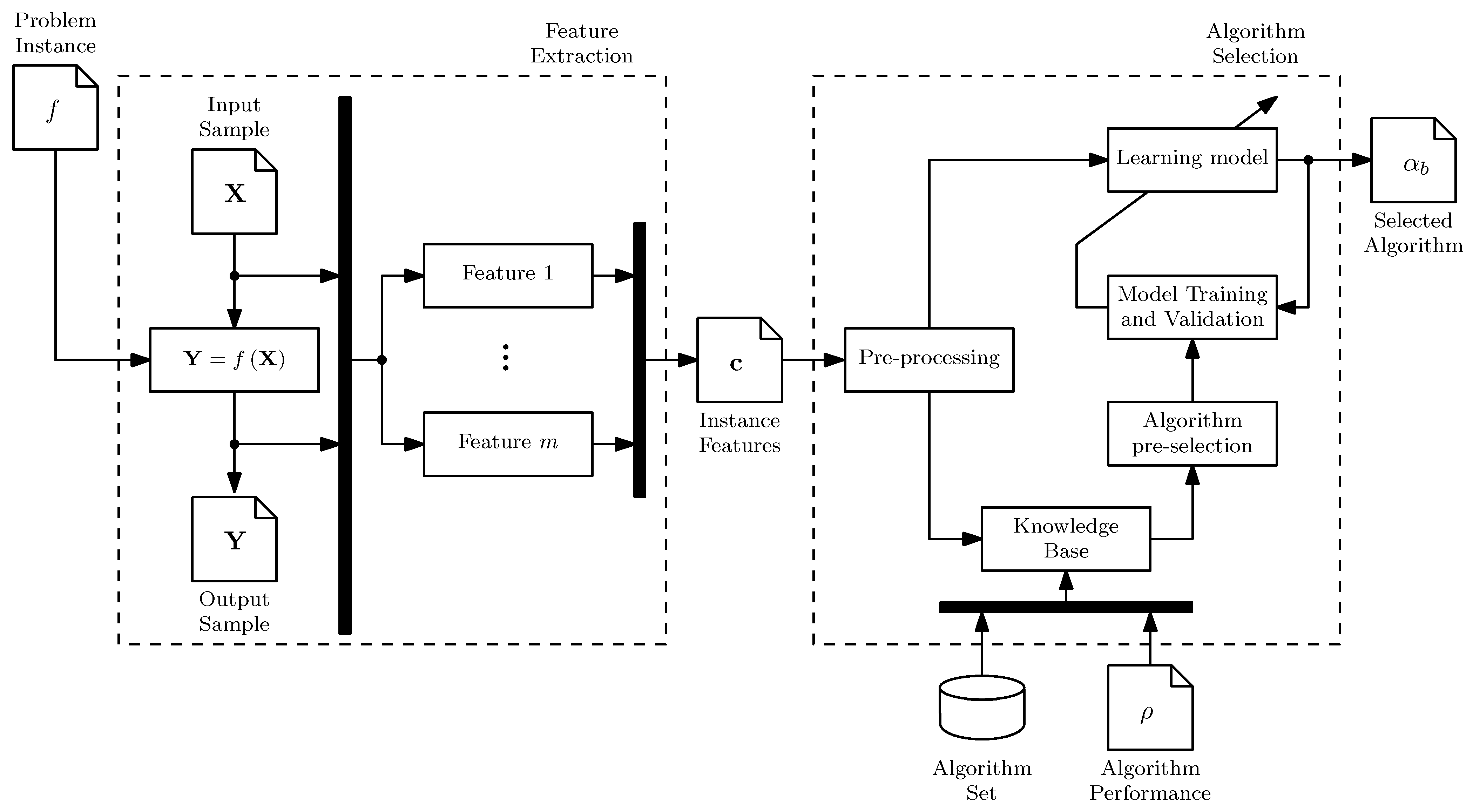
Figure 3.
Structure of the multi-class learning model for . The six BC models take the vector ELA features as input and generate a probability score, , which are used to generate a recommended algorithm as output.
Figure 3.
Structure of the multi-class learning model for . The six BC models take the vector ELA features as input and generate a probability score, , which are used to generate a recommended algorithm as output.

Figure 4.
Instance evaluation procedure. An input sample is evaluated in all the problem instances , where i is the function index, and j the instance index. The result is an output sample . The procedure guarantees that the differences among measures only depend on the output sample.
Figure 4.
Instance evaluation procedure. An input sample is evaluated in all the problem instances , where i is the function index, and j the instance index. The result is an output sample . The procedure guarantees that the differences among measures only depend on the output sample.

Figure 5.
Performance of the best algorithm in terms of for each problem. The lines represent the dimension of the problem. The Nelder–Doerr algorithm replaces BFGS in the ICARUS/HOPO portfolio in most of the problems.
Figure 5.
Performance of the best algorithm in terms of for each problem. The lines represent the dimension of the problem. The Nelder–Doerr algorithm replaces BFGS in the ICARUS/HOPO portfolio in most of the problems.
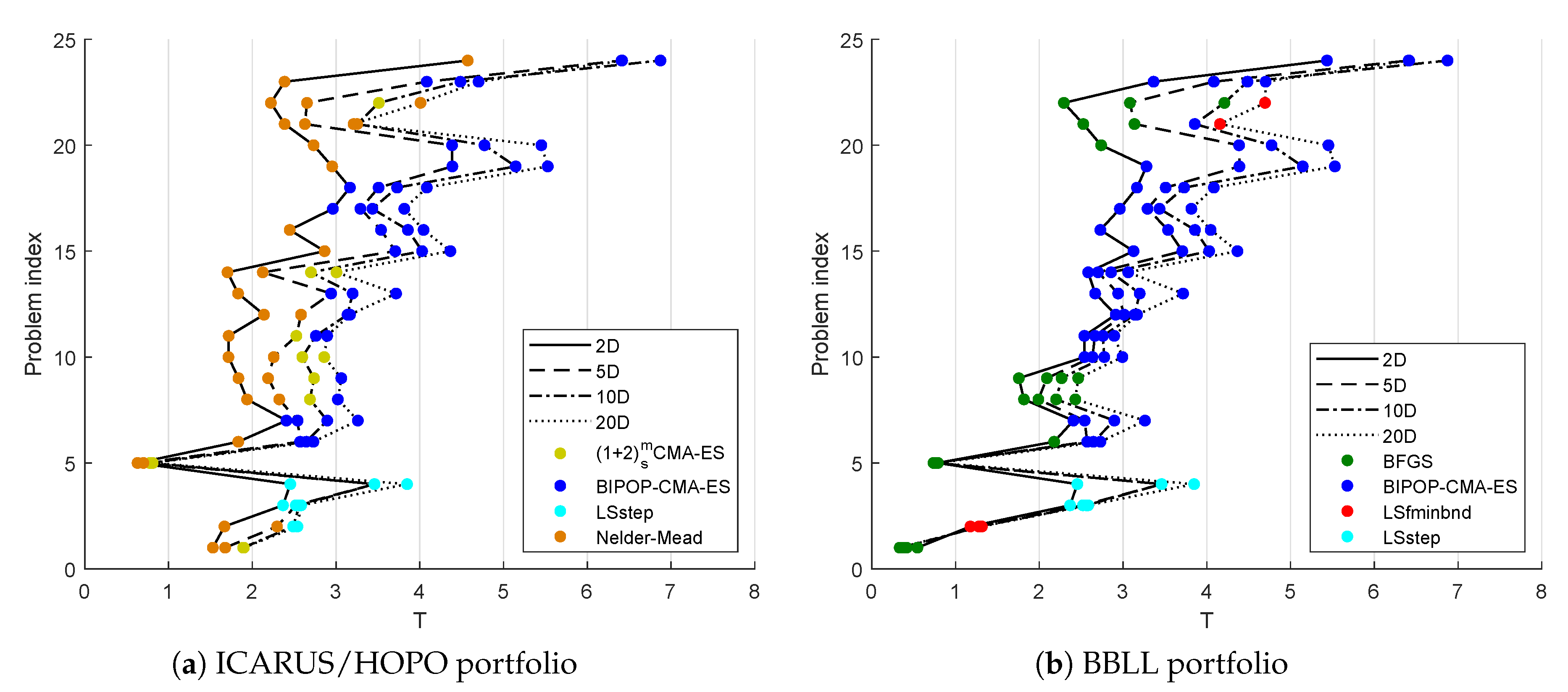
Figure 6.
Performance of the methods from Table 3 in terms of against . Figure (a) illustrates the performance of the individual algorithms, Figure (b) of the oracles and random selectors, Figure (c) of the selectors during HOIO, and Figure (d) of the selectors during HOPO. For the latter two figures, solid lines represent oracles using , while dashed lines represent oracles using . The shaded region indicates the theoretical area of performance, with the upper bound representing the ICARUS oracle and the lower bound random selection.

Table 1.
Summary of the ELA features employed in this paper. Each one of them was scaled using the listed approach.
Table 1.
Summary of the ELA features employed in this paper. Each one of them was scaled using the listed approach.
| Method | Feature | Description | Scaling |
|---|---|---|---|
| D | Dimensionality of the problem | ||
| Surrogate models | Adjusted coefficient of determination of a linear regression model including variable interactions | Unit scaling | |
| Adjusted coefficient of determination of a purely quadratic regression model | Unit scaling | ||
| Ratio between the minimum and the maximum absolute values of the quadratic term coefficients in the purely quadratic model | Unit scaling | ||
| Significance | Significance of D-th order | z-score, tanh | |
| Significance of first order | z-score, tanh | ||
| Cost distribution | Skewness of the cost distribution | z-score, tanh | |
| Kurtosis of the cost distribution | , z-score | ||
| Entropy of the cost distribution | , z-score |
Table 2.
Summary of the algorithms employed in this paper, which were selected using ICARUS [41] and the publicly available results from the BBOB sessions at the 2009 and 2010 GECCO Conferences. Algorithm names are as used for the dataset descriptions available at http://coco.gforge.inria.fr/doku.php?id=algorithms.
| Algorithm | Description | Reference |
|---|---|---|
| CMA-ES | A simple CMA-ES variant, with one parent and two offspring, sequential selection, mirroring and random restarts. All other parameters are set to the defaults. | [42] |
| BFGS | The MATLAB implementation (fminunc) of this quasi-Newton method, which is randomly restarted whenever a numerical error occurs. The Hessian matrix is iteratively approximated using forward finite differences, with a step size equal to the square root of the machine precision. Other than the default parameters, the function and step tolerances were set to and 0, respectively. | [43] |
| BIPOP-CMA-ES | A multistart CMA-ES variant with equal budgets for two interlaced restart strategies. After completing a first run with a population of size , the first strategy doubles the population size; while the second one keeps a small population given by , where is the latest population size from the first strategy, , and is an independent uniformly distributed random number. Therefore, . All other parameters are at default values. | [44] |
| LSfminbnd | The MATLAB implementation (fminbnd) of this axis parallel line search method, which is based on the golden section search and parabolic interpolation. It can identify the optimum of quadratic functions in a few steps. On the other hand, it is a local search technique; it can miss the global optimum (of the 1D function). | [45] |
| LSstep | An axis parallel line search method effective only on separable functions. To find a new solution, it optimizes over each variable independently, keeping every other variable fixed. The STEP version of this method uses interval division, i.e., it starts from an interval corresponding to the upper and lower bounds of a variable, which is divided by half at each iteration. The next sampled interval is based on its “difficulty,” i.e., by its belief of how hard it would be to improve the best-so-far solution by sampling from the respective interval. The measure of difficulty is the coefficient a from a quadratic function , which must go through the both interval boundary points. | [45] |
| Nelder–Mead | A version of the Nelder–Mead algorithm that uses random restarts, resizing and half-runs. In a resizing step, the current simplex is replaced by a “fat” simplex, which maintains the best vertex, but relocates the remaining ones such that they have the same average distance to the center of the simplex. Such steps are performed every 1000 algorithm iterations. In a half-run, the algorithm is stopped after interations, with only the most promising half-runs being allowed to continue. | [46] |
Table 3.
Performance of each algorithm and the selector, in terms of , 95% confidence interval of , and , which is the normalized performance score against random selection using the BBLL portfolio. In boldface are the lowest values for each performance measure over each validation method and n.
Table 3.
Performance of each algorithm and the selector, in terms of , 95% confidence interval of , and , which is the normalized performance score against random selection using the BBLL portfolio. In boldface are the lowest values for each performance measure over each validation method and n.
| CI | |||||||||
|---|---|---|---|---|---|---|---|---|---|
| CMA-ES | 2.852 | 66.7% | 1.511 | ||||||
| BFGS | 2.633 | 43.8% | 1.074 | ||||||
| BIPOP-CMA-ES | 3.397 | 95.8% | 1.823 | ||||||
| LSfminbnd | 3.092 | 27.1% | 0.566 | ||||||
| LSstep | 3.306 | 30.2% | 0.591 | ||||||
| Nelder–Mead | 2.765 | 59.4% | 1.388 | ||||||
| ICARUS | HOIO | 100 | 3.287 | 99.7% | 98.6% | 0.5% | 0.3% | 1.960 | |
| 178 | 3.341 | 99.6% | 98.9% | 0.3% | 0.3% | 1.926 | |||
| 316 | 3.417 | 99.7% | 98.9% | 0.4% | 0.2% | 1.885 | |||
| 562 | 3.509 | 99.8% | 99.1% | 0.3% | 0.2% | 1.837 | |||
| 1000 | 3.622 | 99.7% | 99.1% | 0.4% | 0.3% | 1.779 | |||
| ORACLE | 3.092 | 100.0% | 100.0% | 0.0% | 0.0% | 2.090 | |||
| RAND | 3.178 | 56.5% | 33.3% | 33.3% | 18.5% | 1.148 | |||
| HOPO | 100 | 3.269 | 93.6% | 60.6% | 4.2% | 2.0% | 1.851 | ||
| 178 | 3.293 | 92.5% | 55.9% | 4.3% | 0.7% | 1.814 | |||
| 316 | 3.371 | 93.8% | 61.1% | 4.7% | 1.9% | 1.798 | |||
| 562 | 3.510 | 95.4% | 60.9% | 5.9% | 1.3% | 1.756 | |||
| 1000 | 3.618 | 92.7% | 57.4% | 8.1% | 2.3% | 1.656 | |||
| ORACLE | 3.025 | 100.0% | 100.0% | 0.0% | 0.0% | 2.136 | |||
| RAND | 3.093 | 63.2% | 25.9% | 26.2% | 15.6% | 1.320 | |||
| BBLL | HOIO | 100 | 3.264 | 99.4% | 98.3% | 0.7% | 0.5% | 1.968 | |
| 178 | 3.321 | 99.5% | 98.8% | 0.6% | 0.4% | 1.936 | |||
| 316 | 3.401 | 99.5% | 98.8% | 0.5% | 0.4% | 1.891 | |||
| 562 | 3.495 | 99.7% | 99.1% | 0.5% | 0.3% | 1.843 | |||
| 1000 | 3.611 | 99.7% | 99.0% | 0.5% | 0.3% | 1.784 | |||
| HOPO | 100 | 3.228 | 87.7% | 59.7% | 10.2% | 6.7% | 1.755 | ||
| 178 | 3.310 | 90.0% | 60.2% | 9.6% | 4.7% | 1.757 | |||
| 316 | 3.353 | 88.5% | 59.8% | 9.6% | 5.7% | 1.707 | |||
| 562 | 3.435 | 88.5% | 58.6% | 8.2% | 5.4% | 1.665 | |||
| 1000 | 3.571 | 90.5% | 61.2% | 10.5% | 4.6% | 1.638 | |||
| ORACLE | 3.040 | 100.0% | 100.0% | 0.0% | 0.0% | 2.126 | |||
| RAND | 3.170 | 49.1% | 25.0% | 25.0% | 14.3% | 1.000 | |||
Table 4.
Average across all for a given problem at a given dimension during HOIO and HOPO validations, and average and for a given problem at a given dimension during HOPO validations. In boldface are the and less than 90%, and the higher than 10%.
Table 4.
Average across all for a given problem at a given dimension during HOIO and HOPO validations, and average and for a given problem at a given dimension during HOPO validations. In boldface are the and less than 90%, and the higher than 10%.
| HOIO | HOPO | |||||||
|---|---|---|---|---|---|---|---|---|
| 100.0% | 63.0% | 9.2% | 0.0% | 100.0% | 45.5% | 15.0% | 0.0% | |
| 100.0% | 69.8% | 13.7% | 0.0% | 100.0% | 55.0% | 19.5% | 0.0% | |
| 99.8% | 91.0% | 0.2% | 0.2% | 100.0% | 86.6% | 0.1% | 0.1% | |
| 98.0% | 89.1% | 1.3% | 1.0% | 95.2% | 82.2% | 2.4% | 2.2% | |
| 100.0% | 75.5% | 11.1% | 0.0% | 100.0% | 67.1% | 18.4% | 0.0% | |
| 98.7% | 88.8% | 0.1% | 0.1% | 98.4% | 86.9% | 0.2% | 0.2% | |
| 98.7% | 95.2% | 0.4% | 0.4% | 98.3% | 92.8% | 0.9% | 0.9% | |
| 98.6% | 74.1% | 1.4% | 1.4% | 93.0% | 59.6% | 7.0% | 7.0% | |
| 100.0% | 74.9% | 0.0% | 0.0% | 100.0% | 66.2% | 0.0% | 0.0% | |
| 99.5% | 83.6% | 0.4% | 0.4% | 99.5% | 76.2% | 0.4% | 0.4% | |
| 99.0% | 83.8% | 0.8% | 0.8% | 99.2% | 76.8% | 0.8% | 0.8% | |
| 94.0% | 81.7% | 2.2% | 0.0% | 91.6% | 76.4% | 1.8% | 0.0% | |
| 97.1% | 93.9% | 1.7% | 1.7% | 95.3% | 90.5% | 2.8% | 2.8% | |
| 95.7% | 79.9% | 4.3% | 4.3% | 93.5% | 70.7% | 6.5% | 6.5% | |
| 99.7% | 94.3% | 1.0% | 0.0% | 99.0% | 92.8% | 1.2% | 0.2% | |
| 99.1% | 94.9% | 0.6% | 0.6% | 99.2% | 95.4% | 0.5% | 0.5% | |
| 91.8% | 86.9% | 1.9% | 1.9% | 90.2% | 83.1% | 1.5% | 1.5% | |
| 97.3% | 92.7% | 2.5% | 2.5% | 97.0% | 91.1% | 2.8% | 2.8% | |
| 99.7% | 96.5% | 0.3% | 0.3% | 95.6% | 91.3% | 2.5% | 2.5% | |
| 90.0% | 81.9% | 3.2% | 0.0% | 85.5% | 74.5% | 3.2% | 0.0% | |
| 100.0% | 67.9% | 0.0% | 0.0% | 100.0% | 50.3% | 0.0% | 0.0% | |
| 100.0% | 75.7% | 0.0% | 0.0% | 100.0% | 67.8% | 0.0% | 0.0% | |
| 80.8% | 80.7% | 9.0% | 9.0% | 66.9% | 66.9% | 16.4% | 16.4% | |
| 76.2% | 71.8% | 9.1% | 9.1% | 71.5% | 68.0% | 13.9% | 13.9% | |
| 2 | 96.2% | 79.6% | 5.0% | 2.0% | 95.1% | 73.2% | 7.0% | 2.6% |
| 5 | 96.0% | 83.7% | 2.8% | 1.2% | 94.2% | 77.2% | 4.2% | 2.0% |
| 10 | 96.6% | 82.0% | 3.3% | 1.4% | 95.1% | 74.4% | 4.6% | 2.5% |
| 20 | 96.8% | 86.0% | 1.3% | 1.0% | 93.8% | 77.4% | 3.8% | 2.7% |
Table 5.
Bootstrapped 95% CI of . The sub-index represents the bias of the estimation. In boldface are those intervals whose range is the smallest for a given validation, and the lowest bias.
Table 5.
Bootstrapped 95% CI of . The sub-index represents the bias of the estimation. In boldface are those intervals whose range is the smallest for a given validation, and the lowest bias.
| ICARUS | HOIO | 100 | |||||
| 178 | |||||||
| 316 | |||||||
| 562 | |||||||
| 1000 | |||||||
| HOPO | 100 | ||||||
| 178 | |||||||
| 316 | |||||||
| 562 | |||||||
| 1000 | |||||||
| BBLL | HOIO | 100 | |||||
| 178 | |||||||
| 316 | |||||||
| 562 | |||||||
| 1000 | |||||||
| HOPO | 100 | ||||||
| 178 | |||||||
| 316 | |||||||
| 562 | |||||||
| 1000 |
Publisher’s Note: MDPI stays neutral with regard to jurisdictional claims in published maps and institutional affiliations. |
© 2021 by the authors. Licensee MDPI, Basel, Switzerland. This article is an open access article distributed under the terms and conditions of the Creative Commons Attribution (CC BY) license (http://creativecommons.org/licenses/by/4.0/).
Share and Cite
MDPI and ACS Style
Muñoz, M.A.; Kirley, M. Sampling Effects on Algorithm Selection for Continuous Black-Box Optimization. Algorithms 2021, 14, 19. https://0-doi-org.brum.beds.ac.uk/10.3390/a14010019
AMA Style
Muñoz MA, Kirley M. Sampling Effects on Algorithm Selection for Continuous Black-Box Optimization. Algorithms. 2021; 14(1):19. https://0-doi-org.brum.beds.ac.uk/10.3390/a14010019
Chicago/Turabian StyleMuñoz, Mario Andrés, and Michael Kirley. 2021. "Sampling Effects on Algorithm Selection for Continuous Black-Box Optimization" Algorithms 14, no. 1: 19. https://0-doi-org.brum.beds.ac.uk/10.3390/a14010019
Note that from the first issue of 2016, this journal uses article numbers instead of page numbers. See further details here.